Optimal Investment Strategy for DC Pension Plan with Deposit Loan Spread under the CEV Model

Abstract

This paper is devoted to determining an optimal investment strategy for a defined-contribution (DC) pension plan with deposit loan spread under the constant elasticity of variance (CEV) model. As far as we know, few studies in the literature have taken loans into account when using the CEV model in financial market contexts. The contribution of this paper is to study the impact of deposit loan spread on DC pension investment strategy. By considering a risk-free asset, a risky asset driven by CEV model, and a loan in the financial market, we first set up the dynamic equation and the asset market model, which are instrumental in achieving the expected utility of ultimate wealth at retirement. Second, the corresponding Hamilton–Jacobi–Bellman (HJB) equation is derived by means of the dynamic programming principle. The explicit expression for the optimal investment strategy is obtained using the Legendre transform method. Finally, different parameters are selected to simulate the explicit solution, and the financial interpretation of the optimal investment strategy is provided. We find that the deposit loan spread has a great impact on the investment strategy of DC pension plans.

1. Introduction

With the development of the global economy and society, pension planning is becoming more important for the life of the elderly. In addition, the aging of the population is accelerating rapidly, and pension planning has become a focus. The enterprise annuity is divided into two basic modes: defined benefit (DB) plans and the defined contribution (DC) plans. In DC pension plans, the longevity and financial risks are transferred from the sponsor to the member; thus, DC pension plans play a role in social security which cannot be ignored. Hence, asset allocation strategy is crucial to the distribution and deployment of DC pension funds.

In recent years, many scholars have focused on the optimal investment performance. Markowitz and Harry [1] put forward the optimal portfolio problem for the first time, and provided a theoretical proof. Boulier et al. [2] studied the asset allocation problem of DC-type enterprise funds where the interest rate obeys the the framework of Vasicek, and obtained the analytical solution through the use of the Martingale method. Haberman and Vigna [3] obtained a formula for the the optimal investment allocation in a DC pension scheme whose fund is invested in n assets. Gerrard et al. [4] concentrated on the income drawdown option using the stochastic optimal control technology to find optimal investment strategies after retirement. Baev and Bondarev [5] introduced O-U process instead of GBM. In [6,7], the investment strategy of a DC scheme was obtained through simulations using American and British data. Gao [8] examined the complete financial market with stochastic evolution of interest rate, and used Legendre transform to solve the optimal asset allocation strategy of a DC-type enterprise fund. In [9,10,11], the authors studied the optimal investment strategy for a DC plan in a mean-variance framework. Teng et al. [12] used an interest rate which was subject to the O–U process. Guan and Liang [13] studied the optimal allocation of a DC pension with a random interest rate and random fluctuation framework in which the interest rate obeyed an affine interest rate structure. Sun et al. [14] proposed the expected investment goal based on deficit and surplus. Bian et al. [15] and Chen et al. [16] investigated the DC pension fund investment problem under a Markovian regime-switching market consisting of one risk-free asset and multiple risky assets. Optimal investment with transaction cost over an infinite horizon was developed by Blake and Sass [17]. The dual control technique was employed to investigate the investment problem constrained by short selling in [18]. Dong and Zheng [19] attempted to apply S-shaped utility. Based on game theory and with the help of the filtering method and stochastic control theory, Wang et al. [20] obtained the equilibrium investment scheme of the mean variance criterion and the corresponding equilibrium value expression.

Several scholars have studied the DC pension problem under the random volatility model. In [21], the CRRA utility function was introduced to deal with the investment scheme in a random interest rate and volatility model. The optimal allocation scheme with stochastic interest rate and stochastic volatility was characterised by Wang et al. [22]. In Zhang et al. [23], a mean variance criterion under the Cox-Ingersoll-Ross (CIR) and stochastic volatility model was adopted. Other scholars have studied the DC pension problem in the context of inflation. Inflation risk and the optimal DC pension was considered in [24,25]. In [26], the authors studied a mean variance portfolio selection problem with stochastic salary and inflation protection strategy for a DC pension plan. Tang et al. [27] made an on-the-spot investigation of two different situations, namely, a random interest rate and annuity inflation. In Guambe et al. [28], the authors further stated an investment problem that included inflation and mortality risks. Wang et al. [29] studied a case where inflation of index bonds and expected yields obeyed the mean regression model. The continuous diffusion process and jump diffusion process were used to describe the price process of inflation index bonds and stocks in [30], and a DC pension problem was studied. Other scholars have studied DC pensions under the jump diffusion model. For example, a jump diffusion model was demonstrated by [31,32].

Several scholars have extended geometric Brownian motion to the CEV Model. Jianwu et al. [33] obtained an explicit solution by applying the CEV model. Gu et al. [34] considered the optimal reinsurance and investment problem of Brownian motion with a risk pricing process, and assets were described by the constant elastic variance model. Zhang and Rong [35] further paid attention to the optimal allocation of a DC pension with a random wage under the CEV model. Li et al. [36] used the game theory method to obtain the value function corresponding to the CEV Model. The equivalent balance fee and maximum technology were applied based on the CEV model in [37]. Ma et al. [38] used the least-squares Monte Carlo method concerning the framework of CEV. He and Chen [39] were interested in the stochastic interest rate, and added an asymptotic expansion method to approximate the asymptotic solution subject to the extended CEV in He et al. [40]. The lie symmetry method and group theory analysis received attention in Yong et al. [41], which used the CEV model.

Most of the above literature involves the CIR model, Vasicek model, variance model, or CEV model; however, few of them take loans based on the CEV model in financial markets into account. As is known, it is more accurate to adopt the CEV model, as it reflects the fluctuations in asset prices. What is more, with the upgrading and adjustment of China’s industry, capital driven by economic development is expected to become the main economic thrust; that is to say, the era of capital economy has arrived, and loan financing is now the normal state. In real life, the loan interest rate is higher than the deposit interest rate, and this difference has a noticeable impact on the investment of DC pensions. Therefore, this paper is devoted to studying a DC pension plan with deposit and loan spread under the CEV model. The goal is to maximize the expectation of the terminal wealth under the utility framework before retirement. By adopting the theory of stochastic control, the nonlinear HJB equation was achieved, in which it is hard to solve closed-form expressions. Then, we introduce the Legendre transform and separation of variables. In this case, nonlinear partial differential equations (NPDE) are transformed into linear partial differential equations. Finally, we derive the explicit expressions of the DC pension and provide the related financial explanation.

The rest of this paper is laid out as follows. Section 2 characterizes the assumptions of the model. Section 3 presents the definition of the value function and derives the corresponding HJB equation using the dynamic programming principle. Section 4 completes the closed-form solutions for the stochastic dynamic programming problem with Legendre transform and the CRRA utility function. Section 5 presents a numerical simulation analysis. FInally, Section 6 provides a summary and concludes the paper.

2. Model Hypothesis

We list the following assumptions for our model.

Consider a financial market which ignores transaction fees. We use a finite time horizon and continuous time model. $\{W_t,t\ge 0\}$ represents the standard Brownian motion for a complete probability space $(\mathsf{\Omega },\mathcal{F},\mathbb{P})$, where $\mathbb{P}$ is the real-word probability and $\mathcal{F}=\left\{{\mathcal{F}}_t\right\}$ denotes the $\mathbb{P}$-augmentation of the natural filtration produced by ${\left\{W_t\right\}}_{t\in [0,T]}$. We assume that all of the stochastic processes introduced below are well defined on the probability space $(\mathsf{\Omega },\mathcal{F},\mathbb{P})$ and adapted to the filtration ${\left\{{\mathcal{F}}_t\right\}}_{t\in [0,T]}$.

Suppose that the financial market involves three tradeable assets: a bank account, a stock, and a loan. We denote the price of the bank account at time t by $B_t$, such that

$$d{B}_t=r{B}_{t}dt,$$

(1)

where $r>0$ is a constant rate of interest.

By comparison with GBM, the CEV model is closer to the change in the stock price. Here, we use $S_t$ to express the price of the stock at time t, which is described by the CEV model as follows:

$$d{S}_t=\mu S_{t}dt+k{S}_t^{\beta +1}d{W}_t,$$

(2)

where $\mu$ ($\mu >r$) is the expected instantaneous rate of return of the stock, k and $\beta$ are constant parameters, $\beta$ satisfies the general condition $\beta <0$, and $k{S}_t^{\beta }$ is the instantaneous volatility.

Let R denote the lending rate, where $0<r<R<\mu$, where $V_t$ is the pension wealth at time t and $L_t$, $X_t$, and $Y_t$ are the total amount of money of the loan, the risk-free asset, and the risky asset, respectively, at time t.

Definition 1.

(Admissible strategy) An investment loan is admissible if it meets the following requirements:

(1) $\{L_t,X_t,Y_t\}$ is ${\mathcal{F}}_t$-measurable on a complete probability space

(2) ${\int }_0^T{L}_t^{2}dt<+\infty$, ${\int }_0^T{X}_t^{2}dt<+\infty$, ${\int }_0^T{Y}_t^{2}dt<+\infty$, a.s. $T<\infty$

(3) For rational investors, with interest rates higher than the deposit rate it is impossible to choose between deposits and loans; that is, $L_t{X}_t=0$, with $L_t\ge 0$, $X_t\ge 0$ and $t\in [0,T]$. The strategies $\{L_t,X_t,Y_t\}$ take values in a control set Π.

Moreover, define the retirement moment and the contribution rate of the enterprise annuity for T and c separately, where T and c are constants. Until retirement T, $c{L}_t$ is supplied to the pension fund for each period. In order to simplify the model, the total salary is set as one dollar, and only one insured person is studied.

3. Model Formulation

3.1. Wealth Process

Let $V_t=X_t+Y_t-L_t+ct$ denote the pension wealth at time $t\in [0,T]$. The dynamics of wealth have the following form:

$$\begin{array}{c}\hfill d{V}_t=\frac{X_t}{B_t}d{B}_t+\frac{Y_t}{S_t}d{S}_t-R{L}_{t}dt+cdt.\end{array}$$

(3)

Based on (1) and (2), we can rewrite (3) as

$$\begin{array}{c}\hfill d{V}_t=[r{V}_t+(\mu -r)Y_t+(r-R)L_t-rct+c]dt+k{S}^{\beta }{Y}_{t}d{W}_t.\end{array}$$

(4)

3.2. The HJB Equation

Next, the goal is to maximize the expected discounted utility and ultimate wealth over a limited retirement period, i.e., to seek the optimum investment project.

Applying the stochastic control theory, we define the value function as

$$H(t,s,v)=\underset{\{L,X,Y\}\in \mathsf{\Pi }}{sup}E\left[U\left(V_T\right)|S_t=s,V_t=v\right],0<t<T,$$

where $U(·)$ is an increasing concave utility function and satisfies the conditions $U^{\prime }(+\infty )<0$ and $U^{\prime }\left(0\right)<+\infty$.

As described in [42] and per It$\widehat{o}$’s formula and dynamic programming principle, we have

$$\begin{array}{cc}\hfill \underset{\{L,X,Y\}\in \mathsf{\Pi }}{sup}\{H_t+& [rv+(\mu -r)Y+(r-R)L-rct+c]H_v+\mu s{H}_s\hfill \\ \hfill +& \frac{1}{2}{k}^2{s}^{2\beta }{Y}^2{H}_{vv}+\frac{1}{2}{k}^2{s}^{2\beta +2}{H}_{ss}+k^2{s}^{2\beta +1}Y{H}_{vs}\}=0,\hfill \end{array}$$

(5)

and its accompanying a terminal condition, $H(T,s,v)=U\left(v\right)$.

According to $v=V_t=B_t+Y_t-L_t+ct$ and $0<r<R<\mu$, if $v>Y_t+ct$, the investor rejects the loan, while if $v\le Y_t+ct$, the investor chooses the loan and the total amount will not exceed $Y_t+ct-v$, that is, $L_t^{*}=Y_t+ct-v=max\{0,Y_t+ct-v\}$.

From the above setting, the following two situations are discussed:

(1) In the case where $v>Y_t+ct$, by substituting $L_t^{*}=0$ into (5) the corresponding HJB equation can be rewritten as

$$\left\{\begin{array}{cc}\hfill & \underset{Y\in \mathsf{\Pi }}{sup}\{H_t+[rv+(\mu -r)Y-rct+c]H_v+\mu s{H}_s\hfill \\ \hfill & +\frac{1}{2}{k}^2{s}^{2\beta }{Y}^2{H}_{vv}+\frac{1}{2}{k}^2{s}^{2\beta +2}{H}_{ss}+k^2{s}^{2\beta +1}Y{H}_{vs}\}=0\hfill \\ \hfill & H(T,s,v)=U\left(v\right).\hfill \end{array}\right.$$

(6)

(2) In the case where $v\le Y_t+ct$, by substituting $L_t^{*}=Y_t+ct-v$ into (5) the corresponding HJB equation can be rewritten as

$$\left\{\begin{array}{cc}\hfill & \underset{Y\in \mathsf{\Pi }}{sup}\{H_t+[Rv+(\mu -R)Y-Rct+c]H_v+\mu s{H}_s\hfill \\ \hfill & +\frac{1}{2}{k}^2{s}^{2\beta }{Y}^2{H}_{vv}+\frac{1}{2}{k}^2{s}^{2\beta +2}{H}_{ss}+k^2{s}^{2\beta +1}Y{H}_{vs}\}=0\hfill \\ \hfill & H(T,s,v)=U\left(v\right).\hfill \end{array}\right.$$

(7)

If we take the derivative of (6) with respect to Y, we have

$$\begin{array}{cc}\hfill Y_{1t}^{*}=& -\frac{\mu -r}{k^2{s}^{2\beta }}\frac{H_v}{H_{vv}}-s\frac{H_{vs}}{H_{vv}}.\hfill \end{array}$$

(8)

Similarly, we can obtain the efficient investment strategy of problem (7) as follows:

$$\begin{array}{cc}\hfill Y_{2t}^{*}=& -\frac{\mu -R}{k^2{s}^{2\beta }}\frac{H_v}{H_{vv}}-s\frac{H_{vs}}{H_{vv}}.\hfill \end{array}$$

(9)

Using $Y_{1t}^{*}$ and $Y_{2t}^{*}$ in (6) and (7), we respectively derive

$$\begin{array}{cc}\hfill H_t+& \mu s{H}_s+\frac{1}{2}{k}^2{s}^{2\beta +2}{H}_{ss}+(rv-rct+c)H_v-\frac{{(\mu -r)}^2}{2k^2{s}^{2\beta }}\frac{H_v^2}{H_{vv}}\hfill \\ \hfill -& \frac{1}{2}{k}^2{s}^{2\beta +2}\frac{H_{vs}^2}{H_{vv}}-s(\mu -r)\frac{H_v{H}_{vs}}{H_{vv}}=0,\hfill \end{array}$$

(10)

and

$$\begin{array}{cc}\hfill H_t+& \mu s{H}_s+\frac{1}{2}{k}^2{s}^{2\beta +2}{H}_{ss}+(Rv-Rct+c)H_v-\frac{{(\mu -R)}^2}{2k^2{s}^{2\beta }}\frac{H_v^2}{H_{vv}}\hfill \\ \hfill -& \frac{1}{2}{k}^2{s}^{2\beta +2}\frac{H_{vs}^2}{H_{vv}}-s(\mu -R)\frac{H_v{H}_{vs}}{H_{vv}}=0.\hfill \end{array}$$

(11)

Obviously, the stochastic control problem is transformed into an NPDE. Next, we alternate the NPDE into the linear PDE based on dual transformation.

4. Verification Theorem

In this section, the verification theorem is established through the standard method used by Halil Mete Soner in [42].

Theorem 1.

Suppose $H\in C^{1,2,2}\left(Q\right)\cap C\left(\overline{Q}\right)$ is a solution to Equation (6) (Equation (7)) where $Q:=(0,T)\times (0,\infty )\times (-\infty ,\infty )$; then:

• $H(t,s,v)\ge G(t,s,v;Y.)$ for any initial value $(t,s,v)\in Q$ and control process $Y.$, where $G(t,s,v;Y.)=E\left[U\left(V_T\right)\right|S_t=s,V_t=v]$
• If, for any initial value $(t,s,v)\in Q$, there exists $Y^{*}.\in \mathsf{\Pi }$ satisfying

  $$Y^{*}.\in argmax\left\{{\mathbb{B}}^{Y_{.}^{*},r}H\right\}\left(argmax\left\{{\mathbb{B}}^{Y_{.}^{*},R}H\right\}\right),$$
  then $H(t,s,v)=G(t,s,v;Y^{*}.)$. Here, the operator ${\mathbb{B}}^{Y,\lambda }$ is defined as follows:

  $${\mathbb{B}}^{Y,\lambda }H=[\lambda v+(\mu -\lambda )Y-\lambda ct+c]H_v+\mu s{H}_s+\frac{1}{2}{k}^2{s}^{2\beta }{Y}^2{H}_{vv}$$

  $$+\frac{1}{2}{k}^2{s}^{2\beta +2}{H}_{ss}+k^2{s}^{2\beta +1}Y{H}_{vs}.$$

Proof. 

We only prove that the theorem is valid when H is a solution to Equation (6), and we can prove it in a similar way when H is a solution to Equation (7).

(1) Using It$\widehat{o}$’s formula, we obtain

$$EH(T,s_T,v_T)=H(t,s,v)+E{\int }_t^T\left[\frac{\partial }{\partial \tau }H(\tau ,s_{\tau },v_{\tau })+{\mathbb{B}}^{Y_{\tau },r}H(\tau ,s_{\tau },v_{\tau })\right]d\tau .$$

Because H is a solution to Equation (6), we have

$$\frac{\partial }{\partial \tau }H(\tau ,s_{\tau },v_{\tau })+{\mathbb{B}}^{{\pi }_{\tau },r}H(\tau ,s_{\tau },v_{\tau })\le 0.$$

Therefore,

$$H(t,s,v)\ge EH(T,s_T,v_T).$$

Due to the terminal condition, we have

$$H(t,s,v)\ge G(t,s,v;Y.);$$

(2) Similarly,

$$EH(T,s_T,v_T^{*})=H(t,s,v)+E{\int }_t^T\left[\frac{\partial }{\partial \tau }H(\tau ,s_{\tau },v_{\tau }^{*})+{\mathbb{B}}^{{\pi }_{\tau }^{*},r}H(\tau ,s_{\tau },v_{\tau }^{*})\right]d\tau .$$

Because H is a solution to Equation (6), we have

$$\frac{\partial }{\partial \tau }H(\tau ,s_{\tau },v_{\tau }^{*})+{\mathbb{B}}^{{\pi }_{\tau }^{*},r}H(\tau ,s_{\tau },v_{\tau }^{*})=0.$$

Thus,

$$EH(T,s_T,v_T^{*})=H(t,s,v).$$

Due to the terminal condition, we have

$$H(t,s,v)=G(t,s,v;Y^{*}.).$$

□

5. Model Solution

5.1. Legendre Transform

Definition 2

(see [43]). Let f: $R^n\to R$ be a convex function; then, for $z>0$, the Legendre transform can be defined as follows:

$$\widehat{L}\left(z\right)=\underset{v}{max}\left\{f\left(v\right)-zv\right\},$$

where the function $\widehat{L}\left(z\right)$ is called the Legendre dual of the function $f\left(v\right)$.

A specific definition is proposed by

$$\widehat{H}(t,s,z)=\underset{v>0}{sup}\{H(t,s,v)-zv|0<t<T\},$$

where $z>0$ denotes the dual variable of v.

The value of v with this optimum is denoted by $g(t,s,z)$, such that

$$g(t,s,z)=\underset{v>0}{inf}\left\{v\right|H(t,s,v)\ge zv+\widehat{H}(t,s,v)\},0<t<T.$$

From the above equation, we can obtain

$$\widehat{H}(t,s,z)=H(t,s,g)-zg,$$

(12)

where $g(t,s,z)=v$ and $H_v=z$.

The function $\widehat{H}$ is related to g by

$$g=-{\widehat{H}}_z.$$

(13)

By differentiating (12), we achieve

$$H_v=z,H_t={\widehat{H}}_t,H_s={\widehat{H}}_s,H_{vv}=-\frac{1}{{\widehat{H}}_{zz}},H_{ss}={\widehat{H}}_{ss}-\frac{{\widehat{H}}_{sz}^2}{{\widehat{H}}_{zz}},H_{sv}=-\frac{\widehat{H}{}_{sz}}{{\widehat{H}}_{zz}}.$$

(14)

At the terminal time, T, we define

$$\begin{array}{cc}\hfill \widehat{U}\left(z\right)=& \underset{v>0}{sup}\{U\left(v\right)-zv\},\hfill \\ \hfill G\left(z\right)=& \underset{v>0}{inf}\{U\left(v\right)\ge zv+\widehat{U}\left(z\right)\}.\hfill \end{array}$$

(15)

In addition, there exists $G\left(z\right)={\left(U^{\prime }\right)}^{-1}\left(z\right)$.

Using (14) in (10), we derive

$$\begin{array}{cc}\hfill {\widehat{H}}_t+& \mu s{\widehat{H}}_s+\frac{1}{2}{k}^2{s}^{2\beta +2}{\widehat{H}}_{ss}+(rv-rct+c)z\hfill \\ \hfill +& \frac{{(\mu -r)}^2{z}^2{\widehat{H}}_{zz}}{2k^2{s}^{2\beta }}-s(\mu -r)z{\widehat{H}}_{sz}=0.\hfill \end{array}$$

(16)

Differentiating both sides of (16) with respect to z, we obtain

$$\begin{array}{cc}\hfill {\widehat{H}}_{tz}+& \mu s{\widehat{H}}_{sz}+\frac{1}{2}{k}^2{s}^{2\beta +2}{\widehat{H}}_{ssz}+(rv-rct+c)+rz{g}_z+\frac{{(\mu -r)}^{2}z{\widehat{H}}_{zz}}{k^2{s}^{2\beta }}\hfill \\ \hfill +& \frac{{(\mu -r)}^2{z}^2{\widehat{H}}_{zzz}}{2k^2{s}^{2\beta }}-s(\mu -r){\widehat{H}}_{sz}-s(\mu -r)z{\widehat{H}}_{szz}=0.\hfill \\ \hfill \end{array}$$

(17)

Due to (13), we have

$$\begin{array}{cc}\hfill v=g=& -{\widehat{H}}_z,{\widehat{H}}_{tz}=-g_t,{\widehat{H}}_{sz}=-g_s,{\widehat{H}}_{zz}=-g_z,\hfill \\ \hfill {\widehat{H}}_{ssz}=& -g_{ss},{\widehat{H}}_{szz}=-g_{sz},{\widehat{H}}_{zzz}=-g_{zz}.\hfill \end{array}$$

(18)

We recover (17) using (18), then obtain the following partial differential equation:

$$\begin{array}{cc}\hfill g_t+& \mu s{g}_s+\frac{1}{2}{k}^2{s}^{2\beta +2}{g}_{ss}-(rg-rct+c)-rz{g}_z+\frac{{(\mu -r)}^{2}z{g}_z}{k^2{s}^{2\beta }}\hfill \\ \hfill +& \frac{{(\mu -r)}^2{z}^2{g}_{zz}}{2k^2{s}^{2\beta }}-s(\mu -r)g_s-s(\mu -r)z{g}_{sz}=0.\hfill \end{array}$$

(19)

Through dual transformation, (10) has now been transformed into a linear PDE. Moreover, we obtain the optimal portfolio selection, $Y_{1t}^{*}$:

$$\begin{array}{c}\hfill Y_{1t}^{*}=-\frac{\mu -r}{k^2{s}^{2\beta }}z{g}_z+s{g}_s.\end{array}$$

(20)

5.2. The Solution under the Logarithmic Utility Function

Theorem 2.

If the price of the risk-free asset, the price of the risky asset, and the wealth process follow (1)–(3), respectively, the optimal portfolio of the enterprise annuity is

$$Y_t^{*}=\left\{\begin{array}{cc}\hfill & \frac{(\mu -R)[v-ct+cT{e}^{R(t-T)}]}{k^2{s}^{2\beta }},v\le ct+\frac{(\mu -R)[v-ct+cT{e}^{R(t-T)}]}{k^2{s}^{2\beta }}\hfill \\ \hfill & v-ct,\frac{(\mu -R)[v-ct+cT{e}^{R(t-T)}]}{k^2{s}^{2\beta }}+ct<v<\frac{(\mu -r)[v-ct+cT{e}^{r(t-T)}]}{k^2{s}^{2\beta }}+ct\hfill \\ \hfill & \frac{(\mu -r)[v-ct+cT{e}^{r(t-T)}]}{k^2{s}^{2\beta }}.v\ge ct+\frac{(\mu -r)[v-ct+cT{e}^{r(t-T)}]}{k^2{s}^{2\beta }}\hfill \end{array}\right.$$

(21)

Proof. 

In light of the logarithmic utility function, the following definition is provided:

$$U\left(v\right)=lnv.x>0.$$

Depending on the form of the logarithmic utility function, we have

$$g(T,s,z)=\frac{1}{z}.$$

In response to (19), we construct its corresponding solution:

$$g(t,s,z)=\frac{1}{z}f\left(s_t\right)+\phi \left(t\right).$$

(22)

In the meantime, we quote the boundary conditions by $f\left(s_T\right)=1$ and $\phi \left(T\right)=0$.

Taking the partial derivative of (22), we have

$$\begin{array}{cc}\hfill g_t=& {\phi }_t,g_s=\frac{1}{z}{f}_s,g_z=-\frac{1}{z^2}f,\hfill \\ \hfill g_{ss}=& \frac{1}{z}{f}_{ss},g_{sz}=-\frac{1}{z^2}{f}_s,g_{zz}=\frac{2}{z^3}f.\hfill \end{array}$$

(23)

Substituting (23) back into (19), we obtain

$${\phi }_t+\mu s\frac{1}{z}{f}_s+\frac{k^2{s}^{2\beta +2}}{2}\frac{1}{z}{f}_{ss}+rct-c-r\phi =0.$$

(24)

By observation, (24) can be decomposed into two equations, which eliminates the dependence on s. Furthermore, as the boundary conditions are $f\left(s_T\right)=1$ and $\phi \left(T\right)=0$, we have

$$\left\{\begin{array}{cc}\hfill & \mu s{f}_s+\frac{k^2{s}^{2\beta +2}}{2}{f}_{ss}=0,\hfill \\ \hfill & f\left(s_T\right)=1.\hfill \end{array}\right.$$

(25)

and

$$\left\{\begin{array}{cc}\hfill & {\phi }_t-r\phi +rct-c=0,\hfill \\ \hfill & \phi \left(T\right)=0.\hfill \end{array}\right.$$

(26)

By solving these ordinary differential equations, we derive the solution to (25)

$$f\left(s_t\right)=1.$$

The corresponding solution of (26) is provided by

$$\phi \left(t\right)=ct-cT{e}^{r(t-T)}.$$

Consequently,

$$g=\frac{1}{z}+ct-cT{e}^{r(t-T)}.$$

(27)

Due to $g(t,s,z)=v$, we derive

$$\frac{1}{z}=v-ct+cT{e}^{r(t-T)}.$$

(28)

Finally, the optimal strategy $Y_{1t}^{*}$ can be rewritten as

$$\begin{array}{cc}\hfill Y_{1t}^{*}=& -\frac{\mu -r}{k^2{s}^{2\beta }}z{g}_z+s{g}_s\hfill \\ \hfill =& \frac{\mu -r}{k^2{s}^{2\beta }z}\hfill \\ \hfill =& \frac{(\mu -r)[v-ct+cT{e}^{r(t-T)}]}{k^2{s}^{2\beta }}.\hfill \end{array}$$

(29)

From the equivalence of r and R, we can obtain another optimal investment strategy, $Y_{2t}^{*}$:

$$\begin{array}{c}\hfill Y_{2t}^{*}=\frac{(\mu -R)[v-ct+cT{e}^{R(t-T)}]}{k^2{s}^{2\beta }}.\end{array}$$

(30)

The above results are discussed as follows.

(1) If ${\displaystyle v\ge \frac{(\mu -r)[v-ct+cT{e}^{r(t-T)}]}{k^2{s}^{2\beta }}+ct}$, then

$$\begin{array}{c}\hfill Y_{1t}^{*}=\frac{(\mu -r)[v-ct+cT{e}^{r(t-T)}]}{k^2{s}^{2\beta }};\end{array}$$

(2) If ${\displaystyle v\le \frac{(\mu -R)[v-ct+cT{e}^{R(t-T)}]}{k^2{s}^{2\beta }}+ct}$, then

$$\begin{array}{c}\hfill {\displaystyle Y_{2t}^{*}=\frac{(\mu -R)[v-ct+cT{e}^{R(t-T)}]}{k^2{s}^{2\beta }};}\end{array}$$

(3) If ${\displaystyle \frac{(\mu -r)[v-ct+cT{e}^{r(t-T)}]}{k^2{s}^{2\beta }}+ct>v>\frac{(\mu -R)[v-ct+cT{e}^{R(t-T)}]}{k^2{s}^{2\beta }}+ct}$, we proceed with two cases.

(i) When ${\displaystyle Y_t+ct\in [\frac{(\mu -R)[v-ct+cT{e}^{R(t-T)}]}{k^2{s}^{2\beta }}+ct,v]}$, as $L_t^{*}=Y_t+ct-v=max\{0,Y_t+ct-v\}$, then $L_t^{*}=0$. This means that the investor refuses to lend in this case. Let the left bracket of (6) be ${\varphi }_1\left(Y\right)$; because ${\varphi }_1\left(Y\right)$ increases with respect to Y in ${\displaystyle [\frac{(\mu -R)[v-ct+cT{e}^{R(t-T)}]}{k^2{s}^{2\beta }},v-ct]}$, it is apparent that ${\varphi }_1\left(Y\right)$ attains its maximum at $Y_t^{*}=v-ct$.

(ii) When ${\displaystyle Y_t+ct\in [v,\frac{(\mu -r)[v-ct+cT{e}^{r(t-T)}]}{k^2{s}^{2\beta }}+ct]}$, because $L_t^{*}=Y_t+ct-v=max\{0,Y_t+ct-v\}$, we can see that $L_t^{*}=v-ct$. We denote the left bracket of (7) by ${\varphi }_2\left(Y\right)$. Considering that ${\varphi }_2\left(Y\right)$ decreases with respect to Y in the interval ${\displaystyle [v-ct,\frac{(\mu -r)[v-ct+cT{e}^{R(t-T)}]}{k^2{s}^{2\beta }}]}$, we can see that ${\varphi }_2\left(Y\right)$ reaches the maximum at $Y_t^{*}=v-ct$. Hence, in the interval ${\displaystyle [\frac{(\mu -R)[v-ct+cT{e}^{R(t-T)}]}{k^2{s}^{2\beta }},\frac{(\mu -r)[v-ct+cT{e}^{r(t-T)}]}{k^2{s}^{2\beta }}]}$, it is apparent that $Y^{*}\left(t\right)=v-ct$.

Finally, the optimal investment strategy $Y_t^{*}$ can be expressed as

$$Y_t^{*}=\left\{\begin{array}{cc}\hfill & \frac{(\mu -R)[v-ct+cT{e}^{R(t-T)}]}{k^2{s}^{2\beta }},v\le ct+\frac{(\mu -R)[v-ct+cT{e}^{R(t-T)}]}{k^2{s}^{2\beta }}\hfill \\ \hfill & v-ct,\frac{(\mu -R)[v-ct+cT{e}^{R(t-T)}]}{k^2{s}^{2\beta }}+ct<v<\frac{(\mu -r)[v-ct+cT{e}^{r(t-T)}]}{k^2{s}^{2\beta }}+ct\hfill \\ \hfill & \frac{(\mu -r)[v-ct+cT{e}^{r(t-T)}]}{k^2{s}^{2\beta }}.v\ge ct+\frac{(\mu -r)[v-ct+cT{e}^{r(t-T)}]}{k^2{s}^{2\beta }}\hfill \end{array}\right.$$

□

Theorem 3.

If the price of the risk-free asset, the price of the risky asset, and the wealth process follow (1)–(3), respectively, the expected maximum utility of the enterprise annuity for problems (10) and (11) is as follows:

(1) In the case of $v\ge Y_t+ct$,

$$H_1=ln(v-ct+cT{e}^{r(t-T)}).$$

(2) In the case of $v<Y_t+ct$,

$$H_2=ln(v-ct+cT{e}^{R(t-T)}).$$

Proof. 

We first prove the former case. Combining (27) with $-{\widehat{H}}_z(t,s,v)=g$, we have

$${\widehat{H}}_z=-\frac{1}{z}-ct+cT{e}^{r(t-T)}.$$

(31)

From (31), integrating yields

$$\widehat{H}=-lnz+-ctz+czT{e}^{r(t-T)}+m,$$

where m is a constant.

Taking into account $\widehat{H}=H-zg$ and the terminal condition $m=-1$, we obtain

$$H_1=ln(v-ct+cT{e}^{r(t-T)}).$$

By the same token, we derive

$$H_2=ln(v-ct+cT{e}^{R(t-T)}).$$

□

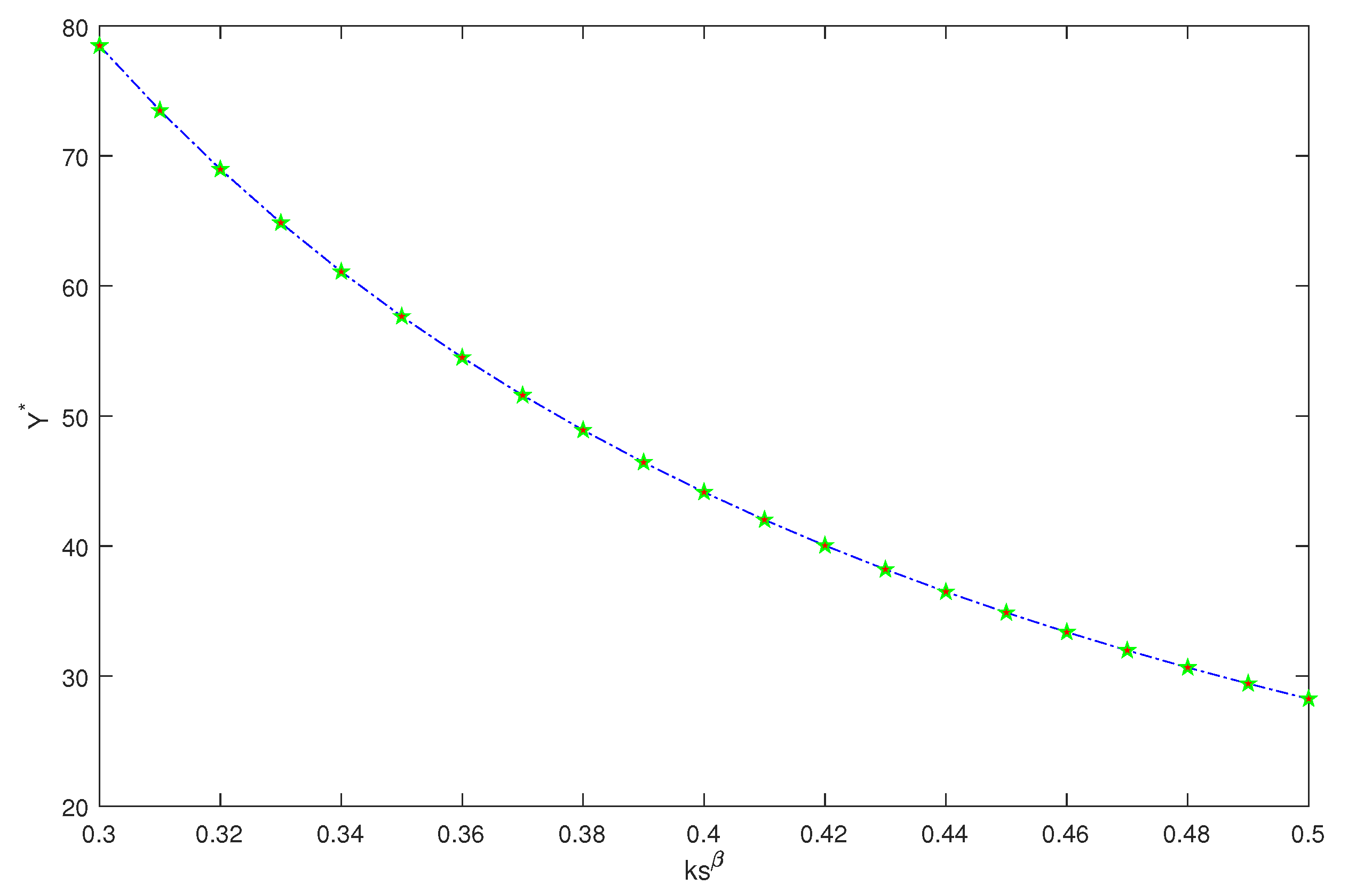
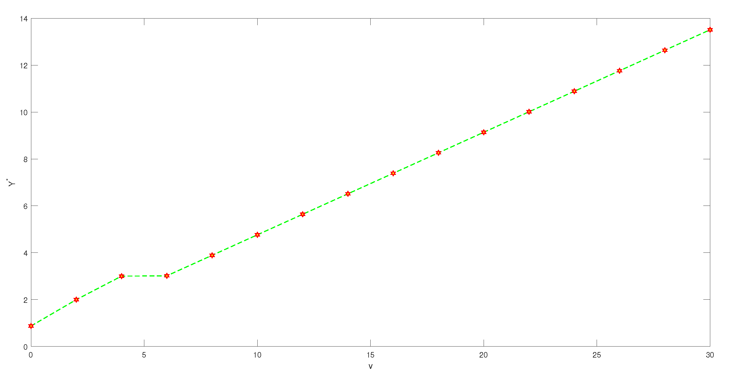
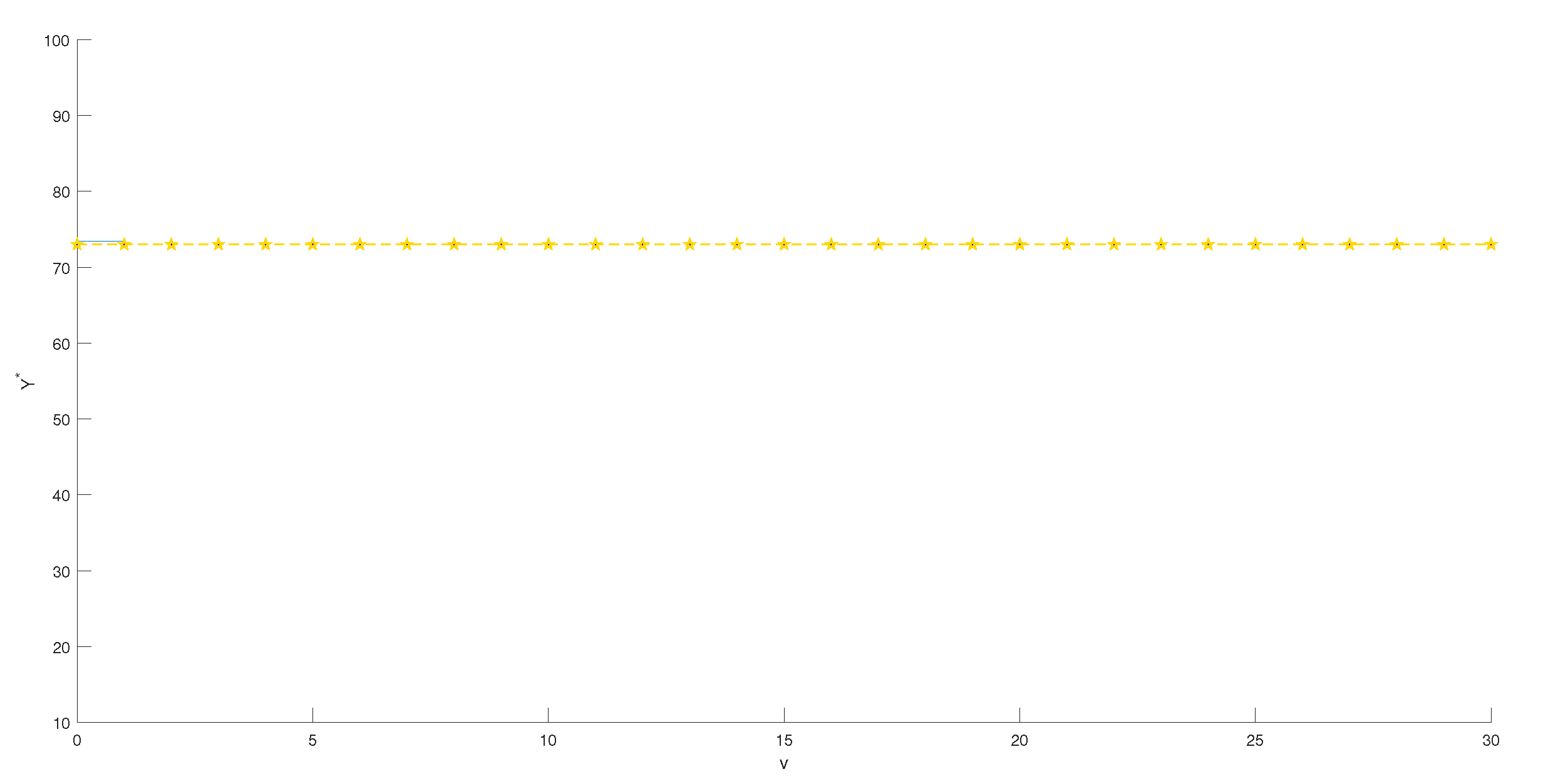
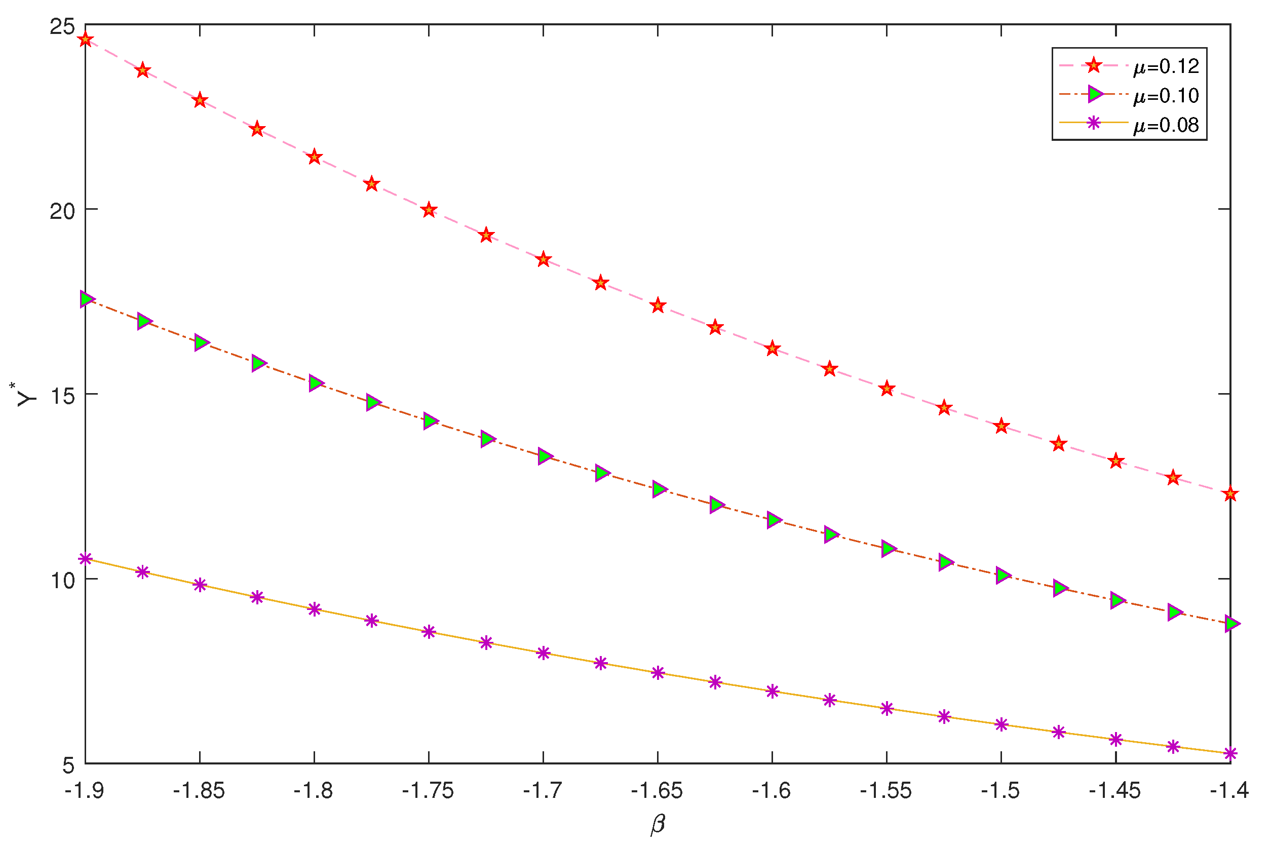
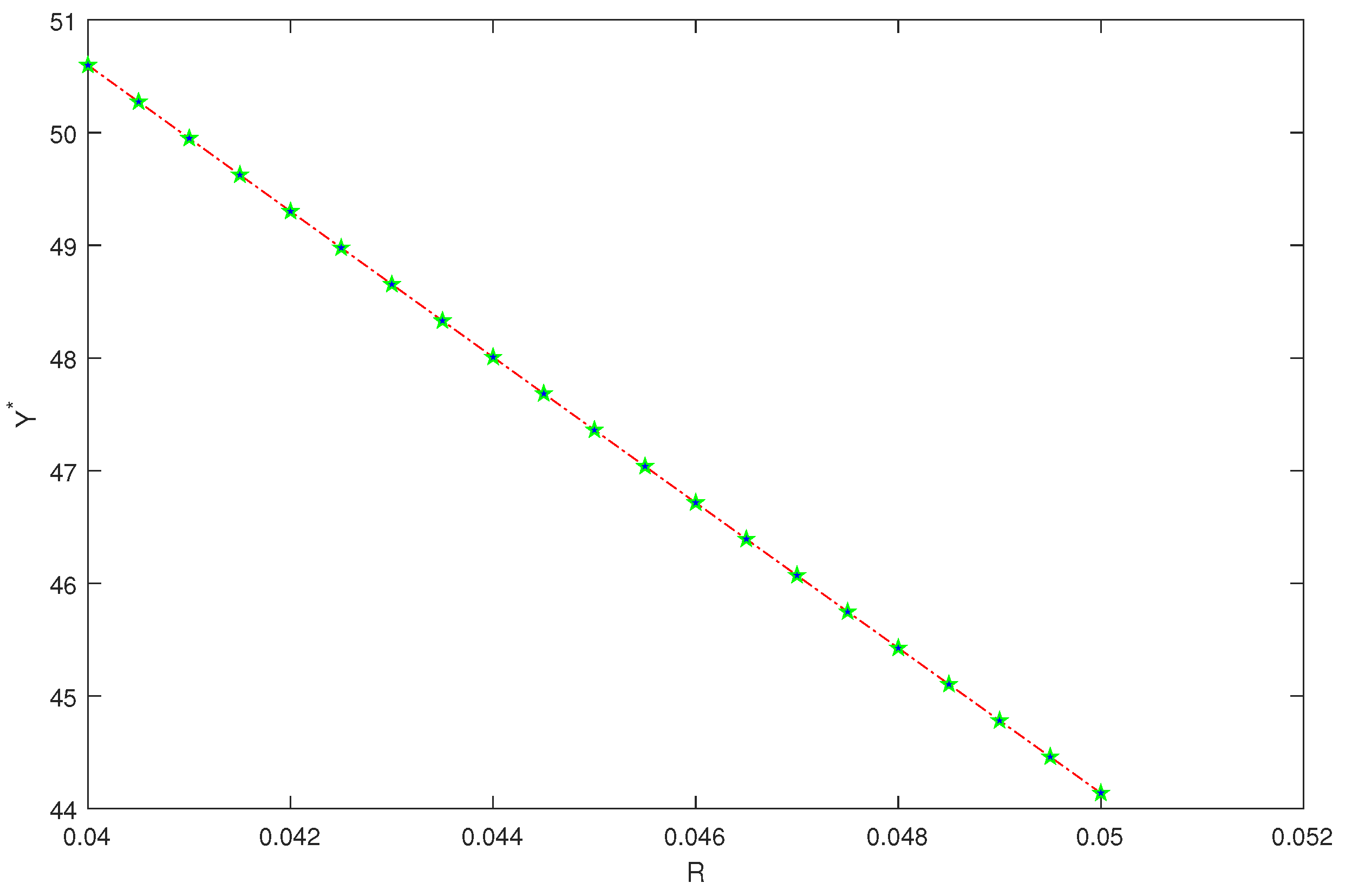
6. Numerical Analysis

Based on simulation results, we provide economic explanations for the above and discuss the behavioral features related to loss aversion and contribution rate. We take the initial time $t=5$, and assume the investor retires at $T=20$. In the financial market, the other parameters used are $r=0.03$, $R=0.05$, ${\sigma }_1=0.005$ and $c=0.2$.

In Figure 1 and Figure 2, the volatility, $k{S^{\beta }}_t$, in the optimal investment strategy $Y_t^{*}$ is taken into account. Assume that the wealth value is 5, 100 at time t, and the volatility $k{S^{\beta }}_t$ varies at $[0.05,0.25]$. If $v=5$, then $v\le ct+\frac{(\mu -R)[v-ct+cT{e}^{R(t-T)}]}{k^2{s}^{2\beta }}$. If $k{S^{\beta }}_t$ varies in the range $[0.3,0.5]$ and $v=100$, then $v\ge ct+\frac{(\mu -r)[v-ct+cT{e}^{r(t-T)}]}{k^2{s}^{2\beta }}$.

Figure 1 and Figure 2 demonstrate how $k{S^{\beta }}_t$ affects the optimal investment strategy $Y_t^{*}$ for investing in the risky asset. Evidently, the increase of $k{S^{\beta }}_t$ causes the reduction of $Y_t^{*}$, which signifies that investors provide fewer funds to the risky asset when the stock price fluctuation increases. From a financial perspective, this can be interpreted as the stock price fluctuation enhancing the uncertainty in the market. At the same time, the risky asset faces the possibility of depreciation. In response to this situation, investors do not dare to engage in radical adventure, and instead prefer conservative investments.

Figure 3 reveals the effect of the initial wealth v on $Y_t^{*}$. Note that the instantaneous volatility is fixed as $k{S}_t^{\beta }=0.4$. From Figure 3, we can observe that there is a positive proportional relationship between the initial wealth value and the amount invested in the risky asset. That is to say, with the increase in the initial value of wealth, the investment of enterprise annuity managers in the risky asset generally tends to increase. This is because the wealth of an enterprise employee is closely related to his ability to take risks. When the manager’s wealth value is more abundant, they have a stronger ability to resist risk. The final result is that managers invest a large proportion of their funds in the risky assets in order to obtain larger and more satisfactory returns. Figure 4 shows the case in which the deposit interest rate is equal to the loan interest rate. Compared with Figure 3, it is clear that the difference between the deposit interest rate and loan interest rate has a significant impact on how managers invest.

Figure 5 shows the effects of the elasticity coefficient $\beta$ and the expected instantaneous rate of return of the stock $\mu$ on the optimal investment strategy. It can be seen from Figure 5 that the constant variance elasticity coefficient and the amount invested in the risky asset are negatively correlated, which tells us that when the value of the constant variance elasticity coefficient becomes larger, experienced enterprise annuity managers consciously reduce the proportion of their investment in the risky asset. In addition, when the constant variance elasticity coefficient of the risky asset is set to a fixed value, it is found by comparison that the stock return has a certain influence on the investment ratio invested in the risky asset, and there is a positive correlation between the two. The financial background explanation is clearly apparent; the higher the expected return of the stock, the more managers tend to invest in the risky asset.

Figure 6 shows that the loan interest rate is negatively correlated with the proportion of investment in the risky asset; that is, as the lending rate R increases, the proportion of wealth invested in the stock becomes larger. Analyzed from a financial perspective, this means that when the loan interest rate is too high, injecting too much capital into the risky asset is very likely to cause great damage to investors’ interests. In order to prevent greater economic losses, business managers are reluctant to take excessive risks, and instead take conservative measures.

7. Conclusions

As far as we know, few studies in the literature have taken loans into account on the basis of the CEV model in the financial market. Here, with the help of stochastic control theory, we derive the HJB equation. The closed form of the optimal asset allocation strategy is obtained by Legendre transform. Finally, different parameters are selected to simulate the explicit solution, and a financial interpretation of the optimal investment strategy is provided. We find that the deposit loan spread has a great impact on the investment strategy of DC pension plans.

Our future research work will extend this study in the following two aspects. First, we will extend the CEV model to a more general model, the dynamic elasticity of variance (DEV) model. Second, we will extend this work to different utility functions.

References

1. Markowitz, H. Portfolio selection. J. Financ. 1952, 7, 77–91. [Google Scholar]
2. Boulier, J.F.; Huang, S.; Taillard, G. Optimal management under stochastic interest rates: The case of a protected defined contribution pension fund. Insur. Math. Econ. 2001, 28, 173–189. [Google Scholar] [CrossRef]
3. Haberman, S.; Vigna, E. Optimal investment strategies and risk measures in defined contribution pension schemes. Insur. Math. Econ. 2002, 31, 35–69. [Google Scholar] [CrossRef]
4. Gerrard, R.; Haberman, S.; Vigna, E. Optimal investment choices post-retirement in a defined contribution pension scheme. Insur. Math. Econ. 2004, 35, 321–342. [Google Scholar] [CrossRef]
5. Baev, A.V.; Bondarev, B.V. On the ruin probability of an insurance company dealing in a BS-market. Theory Probab. Math. Stat. 2007, 74, 11–23. [Google Scholar] [CrossRef]
6. MacDonald, B.J.; Cairns, A.J.G. The Impact of DC Pension Systems on Population Dynamics. North Am. Actuar. J. 2007, 11, 17–48. [Google Scholar] [CrossRef]
7. Byrne, A.; Blake, D.; Mannion, G. Pension plan decisions. Rev. Behav. Financ. 2010, 2, 19–36. [Google Scholar] [CrossRef]
8. Gao, J. Stochastic optimal control of dc pension funds. Insur. Math. Econ. 2008, 42, 1159–1164. [Google Scholar] [CrossRef]
9. He, L.; Liang, Z. Optimal investment strategy for the DC plan with the return of premiums clauses in a mean-variance framework. Insur. Math. Econ. 2013, 53, 643–649. [Google Scholar] [CrossRef]
10. Wu, H.; Zhang, L.; Chen, H. Nash equilibrium strategies for a defined contribution pension management. Insur. Math. Econ. 2015, 62, 202–214. [Google Scholar] [CrossRef]
11. Wang, L.; Chen, Z. Nash equilibrium strategy for a DC pension plan with state-dependent risk aversion: A multiperiod mean-variance framework. Discret. Dyn. Nat. Soc. 2018, 2018, 7581231. [Google Scholar] [CrossRef]
12. Teng, L.; Ehrhardt, M.; Gnther, M. On the heston model with stochastic correlation. Int. J. Theor. Appl. Financ. 2016, 19, 1–42. [Google Scholar] [CrossRef]
13. Guan, G.; Liang, Z. Optimal management of dc pension plan under loss aversion and value-at-risk constraints. Insur. Math. Econ. 2016, 69, 224–237. [Google Scholar] [CrossRef]
14. Sun, J.; Li, Z.; Li, Y. The optimal investment strategy for DC pension plan with a dynamic investment target. Syst. Eng. Theory Pract. 2017, 37, 2209–2221. [Google Scholar]
15. Bian, L.; Li, Z.; Yao, H. Pre-commitment and equilibrium investment strategies for the DC pension plan with regime switching and a return of premiums clause. Insur. Math. Econ. 2018, 8, 78–94. [Google Scholar] [CrossRef]
16. Chen, Z.P.; Wang, L.Y.; Chen, P. Continuous-time mean-variance optimization for defined contribution pension funds with regime-switching. Int. J. Theor. Applied Financ. (IJTAF) 2019, 22, 1–33. [Google Scholar]
17. Blake, C.; Sass, J. Finite-horizon optimal investment with transaction costs: Construction of the optimal strategies. Financ. Stochastics Vol. 2019, 23, 861–888. [Google Scholar] [CrossRef]
18. Dong, Y.; Zheng, H. Optimal investment of DC pension plan under short-selling constraints and portfolio insurance. Insur. Math. Econ. 2019, 85, 47–59. [Google Scholar] [CrossRef]
19. Dong, Y.; Zheng, H. Optimal investment with s-shaped utility and trading and value at risk constraints: An application to defined contribution pension plan. Eur. J. Oper. Res. 2020, 281, 341–356. [Google Scholar] [CrossRef]
20. Wang, P.; Shen, Y.; Zhang, L.; Kang, Y. Equilibrium investment strategy for a DC pension plan with learning about stock return predictability. Insur. Math. Econ. 2021, 100, 384–407. [Google Scholar] [CrossRef]
21. Guan, G.; Liang, Z. Optimal management of DC pension plan in a stochastic interest rate and stochastic volatility framework. Insur. Math. Econ. 2014, 57, 58–66. [Google Scholar] [CrossRef]
22. Wang, P.; Li, Z.F. Robust optimal investment strategy for an aam of DC pension plans with stochastic interest rate and stochastic volatility. Insur. Math. Econ. 2018, 80, 67–83. [Google Scholar] [CrossRef]
23. Zhang, L.; Li, D.; Lai, Y. Equilibrium investment strategy for a defined contribution pension plan under stochastic interest rate and stochastic volatility. J. Comput. Appl. Math. 2020, 368, 1–21. [Google Scholar] [CrossRef]
24. Battocchio, P.; Menoncin, F. Optimal pension management in a stochastic framework. Insur. Math. Econ. 2004, 34, 79–95. [Google Scholar] [CrossRef]
25. Han, N.W.; Hung, M.W. Optimal asset allocation for dc pension plans under inflation. Insur. Math. Econ. 2012, 51, 172–181. [Google Scholar] [CrossRef]
26. Nkeki, C.I. Mean-variance portfolio selection problem with stochastic salary for a defined contribution pension scheme: A stochastic linear-quadratic framework. Stat. Optim. Inf. Comput. 2013, 1, 62–81. [Google Scholar] [CrossRef]
27. Tang, M.L.; Chen, S.N.; Lai, G.C.; Wu, T.P. Asset allocation for a DC pension fund under stochastic interest rates and inflation-protected guarantee. Insur. Math. Econ. 2018, 78, 87–104. [Google Scholar] [CrossRef]
28. Guambe, C.; Kufakunesu, R.; Zyl, G.; Beyers, C. Optimal asset allocation for a DC plan with partial information under inflation and mortality risks. Commun. Stat. Theory Methods 2019, 50, 2048–2061. [Google Scholar] [CrossRef]
29. Wang, P.; Li, Z.; Sun, J. Robust portfolio choice for a DC pension plan with inflation risk and mean-reverting risk premium under ambiguity. Optimization 2021, 70, 191–224. [Google Scholar] [CrossRef]
30. Peng, X.; Chen, F. Deterministic investment strategy in a DC pension plan with inflation risk under mean-variance criterion. Probab. Eng. Informational Sci. 2022, 36, 201–216. [Google Scholar] [CrossRef]
31. Mudzimbabwe, W. A simple numerical solution for an optimal investment strategy for a DC pension plan in a jump diffusion model. J. Comput. Appl. Math. 2019, 360, 55–61. [Google Scholar] [CrossRef]
32. Xu, W.; Gao, J. An Optimal Portfolio Problem of DC Pension with Input-Delay and Jump-Diffusion Process. Math. Probl. Eng. 2020, 2020, 4343629. [Google Scholar] [CrossRef]
33. Xiao, J.W.; Hong, Z.; Qin, C.L. The constant elasticity of variance (cev) model and the legendre transform-dual solution for annuity contracts. Insur. Math. Econ. 2007, 40, 302–310. [Google Scholar] [CrossRef]
34. Gu, M.; Yang, Y.; Li, S.; Zhang, J. Constant elasticity of variance model for proportional reinsurance and investment strategies. Insur. Math. Econ. 2010, 46, 580–587. [Google Scholar] [CrossRef]
35. Zhang, C.B.; Rong, X.M.; Zhao, H. Optimal investment for dc pension with stochastic salary under a cev model. Discret. Dyn. Nat. Soc. 2013, 28, 187–203. [Google Scholar]
36. Li, D.; Rong, X.; Zhao, H.; Yi, B. Equilibrium investment strategy for DC pension plan with default risk and return of premiums clauses under CEV model. Insur. Math. Econ. 2017, 72, 6–20. [Google Scholar] [CrossRef]
37. Chen, H.J.; Yin, Z.; Xie, T.H. Determining equivalent administrative charges for defined contribution pension plans under CEV model. Math. Probl. Eng. 2018, 2018, 6278353. [Google Scholar] [CrossRef]
38. Ma, J.; Lu, Z.; Li, W. Least-squares monte-carlo methods for optimal stopping investment under CEV models. quantitative finance. Quant. Financ. 2020, 20, 1199–1211. [Google Scholar] [CrossRef]
39. He, Y.; Chen, P. Optimal investment strategy under the cev model with stochastic interest rate. Math. Probl. Eng. 2020, 2020, 7489174. [Google Scholar] [CrossRef]
40. He, Y.; Xiang, K.; Chen, P. Optimal investment strategy with constant absolute risk aversion utility under an extended CEV model. Optimazation 2021, 2020, 1–31. [Google Scholar] [CrossRef]
41. Yong, X.; Sun, X.; Gao, J. Symmetry-based optimal portfolio for a DC pension plan under a CEV model with power utility. Nonlinear Dyn. 2021, 103, 1775–1783. [Google Scholar] [CrossRef]
42. Soner, H.M. Controlled Markov processes, viscosity solutions and applications to mathematical finance. In Viscosity Solutions and Applications; Dolcetta, I.C., Lions, P.L., Eds.; Springer: Berlin, Germany, 1997; Volume 1660, pp. 134–185. [Google Scholar]
43. Jonsson, M.; Sircar, R. Optimal investment problems and volatility homogenization approximations. In Modern Methods in Scientific Computing and Applications; Bourlioux, A., Gander, M.l., Eds.; Springer: Dordrecht, The Netherlands, 2002; pp. 255–281. [Google Scholar]
Figure 1. Influence of k S β t on Y t * when v = 5 .
Axioms 11 00382 g001
Figure 2. Influence of k S β t on Y t * when v = 100 .
Axioms 11 00382 g002
Figure 3. Influence of v on Y t * when R > r .
Axioms 11 00382 g003
Figure 4. Influence of v on Y t * when R = r .
Axioms 11 00382 g004
Figure 5. Influence of β and μ on Y t * .
Axioms 11 00382 g005
Figure 6. Influence of R on Y t * .
Axioms 11 00382 g006
Publisher’s Note: MDPI stays neutral with regard to jurisdictional claims in published maps and institutional affiliations.