Fréchet Binomial Distribution: Statistical Properties, Acceptance Sampling Plan, Statistical Inference and Applications to Lifetime Data

Abstract

A new class of distribution called the Fréchet binomial (FB) distribution is proposed. The new suggested model is very flexible because its probability density function can be unimodal, decreasing and skewed to the right. Furthermore, the hazard rate function can be increasing, decreasing, up-side-down and reversed-J form. Important mixture representations of the probability density function (pdf) and cumulative distribution function (cdf) are computed. Numerous sub-models of the FB distribution are explored. Numerous statistical and mathematical features of the FB distribution such as the quantile function ($Q_{UN}F$); moments ($M_O$); incomplete $M_O$ ($I{M}_O$); conditional $M_O$ ($C{M}_O$); $M_O$ generating function ($M_{O}GF$); probability weighted $M_O$ ($PW{M}_O$); order statistics; and entropy are computed. When the life test is shortened at a certain time, acceptance sampling (ACS) plans for the new proposed distribution, FB distribution, are produced. The truncation time is supposed to be the median lifetime of the FB distribution multiplied by a set of parameters. The smallest sample size required ensures that the specified life test is obtained at a particular consumer’s risk. The numerical results for a particular consumer’s risk, FB distribution parameters and truncation time are generated. We discuss the method of maximum likelihood to estimate the model parameters. A simulation study was performed to assess the behavior of the estimates. Three real datasets are used to illustrate the importance and flexibility of the proposed model.

1. Introduction

The Fréchet (F) distribution [1] is an essential distribution in extreme value theory with several applications in accelerated life testing, rainfall, earthquakes, floods, horse racing, wind speeds, track race records, and sea waves. For more details about the Fréchet distribution and its applications, see, e.g., [2]. The cumulative distribution function (cdf) and probability density function (pdf) of the F distribution, are provided via

$$G(x;\beta ,\lambda )=e^{-{\left(\frac{\beta }{x}\right)}^{\lambda }},x>0,$$

(1)

and

$$g(x;\beta ,\lambda )=\lambda {\beta }^{\lambda }{x}^{-\lambda -1}{e}^{-{\left(\frac{\beta }{x}\right)}^{\lambda }},x>0,$$

(2)

where $\beta ,\lambda >0$ are two scale and shape parameters.

Fitting current distributions to a particular dataset might result in a poor fit. To address this issue, many statisticians strive to generalize distributions so that they are more flexible and result in a good fit for a specific dataset.

There are some F distribution extensions in the statistical literature. Examples include the exponentiated F by [3]; the beta F by [4]; the transmuted F distribution by [5]; the Marshall–Olkin F by [6]; the mixture of exponentiated Kumaraswamy Gompertz and exponentiated Kumaraswamy F distributions by [7]; the transmuted exponentiated F by [8]; the beta exponential F by [9]; Kumaraswamy F distribution by [10]; the Burr X F distribution by [11]; the bivariate Fréchet distribution by [12]; the new exponential-X Fréchet distribution by [13]; the Weibull F by [14]; Kumaraswamy Marshall–Olkin F distribution by [15]; odd Lindley F distribution by [16]; the alpha power transformed F distribution by [17]; the alpha power Weibull F distribution by [18]; the truncated Weibull F distribution by [19]; the odd F-G family by [20]; the transmuted odd F-G family by [21]; extended odd F-G by [22]; a new generalization of the F distribution by [23]; exponentiated F-G by [24]; the type II half-logistic odd F-G by [25]; the generalized truncated F-G by [26]; and the Topp–Leone odd F-G by [27]. The primary goal of this study was to propose another modification to the F distribution, i.e., the construction of a new distribution as follows. Let $W_1,W_{2,\dots ,}{W}_N$ be a random sample ($R_S$) of size N from an F distribution with cdf (1) if N is a zero truncated binomial random variable ($R_V$) independent of $W^{{}^{\prime }}s$ with a probability mass function (pmf) supplied with

$$P(N=k)=\frac{1}{1-{\overline{p}}^n}\left(\genfrac{}{}{0pt}{}{n}{k}\right)p^k{(1-p)}^{n-k},$$

(3)

where $\overline{p}=1-p$, $k=0,1,\dots ,n$, p$\in (0,1)$ and $n\ge 1.$ Suppose that $X=min{\left\{W_i\right\}}_{i=1}^N$, then the conditional $R_V$$(X\mid N=k)$ has the cdf

$$P(X\le x\mid N=k)=1-{\left[1-e^{-{\left(\frac{\beta }{x}\right)}^{\lambda }}\right]}^k,$$

consequently, the marginal cdf of X can indeed be expressed as

$$F(x;\lambda ,\beta ,p)=\frac{1-{\left[1-p{e}^{-{\left(\frac{\beta }{x}\right)}^{\lambda }}\right]}^n}{1-{\overline{p}}^n},x>0.$$

(4)

The associated pdf may be found at

$$f(x;\lambda ,\beta ,p)=\frac{np\lambda {\beta }^{\lambda }{x}^{-\lambda -1}{e}^{-{\left(\frac{\beta }{x}\right)}^{\lambda }}{\left[1-p{e}^{-{\left(\frac{\beta }{x}\right)}^{\lambda }}\right]}^{n-1}}{1-{\overline{p}}^n}.$$

(5)

In the sequel, (5) is referenced to as the FB pdf. Henceforth, the $R_V$X having pdf (5) is signified by $X\sim FB(\lambda ,\beta ,p)$. The hazard rate function (hrf) of the FB distribution is computed by

$$\tau (x;\lambda ,\beta ,p)=\frac{np\lambda {\beta }^{\lambda }{x}^{-\lambda -1}{e}^{-{\left(\frac{\beta }{x}\right)}^{\lambda }}{\left[1-p{e}^{-{\left(\frac{\beta }{x}\right)}^{\lambda }}\right]}^{n-1}}{{\left[1-p{e}^{-{\left(\frac{\beta }{x}\right)}^{\lambda }}\right]}^n-{\overline{p}}^n}.$$

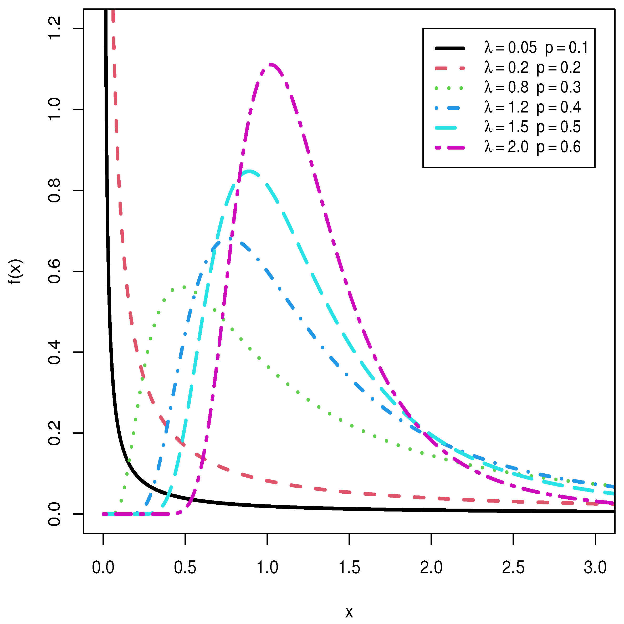
Figure 1, Figure 2, Figure 3 and Figure 4 show the forms of the FB pdf and hrf using various specific parameter settings.

Figure 1. Different shapes of pdf for FB distribution at $\beta =1.5$ and $n=5$.

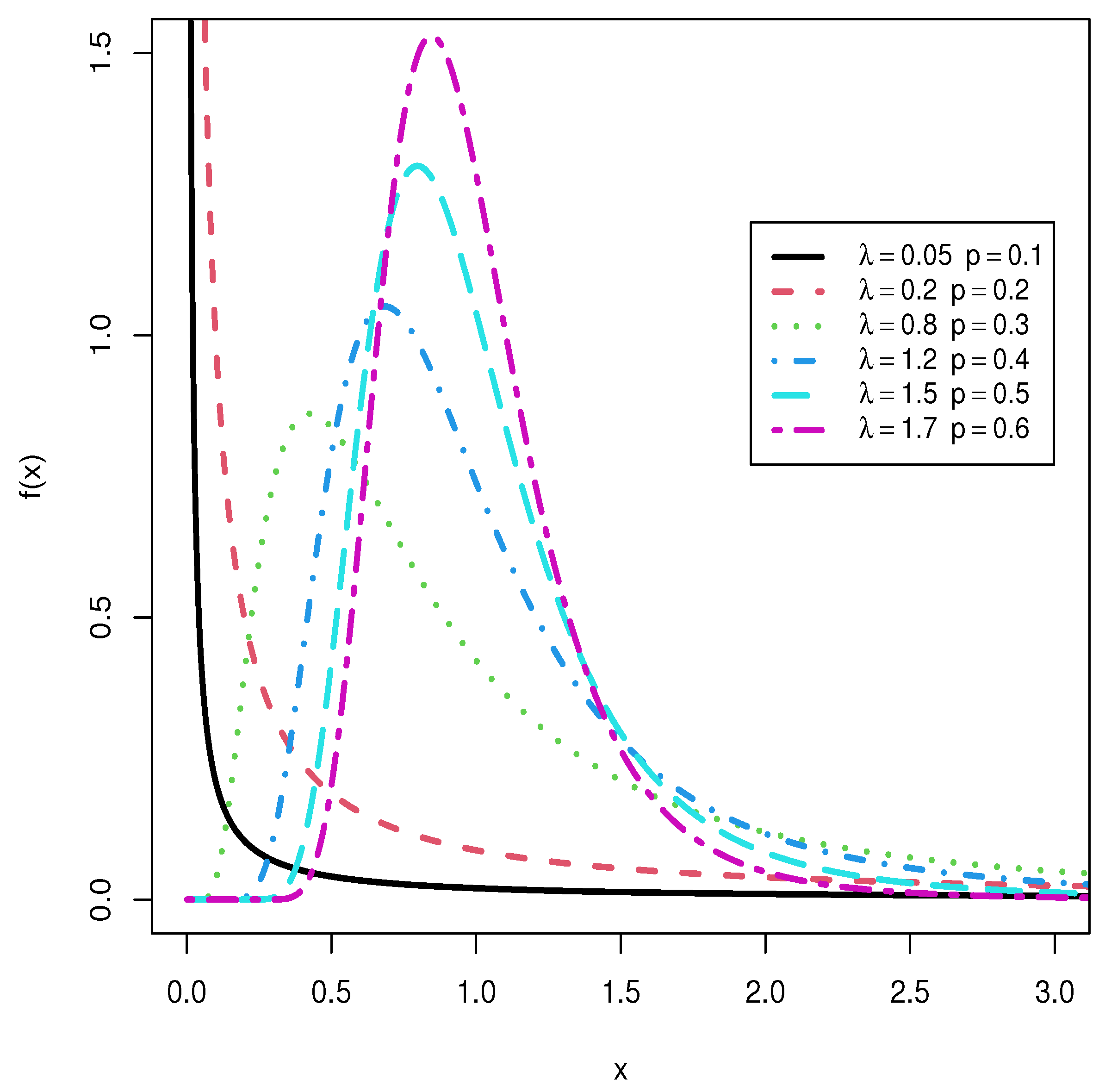
Figure 2. Different shapes of pdf for FB distribution at $\beta =1.5$ and $n=10$.

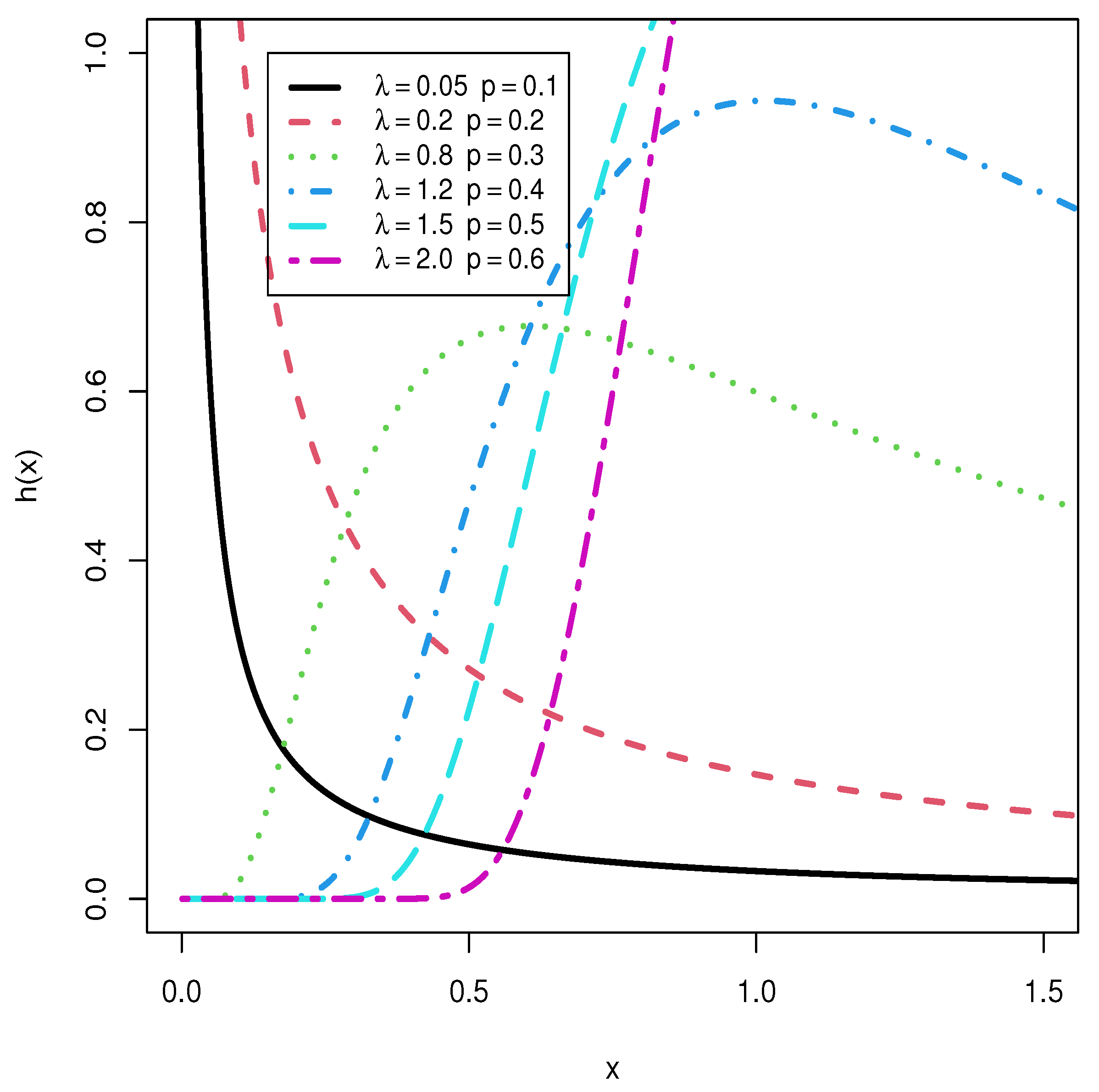
Figure 3. Different shapes of hrf for FB distribution at $\beta =1.5$ and $n=5$.

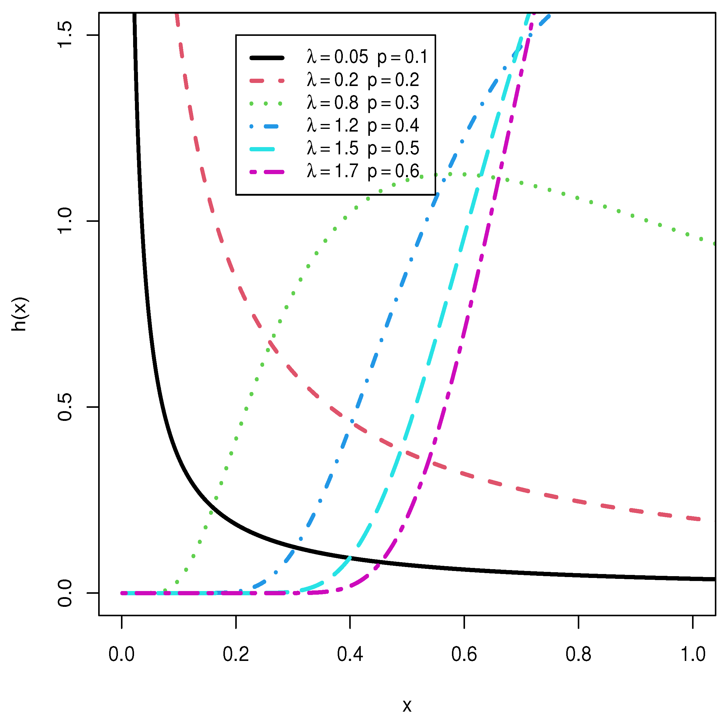
Figure 4. Different shapes of hrf for FB distribution at $\beta =1.5$ and $n=10$.

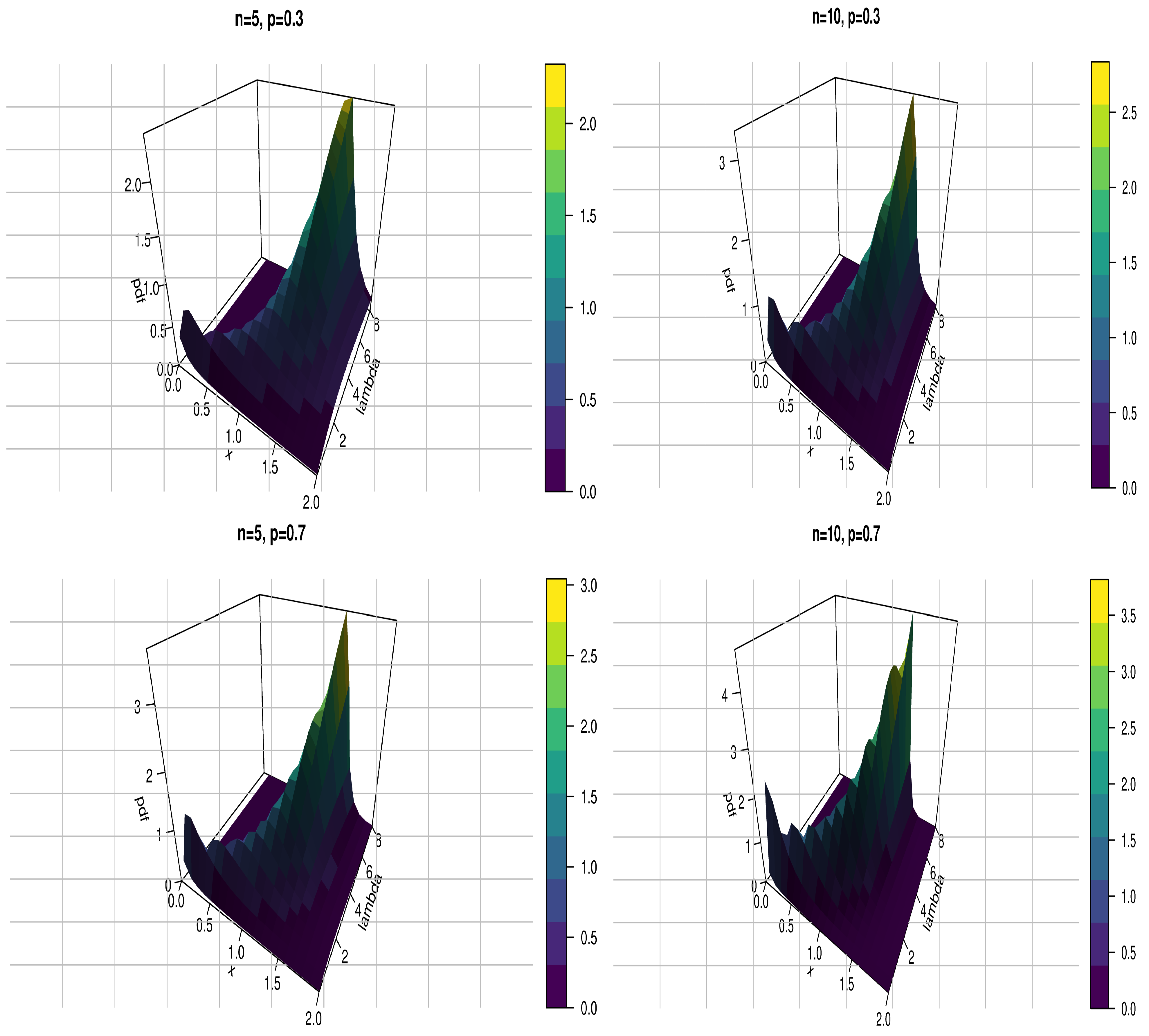
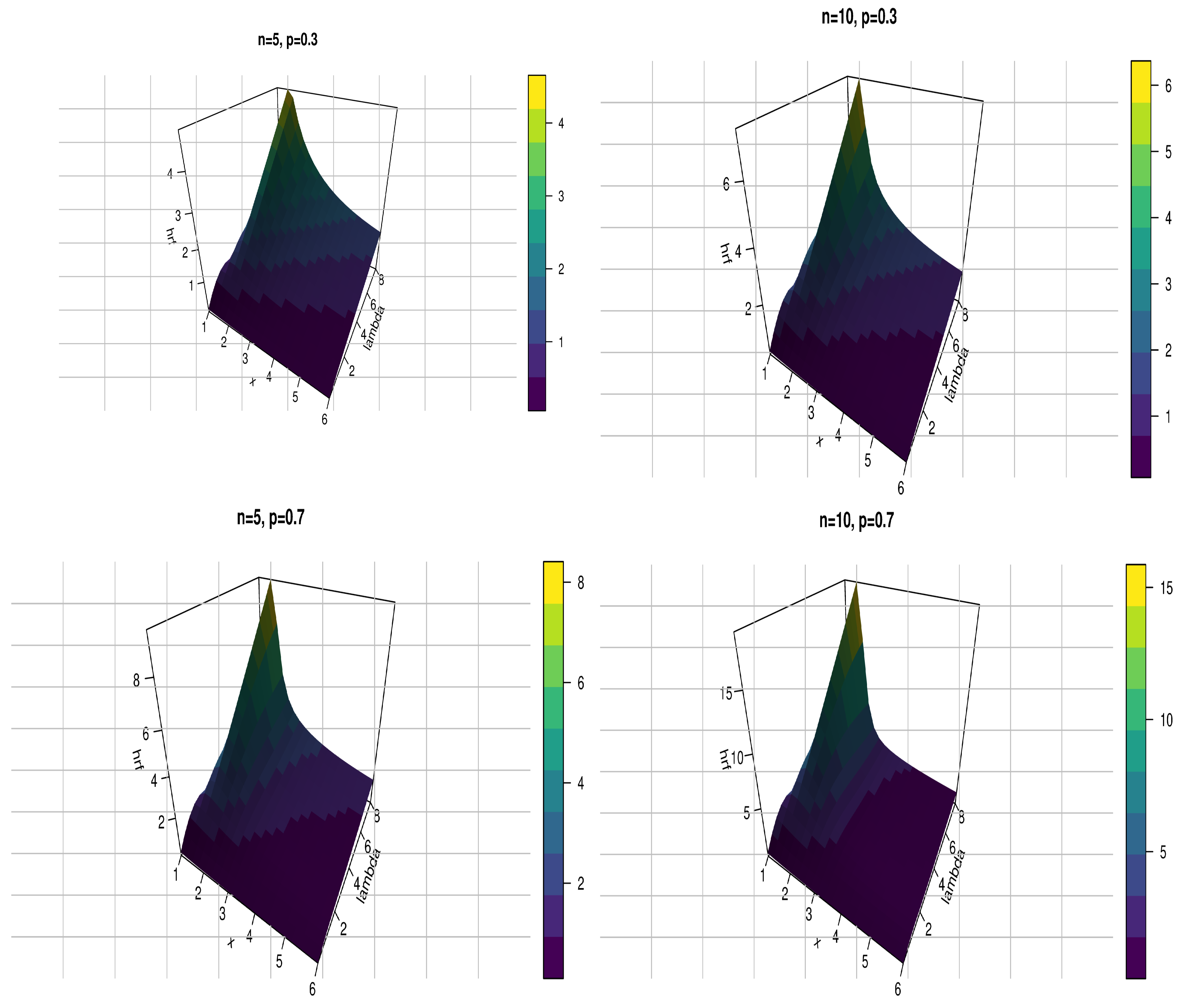
Figure 1 and Figure 2 illustrate that the pdf of the FB distribution can be unimodal, decreasing and skewed to the right. Figure 3 and Figure 4 display that the hrf of the FB distribution includes increasing, decreasing, upside-down and reversed-J form. Furthermore, Figure 5 and Figure 6 represent the 3D plots of the FB pdf and hrf using various specific parameter settings. Furthermore, Figure 5 and Figure 6 support the above comments for the pdf and hrf of FB distribution.

Figure 5. Three-dimensional different shapes of pdf for FB distribution at $\beta =1.5$.

Figure 6. Three-dimensional different shapes of hrf for FB distribution at $\beta =1.5$.

The FB distribution has a good motivation for unit failure, or system or device failures, among which device failure occurs due to an unknown number N of initial defects of the same type. Allow the $R_V$s Ws to explain their lives, and every fault can only be identified after producing a failure, in which case it is properly corrected. Assuming that the Ws are $R_V$s independent of N, which follow FB distribution, then the FB distribution accurately models the time to the first failure. Indeed, in reliability theory, the $R_V$$X=min{\left\{W_i\right\}}_{i=1}^N$ can indeed be utilized in serial systems with equivalent items, which are used in a wide range of industrial applications and biological organisms.

The quality of a product is vital to long-term customers, but the product’s owners or manufacturers are interested in reducing costs and time in the manufacturing process. These goals have prompted researchers in the field to develop a method for maintaining the quality of product batches. Acceptance sampling strategies are widely used in the industry to highlight the acceptability of a lot based on a random sample of the product. The consumer can accept or reject the lot based on this sample. The ACS method begins by obtaining the minimum adequate size that is required to highlight a certain percentile or average life when the life test is terminated at a pre-specified period. These examinations are known as abbreviated lifespan tests. ACS is one of the oldest quality assurance procedures and is focused on inspection and decision making for large quantities of products. The following is an example of an ACS application:

• Required: A vendor sends a shipment of items to a corporation. This product is frequently a component or raw material utilized in the production process of the company.
• Sampling: The relevant quality characteristic of the units in the sample is examined when a sample is obtained from the batch.
• Decision: Based on the information from the presented sample, a judgment is made on whether to accept or reject the lot.
  • Acceptable lots are placed into production for accepted samples.
  • Regarding rejected samples: Rejected lots may be returned to the vendor or subjected to another lot disposition procedure.

In the article under consideration, our primary focus lies in introducing a new lifetime distribution by composing the binomial family and the Fréchet distribution. This new lifetime model is called Fréchet binomial distribution. The following arguments give enough motivation to study the proposed model. We specify it as follows: (i) the new suggested distribution is very flexible and contains some distributions as sub-models; (ii) the shapes of the pdf for the new model can be unimodal, decreasing and skewed to the right. Furthermore, the shapes of the hrf for the suggested model can be increasing, decreasing, upside-down and reversed-J; (iii) the new suggested model has a closed form for quantile function and this makes the calculation of some properties such as skewness and kurtosis very easy; also to generate random numbers from the new suggested model becomes easy; (iv) some statistical and mathematical properties of the new suggested model are explored; (v) acceptance sampling plan for the new suggested model is discussed; (vi) maximum likelihood method of estimation is produced to estimate the parameters of the FB model; (vii) we hope that the proposed model can be implemented to fit data in diverse scientific entities. This ability of the model is explored using three real life datasets. The new suggested model is compared with eight known statistical models, namely odd Perks exponential (OPE); power Lomax (PL); alpha power inverse Weibull (APIW); exponentiated Weibull (Exp-W); extended Weibull (Ext-W); odd Weibull inverse Topp–Leone (OWITL); alpha power Lomax (APL); Marshall–Olkin Lomax (MOL); and generalization length biased exponential (GLBE) distributions. The new suggested model offers a significantly superior fit.

This article is arranged as described in the following: In Section 2, we presented a useful mixture for FB pdf and cdf, as well as sub-models of this distribution. Several statistical and mathematical features of FB distribution are provided in Section 3. A single ACS plan is proposed in Section 4. In Section 5, the parameter estimation of FB distribution is performed using the maximum likelihood method. The simulation study was performed to assess the behavior of estimates in Section 6. The applications to three real datasets investigate the flexibility of the proposed distribution in Section 7. Finally, concluding remarks are mentioned.

2. Important Mixture Representation and Sub-Models

2.1. The Mixture Representation

In this subsection, we derived the density expansion of the FB distribution. If $a>0$ is a real non-integer and $\mid o\mid <1,$ the binomial expansion holds

$${(1-o)}^{a-1}=\sum _{j=0}^{\infty }{(-1)}^j\left(\genfrac{}{}{0pt}{}{a-1}{j}\right)o^j,$$

(6)

applying (6) in (5) gives

$$\begin{array}{ccc}\hfill f(x;\lambda ,\beta ,p)& =& \frac{n{p}^{i+1}\lambda {\beta }^{\lambda }}{1-{\overline{p}}^n}\sum _{i=0}^{n-1}{(-1)}^i\left(\genfrac{}{}{0pt}{}{n-1}{i}\right)x^{-\lambda -1}{e}^{-(i+1){\left(\frac{\beta }{x}\right)}^{\lambda }}\hfill \\ & & \hfill \\ & =& \sum _{i=0}^{n-1}{\varpi }_i{\pi }_{(i+1)}\left(x\right)\hfill \end{array}$$

(7)

where

$${\varpi }_i=\frac{n}{(1-{\overline{p}}^n)}\sum _{i=0}^{n-1}\frac{{(-1)}^i}{(i+1)}\left(\genfrac{}{}{0pt}{}{n-1}{i}\right)p^{i+1},$$

and ${\pi }_{(i+1)}\left(x\right)$ is the F pdf with the scale parameter $\beta {(i+1)}^{\frac{1}{\lambda }}$ and shape parameter $\lambda$. As a result, the FB pdf may be written as a linear mixture of F pdfs. As a result, some mathematical and statistical features of the FB distribution are directly derived from those of Equation (7) and the F distribution. Similarly, the cdf of the FB distribution can also be expressed as

$$F(x;\lambda ,\beta ,p)=\sum _{i=0}^{n-1}{\varpi }_i{\mathsf{\Pi }}_{(i+1)}\left(x\right)$$

(8)

where ${\mathsf{\Pi }}_{(i+1)}\left(x\right)$ is the F cdf with the scale parameter $\beta {(i+1)}^{\frac{1}{\lambda }}$ and shape parameter $\lambda .$

2.2. Sub-Models of the FB Model

The FB is a very adaptable and flexible model which contains several continuous statistical models when its parameters are changed. If X is a $R_V$ with cdf (4), using the notation $X\sim FB(\lambda ,\beta ,p)$ then we have the following cases: 1—When $\beta =1$, we obtain the inverse exponential binomial model (new); 2—At $\beta =2,$ we obtain the inverse Rayleigh binomial model (new); 3—If $n=1$(or $p⟶0)$, $\beta =1$, we obtain the inverse exponential model; 4—If $n=1$(or $p⟶0)$, $\beta =2$, we obtain the inverse Rayleigh model; 5—When $\beta =q$$c^{\frac{1}{\lambda }}$, we obtain generalized inverse Weibull binomial model (new); 6—If $n=1$(or $p⟶0)$, we have F distribution which is defined by [1].

3. Statistical and Mathematical Features

In this section, we investigate different statistical and mathematical features of the FB model including the $Q_{UN}F$, $M_O$, $I{M}_O$, $C{M}_O$, $M_{O}GF$, $PW{M}_O$, order statistics and Rényi entropy.

3.1. Quantile Function

$Q_{UN}F$s are employed in theoretical aspects, statistical applications and Monte Carlo approaches. The FB $Q_{UN}F$ can be obtained by inverting (6) as follows

$$F^{-1}\left(u\right)=x_u=\beta {\left\{-\log \frac{1}{p}\left[1-{\left[1-u(1-{\overline{p}}^n)\right]}^{\frac{1}{n}}\right]\right\}}^{\frac{-1}{\lambda }},$$

(9)

where $Q_{G\left(u\right)}$ symbolizes the $Q_{UN}F$ corresponding to $G\left(x\right)$. The median M can be computed by putting $u=0.5$ as

$$M=\beta {\left\{-\log \frac{1}{p}\left[1-{\left[1-0.5(1-{\overline{p}}^n)\right]}^{\frac{1}{n}}\right]\right\}}^{\frac{-1}{\lambda }}.$$

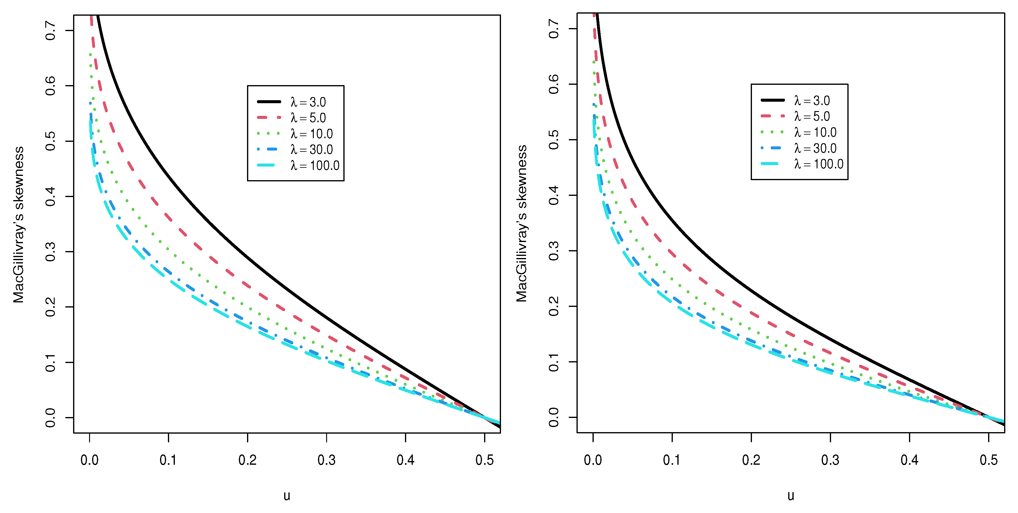
The MacGillivray’s skewness ($MSK$) function [28] is calculated via

$$MSK=\frac{x_u+x_{1-u}-2x_{0.5}}{x_u-x_{1-u}},0<u<1.$$

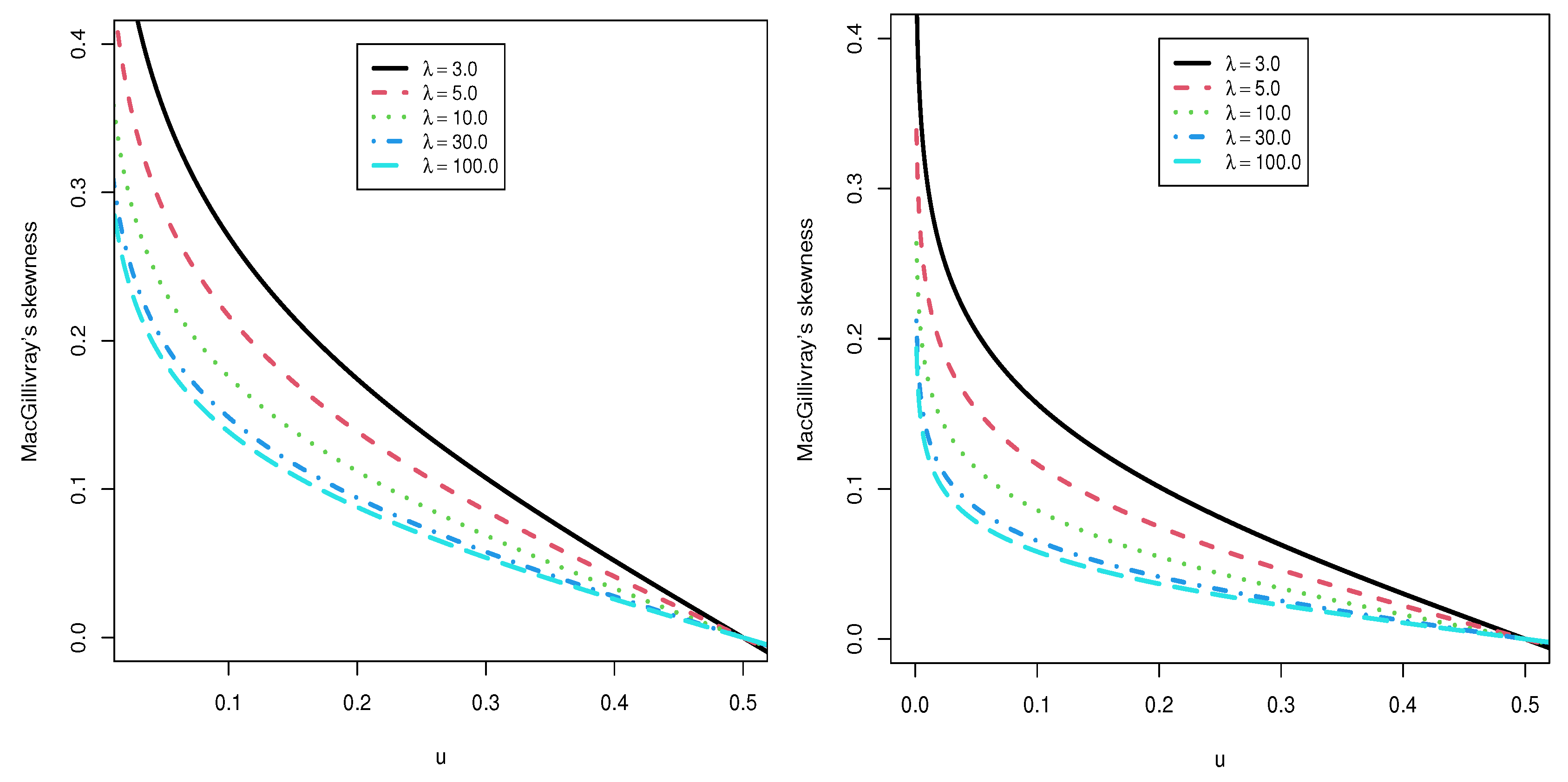
Figure 7 and Figure 8 display the plots of MacGillivray’s skewness at $\beta =0.5$ and for some values of the parameters. We can see that the magnitude of MacGillivray’s skewness decreases as $\lambda$ increases.

Figure 7. Plots of the MacGillivray’s skewness for FB distribution at $p=0.3$ and $n=5,10$.

Figure 8. Plots of the MacGillivray’s skewness for FB distribution at $p=0.7$ and $n=5,10$.

3.2. Moments and Moment-Generating Functions

In this subsection, we will present the $r_{th}$$M_O$s and $M_{O}GF$s of FB distribution. $M_O$s are very useful in statistical analysis and are useful for measuring skewness and kurtosis and providing clear information about the shape of the distribution. If X has pdf (5), then the $r_{th}$$M_O$ of X is provided via

$${\mu }_r^{{}^{\prime }}={\int }_0^{\infty }{x}^{r}f\left(x\right)dx=\frac{n{p}^{i+1}{\beta }^{\lambda }}{1-{\overline{p}}^n}\sum _{i=0}^{n-1}{(-1)}^i\left(\genfrac{}{}{0pt}{}{n-1}{i}\right){\int }_0^{\infty }{x}^{r-\lambda -1}{e}^{-(i+1){\left(\frac{\beta }{x}\right)}^{\lambda }}dx.$$

By setting $y=(i+1)\frac{\beta }{x},$ after some algebra, $r_{th}$$M_O$ takes the following form

$${\mu }_r^{{}^{\prime }}=\frac{n{\beta }^r}{1-{\overline{p}}^n}\sum _{i=0}^{n-1}\frac{{(-1)}^i\left(\genfrac{}{}{0pt}{}{n-1}{i}\right)p^{i+1}}{{(i+1)}^{1-\frac{r}{\lambda }}}\mathsf{\Gamma }(1-\frac{r}{\lambda }),\frac{r}{\lambda }<1.$$

(10)

Table 1 and Table 2 show the numerical values of $E\left(X\right)$, $E\left(X^2\right)$, $E\left(X^3\right)$, $E\left(X^4\right)$, variance (V), skewness (SK), kurtosis (KU) and coefficient of variation (CV) of the FB distribution.

Table 1. Results of ${\mu }_1^{{}^{\prime }}$, ${\mu }_2^{{}^{\prime }}$, ${\mu }_3^{{}^{\prime }}$, ${\mu }_4^{{}^{\prime }}$, V, $CS$, $CK$ and $CV$ for the $FB$ model at $\beta$ = 0.5 and n = 5.

$\mathit{\lambda }\downarrow$	$\mathit{p}\downarrow$	${\mathit{\mu }}_1^{{}^{\prime }}\uparrow$	${\mathit{\mu }}_2^{{}^{\prime }}\uparrow$	${\mathit{\mu }}_3^{{}^{\prime }}\uparrow$	${\mathit{\mu }}_4^{{}^{\prime }}\uparrow$	$\mathit{V}\uparrow$	$\mathit{C}\mathit{S}\downarrow$	$\mathit{C}\mathit{K}\downarrow$	$\mathit{C}\mathit{V}\downarrow$
	0.3	6.507	261.036	16,080	1,160,000	218.69	3.568	16.785	2.273
	0.4	6.904	250.87	14,900	1,057,000	203.211	3.577	17.21	2.065
5	0.5	6.959	227.599	12,990	905,600	179.17	3.714	18.791	1.923
	0.6	6.849	200.84	10,980	752,200	153.932	3.923	21.162	1.812
	0.7	6.67	175.099	9143	615,600	130.613	4.176	24.177	1.713
	0.3	4.809	172.585	10,290	731,700	149.458	4.39	24.898	2.542
	0.4	4.938	152.52	8629	600,100	128.14	4.557	27.421	2.293
7	0.5	4.899	129.259	6902	469,200	105.262	4.849	31.663	2.094
	0.6	4.808	108.238	5428	360,600	85.125	5.206	37.215	1.919
	0.7	4.712	90.876	4260	276,700	68.673	5.597	43.899	1.759
	0.3	3.425	107.512	6172	432,100	95.78	5.492	38.658	2.857
	0.4	3.48	88.029	4697	319,300	75.918	5.838	45.092	2.504
9	0.5	3.477	70.442	3457	228,000	58.352	6.296	54.224	2.197
	0.6	3.473	56.753	2537	162,300	44.689	6.795	65.475	1.925
	0.7	3.483	46.66	1884	116,900	34.53	7.299	78.482	1.687
	0.3	2.413	64.529	3547	243,900	58.707	6.908	61.474	3.175
	0.4	2.485	49.444	2456	162,600	43.27	7.44	74.75	2.648
11	0.5	2.553	37.921	1670	106,200	31.402	8.027	91.814	2.195
	0.6	2.636	29.99	1150	70,130	23.043	8.58	111.331	1.821
	0.7	2.729	24.724	812.468	47,420	17.277	9.061	132.308	1.523
	0.3	1.713	37.896	1980	133,500	34.963	8.682	98.68	3.453
	0.4	1.828	27.534	1252	80,430	24.193	9.352	122.661	2.691
13	0.5	1.962	20.658	790.31	48,120	16.81	9.922	149.874	2.09
	0.6	2.108	16.466	514.301	29,510	12.021	10.291	176.814	1.644
	0.7	2.258	14.007	349.659	18,780	8.909	10.447	201.212	1.322
	0.3	1.24	22.016	1083	71,530	20.479	10.848	158.205	3.65
	0.4	1.396	15.431	628.342	38,970	13.48	11.499	196.064	2.629
15	0.5	1.577	11.625	371.251	21,400	9.136	11.736	230.168	1.916
	0.6	1.766	9.625	231.04	12,220	6.507	11.511	253.611	1.445
	0.7	1.95	8.677	153.722	7341	4.875	10.943	264.953	1.132
	0.3	0.922	12.76	585.088	37,710	11.909	13.415	251.07	3.742
	0.4	1.109	8.816	313.114	18,620	7.585	13.715	300.511	2.483
17	0.5	1.32	6.873	174.958	9409	5.131	13.109	324.741	1.716
	0.6	1.533	6.081	105.991	5021	3.729	11.833	319.237	1.259
	0.7	1.738	5.906	70.858	2863	2.887	10.309	293.974	0.978
	0.3	0.707	7.429	313.253	19,640	6.929	16.349	391.114	3.722
	0.4	0.913	5.194	155.873	8811	4.36	15.726	434.826	2.286
19	0.5	1.141	4.321	83.617	4112	3.019	13.686	412.427	1.523
	0.6	1.368	4.163	50.595	2063	2.292	11.134	346.881	1.107
	0.7	1.584	4.37	35.22	1126	1.862	8.818	273.93	0.862

Table 2. Results of ${\mu }_1^{{}^{\prime }}$, ${\mu }_2^{{}^{\prime }}$, ${\mu }_3^{{}^{\prime }}$, ${\mu }_4^{{}^{\prime }}$, V, $CS$, $CK$ and $CV$ for the $FB$ model at $\beta$ = 0.5 and n = 10.

$\mathit{\lambda }\downarrow$	$\mathit{p}\downarrow$	${\mathit{\mu }}_1^{{}^{\prime }}\uparrow$	${\mathit{\mu }}_2^{{}^{\prime }}\uparrow$	${\mathit{\mu }}_3^{{}^{\prime }}\uparrow$	${\mathit{\mu }}_4^{{}^{\prime }}\uparrow$	$\mathit{V}\uparrow$	$\mathit{C}\mathit{S}\downarrow$	$\mathit{C}\mathit{K}\downarrow$	$\mathit{C}\mathit{V}\downarrow$
	0.3	8.271	343.901	21,330	1,543,000	275.492	3.047	12.705	2.007
	0.4	9.46	365.459	21,920	1,559,000	275.966	2.888	11.845	1.756
5	0.5	10.179	364.457	21,050	1,471,000	260.841	2.857	11.88	1.587
	0.6	10.585	350.876	19,460	1,334,000	238.842	2.897	12.419	1.46
	0.7	10.789	331.229	17,590	1,182,000	214.824	2.981	13.296	1.358
	0.3	6.612	248.718	14,930	1,064,000	205.006	3.604	17.34	2.166
	0.4	7.396	248.367	14,190	988,300	193.665	3.521	17.09	1.882
7	0.5	7.854	235.163	12,710	863,000	173.471	3.561	17.925	1.677
	0.6	8.121	217.281	11,050	730,200	151.326	3.665	19.404	1.515
	0.7	8.28	198.934	9471	608,500	130.38	3.805	21.331	1.379
	0.3	5.067	169.461	9804	687,400	143.782	4.343	24.804	2.366
	0.4	5.637	160.199	8641	587,300	128.425	4.322	25.466	2.01
9	0.5	6.009	145.53	7241	475,500	109.423	4.413	27.481	1.741
	0.6	6.276	130.785	5947	376,000	91.402	4.553	30.282	1.523
	0.7	6.485	117.969	4866	295,400	75.914	4.712	33.591	1.344
	0.3	3.816	111.208	6166	424,600	96.646	5.267	36.355	2.576
	0.4	4.294	100.459	5057	334,300	82.02	5.279	38.283	2.109
11	0.5	4.667	88.754	3985	251,400	66.973	5.375	41.726	1.754
	0.6	4.983	78.922	3114	186,300	54.087	5.485	45.843	1.476
	0.7	5.265	71.509	2455	138,300	43.788	5.58	50.187	1.257
	0.3	2.871	71.364	3768	254,400	63.122	6.382	53.815	2.767
	0.4	3.322	62.327	2887	184,800	51.292	6.368	57.107	2.156
13	0.5	3.725	54.461	2154	129,400	40.584	6.376	61.494	1.71
	0.6	4.097	48.901	1617	90,160	32.117	6.337	65.674	1.383
	0.7	4.44	45.44	1244	63,580	25.724	6.236	69.062	1.142
	0.3	2.182	45.257	2258	149,100	40.496	7.692	79.648	2.916
	0.4	2.632	38.764	1625	100,200	31.837	7.544	83.434	2.144
15	0.5	3.068	34.17	1157	65,530	24.759	7.31	86.454	1.622
	0.6	3.483	31.647	845.752	43,120	19.516	6.955	87.162	1.268
	0.7	3.871	30.707	646.533	29,060	15.722	6.512	85.505	1.024
	0.3	1.688	28.586	1335	86,030	25.739	9.191	116.953	3.006
	0.4	2.142	24.424	908.132	53,610	19.835	8.726	118.023	2.079
17	0.5	2.603	22.187	624.565	32,870	15.414	8.04	114.211	1.509
	0.6	3.047	21.6	452.158	20,560	12.313	7.204	105.458	1.151
	0.7	3.465	22.138	351.553	13,370	10.135	6.342	94.02	0.919
	0.3	1.333	18.097	782.914	49,070	16.32	10.849	169.239	3.03
	0.4	1.791	15.724	507.221	28,430	12.518	9.804	159.957	1.976
19	0.5	2.266	15.029	341.755	16,430	9.896	8.444	140.09	1.388
	0.6	2.728	15.584	250.519	9850	8.141	7.043	115.373	1.046
	0.7	3.163	16.933	203.291	6267	6.928	5.808	91.909	0.832

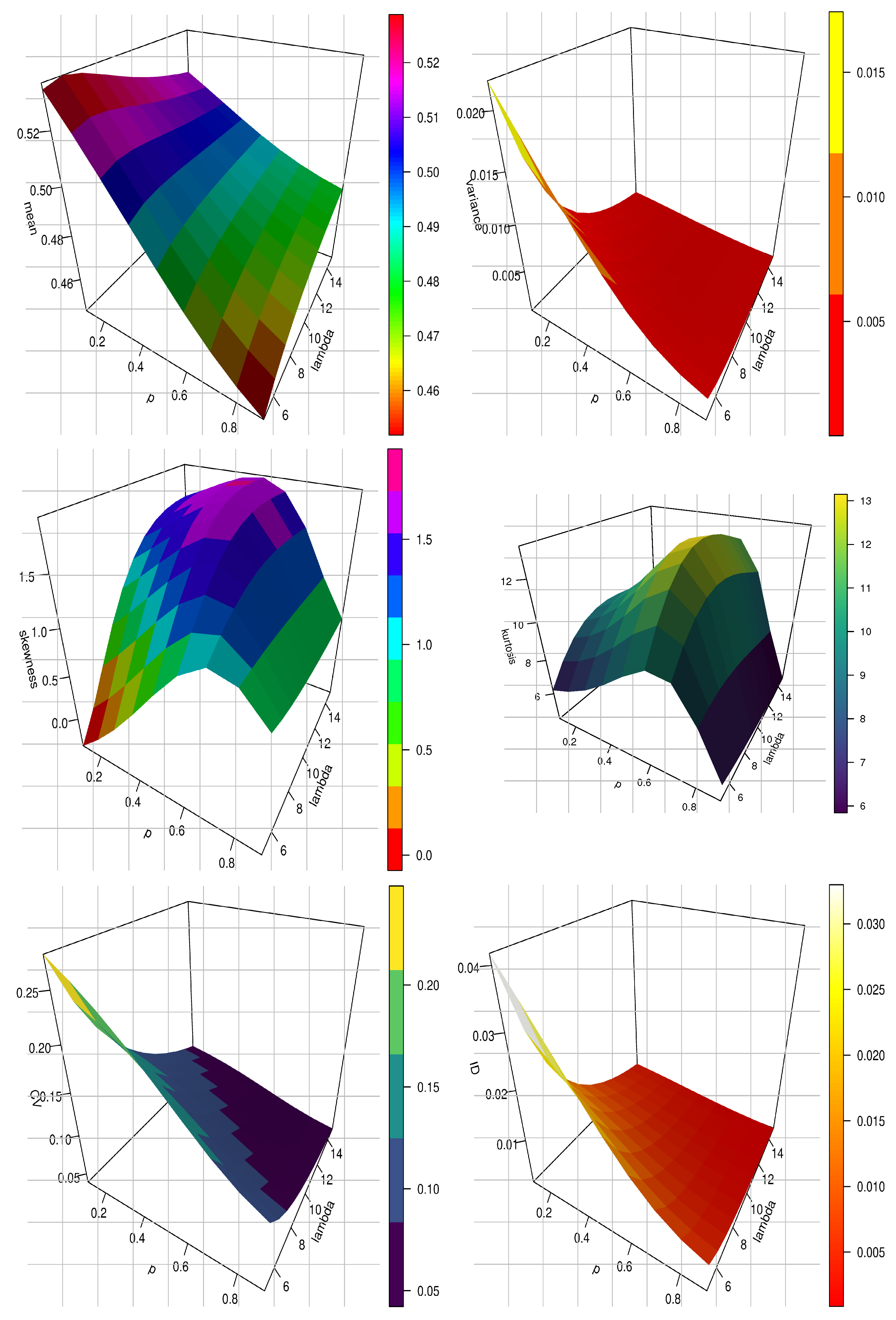
Figure 9 and Figure 10 represent the 3D plots of the mean, variance, CS, CK, CV and index of dispersion (ID) for the FB model at $p\in [0,1],\lambda \in [5,15]$ and $n=5,10$.

Figure 9. 3D plots of mean, variance, CS, CK, CV and ID for FB Model at $p\in [0,1],\lambda \in [5,15]$ and $n=5$.

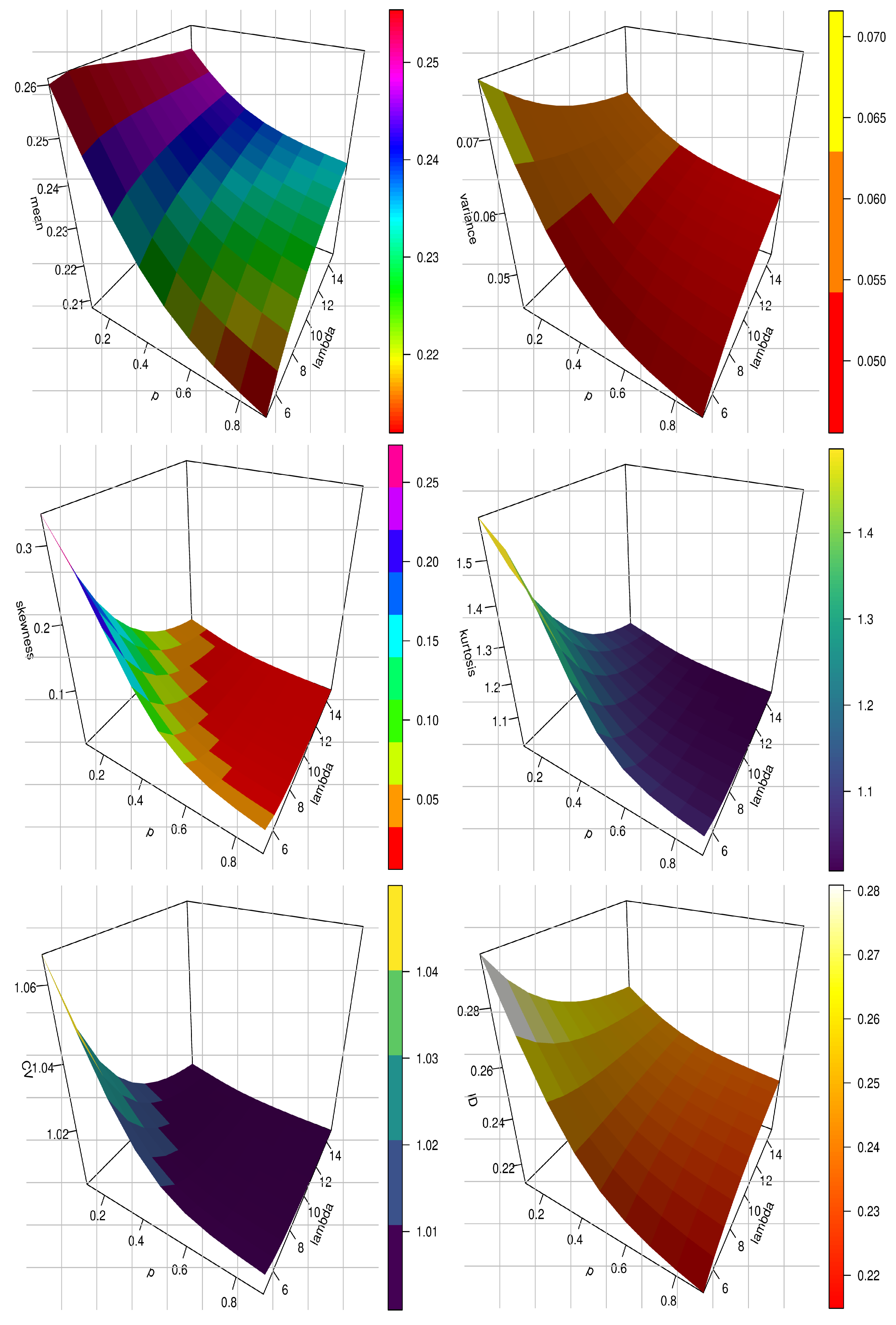
Figure 10. Three-dimensional plots of the mean, variance, CS, CK, CV and ID for FB model at $p\in [0,1],\lambda \in [5,15]$ and $n=10$.

The $M_{O}GF$$M_X\left(t\right)$ of X may be calculated using (5) as follows:

$$M_X\left(t\right)=E\left(e^{tX}\right)=\frac{n{\beta }^r}{1-{\overline{p}}^n}\sum _{r=0}^{\infty }\sum _{i=0}^{n-1}\frac{t^r}{r!}\frac{{(-1)}^i\left(\genfrac{}{}{0pt}{}{n-1}{i}\right)p^{i+1}}{{(i+1)}^{1-\frac{r}{\lambda }}}.$$

(11)

3.3. Upper and Lower Incomplete Moments

The $s_{th}$ upper (U) and lower (L) $I{M}_O$s of X are represented by ${\mathsf{\Psi }}_s\left(t\right)=E(X^s\mid X>t)={\int }_t^{\infty }{x}^s$$f\left(x\right)dx$ and ${\mathsf{\Omega }}_s\left(t\right)=E(X^s\mid X<t)={\int }_0^t{x}^{s}f\left(x\right)dx$, respectively, for any real $s>0.$ The $s_{th}$ U $I{M}_O$ of the FB distribution can be computed with

$$\begin{array}{ccc}\hfill {\mathsf{\Psi }}_s\left(t\right)& =& \frac{n{p}^{i+1}\lambda {\beta }^{\lambda }}{1-{\overline{p}}^n}\sum _{i=0}^{n-1}{(-1)}^i\left(\genfrac{}{}{0pt}{}{n-1}{i}\right){\int }_t^{\infty }{x}^{s-\lambda -1}{e}^{-(i+1){\left(\frac{\beta }{x}\right)}^{\lambda }}dx\hfill \\ & & \hfill \\ & =& \frac{n{\beta }^s}{1-{\overline{p}}^n}\sum _{i=0}^{n-1}\frac{{(-1)}^i\left(\genfrac{}{}{0pt}{}{n-1}{i}\right)p^{i+1}}{{(i+1)}^{1-\frac{s}{\lambda }}}\mathsf{\Gamma }(1-\frac{s}{\lambda },(i+1){\left(\frac{\beta }{t}\right)}^{\lambda }).\hfill \end{array}$$

(12)

In the same way, the $s_{th}$ L $I{M}_O$ of the FB distribution is computed with

$$\begin{array}{ccc}\hfill {\mathsf{\Omega }}_s\left(t\right)& =& \frac{n{p}^{i+1}\lambda {\beta }^{\lambda }}{1-{\overline{p}}^n}\sum _{i=0}^{n-1}{(-1)}^i\left(\genfrac{}{}{0pt}{}{n-1}{i}\right){\int }_0^t{x}^{s-\lambda -1}{e}^{-(i+1){\left(\frac{\beta }{x}\right)}^{\lambda }}dx\hfill \\ & & \hfill \\ & =& \frac{n{\beta }^s}{1-{\overline{p}}^n}\sum _{i=0}^{n-1}\frac{{(-1)}^i\left(\genfrac{}{}{0pt}{}{n-1}{i}\right)p^{i+1}}{{(i+1)}^{1-\frac{s}{\lambda }}}\gamma (1-\frac{s}{\lambda },(i+1){\left(\frac{\beta }{t}\right)}^{\lambda })\hfill \end{array}$$

(13)

where $\mathsf{\Gamma }(s,t)={\int }_t^{\infty }{x}^{s-1}{e}^{-x}dx$ and $\gamma (s,t)={\int }_0^t{x}^{s-1}{e}^{-x}dx$ are the U and L incomplete gamma function, respectively.

The mean deviation about the mean, and about the M, are calculated with ${\delta }_{\mu }\left(x\right)=2{\mu }_1^{{}^{\prime }}F$$\left({\mu }_1^{{}^{\prime }}\right)-2{\mathsf{\Omega }}_1\left({\mu }_1^{{}^{\prime }}\right)$ and ${\delta }_M\left(x\right)={\mu }_1^{{}^{\prime }}-2{\mathsf{\Omega }}_1\left(M\right)$, respectively, where F$\left({\mu }_1^{{}^{\prime }}\right)$ is computed from (4) and ${\mathsf{\Omega }}_s\left(t\right)$ is the first $I{M}_O$ when put $s=1$ in (13), we obtain

$${\mathsf{\Omega }}_1\left(t\right)=\frac{n{p}^{i+1}{\beta }^{\lambda }}{1-{\overline{p}}^n}\sum _{i=0}^{n-1}{(-1)}^i\left(\genfrac{}{}{0pt}{}{n-1}{i}\right)\frac{\gamma (1-\frac{1}{\lambda },(i+1){\left(\frac{\beta }{t}\right)}^{\lambda })}{{(i+1)}^{1-\frac{1}{\lambda }}}.$$

3.4. Probability Weighted Moments

For an $R_V$X, the ${(r,s)}_{th}$$PW{M}_O$ can be computed as follows

$${\rho }_{r,s}=E\left[X^{r}F{\left(x\right)}^s\right]={\int }_0^{\infty }{x}^{r}F{\left(x\right)}^{s}f\left(x\right)dx.$$

Using (4) and (5), we can write

$$\begin{array}{ccc}\hfill {\rho }_{r,s}& =& \frac{np\lambda {\beta }^{\lambda }}{{(1-{\overline{p}}^n)}^{s+1}}{\int }_0^{\infty }{x}^{r-\lambda -1}{e}^{-{\left(\frac{\beta }{x}\right)}^{\lambda }}{\left[1-p{e}^{-{\left(\frac{\beta }{x}\right)}^{\lambda }}\right]}^{n-1}\hfill \\ & & \\ & & \times {\left\{1-{\left[1-p{e}^{-{\left(\frac{\beta }{x}\right)}^{\lambda }}\right]}^{n-1}\right\}}^{s}dx,\hfill \end{array}$$

using (6), and after minor algebraic reduction, the ${(r,s)}_{th}$$PW{M}_O$ can be derived as

$${\rho }_{r,s}=\sum _{i,j=0}^{\infty }\frac{p^{j+1}{(-1)}^{i+j}}{{(j+1)}^{1-\frac{r}{\lambda }}}\left(\genfrac{}{}{0pt}{}{s}{i}\right)\left(\genfrac{}{}{0pt}{}{n(i+1)-1}{j}\right)\frac{n{\beta }^r}{{(1-{\overline{p}}^n)}^{s+1}}\mathsf{\Gamma }(1-\frac{r}{\lambda }).$$

3.5. Order Statistics

Order statistics have several applications in survival, reliability and failure analysis, and they are a logical technique to undertake a system reliability study. The $M_O$s of order statistics are critical in testing for dependability and quality control see [29]. Assume $X_1$, $X_2$,..., $X_n$ be a random sample from FB distribution of size n and $X_{(1;n)}\le$$X_{(2;n)}\le \dots ,\le$$X_{(n;n)}$ are ordered statistics of $R_S$. The pdf of $X_{(i;n)},$$i=1,2,\dots ,n$ can indeed be expressed as

$$f_{i;n}\left(x\right)=\frac{f\left(x\right)}{B(i,n-i+1)}\sum _{j=0}^{n-i}{(-1)}^j\left(\genfrac{}{}{0pt}{}{n-i}{j}\right)F^{i+j-1}\left(x\right).$$

(14)

Substituting (7) and (8) in (14), we obtain

$$\begin{array}{ccc}\hfill f_{i;n}\left(x\right)& =& \sum _{j=0}^{n-i}{(-1)}^j\left(\genfrac{}{}{0pt}{}{n-i}{j}\right)\frac{np\lambda {\beta }^{\lambda }{x}^{-\lambda -1}{e}^{-{\left(\frac{\beta }{x}\right)}^{\lambda }}{\left[1-p{e}^{-{\left(\frac{\beta }{x}\right)}^{\lambda }}\right]}^{n-1}}{B(i,n-i+1){(1-{\overline{p}}^n)}^{i+j}}\hfill \\ & & \hfill \\ & & \times {\left[1-{\left[1-p{e}^{-{\left(\frac{\beta }{x}\right)}^{\lambda }}\right]}^n\right]}^{i+j-1},\hfill \end{array}$$

(15)

using (6), and after some algebraic simplification, the pdf of the $i_{th}$ order statistics can indeed be expressed as

$$\begin{array}{ccc}\hfill f_{i;n}\left(x\right)& =& \sum _{k,d=0}^{\infty }\sum _{j=0}^{n-i}\frac{{(-1)}^{j+k+d}n{p}^{d+1}\lambda {\beta }^{\lambda }}{B(i,n-i+1){(1-{\overline{p}}^n)}^{i+j}}\left(\genfrac{}{}{0pt}{}{n-i}{j}\right)\left(\genfrac{}{}{0pt}{}{i+j-1}{k}\right)\left(\genfrac{}{}{0pt}{}{n(k+1)-1}{d}\right)\hfill \\ & & \hfill \\ & & \times x^{-\lambda -1}{e}^{-(d+1){\left(\frac{\beta }{x}\right)}^{\lambda }}.\hfill \end{array}$$

(16)

The $r_{th}$$M_O$ of the $i^{th}$ order statistics is provided via

$$\begin{array}{ccc}\hfill {\mu }_r& =& E\left(X_{i:r}^r\right)={\int }_0^{\infty }{x}^r{f}_{i;n}\left(x\right)dx=\hfill \\ & & \\ & =& \sum _{k,d=0}^{\infty }\sum _{j=0}^{n-i}\frac{{(-1)}^{j+k+d}n{p}^{d+1}\lambda {\beta }^{\lambda }}{B(i,n-i+1){(1-{\overline{p}}^n)}^{i+j}}\left(\genfrac{}{}{0pt}{}{n-i}{j}\right)\left(\genfrac{}{}{0pt}{}{i+j-1}{k}\right)\left(\genfrac{}{}{0pt}{}{n(k+1)-1}{d}\right)\hfill \\ & & \\ & & \times {\int }_0^{\infty }{x}^{r-\lambda -1}{e}^{-(d+1){\left(\frac{\beta }{x}\right)}^{\lambda }}\hfill \\ & & \\ & =& \sum _{k,d=0}^{\infty }\sum _{j=0}^{n-i}\frac{{(-1)}^{j+k+d}n{p}^{d+1}{\beta }^d}{B(i,n-i+1)}\left(\genfrac{}{}{0pt}{}{n-i}{j}\right)\left(\genfrac{}{}{0pt}{}{i+j-1}{k}\right)\left(\genfrac{}{}{0pt}{}{n(k+1)-1}{d}\right)\hfill \\ & & \\ & & \times \frac{\mathsf{\Gamma }(1-\frac{r}{\lambda })}{{(1-{\overline{p}}^n)}^{i+j}{(d+1)}^{1-\frac{r}{\lambda }}}.\hfill \end{array}$$

3.6. Entropy

The Rényi entropy is important in measuring the level of uncertainty associated with a $R_V$X. The Rényi entropy is determined by

$$I_R\left(\rho \right)=\frac{1}{1-\rho }\log \left[{\int }_0^{\infty }{f}^{\rho }\left(x\right)dx\right]\rho >0,\rho \ne 1.$$

(17)

From (5), we have

$${\int }_0^{\infty }{f}^{\delta }\left(x\right)dx={\left(\frac{np\lambda {\beta }^{\lambda }}{1-{\overline{p}}^n}\right)}^{\rho }{\int }_0^{\infty }{x}^{-\rho (\lambda +1)}{e}^{-\rho {\left(\frac{\beta }{x}\right)}^{\lambda }}{\left[1-p{e}^{-{\left(\frac{\beta }{x}\right)}^{\lambda }}\right]}^{\rho (n-1)},$$

using (6) and after some simplifications, we obtain

$$\begin{array}{ccc}\hfill {\int }_0^{\infty }{f}^{\delta }\left(x\right)dx& =& {\left(\frac{np\lambda {\beta }^{\lambda }}{1-{\overline{p}}^n}\right)}^{\rho }\sum _{i=0}^{\infty }{(-1)}^i\left(\genfrac{}{}{0pt}{}{\rho (n-1)}{i}\right)p^i\frac{{\beta }^{1-\rho (\lambda -1)}}{\lambda }\hfill \\ & & \\ & & \times \frac{\mathsf{\Gamma }(\rho +\frac{1}{\lambda }(\rho -1)}{{(i+\rho )}^{\rho +\frac{1}{\lambda }(\rho -1}}.\hfill \end{array}$$

Thus,

$$\begin{array}{ccc}\hfill I_R\left(\rho \right)& =& \frac{\rho }{1-\rho }\log \left(\frac{np\lambda {\beta }^{\lambda }}{1-{\overline{p}}^n}\right)\hfill \\ & & \hfill \\ & & +\frac{1}{1-\rho }\log \left\{\sum _{i=0}^{\infty }{(-1)}^i\left(\genfrac{}{}{0pt}{}{\rho (n-1)}{i}\right)p^i\frac{{\beta }^{1-\rho (\lambda -1)}}{\lambda }\frac{\mathsf{\Gamma }(\rho +\frac{1}{\lambda }(\rho -1)}{{(i+\rho )}^{\rho +\frac{1}{\lambda }(\rho -1}}\right\}.\hfill \end{array}$$

(18)

4. ACS Plan

We presume that a product’s lifespan follows the FB distribution with parameters $(\lambda ,\beta ,p)$ described by (4), and as such, the stated median lifetime of the units claimed by a manufacturer is $m_0$. Based on the criterion that the actual median lifetime of the units, m, is greater than the required lifetime $m_0$, it is in our interest to make inferences regarding the acceptance or rejection of the proposed lot. Life tests are often terminated at a certain moment $t_0$ and the number of failures are recorded. Now, the experiment is conducted for $t_0=a{m}_0$ units of time, which is a multiple of the stated median lifespan with any positive constant a, in order to observe a median lifetime. According to [30], whether the suggested lot is accepted based on the proof that $m\ge m_0$, given the probability of at least $p^{*}$ (consumer’s risk), is determined by the single ACS plan which is utilized as follows.

Conduct an experiment for $t_0$ units of time using an $R_S$ of N units drawn from the suggested lot. If c or fewer units (the acceptance number) fail throughout the experiment, the whole lot is accepted; otherwise, the lot is rejected. Consider that the chance of accepting a lot under the suggested sampling strategy, taking into account that sufficiently big lots allow the binomial distribution to be used, is indicated by

$$L\left(p\right)=\sum _{i=0}^c\left(\begin{array}{c}N\hfill \\ i\hfill \end{array}\right)p^i{(1-p)}^{N-i},i=1,2,\dots ,N$$

(19)

where $p=F\left(t_0;\lambda ,\beta ,p\right)$, defined by (1.4). The function $L\left(p\right)$ is the operating characteristic function of the sampling plan, i.e., the acceptance probability of the lot as function of the failure probability. Further using $t_0=a{m}_0$, $p_0$ can thus be described as

$$p_0=F(t_0=a{m}_0;\lambda ,\beta ,p)=\frac{1-{\left[1-p{e}^{-{\left(\frac{\beta }{a{m}_0}\right)}^{\lambda }}\right]}^n}{1-{\overline{p}}^n}$$

(20)

The issue now is to identify for given values of $p^{*}\left(0<p^{*}<1\right),a{m}_0$ and c, the lowest positive integer N such as

$$L\left(p_0\right)=\sum _{i=0}^c\left(\begin{array}{c}N\hfill \\ i\hfill \end{array}\right)p_0^i{\left(1-p_0\right)}^{N-i}\le 1-p^{*}$$

(21)

where $p_0$ is given by Equation (20). For the following assumed parameter, the minimal values of N fulfilling Inequality (21) and its related operational characteristic probability are determined and shown in Table 3, Table 4, Table 5 and Table 6:

Table 3. Numerical outcomes of a single sampling plan for FB model at combination I.

n	${\mathit{p}}^{*}$	c	$\mathit{a}=0.25$		$\mathit{a}=0.5$		$\mathit{a}=0.75$		$\mathit{a}=1$
			$\mathit{N}$	$\mathit{L}\left({\mathit{p}}_{\mathbf{0}}\right)$	$\mathit{N}$	$\mathit{L}\left({\mathit{p}}_{\mathbf{0}}\right)$	$\mathit{N}$	$\mathit{L}\left({\mathit{p}}_{\mathbf{0}}\right)$	$\mathit{N}$	$\mathit{L}\left({\mathit{p}}_{\mathbf{0}}\right)$
5	0.25	0	2	0.7944	1	1.0000	1	1.0000	1	1.0000
		3	13	0.7794	8	0.7985	7	0.7619	6	0.8125
		6	26	0.7577	16	0.7522	13	0.7632	11	0.8281
		12	52	0.7626	31	0.7768	25	0.7897	22	0.8083
	0.5	0	4	0.5013	2	0.6490	2	0.5606	1	1.0000
		3	18	0.5254	11	0.5112	9	0.5017	7	0.6562
		6	33	0.5035	19	0.5456	15	0.5781	13	0.6128
		12	62	0.5070	36	0.5374	29	0.5327	25	0.5806
	0.75	0	7	0.2513	4	0.2734	3	0.3142	2	0.5000
		3	24	0.2741	14	0.2758	11	0.2889	10	0.2539
		6	41	0.2570	24	0.2503	19	0.2540	16	0.3036
		12	73	0.2559	42	0.2718	33	0.2911	29	0.2858
	0.99	0	21	0.0100	11	0.0133	8	0.0174	7	0.0156
		3	46	0.0103	25	0.0129	19	0.0150	17	0.0106
		6	67	0.0106	37	0.0126	29	0.0115	25	0.0113
		12	106	0.0104	60	0.0103	46	0.0130	40	0.0119
10	0.25	0	2	0.8486	1	1.0000	1	1.0000	1	1.0000
		3	18	0.7502	9	0.7776	7	0.7859	6	0.8125
		6	35	0.7517	17	0.7873	13	0.7960	11	0.8281
		12	70	0.7613	34	0.7870	26	0.7799	22	0.8083
	0.5	0	5	0.5186	2	0.6849	2	0.5760	1	1.0000
		3	24	0.5321	12	0.5254	9	0.5379	7	0.6562
		6	44	0.5185	21	0.5498	16	0.5343	13	0.6128
		12	84	0.5064	40	0.5375	30	0.5342	25	0.5806
	0.75	0	9	0.2689	4	0.3213	3	0.3317	2	0.5000
		3	33	0.2650	16	0.2548	11	0.3240	10	0.2539
		6	56	0.2537	26	0.2831	19	0.2983	16	0.3036
		12	99	0.2613	47	0.2676	35	0.2549	29	0.2858
	0.99	0	29	0.0101	13	0.0107	9	0.0121	7	0.0156
		3	63	0.0109	29	0.0103	20	0.0139	17	0.0106
		6	92	0.0109	42	0.0116	30	0.0124	25	0.0113
		12	146	0.0101	67	0.0112	48	0.0125	40	0.0118

Table 4. Numerical outcomes of a single sampling plan for FB model at combination II.

n	${\mathit{p}}^{*}$	c	$\mathit{a}=0.25$		$\mathit{a}=0.5$		$\mathit{a}=0.75$		$\mathit{a}=1$
			$\mathit{N}$	$\mathit{L}\left({\mathit{p}}_{\mathbf{0}}\right)$	$\mathit{N}$	$\mathit{L}\left({\mathit{p}}_{\mathbf{0}}\right)$	$\mathit{N}$	$\mathit{L}\left({\mathit{p}}_{\mathbf{0}}\right)$	$\mathit{N}$	$\mathit{L}\left({\mathit{p}}_{\mathbf{0}}\right)$
5	0.25	0	3	0.8228	1	1.0000	1	1.0000	1	1.0000
		3	28	0.7610	10	0.7825	7	0.8091	6	0.8125
		6	56	0.7524	19	0.7943	14	0.7517	11	0.8281
		12	113	0.7594	39	0.7711	27	0.7753	22	0.8083
	0.5	0	8	0.5052	3	0.5242	2	0.5917	1	1.0000
		3	40	0.5035	13	0.5674	9	0.5748	7	0.6562
		6	72	0.5064	24	0.5422	16	0.5840	13	0.6128
		12	136	0.5106	46	0.5206	31	0.5416	25	0.5806
	0.75	0	15	0.2552	5	0.2747	3	0.3501	2	0.5000
		3	54	0.2620	18	0.2678	12	0.2770	10	0.2539
		6	91	0.2581	30	0.2729	20	0.2826	16	0.3036
		12	163	0.2507	54	0.2611	36	0.2716	29	0.2858
	0.99	0	48	0.0102	15	0.0109	9	0.0150	7	0.0156
		3	105	0.0104	33	0.0117	21	0.0133	17	0.0106
		6	153	0.0102	49	0.0105	31	0.0137	25	0.0113
		12	241	0.0100	77	0.0116	50	0.0128	40	0.0119
10	0.25	0	6	0.7743	2	0.7727	1	1.0000	1	1.0000
		3	52	0.7509	12	0.7735	7	0.8406	6	0.8125
		6	103	0.7529	23	0.7828	14	0.8038	11	0.8281
		12	210	0.7541	47	0.7685	28	0.7979	22	0.8083
	0.5	0	14	0.5143	3	0.5970	2	0.6148	1	1.0000
		3	74	0.5032	16	0.5449	10	0.5199	7	0.6562
		6	134	0.5032	30	0.5000	17	0.5759	13	0.6128
		12	254	0.5040	56	0.5113	33	0.5305	25	0.5806
	0.75	0	28	0.2513	6	0.2754	3	0.3779	2	0.5000
		3	102	0.2527	22	0.2632	13	0.2581	10	0.2539
		6	171	0.2517	37	0.2584	21	0.2950	16	0.3036
		12	304	0.2521	66	0.2551	38	0.2800	29	0.2858
	0.99	0	91	0.0100	18	0.0125	10	0.0125	7	0.0156
		3	198	0.0103	41	0.0110	23	0.0109	17	0.0106
		6	288	0.0103	60	0.0110	34	0.0104	25	0.0113
		12	453	0.0100	95	0.0109	54	0.0108	40	0.0119

Table 5. Numerical outcomes of a single sampling plan for FB model at combination III.

n	${\mathit{p}}^{*}$	c	$\mathit{a}=0.25$		$\mathit{a}=0.5$		$\mathit{a}=0.75$		$\mathit{a}=1$
			$\mathit{N}$	$\mathit{L}\left({\mathit{p}}_{\mathbf{0}}\right)$	$\mathit{N}$	$\mathit{L}\left({\mathit{p}}_{\mathbf{0}}\right)$	$\mathit{N}$	$\mathit{L}\left({\mathit{p}}_{\mathbf{0}}\right)$	$\mathit{N}$	$\mathit{L}\left({\mathit{p}}_{\mathbf{0}}\right)$
5	0.25	0	2	0.8506	1	1.0000	1	1.0000	1	1.0000
		3	18	0.7579	9	0.7820	7	0.7879	6	0.8125
		6	35	0.7622	17	0.7932	13	0.7986	11	0.8281
		12	71	0.7596	35	0.7585	26	0.7838	22	0.8084
	0.5	0	5	0.5234	2	0.6872	2	0.5773	2	0.5000
		3	25	0.5081	12	0.5321	9	0.5409	8	0.5000
		6	45	0.5076	21	0.5586	16	0.5383	14	0.5000
		12	85	0.5082	41	0.5070	30	0.5398	26	0.5000
	0.75	0	9	0.2740	4	0.3245	3	0.3332	3	0.2500
		3	34	0.2524	16	0.2610	11	0.3270	10	0.2539
		6	56	0.2667	26	0.2915	19	0.3022	16	0.3036
		12	101	0.2524	47	0.2786	35	0.2598	29	0.2858
	0.99	0	29	0.0108	13	0.0111	9	0.0123	7	0.0156
		3	64	0.0107	29	0.0110	20	0.0142	17	0.0106
		6	94	0.0101	42	0.0126	30	0.0128	25	0.0113
		12	148	0.0101	68	0.0103	48	0.0131	40	0.0119
10	0.25	0	4	0.7635	1	1.0000	1	1.0000	1	1.0000
		3	30	0.7639	11	0.7624	7	0.8273	6	0.8125
		6	60	0.7576	21	0.7675	14	0.7819	11	0.8281
		12	122	0.7589	42	0.7691	28	0.7659	22	0.8083
	0.5	0	8	0.5328	3	0.5540	2	0.6047	1	1.0000
		3	43	0.5067	15	0.5014	9	0.6051	7	0.6562
		6	78	0.5029	26	0.5348	17	0.5429	13	0.6128
		12	147	0.5096	50	0.5070	32	0.5412	25	0.5806
	0.75	0	16	0.2595	5	0.3069	3	0.3657	2	0.5000
		3	59	0.2540	19	0.2867	12	0.3076	10	0.2539
		6	99	0.2519	33	0.2539	21	0.2640	16	0.3036
		12	176	0.2520	58	0.2696	37	0.2808	29	0.2858
	0.99	0	52	0.0102	16	0.0119	10	0.0108	7	0.0156
		3	114	0.0101	36	0.0113	22	0.0123	17	0.0106
		6	166	0.0100	53	0.0109	33	0.0105	25	0.0113
		12	260	0.0104	84	0.0108	52	0.0122	40	0.0119

Table 6. Numerical outcomes of a single sampling plan for FB model at combination IV.

n	${\mathit{p}}^{*}$	c	$\mathit{a}=0.25$		$\mathit{a}=0.5$		$\mathit{a}=0.75$		$\mathit{a}=1$
			$\mathit{N}$	$\mathit{L}\left({\mathit{p}}_{\mathbf{0}}\right)$	$\mathit{N}$	$\mathit{L}\left({\mathit{p}}_{\mathbf{0}}\right)$	$\mathit{N}$	$\mathit{L}\left({\mathit{p}}_{\mathbf{0}}\right)$	$\mathit{N}$	$\mathit{L}\left({\mathit{p}}_{\mathbf{0}}\right)$
5	0.25	0	6	0.7774	2	0.7750	1	1.0000	1	1.0000
		3	52	0.7592	12	0.7796	7	0.8428	6	0.8125
		6	104	0.7570	24	0.7541	14	0.8075	11	0.8281
		12	213	0.7549	48	0.7550	29	0.7556	22	0.8083
	0.5	0	14	0.5195	3	0.6007	2	0.6165	1	1.0000
		3	75	0.5044	16	0.5539	10	0.5243	7	0.6562
		6	136	0.5034	30	0.5124	18	0.5041	13	0.6128
		12	258	0.5031	56	0.5282	33	0.5387	25	0.5806
	0.75	0	28	0.2567	6	0.2796	3	0.3801	2	0.5000
		3	103	0.2565	22	0.2717	13	0.2622	10	0.2539
		6	173	0.2549	37	0.2694	21	0.3005	16	0.3036
		12	309	0.2506	66	0.2698	38	0.2874	29	0.2858
	0.99	0	92	0.0102	19	0.0102	10	0.0129	7	0.0156
		3	201	0.0103	41	0.0120	23	0.0114	17	0.0106
		6	293	0.0101	61	0.0104	34	0.0110	25	0.0113
		12	460	0.0100	96	0.0110	54	0.0115	40	0.0119
10	0.25	0	17	0.7627	2	0.8426	1	1.0000	1	1.0000
		3	152	0.7510	17	0.7633	8	0.8103	6	0.8125
		6	304	0.7506	33	0.7696	16	0.7710	11	0.8281
		12	622	0.7511	68	0.7506	32	0.7600	22	0.8083
	0.5	0	41	0.5080	5	0.5040	2	0.6562	1	1.0000
		3	219	0.5014	23	0.5360	11	0.5308	7	0.6562
		6	397	0.5026	43	0.5007	20	0.5042	13	0.6127
		12	755	0.5006	81	0.5024	37	0.5247	25	0.5805
	0.75	0	82	0.2538	9	0.2540	4	0.2826	2	0.5000
		3	304	0.2507	32	0.2585	14	0.2943	10	0.2539
		6	509	0.2510	54	0.2507	24	0.2738	16	0.3036
		12	905	0.2512	95	0.2637	43	0.2681	29	0.2857
	0.99	0	273	0.0100	27	0.0116	11	0.0148	7	0.0156
		3	595	0.0101	61	0.0102	26	0.0114	17	0.0106
		6	864	0.0101	89	0.0101	38	0.0122	25	0.0113
		12	1355	0.0100	140	0.0103	61	0.0112	40	0.0118

(1)

$p^{*}=0.25,0.50,0.75,0.99$.

(2)

$c=0,3,6,12$.

(3)

$a=0.25,0.5,0.75,1$ (note that when $a=1,t_0=m_0=0.5\forall \lambda ,\beta ,p$ ).

(4)

The parameter combinations for the FB model are supposed to be:

• Combination I: $(\lambda =0.5,\beta =1.5,p=0.25)$;
• Combination II: $(\lambda =0.75,\beta =1.5,p=0.25)$;
• Combination III: $(\lambda =0.5,\beta =1.5,p=0.5)$;
• Combination IV: $(\lambda =0.75,\beta =1.5,p=0.5)$.

(5)

The parameter n of FB model is supposed to be $5,10$.

Based on the findings in Table 3, Table 4, Table 5 and Table 6, we observe that:

• As $p^{*}$ increases, similarly does the needed sample size N, whereas $L\left(p_0\right)$ decreases;
• As c increases, similarly does the needed sample size N, whereas $L\left(p_0\right)$ decreases;
• With increasing a, the required sample size N decreases and $L\left(p_0\right)$ increases;
• As $\lambda$ increases, and $\beta ,p$ and n are fixed, the needed sample size N increases, whereas $L\left(p_0\right)$ decreases;
• As p increases, and $\lambda ,p$ and n are fixed, and the needed sample size N increases, whereas $L\left(p_0\right)$ decreases;
• As n increases and $\lambda ,\beta$ and p are fixed, the needed sample size N increases whereas $L\left(p_0\right)$ decreases.

Lastly, given all of the outcomes observed herein, we verified that $L\left(p_0\right)\le 1-p^{*}$. Furthermore, when $a=1$, we have $p_0=0.5$ as $t_0=m_0$ and hence all numerical outcomes $\left(N,L\left(p_0\right)\right)$ for any combination of parameter $(\lambda ,\beta ,p)$ are the same.

5. Maximum Likelihood Estimation

In this section, we apply the maximum likelihood estimates (MLEs) method to estimate the unknown parameters of the $FB$ distribution. Let $x_1,\dots ,x_n$ be a $R_S$ of size n from the $FB$ distribution given by (5). The log-likelihood function of $FB$ distribution is provided via

$$\begin{array}{ccc}\hfill L_n& =& n\log \left(p\right)+n\log \left(\lambda \right)+\log \left(n\right)-n\lambda \log \left(\beta \right)-(\lambda +1)\sum _{i=1}^n\log \left(x_i\right)\hfill \\ & & \hfill \\ & & -\sum _{i=1}^n{\left(\frac{\beta }{x_i}\right)}^{\lambda }-n\sum _{i=1}^n\log (1-{\overline{p}}^n)+(n-1)\sum _{i=1}^n\log \left[1-p{e}^{-{\left(\frac{\beta }{x_i}\right)}^{\lambda }}\right].\hfill \end{array}$$

(22)

Now, computing the first partial derivatives of (5.1), we have

$$\begin{array}{ccc}\hfill \frac{\partial L_n}{\partial \lambda }& =& \frac{n}{\lambda }-n\log \left(\beta \right)-\sum _{i=1}^n\log \left(x_i\right)-\sum _{i=1}^n{\left(\frac{\beta }{x_i}\right)}^{\lambda }\log \left(\frac{\beta }{x_i}\right)\hfill \\ & & \hfill \\ & & +(n-1)\sum _{i=1}^n\frac{p{e}^{-{\left(\frac{\beta }{x}\right)}^{\lambda }\beta {x_i}^{\lambda }\log \beta x_i}}{1-p{e}^{-{\left(\frac{\beta }{x}\right)}^{\lambda }}},\hfill \end{array}$$

(23)

$$\frac{\partial L_n}{\partial \beta }=\frac{-n\lambda }{\beta }-\lambda \sum _{i=1}^{n}1x_i\beta {x_i}^{\lambda -1}+(n-1)\sum _{i=1}^n\frac{p\lambda 1x_i\beta {x_i}^{\lambda -1}{e}^{-{\left(\frac{\beta }{x}\right)}^{\lambda }}}{1-p{e}^{-{\left(\frac{\beta }{x}\right)}^{\lambda }}},$$

(24)

and

$$\frac{\partial L_n}{\partial p}=\frac{n}{p}-\sum _{i=1}^n\frac{n^2{(1-p)}^{n-1}}{1-{\overline{p}}^n}-(n-1)\sum _{i=1}^n\frac{e^{-{\left(\frac{\beta }{x}\right)}^{\lambda }}}{1-p{e}^{-{\left(\frac{\beta }{x}\right)}^{\lambda }}}.$$

(25)

The maximum likelihood estimates (MLEs) $\widehat{\lambda }$, $\widehat{\beta }$ and $\widehat{p}$ of parameters $\lambda ,\beta$ and p, respectively, are obtained by setting the Equations (23)–(25) to zero and solving them simultaneously.

6. Simulation Study

The purpose of this part was to investigate the performance of the MLE estimation technique, which was explained in the previous section. A Monte Carlo simulation was used to test the behavior of the suggested estimate methods. For calculations, the R statistical programming language was utilized. An MLE estimate was used to carry out the Monte Carlo method. We produced 5000 datasets from the FB distribution for the MLEs under the following assumptions:

(1)

Sample size generated from FB distribution is assumed to be $N=25,50,100$.

(2)

For binomial distribution parameters, the sample size $\left(n\right)$ is also assumed to be 5 and 10.

(3)

For the combination of parameters for the FB model, eight combinations are conceived:

• Combination 1: $\lambda =0.5$, $\beta =1.5$ and $p=0.25$;
• Combination 2: $\lambda =1.5$, $\beta =0.5$ and $p=0.25$;
• Combination 3: $\lambda =1.5$, $\beta =1.5$ and $p=0.25$;
• Combination 4: $\lambda =3.0$$\beta =3.0$ and $p=0.25$;
• Combination 5: $\lambda =0.5$, $\beta =1.5$ and $p=0.75$;
• Combination 6: $\lambda =1.5$, $\beta =0.5$ and $p=0.75$;
• Combination 7: $\lambda =1.5$, $\beta =1.5$ and $p=0.75$;
• Combination 8: $\lambda =3.0$$\beta =3.0$ and $p=0.75$.

Based on the generated data, MLEs and the associated 95% asymptotic confidence interval (Asy-CI) are computed. All the average estimates (Avg.), interval estimates (lower and upper), mean square errors (MSEs), relative biases (RBias) and average interval lengths (AILs) with coverage percentages (CPs) are reported from Table 7, Table 8, Table 9, Table 10, Table 11 and Table 12.

Table 7. Average estimated values, MSEs, CIs, AILs and CPs (in %) of the MLE for the FB distribution at $N=25$ and $n=5$.

Parameters	Avg.	MSE	RBias	Asy-CI	AIL	CP
	0.6073	0.0286	0.2146	(0.3029, 0.9117)	0.6088	98.3
Combination 1	1.9778	14.4774	0.3185	(0.0000, 6.3700)	6.3700	93.7
	0.2489	0.0479	0.0042	(0.0000, 1.2974)	1.2974	98.5
	1.7656	0.2290	0.1770	(0.8574, 2.6737)	1.8162	99.0
Combination 2	0.5114	0.0522	0.0229	(0.1522, 0.8706)	0.7184	91.1
	0.2729	0.0589	0.0916	(0.0000, 1.2500)	1.2500	98.5
	1.7977	0.2370	0.1985	(0.8853, 2.7101)	1.8247	98.7
Combination 3	1.4492	0.3006	0.0339	(0.4515, 2.4468)	1.9953	92.8
	0.2593	0.0511	0.0371	(0.0000, 1.1628)	1.1628	98.5
	3.5148	0.8315	0.1716	(1.6788, 5.3509)	3.6721	99.2
Combination 4	2.9666	0.2969	0.0111	(1.9403, 3.9930)	2.0527	92.4
	0.2715	0.0573	0.0861	(0.0000, 1.2622)	1.2622	98.5
	0.6180	0.0820	0.2359	(0.2493, 0.9866)	0.7374	86.4
Combination 5	2.2813	4.4242	0.5209	(0.0000, 6.5768)	6.5768	96.6
	0.5946	0.1334	0.2072	(0.0000, 1.5462)	1.5462	98.5
	1.8466	0.7340	0.2311	(0.7495, 2.9437)	2.1942	86.0
Combination 6	0.5272	0.0278	0.0543	(0.1993, 0.8550)	0.6557	98.1
	0.5899	0.1369	0.2135	(0.0000, 1.5347)	1.5347	98.5
	1.8370	0.7128	0.2247	(0.7389, 2.9350)	2.1961	86.1
Combination 7	1.5894	0.2554	0.0596	(0.6108, 2.5680)	1.9573	98.1
	0.5839	0.1393	0.2214	(0.0000, 1.5250)	1.5250	98.5
	3.6590	2.8532	0.2197	(1.4906, 5.8274)	4.3368	86.6
Combination 8	3.0574	0.2473	0.0191	(2.1300, 3.9849)	1.8549	98.8
	0.6027	0.1310	0.1964	(0.0000, 1.5465)	1.5465	98.5

Table 8. Average estimated values, MSEs, CIs, AILs and CPs (in %) of the MLE for the FB distribution at $N=25$ and $n=10$.

Parameters	Avg.	MSE	RBias	Asy-CI	AIL	CP
	0.6078	0.0570	0.2156	(0.2129, 1.0027)	0.7897	97.4
Combination 1	1.8814	2.5749	0.2543	(0.3126, 5.7160)	5.4034	94.2
	0.2763	0.0654	0.1051	(0.0000, 0.9397)	0.9397	98.8
	1.7826	0.4948	0.1884	(0.5845, 2.9807)	2.3961	97.8
Combination 2	0.6686	0.3596	0.3373	(0.0898, 1.2475)	1.1577	89.2
	0.2945	0.0713	0.1778	(0.0000, 0.9774)	0.9774	99.6
	1.8031	0.4912	0.2020	(0.6107, 2.9954)	2.3848	97.6
Combination 3	1.9182	2.8837	0.2788	(0.2218, 3.6146)	3.3929	90.3
	0.2901	0.0685	0.1604	(0.0000, 0.9734)	0.9734	99.4
	3.6451	1.9429	0.2150	(1.2300, 6.0602)	4.8303	98.2
Combination 4	3.1775	1.2446	0.0592	(1.8006, 4.5544)	2.7537	89.9
	0.2813	0.0678	0.1250	(0.0000, 0.9546)	0.9546	99.1
	0.6017	0.1198	0.2034	(0.0315, 1.1719)	1.1404	89.8
Combination 5	3.1573	12.7881	1.1049	(0.0000, 7.7707)	7.7707	90.5
	0.6103	0.0840	0.1862	(0.0000, 2.0023)	2.0023	98.5
	1.7774	1.0945	0.1849	(0.0551, 3.4996)	3.4445	90.1
Combination 6	0.5941	0.0627	0.1881	(0.1575, 1.0306)	0.8730	96.5
	0.6118	0.0852	0.1842	(0.0000, 2.0220)	2.0220	98.5
	1.7803	1.1319	0.1868	(0.0721, 3.4884)	3.4163	89.6
Combination 7	1.7908	0.5776	0.1939	(0.4888, 3.0928)	2.6039	96.4
	0.6107	0.0849	0.1857	(0.0000, 1.9805)	1.9805	98.5
	3.5203	4.3552	0.1734	(0.1186, 6.9221)	6.8036	90.3
Combination 8	3.2440	0.5100	0.0813	(1.9418, 4.5463)	2.6045	98.2
	0.6124	0.0859	0.1834	(0.0000, 1.9797)	1.9797	98.5

Table 9. Average estimated values, MSEs, CIs, AILs and CPs (in %) of the MLE for the FB distribution at $N=50$ and $n=5$.

Parameters	Avg.	MSE	RBias	Asy-CI	AIL	CP
	0.6081	0.0214	0.2163	(0.3751, 0.8412)	0.4661	99.2
Combination 1	1.3921	4.2104	0.0719	(0.0000, 3.7894)	3.7894	94.2
	0.2294	0.0449	0.0824	(0.0000, 1.0660)	1.0660	98.5
	1.7825	0.1684	0.1883	(1.0725, 2.4924)	1.4199	99.4
Combination 2	0.4653	0.0244	0.0694	(0.2092, 0.7214)	0.5123	93.1
	0.2470	0.0516	0.0119	(0.0000, 0.9910)	0.9910	99.9
	1.8036	0.1758	0.2024	(1.0957, 2.5115)	1.4158	99.4
Combination 3	1.3611	0.1768	0.0926	(0.6268, 2.0953)	1.4685	94.3
	0.2256	0.0429	0.0975	(0.0000, 0.9867)	0.9867	98.5
	3.5521	0.6641	0.1840	(2.1444, 4.9597)	2.8153	99.5
Combination 4	2.8723	0.1976	0.0426	(2.0925, 3.6521)	1.5597	93.1
	0.2483	0.0528	0.0067	(0.0000, 1.0468)	1.0468	98.5
	0.5758	0.0509	0.1517	(0.3110, 0.8407)	0.5297	84.2
Combination 5	2.0916	2.3364	0.3944	(0.0000, 5.1598)	5.1598	96.9
	0.7272	0.0677	0.0304	(0.0489, 1.4056)	1.3567	98.5
	1.7229	0.4534	0.1486	(0.9289, 2.5169)	1.5880	84.5
Combination 6	0.5263	0.0191	0.0526	(0.2708, 0.7818)	0.5110	98.4
	0.7319	0.0654	0.0241	(0.0562, 1.4077)	1.3515	98.5
	1.7117	0.4370	0.1411	(0.9167, 2.5067)	1.5900	85.0
Combination 7	1.5861	0.1732	0.0574	(0.8098, 2.3624)	1.5526	98.5
	0.7272	0.0675	0.0303	(0.0157, 1.4388)	1.4231	98.5
	3.4821	1.9483	0.1607	(1.8888, 5.0753)	3.1865	83.5
Combination 8	3.0413	0.1839	0.0138	(2.3096, 3.7730)	1.4633	98.3
	0.7236	0.0696	0.0353	(0.0485, 1.3986)	1.3502	98.5

Table 10. Average estimated values, MSEs, CIs, AILs and CPs (in %) of the MLE for the FB distribution at $N=50$ and $n=10$.

Parameters	Avg.	MSE	RBias	Asy-CI	AIL	CP
	0.6183	0.0461	0.2367	(0.3178, 0.9189)	0.6010	97.5
Combination 1	3.9008	20.4216	1.6005	(0.0000, 11.3169)	11.3169	93.5
	0.2780	0.0562	0.1121	(0.0000, 0.7357)	0.7357	95.5
	1.8536	0.4030	0.2357	(0.9404, 2.7667)	1.8264	98.1
Combination 2	0.5153	0.0852	0.0306	(0.1552, 0.8754)	0.7202	90.9
	0.2730	0.0538	0.0920	(0.0000, 0.7363)	0.7363	96.0
	1.8605	0.4113	0.2403	(0.9502, 2.7707)	1.8205	97.9
Combination 3	1.5518	0.8892	0.0345	(0.4898, 2.6138)	2.1240	90.5
	0.2671	0.0539	0.0686	(0.0000, 0.7251)	0.7251	95.9
	3.6941	1.6034	0.2314	(1.8844, 5.5037)	3.6193	97.8
Combination 4	2.9773	0.5521	0.0076	(1.9953, 3.9593)	1.9640	89.6
	0.2777	0.0576	0.1109	(0.0000, 0.7513)	0.7513	95.7
	0.5275	0.0439	0.0550	(0.1811, 0.8739)	0.6928	96.1
Combination 5	2.9816	9.1219	0.9877	(0.0000, 6.6012)	6.6012	88.5
	0.7077	0.0321	0.0563	(0.0000, 1.7698)	1.7698	98.5
	1.5775	0.4261	0.0517	(0.5391, 2.6159)	2.0768	95.8
Combination 6	0.5909	0.0455	0.1818	(0.2382, 0.9436)	0.7054	95.4
	0.7126	0.0315	0.0499	(0.0000, 1.8069)	1.8069	98.5
	1.5620	0.3821	0.0414	(0.5220, 2.6021)	2.0801	96.3
Combination 7	1.7852	0.4252	0.1901	(0.7190, 2.8514)	2.1325	95.6
	0.7047	0.0335	0.0604	(0.0000, 1.7945)	1.7945	98.5
	3.1701	1.8213	0.0567	(1.0809, 5.2592)	4.1784	95.7
Combination 8	3.2300	0.3692	0.0767	(2.2075, 4.2524)	2.0449	96.4
	0.7066	0.0332	0.0578	(0.0000, 1.7676)	1.7676	98.5

Table 11. Average estimated values, MSEs, CIs, AILs and CPs (in %) of the MLE for the FB distribution at $N=100$ and $n=5$.

Parameters	Avg.	MSE	RBias	Asy-CI	AIL	CP
	0.6139	0.0182	0.2278	(0.4332, 0.7946)	0.3614	99.6
Combination 1	1.0566	1.1597	0.2956	(0.0000, 2.4059)	2.4059	95.6
	0.1711	0.0328	0.3156	(0.0000, 0.8144)	0.8144	99.4
	1.8244	0.1556	0.2163	(1.2881, 2.3607)	1.0725	99.5
Combination 2	0.4335	0.0136	0.1331	(0.2557, 0.6113)	0.3556	95.0
	0.1795	0.0368	0.2819	(0.0000, 0.7894)	0.7894	98.9
	1.8291	0.1595	0.2194	(1.2931, 2.3651)	1.0720	99.6
Combination 3	1.2983	0.1205	0.1345	(0.7676, 1.8290)	1.0614	94.7
	0.1840	0.0385	0.2641	(0.0000, 0.8179)	0.8179	99.1
	3.6435	0.6167	0.2145	(2.5635, 4.7234)	2.1600	99.7
Combination 4	2.7850	0.1244	0.0717	(2.2151, 3.3549)	1.1398	95.0
	0.1855	0.0381	0.2580	(0.0000, 0.7425)	0.7425	97.7
	0.5448	0.0303	0.0895	(0.3577, 0.7319)	0.3742	90.0
Combination 5	1.9495	1.2445	0.2997	(0.0000, 4.0982)	4.0982	96.8
	0.8057	0.0289	0.0743	(0.3384, 1.2729)	0.9345	98.5
	1.6458	0.2940	0.0972	(1.0849, 2.2066)	1.1217	89.2
Combination 6	0.5243	0.0129	0.0487	(0.3330, 0.7157)	0.3828	98.1
	0.8019	0.0299	0.0692	(0.3113, 1.2924)	0.9811	98.5
	1.6524	0.3098	0.1016	(1.0942, 2.2106)	1.1164	88.7
Combination 7	1.5708	0.1171	0.0472	(1.0011, 2.1406)	1.1395	97.3
	0.8008	0.0332	0.0677	(0.3368, 1.2648)	0.9279	98.5
	3.2585	1.0602	0.0862	(2.1447, 4.3723)	2.2276	90.1
Combination 8	3.0606	0.1169	0.0202	(2.5030, 3.6183)	1.1153	98.3
	0.8029	0.0302	0.0706	(0.3362, 1.2696)	0.9334	98.5

Table 12. Average estimated values, MSEs, CIs, AILs and CPs (in %) of the MLE for the FB distribution at $N=100$ and $n=10$.

Parameters	Avg.	MSE	RBias	Asy-CI	AIL	CP
	0.6418	0.0446	0.2835	(0.4042, 0.8793)	0.4751	98.0
Combination 1	1.8285	12.7137	0.2190	(0.0000, 4.8945)	4.8945	90.8
	0.2350	0.0395	0.0599	(0.0000, 0.5649)	0.5649	93.9
	1.9262	0.3994	0.2841	(1.2118, 2.6406)	1.4289	98.3
Combination 2	0.4554	0.0352	0.0892	(0.2326, 0.6782)	0.4457	86.6
	0.2310	0.0387	0.0761	(0.0000, 0.5585)	0.5585	94.4
	1.9152	0.3984	0.2768	(1.2080, 2.6224)	1.4144	97.6
Combination 3	1.3856	0.3325	0.0763	(0.7037, 2.0675)	1.3638	86.7
	0.2392	0.0403	0.0433	(0.0000, 0.5699)	0.5699	94.0
	3.8869	1.6335	0.2956	(2.4571, 5.3167)	2.8596	98.4
Combination 4	2.7980	0.2890	0.0673	(2.1471, 3.4488)	1.3017	86.5
	0.2269	0.0382	0.0924	(0.0000, 0.5556)	0.5556	94.6
	0.4991	0.0126	0.0018	(0.2771, 0.7211)	0.4440	98.3
Combination 5	2.6400	5.8539	0.7600	(0.0000, 5.5201)	5.5201	86.3
	0.7594	0.0183	0.0126	(0.0000, 1.5736)	1.5736	98.5
	1.4911	0.1283	0.0059	(0.8236, 2.1586)	1.3350	98.4
Combination 6	0.5797	0.0323	0.1595	(0.3132, 0.8463)	0.5330	89.0
	0.7563	0.0198	0.0084	(0.0000, 1.5634)	1.5634	98.5
	1.5005	0.1452	0.0004	(0.8308, 2.1703)	1.3394	98.1
Combination 7	1.7320	0.2869	0.1546	(0.9321, 2.5318)	1.5997	89.0
	0.7603	0.0203	0.0138	(0.0000, 1.5660)	1.5660	98.5
	2.9697	0.5176	0.0101	(1.6386, 4.3008)	2.6622	98.4
Combination 8	3.2155	0.2504	0.0718	(2.4333, 3.9978)	1.5645	91.0
	0.7616	0.0189	0.0155	(0.0000, 1.5844)	1.5844	98.5

From the above tabulated results, one can indicate that:

(1)

The increasing n as well as the increase in Avg., MSE, RBias, AIL, and CP;

(2)

The increasing N,MSE is decreasing;

(3)

With the increase in $(\lambda ,\beta ,p)$, MSE, RBias, and AIL are increasing.

7. Applications

By fitting these to various real datasets, this section is thought to demonstrate the flexibility of the FB distribution over certain other currently known distributions. The performance of the odd Perks exponential (OPE), which was introduced by [31]; power Lomax (PL), which was introduced by [32]; alpha power inverse Weibull (APIW), which was introduced by [33]; exponentiated Weibull (Exp-W), which was introduced by [34]; extended Weibull (Ext-W), which was introduced by [35]; odd Weibull inverse Topp–Leone (OWITL), which was introduced by [36]; alpha power Lomax (APL), which was introduced by [37]; Marshall–Olkin Lomax (MOL), which was introduced by [38]; and generalization length biased exponential (GLBE), which was introduced by [39] distribution were compared using the Akaike information measures criterion (AIMC), consistent AIMC (CAIMC), Bayesian information measures criterion (BIMC), Hannan–Quinn information measures criterion (HQIMC), and some goodness of fit (GF) statistical test as the Kolmogorov–Smirnov distance (KSD), Cramer–von Mises GF (CVMGF), and Anderson–Darling GF (ADGF). The unknown parameters were estimated using the MLE approach. The three genuine datasets that were taken into account for the distributions’ GF are listed below:

Dataset I: In a first application, we examine the actual data on the number of hours needed to complete an airborne communication transceiver’s active repairs. Ref. [40] examined this dataset. The information is as follows: 0.50, 0.60, 0.60, 0.70, 0.70, 0.70, 0.80, 0.80, 1.00, 1.00, 1.00, 1.00, 1.10, 1.30, 1.50, 1.50, 1.50, 1.50, 2.00, 2.00, 2.20, 2.50, 2.70, 3.00, 3.00, 3.30, 4.00, 4.00, 4.50, 4.70, 5.00, 5.40, 5.40, 7.00, 7.50, 8.80, 9.00, 10.20, 22.00, 24.50

Dataset II: The following dataset represents the taxes revenue and reported by [41]. These observations make up this dataset: 5.9, 20.4, 14.9, 16.2, 17.2, 7.8, 6.1, 9.2, 10.2, 9.6, 13.3, 8.5, 21.6, 18.5,5.1,6.7, 17, 8.6, 9.7, 39.2, 35.7, 15.7, 9.7, 10, 4.1, 36, 8.5, 8, 9.2, 26.2,21.9,16.7, 21.3, 35.4, 14.3, 8.5, 10.6, 19.1, 20.5, 7.1, 7.7, 18.1, 16.5, 11.9, 7,8.6,12.5, 10.3, 11.2, 6.1, 8.4, 11, 11.6, 11.9, 5.2, 6.8, 8.9, 7.1, 10.8.

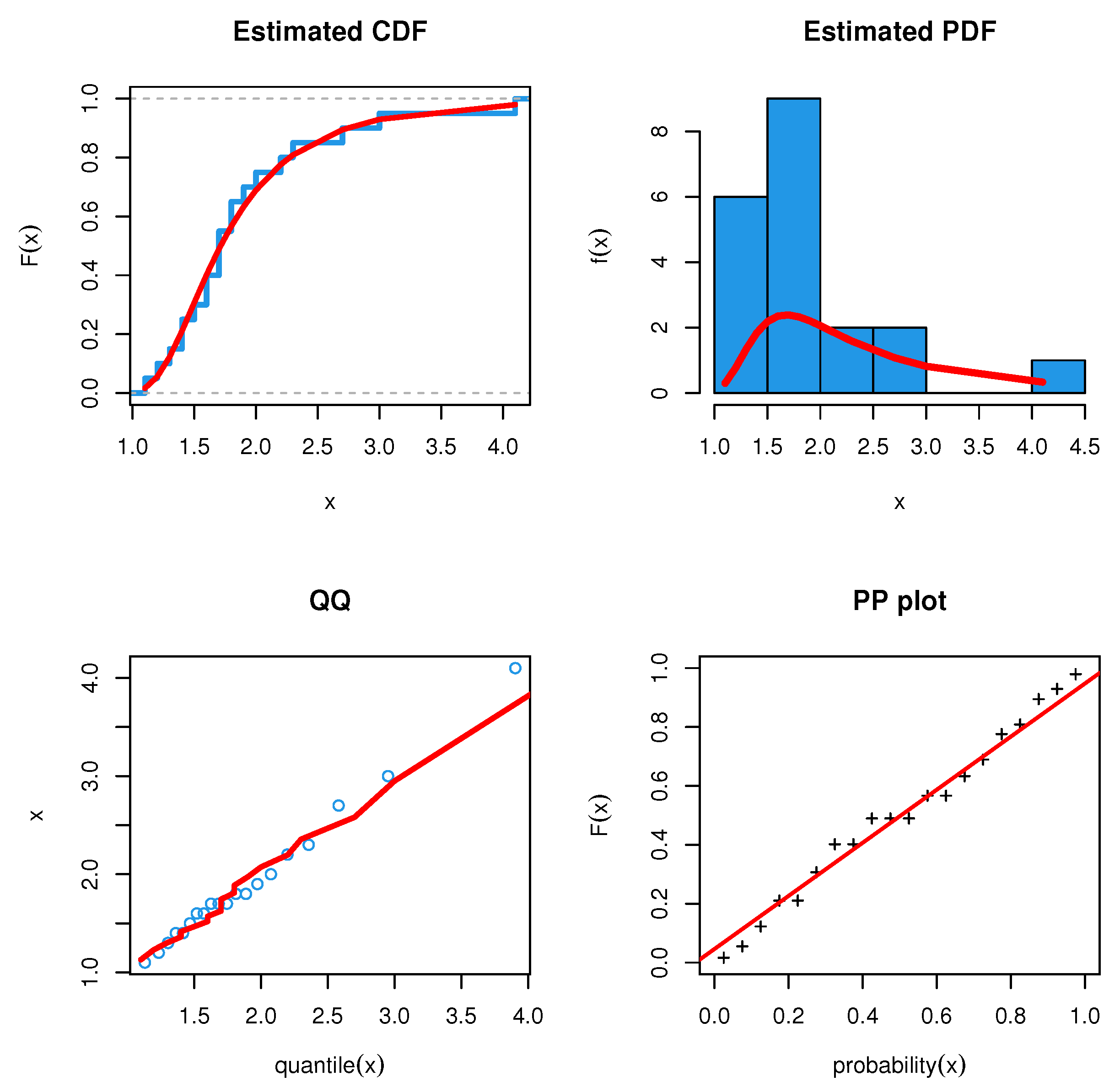
Dataset III: In a third application, we examine the actual patient relief times of twenty patients receiving an analgesic. Ref. [42] examined this data collection. The information is as follows: 1.1, 1.4, 1.3, 1.7, 1.9, 1.8, 1.6, 2.2, 1.7, 2.7, 4.1, 1.8, 1.5, 1.2, 1.4, 3.0, 1.7, 2.3, 1.6,2.0.

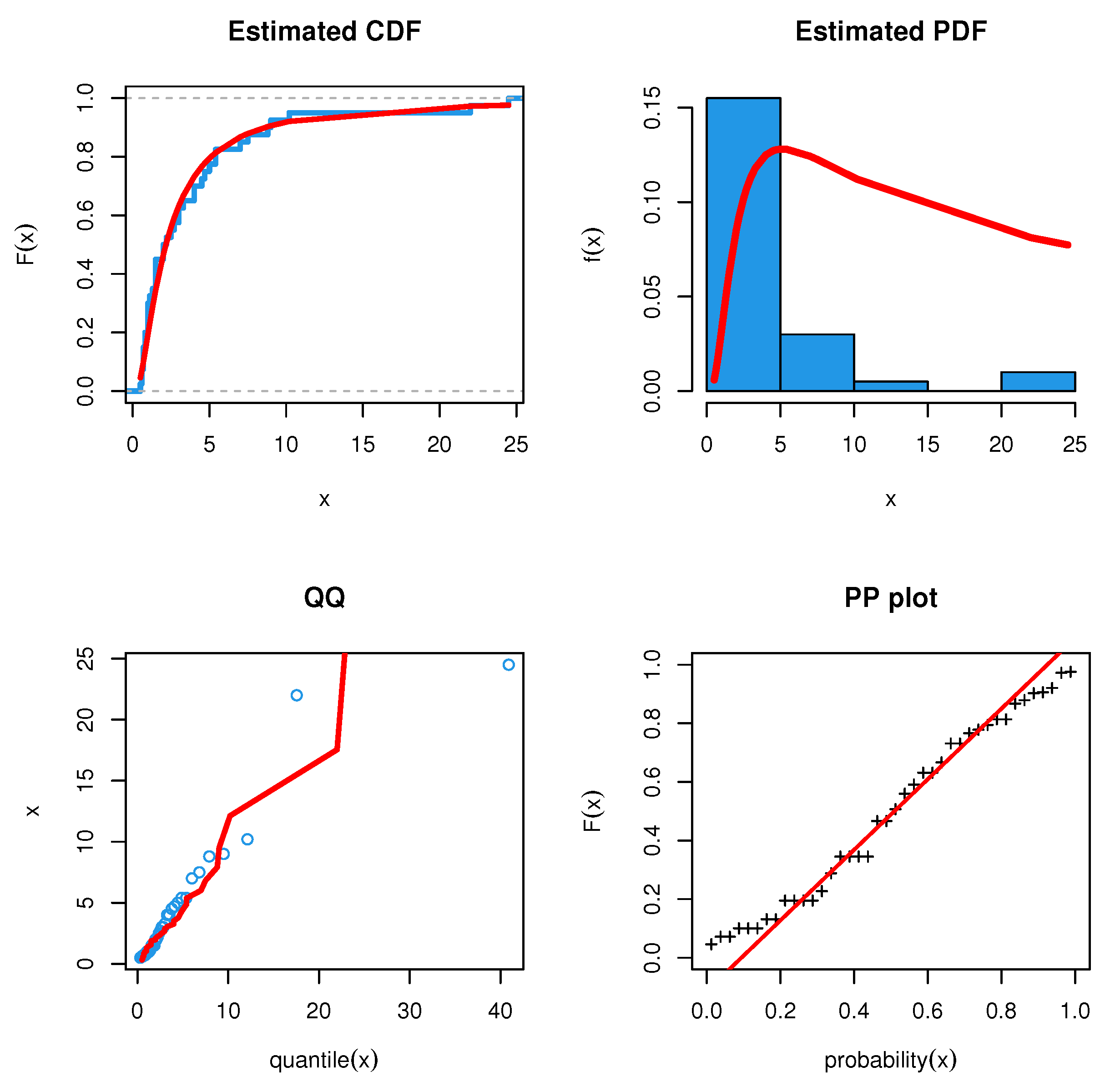
The MLE (corresponding standard errors (SEs)) of the parameters, some measure criteria, and various GF statistical tests of all the models are listed in Table 13, Table 14 and Table 15, respectively, for the two datasets. For both datasets, Figure 11, Figure 12 and Figure 13 present various plots, including the pdf, cdf, PP and QQ along of the FB model.

Table 13. MLE with SE and GF measures with different criteria for first set of data.

		Estimates	SE	KSD	PVKS	AIMC	BIMC	CAIMC	HQIMC	CVMGF	ADGF
	$\lambda$	0.5355	0.2329
FB	p	0.1633	0.1445	0.1048	0.7721	50.7963	55.8629	51.4629	52.6282	0.0691	0.4510
	$\beta$	9.8679	4.4608
	$\beta$	20.1258	36.1195
OPE	$\theta$	30.5538	22.2598	0.1538	0.3004	198.3171	203.3837	198.9837	200.1490	0.1634	1.1722
	$\lambda$	0.0079	0.0054
	$\alpha$	0.1033	0.1125
PL	$\beta$	7.4205	6.9984	0.1290	0.5189	187.1752	192.2418	187.8419	189.0071	0.1090	0.6652
	$\theta$	0.0395	0.1843
	$\alpha$	19.9852	35.6569
Exp-W	$\beta$	0.3292	0.0832	0.1178	0.6356	186.8025	191.8691	187.4691	188.6344	0.0764	0.4648
	$\theta$	23.0309	22.5195
	$\alpha$	0.9607	0.1078
Ext-W	$\beta$	223103.1171	246.9642	0.1289	0.5196	197.0232	202.0899	197.6899	198.8552	0.1456	1.0485
	$\theta$	0.1655	0.1877
	$\alpha$	1.3174	0.1576
OWITL	$\beta$	101.1058	176.3670	0.1164	0.6506	187.8920	192.9587	188.5587	189.7240	0.0714	0.4935
	$\theta$	0.0337	0.0420
	$\alpha$	46.1504	53.9881
APL	$\beta$	1.7805	0.5176	0.1098	0.7684	190.5008	195.5675	191.1675	192.3328	0.0856	0.5773
	$\theta$	1.3384	0.8585
	$\alpha$	2.2755	0.8929
MOL	$\beta$	5.9211	7.0710	0.1172	0.6419	193.2875	198.3541	193.9541	195.1194	0.1088	0.7351
	$\theta$	1.7222	2.2200
	$\alpha$	0.3098	0.4382
EGLBE	$\beta$	0.0791	0.1130	0.1532	0.3049	194.8543	199.9210	195.5210	196.6863	0.1291	0.9493
	$\theta$	0.7923	0.2561

Table 14. MLE with SE and GF measures with different criteria for second set of data.

		Estimates	SE	KSD	PVKS	AIMC	BIMC	CAIMC	HQIMC	CVMGF	ADGF
	$\lambda$	2.2371	0.3112
FB	p	2.5116$\times {10}^{-8}$	0.0575	0.0690	0.9414	383.1894	389.1268	383.3305	385.3271	0.0349	0.2578
	$\beta$	9.1432	2.4928
	$\beta$	0.1403	0.0721
OPE	$\theta$	22.1418	11.2505	0.1356	0.2278	405.7062	411.9388	406.1426	408.1392	0.3502	2.1705
	$\lambda$	0.0078	0.0033
	$\alpha$	0.1403	0.0721
Plomax	$\beta$	22.1418	11.2505	0.1356	0.2278	405.7062	411.9388	406.1426	408.1392	0.3502	2.1705
	$\theta$	0.0078	0.0033
	$\alpha$	69.1436	32.3847
APIW	$\beta$	2.6075	0.2009	0.0702	0.9334	383.2308	389.4634	383.6671	385.6637	0.0443	0.2706
	$\theta$	90.3558	12.3689
	$\alpha$	1.3435	1.6277
Exp-W	$\beta$	0.5320	0.1399	0.0779	0.8665	383.5455	389.7781	383.9818	385.9784	0.0719	0.4149
	$\theta$	49.5045	56.5074
	$\alpha$	1.8426	0.1750
Ext-W	$\beta$	3412.3073	351.4565	0.1433	0.1774	400.5826	406.8152	401.0190	403.0156	0.2924	1.8658
	$\theta$	6.2220	5.5972
	$\alpha$	3.8025	0.3668
OWITL	$\beta$	104.2949	178.5123	0.1235	0.3295	392.1153	398.3479	392.5517	394.5483	0.1886	1.1722
	$\theta$	0.1234	0.0443
	$\alpha$	566.8168	486.4380
APL	$\beta$	13.3274	12.5477	0.0940	0.6744	391.0482	397.2808	391.4846	393.4812	0.1609	0.9583
	$\theta$	64.3030	68.3282
	$\alpha$	3.7693	0.5404
MOL	$\beta$	1637.9293	228.9601	0.0781	0.8641	389.4346	395.6672	389.8710	391.8675	0.1379	0.7799
	$\theta$	1.8279	0.9764
	$\alpha$	0.3233	0.6764
EGLBE	$\beta$	0.0580	0.1226	0.1153	0.4131	388.2659	394.4985	388.7023	390.6989	0.1426	0.8611
	$\theta$	4.4649	1.7588

Table 15. MLE with SE and GF measures with different criteria for third set of data.

		Estimates	SE	KSD	PVKS	AIMC	BIMC	CAIMC	HQIMC	CVMGF	ADGF
	$\lambda$	4.0177	1.3797
FB	p	3.7261$\times {10}^{-7}$	0.2210	0.1019	0.9855	22.3275	25.3147	23.8275	22.9106	0.0287	0.1630
	$\beta$	1.5635	0.3900
	$\beta$	0.0112	0.0103
OPE	$\theta$	30.3292	22.1177	0.1524	0.7420	45.4118	48.3989	46.9118	45.9949	0.1562	0.9134
	$\lambda$	0.0769	0.0482
	$\alpha$	0.0112	0.0103
Plomax	$\beta$	30.3292	22.1177	0.1524	0.7420	45.4118	48.3989	46.9118	45.9949	0.1562	0.9134
	$\theta$	0.0769	0.0482
	$\alpha$	2.6307	2.1605
Exp-W	$\beta$	0.9173	0.2989	0.1351	0.8588	38.3460	41.3332	39.8460	38.9291	0.0532	0.3117
	$\theta$	42.3618	54.2220
	$\alpha$	2.7868	0.4270
Ext-W	$\beta$	142.2474	226.1250	0.1849	0.5008	47.1729	50.1601	48.6729	47.7561	0.1857	1.0928
	$\theta$	854.9621	238.9914
	$\alpha$	2.9900	0.4577
OWITL	$\beta$	335.3102	934.7119	0.1712	0.6011	44.3300	47.3172	45.8300	44.9131	0.1404	0.8302
	$\theta$	0.2191	0.1753
	$\alpha$	806.8877	576.3756
APL	$\beta$	212.7172	52.4565	0.2261	0.2583	47.8483	50.8355	49.3483	48.4315	0.0945	0.5599
	$\theta$	154.6866	38.1556
	$\alpha$	15164.1578	466.2430
MOL	$\beta$	175.1013	183.6170	0.1430	0.8081	44.2687	47.2559	45.7687	44.8518	0.1359	0.7983
	$\theta$	5249.3169	153.8835
	$\alpha$	0.0476	0.0817
EGLBE	$\beta$	0.1075	0.1900	0.1364	0.8510	38.5741	41.5613	40.0741	39.1572	0.0556	0.3267
	$\theta$	25.8842	18.6378

Figure 11. Estimated pdf, estimated cdf, PP and QQ plots for FB distribution for first dataset.

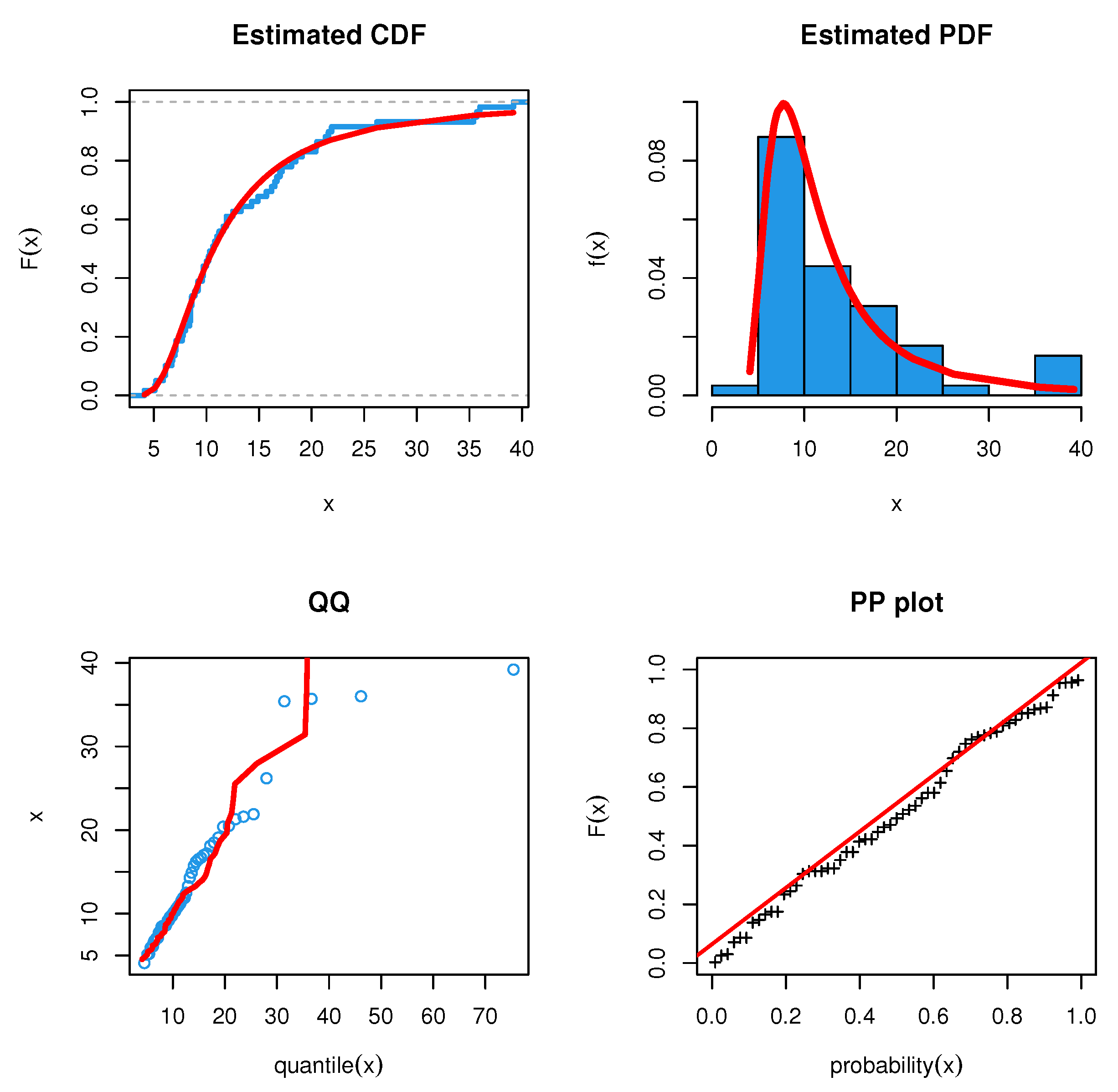
Figure 12. Estimated pdf, estimated cdf, PP and QQ plots for FB distribution for second dataset.

Figure 13. Estimated pdf, estimated cdf, PP and QQ plots for FB distribution for third dataset.

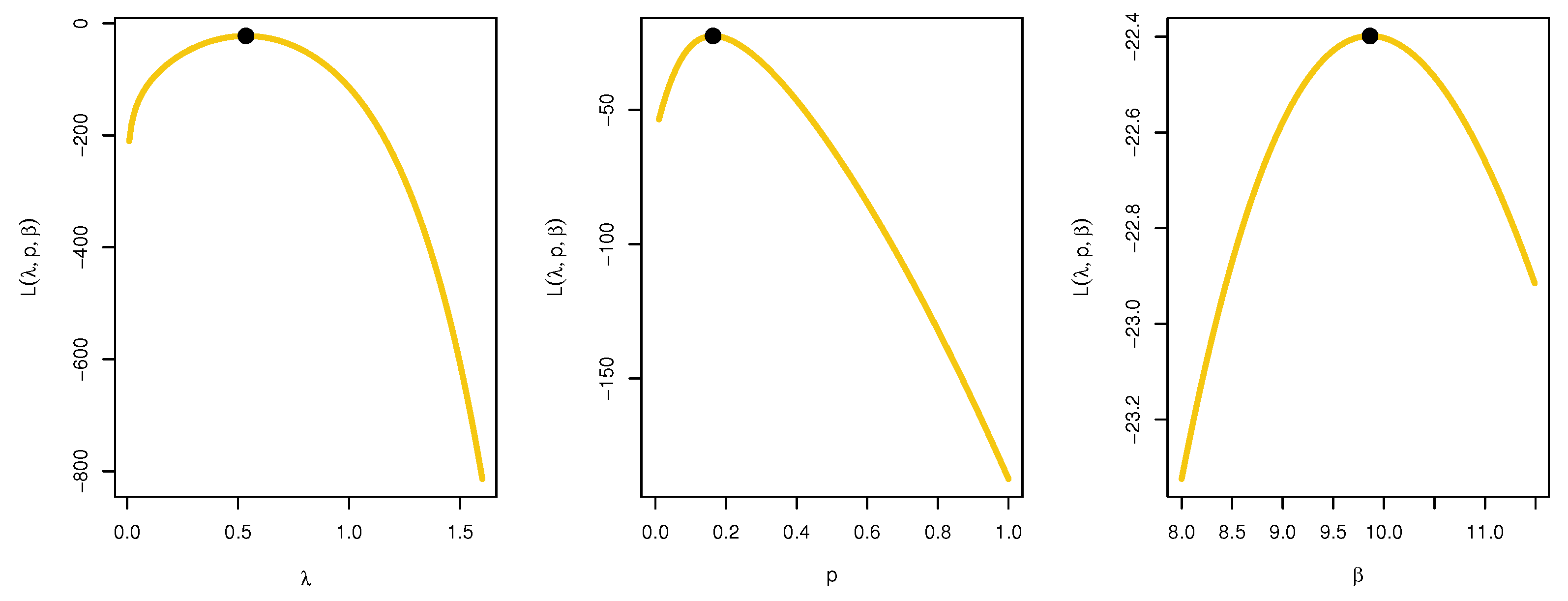
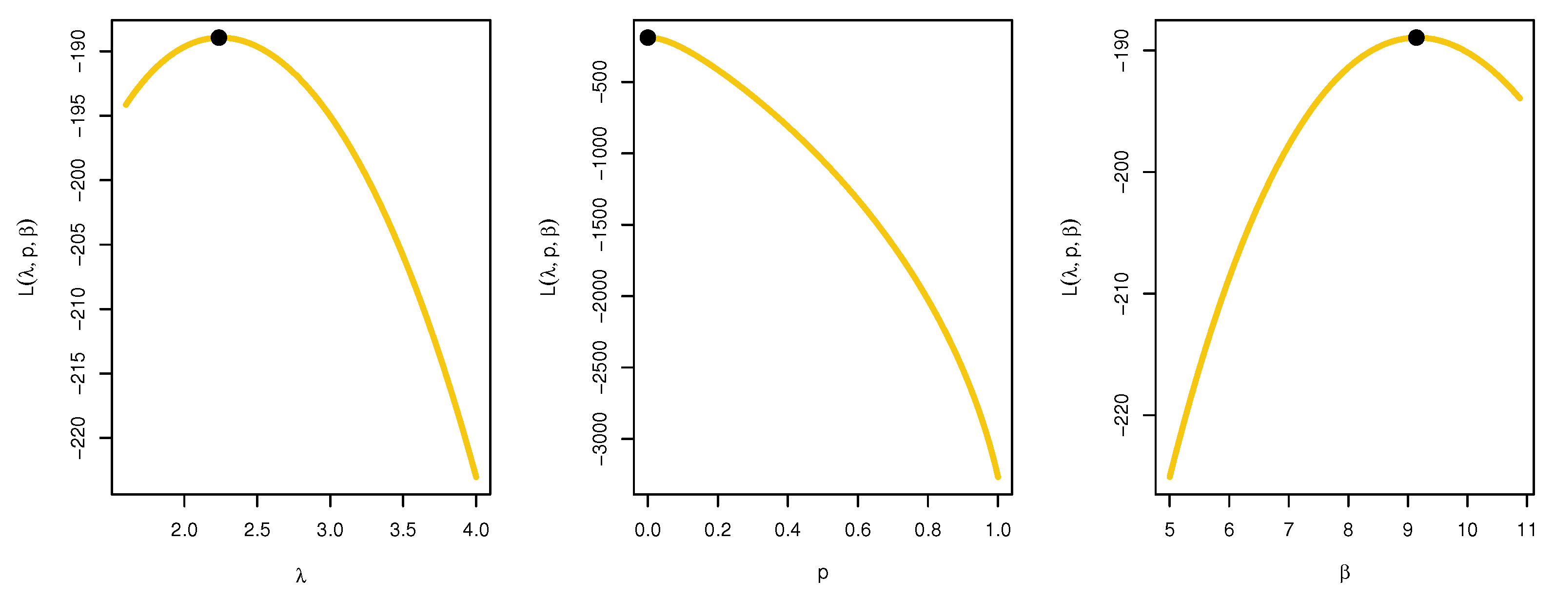
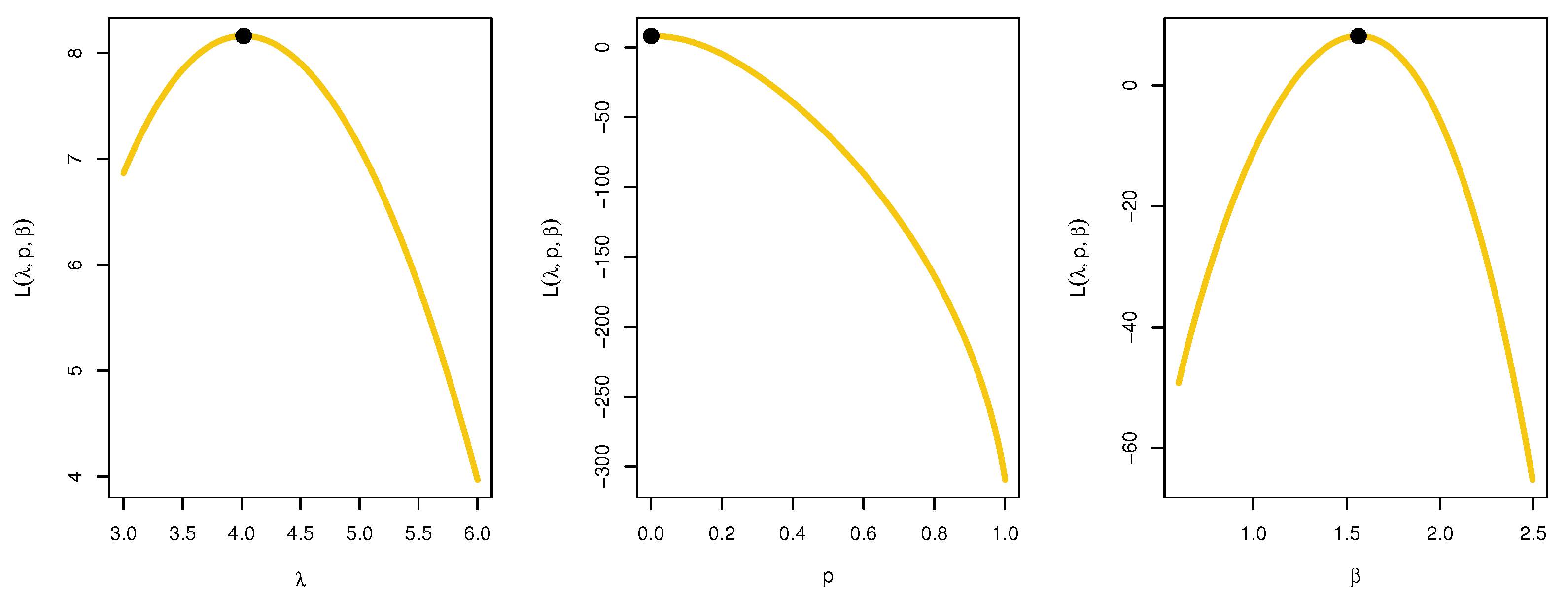
The distribution that has smaller values of key statistics, such as AIMC, BIMC, CAIMC, HQIMC, KSD, CVMGF and ADGF, is generally the one that best fits the data. The findings demonstrate that, compared to the other nine models—namely OPE, PL, APIW, EXP-W, Ext-W, OWITL, APL, MOL and GLBE—the FB distribution offers a significantly superior fit. By fixing one parameter and changing the others, we were able to sketch the log-likelihood for each parameter, as seen in Figure 14, Figure 15, and Figure 16. The graphics demonstrate the excellent behavior of the three datasets since the global maximum values of the three parameter roots can be seen.

Figure 14. Profile likelihood for first dataset.

Figure 15. Profile likelihood for second dataset.

Figure 16. Profile likelihood for third dataset.

8. Conclusions and Summary

In this article, we propose a new lifetime distribution called the Fréchet binomial (FB) distribution. The FB model is very flexible because its pdf can be unimodal, decreasing and right skewness. Furthermore, the hrf can be increasing, decreasing, upside-down and reversed-J form. An important mixture representation of the pdf and cdf were calculated. Different sub-models of the FB model were discussed. Numerous statistical and mathematical features of the FB distribution such as the $Q_{UN}F$, $M_O$, $I{M}_O$, $M_{O}GF$, $PW{M}_O$, order statistics and entropy were calculated. The ACS plans in this article were focused on the FB distribution when the life test was truncated at the desired distribution’s median life. The required sample size was calculated using numerous truncation periods for the different characteristics of the proposed distribution and varying degrees of customer risk. In addition, for the sample sizes acquired, the probability of acceptance was calculated to verify whether it is less than or equal to the complement of the consumer’s risk $(1-p^{*})$. Some relevant tables were supplied that may be used to create ACS plans. Based on the FB distribution, further work may be expanded to provide double and group ACS plans. The estimates of the parameters of the new model were estimated using the ML method. A simulation outcome was conducted to check the performance of the MLE method. Using three real-life datasets, we illustrated the flexibility of the FB model. The new suggested model was compared with eight known statistical models, namely odd Perks exponential (OPE); power Lomax (PL); alpha power inverse Weibull (APIW); exponentiated Weibull (Exp-W); extended Weibull (Ext-W); odd Weibull inverse Topp–Leone (OWITL); alpha power Lomax (APL); Marshall–Olkin Lomax (MOL); and generalization length biased exponential (GLBE) distributions. The new suggested model offers a significantly superior fit.

References

- Fréchet, M. Sur la loi des erreurs dobservation. Bull. Soc. Math. Moscou 1924, 33, 5–8. [Google Scholar]
- Kotz, S.; Nadarajah, S. Extreme Value Distributions: Theory and Applications; Imperial College Press: London, UK, 2000. [Google Scholar]
- Nadarajah, S.; Kotz, S. The exponentiated Fréchet distribution. Inter. Stat. Electron. J. 2003, 14, 1–7. [Google Scholar]
- Nadarajah, S.; Gupta, A.K. The beta Fréchet distribution. Far East J. Theor. Stat. 2004, 14, 15–22. [Google Scholar]
- Mahmoud, M.R.; Mandouh, R.M. On the transmuted Fréchet distribution. J. Appl. Sci. Res. 2013, 9, 5553–5561. [Google Scholar]
- Krishna, E.; Jose, K.; Alice, T.; Ristic, M. The Marshall–Olkin Fréchet distribution. Commun. Stat. Theory Methods 2013, 42, 4091–4107. [Google Scholar] [CrossRef]
- Alotaibi, R.; Almetwally, E.M.; Ghosh, I.; Rezk, H. Classical and Bayesian Inference on Finite Mixture of Exponentiated Kumaraswamy Gompertz and Exponentiated Kumaraswamy Fréchet Distributions under Progressive Type II Censoring with Applications. Mathematics 2022, 10, 1496. [Google Scholar] [CrossRef]
- Elbatal, I.; Asha, G.; Raja, V. Transmuted exponentiated Fréchet distribution: Properties and applications. J. Stat. Appl. Probab. 2014, 3, 379–394. [Google Scholar]
- Mead, M.; Afify, A.Z.; Hamedani, G.G.; Ghosh, I. The beta exponential Fréchet distribution with applications. Austrian J. Stat. 2016, 46, 41–63. [Google Scholar] [CrossRef]
- Mead, M. A note on Kumaraswamy Fréchet distribution. Australia 2014, 8, 294–300. [Google Scholar]
- Abouelmagd, T.H.M.; Hamed, M.S.; Afify, A.Z.; Al-Mofleh, H.; Iqbal, Z. The burr x Fréchet distribution with its properties and applications. Appl. Probab. Stat. 2018, 13, 23–51. [Google Scholar]
- Almetwally, E.M.; Muhammed, H.Z. On a bivariate Fréchet distribution. J. Stat. Appl. Probab. 2020, 9, 1–21. [Google Scholar]
- Alzeley, O.; Almetwally, E.M.; Gemeay, A.M.; Alshanbari, H.M.; Hafez, E.H.; Abu-Moussa, M.H. Statistical inference under censored data for the new exponential-X Fréchet distribution: Simulation and application to leukemia data. Comput. Intell. Neurosci. 2021, 2021, 2167670. [Google Scholar] [CrossRef] [PubMed]
- Afify, A.Z.; Yousof, H.M.; Cordeiro, G.M.; Ortega, E.M.M.; Nofal, Z.M. The Weibull Fréchet distribution and its applications. J. Appl. Stat. 2016, 43, 2608–2626. [Google Scholar] [CrossRef]
- Afify, A.Z.; Yousof, H.M.; Cordeiro, G.M.; Ahmad, M. The Kumaraswamy Marshall-Olkin Fréchet distribution: Properties and Applications. J. ISOSS 2016, 2, 41–58. [Google Scholar]
- Korkmaz, M.C.; Yousof, H.M.; Ali, M.M. Some theoretical and computational aspects of the odd Lindley Fréchet distribution. J. Stat. Stat. Actuar. Sci. 2017, 2, 129–140. [Google Scholar]
- Nasiru, S.; Mwita, P.; Ngesa, O. Alpha power transformed Fréchet distribution. Appl. Math. Inf. Sci. 2019, 13, 129–141. [Google Scholar] [CrossRef]
- Eghwerido, J. The alpha power Weibull Fréchet distribution: Properties and applications. Turk. J. Sci. 2020, 5, 170–185. [Google Scholar]
- Hassan, A.S.; Elgarhy, M.; Nassr, S.G.; Ahmad, Z.; Alrajhi, S. Truncated Weibull Fréchet Distribution: Statistical Inference and Applications. J. Comput. Theor. Nanosci. 2019, 16, 1–9. [Google Scholar] [CrossRef]
- Haq, A.; Elgarhy, M. The odd Fréchet-G class of probability distributions. J. Stat. Appl. Probab. 2018, 7, 189–203. [Google Scholar] [CrossRef]
- Badr, M.; Elbatal, I.; Jamal, F.; Chesneau, C.; Elgarhy, M. The Transmuted Odd Fréchet-G class of Distributions: Theory and Applications. Mathematics 2020, 8, 958. [Google Scholar] [CrossRef]
- Nasiru, S. Extended Odd Fréchet-G class of Distributions. J. Probab. Stat. 2018, 2018, 2931326. [Google Scholar] [CrossRef]
- Jayakumar, K.; Babu, M.G. A new generalization of the Fréchet distribution: Properties and application. Statistica 2019, 79, 267–289. [Google Scholar]
- Baharith, L.; Alamoudi, H. The exponentiated Fréchet Generator of ´ Distributions with Applications. Symmetry 2021, 13, 572. [Google Scholar] [CrossRef]
- Alyami, S.A.; Babu, M.G.; Elbatal, I.; Alotaibi, N.; Elgarhy, M. Type II Half-Logistic Odd Fréchet Class of Distributions: Statistical Theory and Applications. Symmetry 2022, 14, 1222. [Google Scholar] [CrossRef]
- ZeinEldin, R.A.; Chesneau, C.; Jamal, F.; Elgarhy, M.; Almarashi, A.M. and Al-Marzouki, S. Generalized Truncated Fréchet Generated Family Distributions an dTheir Applications. Comput. Model. Eng. Sci. 2021, 126, 791–819. [Google Scholar]
- Al-Marzouki, S.; Jamal, F.; Chesneau, C.; Elgarhy, M. Topp-Leone Odd Fréchet Generated Family of Distributions with Applications to COVID-19 Data Sets. Comput. Model. Eng. Sci. 2020, 125, 437–458. [Google Scholar]
- MacGillivray, H.L. Skewness and asymmetry: Measures and orderings. Ann. Stat. 1986, 14, 994–1011. [Google Scholar] [CrossRef]
- Arnold, B.C.; Balakrishnan, N.; Nagraja, H.N. A First Course in Order Statistics; Society for Industrial and Applied Mathematics: Philadelphia, PA, USA, 2008. [Google Scholar]
- Singh, S.; Tripathi, Y.M. Acceptance sampling plans for inverse Weibull distribution based on truncated life test. Life Cycle Reliab. Saf. Eng. 2017, 6, 169–178. [Google Scholar] [CrossRef]
- Elbatal, I.; Alotaibi, N.; Almetwally, E.M.; Alyami, S.A.; Elgarhy, M. On Odd Perks-G Class of Distributions: Properties, Regression Model, Discretization, Bayesian and Non-Bayesian Estimation, and Applications. Symmetry 2022, 14, 883. [Google Scholar] [CrossRef]
- Rady, E.H.A.; Hassanein, W.A.; Elhaddad, T.A. The power Lomax distribution with an application to bladder cancer data. SpringerPlus 2016, 5, 1–22. [Google Scholar] [CrossRef]
- Basheer, A.M. Alpha power inverse Weibull distribution with reliability application. J. Taibah Univ. Sci. 2019, 13, 423–432. [Google Scholar] [CrossRef]
- Nassar, M.M.; Eissa, F.H. On the exponentiated Weibull distribution. Commun. -Stat.-Theory Methods 2003, 32, 1317–1336. [Google Scholar] [CrossRef]
- Zhang, T.; Xie, M. Failure data analysis with extended Weibull distribution. Commun. Stat. Comput. 2007, 36, 579–592. [Google Scholar] [CrossRef]
- Almetwally, E.M. The odd Weibull inverse topp—leone distribution with applications to COVID-19 data. Ann. Data Sci. 2022, 9, 121–140. [Google Scholar] [CrossRef]
- Almongy, H.M.; Almetwally, E.M.; Mubarak, A.E. Marshall—Olkin alpha power lomax distribution: Estimation methods, applications on physics and economics. Pak. J. Stat. Oper. Res. 2021, 17, 137–153. [Google Scholar] [CrossRef]
- Ghitany, M.E.; Al-Awadhi, F.A.; Alkhalfan, L. Marshall–Olkin extended Lomax distribution and its application to censored data. Commun. Stat. Methods 2007, 36, 1855–1866. [Google Scholar] [CrossRef]
- Maxwell, O.; Oyamakin, S.O.; Chukwu, A.U.; Olusola, Y.O.; Kayode, A.A. New generalization of length biased exponential distribution with applications. J. Adv. Appl. Math. 2019, 4, 82–88. [Google Scholar] [CrossRef]
- Jorgensen, B. Statistical Properties of the Generalized Inverse Gaussian Distribution; Springer: New York, NY, USA, 1982. [Google Scholar]
- Tharshan, R.; Wijekoon, P. Location based generalized Akash distribution: Properties and applications. Open J. Stat. 2020, 10, 163–187. [Google Scholar] [CrossRef]
- Gross, A.J.; Clark, V. Survival Distributions: Reliability Applications in the Biomedical Sciences; John Wiley & Sons: Hoboken, NJ, USA, 1975. [Google Scholar]
Publisher’s Note: MDPI stays neutral with regard to jurisdictional claims in published maps and institutional affiliations. |
© 2022 by the authors. Licensee MDPI, Basel, Switzerland. This article is an open access article distributed under the terms and conditions of the Creative Commons Attribution (CC BY) license (https://creativecommons.org/licenses/by/4.0/).