
A New Discrete Mycorrhiza Optimization Nature-Inspired Algorithm


Abstract
:1. Introduction
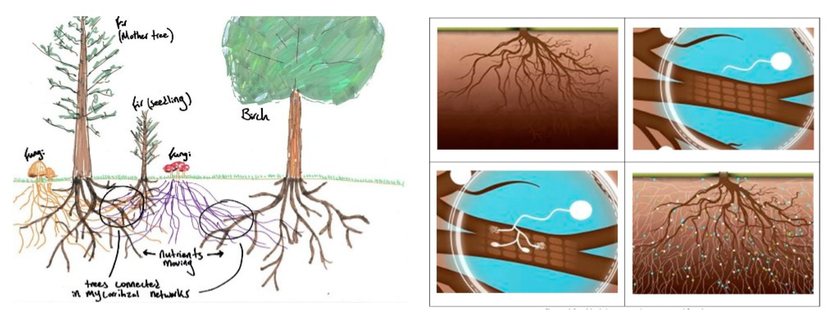
2. Mycorrhiza Network and Plants
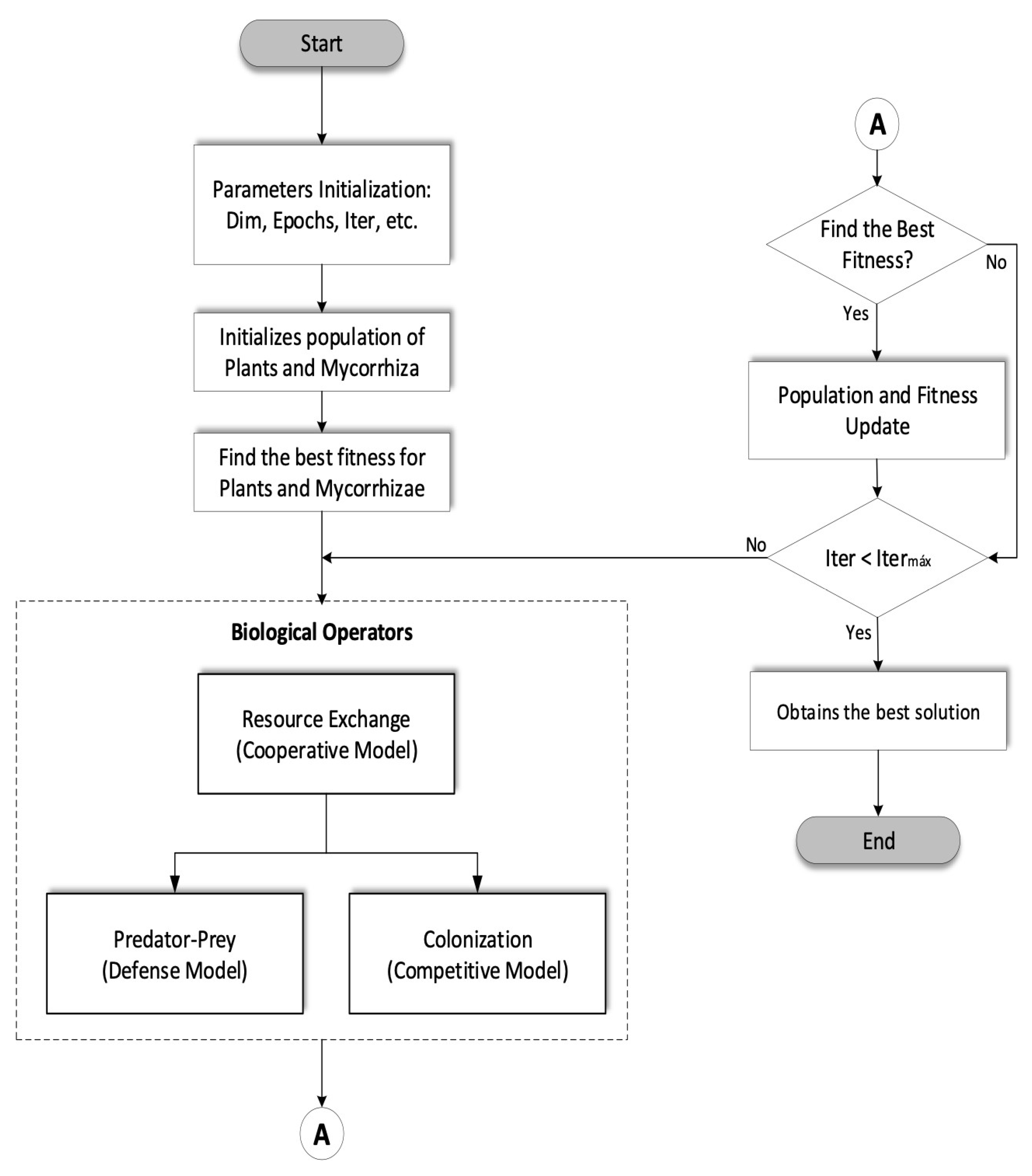
3. Discrete Mycorrhized Optimization Algorithm (DMOA)
- (A)
- Plant defense against external stress and danger situations by means of biochemical signals via the MN.
- (B)
- Cooperation in the ecosystem with the exchange of resources (carbon, water, nitrogen, phosphorus, and other nutrients) through the MN.
- (C)
- Predator-Prey Defense Model: Defensive behavior against predators that can be insects or animals, for the survival of the entire habitat (plants and fungi).
- Resource Exchange Cooperative Model: Exchange of resources, such as carbon, water, nitrogen, phosphorus, and other nutrients to other plants and the fungal network through the MN.
- Colonization Competitive Model: In any ecosystem, resources are limited and all living beings compete to obtain them. In a forest, colonization occurs by the MN, where the different plants and fungi compete for the resources provided by all the members connected by the Mycorrhiza.
3.1. DMOA Pseudocode
| Algorithm 1. Discrete Mycorrhiza Optimization Algorithm (DMOA). |
| Objective min or max f(x), × = (x1, x2, ..., xd) Define parameters (a, b, c, d, e, f, x, y) Initialize a population of n plants and mycorrhiza with random solutions Find the best solution fit in the initial population while (t < maxIter) for i = 1:n (for n plants and Micorrhiza population) end for Apply (LV-Cooperative Model) if else end if rand ([1 2]) if (rand = 1) Apply (LV-Predator-Prey Model) else Apply (LV- Competitive Model) end if Evaluate new solutions. If the new solutions are better, the best new solutions are updated. Find the current best fit solution. end while |
3.2. DMOA Flowchart
3.3. Lotka–Volterra Discrete Equation System
- The six equations are different and each pair of equations corresponding to each biological operator model the conditions under which said operators work.
- The Cooperative model infers randomly in one of the two biological operators of either Defense and Competitive, to try to simulate what can happen in a living and changing ecosystem over time.
3.4. DMOA Parameters
4. Experimental Results
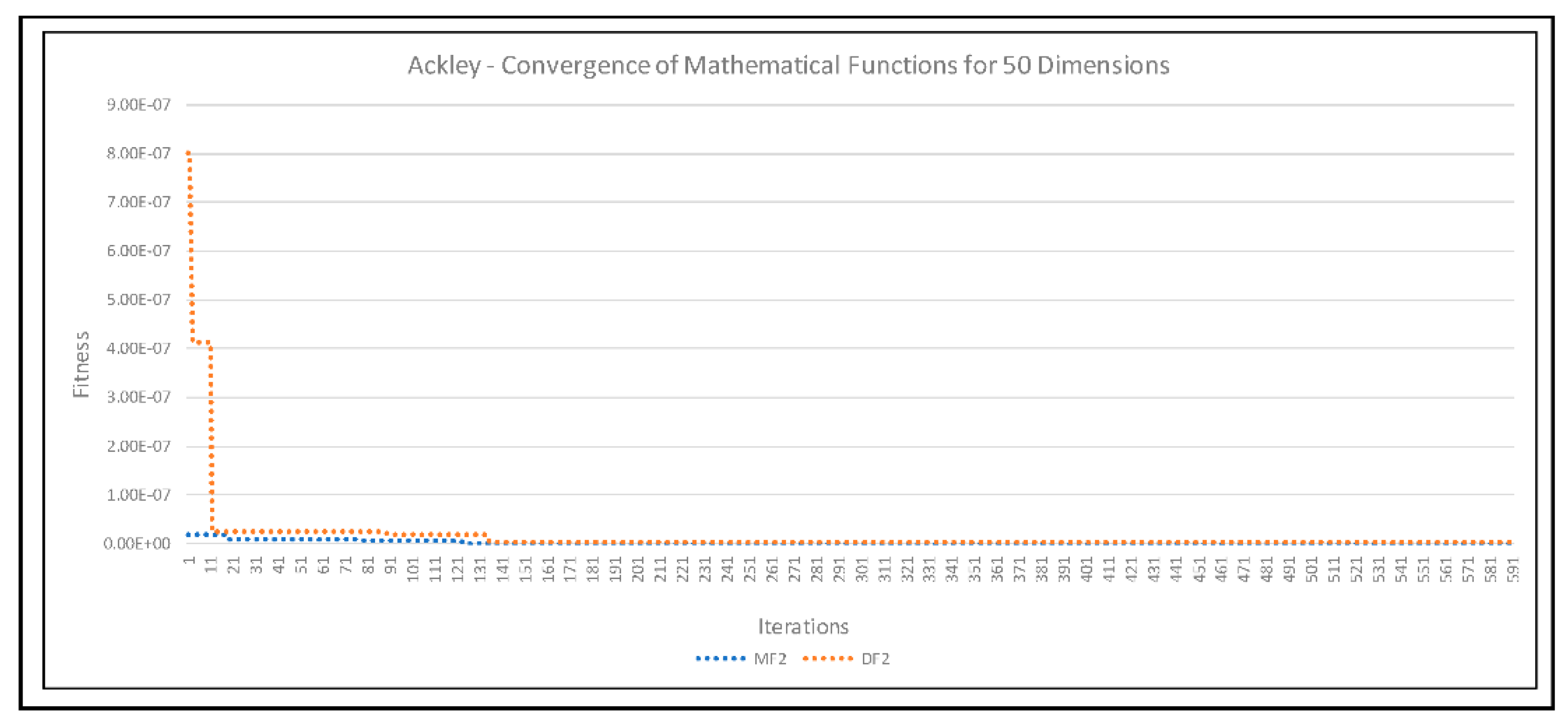
4.1. Results of the MTOA Algorithm Experiments with CEC-2013
4.2. Results of the DMOA Algorithm Experiments with CEC-2013
4.3. Hypothesis Tests
4.4. Compared with Others Methods
4.5. Programming Environment
5. Conclusions
Author Contributions
Funding
Institutional Review Board Statement
Informed Consent Statement
Data Availability Statement
Acknowledgments
Conflicts of Interest
References
- Yang, X.S. Cuckoo Search and Firefly Algorithm: Overview and Analysis. In Cuckoo Search and Firefly Algorithm; Yang, X.-S., Ed.; Springer: Berlin/Heidelberg, Germany, 2014; Volume 516, pp. 1–26. [Google Scholar]
- Malik, H.; Iqbal, A.; Joshi, P.; Agrawal, S.; Bakhsh, F. Metaheuristic and Evolutionary Computation: Algorithms and Applications. Stud. Comput. Intell. 2021, 916, 3–33. [Google Scholar]
- Boussaïd, I.; Lepagnot, J.; Siarry, P. A survey on optimization metaheuristics. Inf. Sci. 2013, 237, 82–117. [Google Scholar] [CrossRef]
- Blum, C.; Roli, A. Metaheuristics in Combinatorial Optimization: Overview and Conceptual Comparison. ACM Comput. Surv. 2001, 35, 268–308. [Google Scholar] [CrossRef]
- Liu, X. A note on the existence of periodic solution in discrete predator-prey models. Appl. Math. Model. 2010, 34, 2477–2483. [Google Scholar] [CrossRef]
- Ghasemabadi, A.; Rahmani, D.; Mohammad, H. Investigating the dynamics of Lotka–Volterra model with disease in the prey and predator species. Int. J. Nonlinear Anal. Appl. IJNAA 2021, 12, 633–648. [Google Scholar]
- O’dwyer, J. Whence Lotka–Volterra? Conservation Laws and Integrable Systems in Ecology. Theor. Ecol. 2018, 11, 441–452. [Google Scholar] [CrossRef]
- Vaidyanathan, S. Lotka–Volterra Two-Species Mutualistic Biology Models and Their Ecological Monitoring. Int. J. Pharm. Tech. Res. 2015, 8, 199–212. [Google Scholar]
- Din, Q. Dynamics of a discrete Lotka–Volterra model. Adv. Differ. Equ. 2013, 2013, 95. [Google Scholar] [CrossRef]
- Xu, L.; Zou, L.; Chang, Z.; Lou, S.; Peng, X.; Zhang, G. Bifurcation in a Discrete Competition System. Discret. Dyn. Nat. Soc. 2014, 2014, 193143. [Google Scholar] [CrossRef]
- Xu, L.; Lou, S.; Xu, P.; Zhang, G. Feedback Control and Parameter Invasion for a Discrete Competitive Lotka–Volterra System. Discret. Dyn. Nat. Soc. 2018, 2018, 7473208. [Google Scholar] [CrossRef] [Green Version]
- Lotka, A.J. Element of Physical Biology. Sci. Prog. Twent. Century 1919, 21, 341–343. [Google Scholar]
- Volterra, V. Variations and Fluctuations of the Number of Individuals in Animal Species living together. ICES J. Mar. Sci. 1928, 3, 3–51. [Google Scholar] [CrossRef]
- Carreon-Ortiz, H.; Valdez, F.; Castillo, O. A new mycorrhized tree optimization nature-inspired algorithm. Soft Comput. 2022, 26, 4797–4817. [Google Scholar] [CrossRef]
- Teste, F.; Simard, S.; Durall, D.; Guy, R.; Jones, M.; Schoonmaker, A. Access to mycorrhizal networks and roots of trees: Importance for seedling survival and resource transfer. Ecology 2009, 90, 2808–2822. [Google Scholar] [CrossRef] [PubMed]
- Simard, S.W. (Ed.) Memory and Learning in Plants. In Signaling and Communication in Plants; Springer: Cham, Switzerland, 2018; pp. 191–213. [Google Scholar]
- Molina, R.; Massicotte, H.; Trappe, J.M. Specificity phenomenon in mycorrhizal symbiosis: Community-ecological consequences and practical implications. In Mycorrhizal Functioning: An Integrative Plant-Fungal Process; Allen, M., Ed.; Chapman Hall: London, UK, 1992; pp. 357–423. [Google Scholar]
- Simard, S.W.; Perry, D.A.; Jones, M.D. Net transfer of carbon between ectomycorrhizal tree species in the field. Nature 1997, 388, 579–582. [Google Scholar] [CrossRef]
- Birch, J.; Simard, S.W.; Beiler, K.; Karst, J. Beyond seedlings: Ectomycorrhizal fungal networks and growth of mature Pseudotsuga menziesii. J. Ecol. 2020, 109, 808–818. [Google Scholar] [CrossRef]
- He, X.H.; Bledsoe, C.S.; Zasoski, R.J. Rapid nitrogen transfer from ectomycorrhizal pines to adjacent ectomycorrhizal and arbuscular mycorrhizal plants in a California oak woodland. New Phytol. 2006, 170, 143–151. [Google Scholar] [CrossRef]
- Nara, K. Ectomycorrhizal networks and seedling establishment during early primary succession. New Phytol. 2006, 169, 169–178. [Google Scholar] [CrossRef]
- Egerton-Warburton, L.M.; Querejeta, J.I.; Allen, M.F. Common mycorrhizal networks provide a potential pathway for the transfer of hydraulically lifted water between plants. J. Exp. Bot. 2007, 58, 1473–1483. [Google Scholar] [CrossRef]
- Warren, J.M.; Brooks, R.; Meinzer, F.C. Hydraulic redistribution of water from Pinus ponderosa trees to seedlings: Evidence for an ectomycorrhizal pathway. New Phytol. 2008, 178, 382–394. [Google Scholar] [CrossRef]
- Song, Y.; Simard, S.; Carroll, A.; Mohn, W.W.; Zeng, R.S. Defoliation of interior Douglas-fir elicits carbon transfer and stress signalling to ponderosa pine neighbors through ectomycorrhizal networks. Sci. Rep. 2015, 5, 8495. [Google Scholar] [CrossRef] [PubMed] [Green Version]
- Kytoviita, M.M.; Vestberg, M.; Tuomi, J. A test of mutual aid in common mycorrhizal networks: Established vegetation negates benefit in seedlings. Ecology 2003, 84, 898–906. [Google Scholar] [CrossRef]
- Nara, K.; Hogetsu, T. Ectomycorrhizal fungi on established shrubs facilitate subsequent seedling establishment of successional plant species. Ecology 2004, 85, 1700–1707. [Google Scholar] [CrossRef]
- Simard, S.W.; Durall, D.M. Mycorrhizal networks: A review of their extent, function, and importance. Can. J. Bot. 2004, 82, 1140–1165. [Google Scholar] [CrossRef]
- Cline, E.T.; Ammirati, J.F.; Edmonds, R.L. Does proximity to mature trees influence ectomycorrhizal fungus communities of Douglas-fir seedlings. New Phytol. 2005, 166, 993–1009. [Google Scholar] [CrossRef]
- Mcguire, K.L. Common ectomycorrhizal networks may maintain monodominance in a tropical rain forest. Ecology 2007, 8, 567–574. [Google Scholar] [CrossRef]
- Myers, J.A.; Kitajima, K. Carbohydrate storage enhances seedling shade and stress tolerance in a neotropical forest. J. Ecol. 2007, 95, 383–395. [Google Scholar] [CrossRef]
- Simard, S.W. Mycorrhizal Networks and Seedling Establishment in Douglas-Fir Forests. In Biocomplexity of Plant-Fungal Interactions; Wiley-Blackwell: West Sussex, UK, 2012; pp. 85–107. [Google Scholar]
- Teste, F.P.; Simard, S.W.; Durall, D.M. Role of mycorrhizal networks and tree proximity in ectomycorrhizal colonization of planted seedlings. Fungal Ecol. 2009, 2, 21–30. [Google Scholar] [CrossRef]
- Defrenne, C.E.; Philpott, T.J.; Guichon, S.H.A.; Roach, W.J.; Pickles, B.J.; Simard, S.W. Shifts in Ectomycorrhizal Fungal Communities and and Exploration Types Relate to the Environment and Fine-Root Traits Across Interior Douglas-Fir Forests of Western Canada. Front. Plant Sci. 2019, 10, 643. [Google Scholar] [CrossRef] [Green Version]
- Barker, J.S.; Simard, S.W.; Jones, M.D.; Durall, D.M. Ectomycorrhizal fungal community assembly on regenerating Douglas-fir after wildfire and clearcut harvesting. Oecologia 2013, 172, 1179–1189. [Google Scholar] [CrossRef]
- Gorzelak, M.; Asay, A.; Pickles, B.; Simard, S.W. Inter-plant communication through mycorrhizal networks mediates complex adaptive behaviour in plant communities. AoB Plants 2015, 7, plv050. [Google Scholar] [CrossRef] [Green Version]
- Lin, L.; Yi, L.; Chaoling, L. Dynamics for a discrete competition and cooperation model of two enterprises with multiple delays and feedback controls. Open Math. 2017, 15, 218–232. [Google Scholar]
- Zhao, M.; Xuan, Z.; Li, C. Dynamics of a discrete-time predator-prey system. Adv. Differ. Equ. 2016, 2016, 191. [Google Scholar] [CrossRef] [Green Version]
- Din, Q.; Khan, M.I. A Discrete-Time Model for Consumer–Resource Interaction with Stability, Bifurcation and Chaos Control. Qual. Theory Dyn. Syst. 2021, 20, 56. [Google Scholar] [CrossRef]
- Zhou, Z.; Zou, X. Stable periodic solutions in a discrete periodic logistic equation. Appl. Math. Lett. 2003, 16, 165–171. [Google Scholar] [CrossRef] [Green Version]
- Krebs, W. A general predator-prey model. Math. Comput. Model. Dyn. Syst. 2003, 9, 387–401. [Google Scholar] [CrossRef]
- Müller, J.; Kuttler, C. Methods and Models in Mathematical Biology, Deterministic and Stochastic Approaches. In Lecture Notes on Mathematical Modelling in the Life Sciences; Springer: Berlin/Heidelberg, Germany, 2015; pp. 157–291. [Google Scholar]
- Brauer, F.; Castillo-Chavez, C. Mathematical Models in Population Biology and Epidemiology, 2nd ed.; Springer: New York, NY, USA; Dordrecht, The Netherlands; Heidelberg, Germany; London, UK, 2012; pp. 123–134. [Google Scholar]
- Chou, C.S.; Friedman, A. Introduction to Mathematical Biology, Modeling, Analysis, and Simulations. In Springer Undergraduate Texts in Mathematics and Technology; Springer International Publishing: Cham, Switzerland, 2016; pp. 51–63. [Google Scholar]
- Radin, M.A. Difference Equations for Scientists and Engineering, Interdisciplinary Difference Equations; World Scientific Publishing: Singapore, 2019; pp. 77–145. [Google Scholar]
- Camouzis, E.; Ladas, G. Dynamics of Third-Order Rational Difference Equations with Open Problems and Conjectures; Chapman & Hall/CRC Press: Boca Raton, FL, USA, 2008. [Google Scholar]
- Elaydi, S. An Introduction to Difference Equations (Undergraduate Texts in Mathematics); Springer: New York, NY, USA, 2005. [Google Scholar]
- Agarwal, R.P.; Wong, P. Advanced Topics in Difference Equations; Springer Science+Business MediaL: Dordrecht, The Netherlands, 1997. [Google Scholar]
- Elaydi, S.; Hamaya, Y.; Matsunaga, H.; Pötzsche, C. Advances in Difference Equations and Discrete Dynamical Systems; Springer Proceedings in Mathematics & Statistics; Springer Nature Singapore Pte Ltd.: Singapore, 2017; pp. 125–135. [Google Scholar]
- Grove, E.A.; Ladas, G. Periodicities in Nonlinear Difference Equations; Chapman & Hall/CRC Press: Boca Raton, FL, USA, 2005. [Google Scholar]
- Aloqeili, M. Dynamics of a rational difference equation. Appl. Math. Comput. 2006, 176, 768–776. [Google Scholar] [CrossRef]
- Mickens, R.E. A note on exact finite difference schemes for modified Lotka–Volterra differential equations. J. Differ. Equ. Appl. 2018, 24, 1016–1022. [Google Scholar] [CrossRef]
- Stevic, S. On some solvable systems of difference equations. Appl. Math. Comput. 2012, 218, 5010–5018. [Google Scholar] [CrossRef]
- Bajo, I.; Liz, E. Global behaviour of a second-order nonlinear difference equation. J. Differ. Equ. Appl. 2011, 17, 1471–1486. [Google Scholar] [CrossRef] [Green Version]
- Senada, K.; Kulenović, M.; Pilav, E. Dynamics of a two-dimensional system of rational difference equations of Leslie-Gower type. Adv. Differ. Equ. 2011, 2011, 29. [Google Scholar]
- Touafek, N.; Elsayed, E.M. On the solutions of systems of rational difference equations. Math. Comput. Model. 2012, 55, 1987–1997. [Google Scholar] [CrossRef]
- Touafek, N.; Elsayed, E.M. On the periodicity of some systems of nonlinear difference equations. Bull. Math. Soc. Sci. Math. Roum 2012, 2, 217–224. [Google Scholar]
- Din, Q. On A System of Rational Difference Equation. Demonstr. Math. 2012, 47, 2014–2026. [Google Scholar] [CrossRef]
- Din, Q. Global behavior of a rational difference equation. Acta Univ. Apulensis 2013, 34, 35–49. [Google Scholar]
- Din, Q.; Qureshi, M.; Khan, A. Dynamics of a fourth-order system of rational difference equations. Adv. Differ. Equ. 2012, 2012, 215. [Google Scholar] [CrossRef] [Green Version]
- Zhang, Q.; Yang, L.; Liu, J. Dynamics of a system of rational third-order difference equation. Adv. Differ. Equ. 2012, 2012, 136. [Google Scholar] [CrossRef] [Green Version]
- Shojaei, M.; Saadati, R.; Adibi, H. Stability and periodic character of a rational third order difference equation. Chaos Solitons Fractals 2009, 39, 1203–1209. [Google Scholar] [CrossRef]
- Elsayed, E.M. Behavior and expression of the solutions of some rational difference equations. J. Comput. Anal. Appl. 2013, 15, 73–81. [Google Scholar]
- Saha, P.; Bairagi, N.; Biswas, M. On the Dynamics of a Discrete Predator-Prey Model. In Trends in Biomathematics: Modeling, Optimization and Computational Problems; Mondaini, R., Ed.; Springer: Berlin/Heidelberg, Germany, 2018; pp. 219–232. [Google Scholar]
- Anderson, D.R.; Sweeney, D.J.; Williams, T.A.; Camm, J.D.; Cochran, J.J.; Fry, M.J.; Ohlmann, J.W. Statistics for Business & Economics, 14th ed.; Cengage: Boston, MA, USA, 2020; pp. 483–489. [Google Scholar]
- Triola, M. Elementary Statistics, 13th ed.; Pearson Education Boston: Boston, MA, USA, 2018; pp. 428–442. [Google Scholar]
- Johnson, R.; Kuby, P. Elementary Statistics, 17th ed.; Cengage Boston: Boston, MA, USA, 2012; pp. 498–504. [Google Scholar]
- Larson, R.; Farber, B. Elementary Statistics Picturing the World, 7th ed.; Pearson: London, UK, 2019; pp. 440–449. [Google Scholar]
- Caraveo, C.; Valdez, F.; Castillo, O. A New Bio-Inspired Optimization Algorithm Based on the Self-Defense Mechanism of Plants in Nature; SpringerBriefs in Applied Sciences and Technology Computational Intelligence; Division of Graduate Studies Tijuana Institute of Technology: Tijuana, Mexico, 2019; pp. 23–52. [Google Scholar]
- Rakhshani, H.; Rahati, A. Snap-drift cuckoo search: A novel cuckoo search optimization algorithm. Appl. Soft Comput. 2017, 52, 771–794. [Google Scholar] [CrossRef]
- Tvrdık, J.; Polakova, R. Competitive Differential Evolution Applied to CEC 2013 Problems. In Proceedings of the 2013 IEEE Congress on Evolutionary Computation, Cancún, México, 20–23 June 2013; pp. 1651–1657. [Google Scholar]
- Joyce, T.; Herrmann, J.M. A Review of No Free Lunch Theorems, and Their Implications for Metaheuristic Optimisation. Stud. Comput. Intell. 2018, 744, 27–51. [Google Scholar]
- Djafari-Rouhani, B.; Khatibzadeh, H. Nonlinear Evolution and Difference Equations of Monotone Type in Hilbert Spaces; Taylor & Francis Group, LLC.: Tokyo, Japan, 2019; pp. 129–205. [Google Scholar]


| Model | Discrete Equations |
|---|---|
| Predator-Prey (Defense) | |
| Competitive (Colonization) | |
| Cooperative (Resource Exchange) |
| Description | Parameter | Value |
|---|---|---|
| Population x at time t | ||
| Population x at time t | ||
| Grow rates of populations x at time t | ||
| Grow rates of populations y at time t | ||
| time | t | |
| Population growth rate x | a | 0.01 |
| Influence of population x on itself | b | 0.02 |
| Influence of population y on population x | g | 0.06 |
| Population growth rate y | d | 0 |
| Influence of population x on population y | e | 1.70 |
| Influence of population y on itself | h | 0.09 |
| Initial population in x | x | 0.0002 |
| Initial population in y | y | 0.0006 |
| Population size | Population | 20 |
| Number of populations | Populations | 2 |
| Dimensions size | Dimensions | 30, 50, 100 |
| Number of epochs | Epochs | 30 |
| Iterations size | Iterations | 30, 50, 100, 500 |
| In the absence of population x = 0, In the absence of population y = 0 | ||
| a, b, c, d, e and f—are positive constants | ||
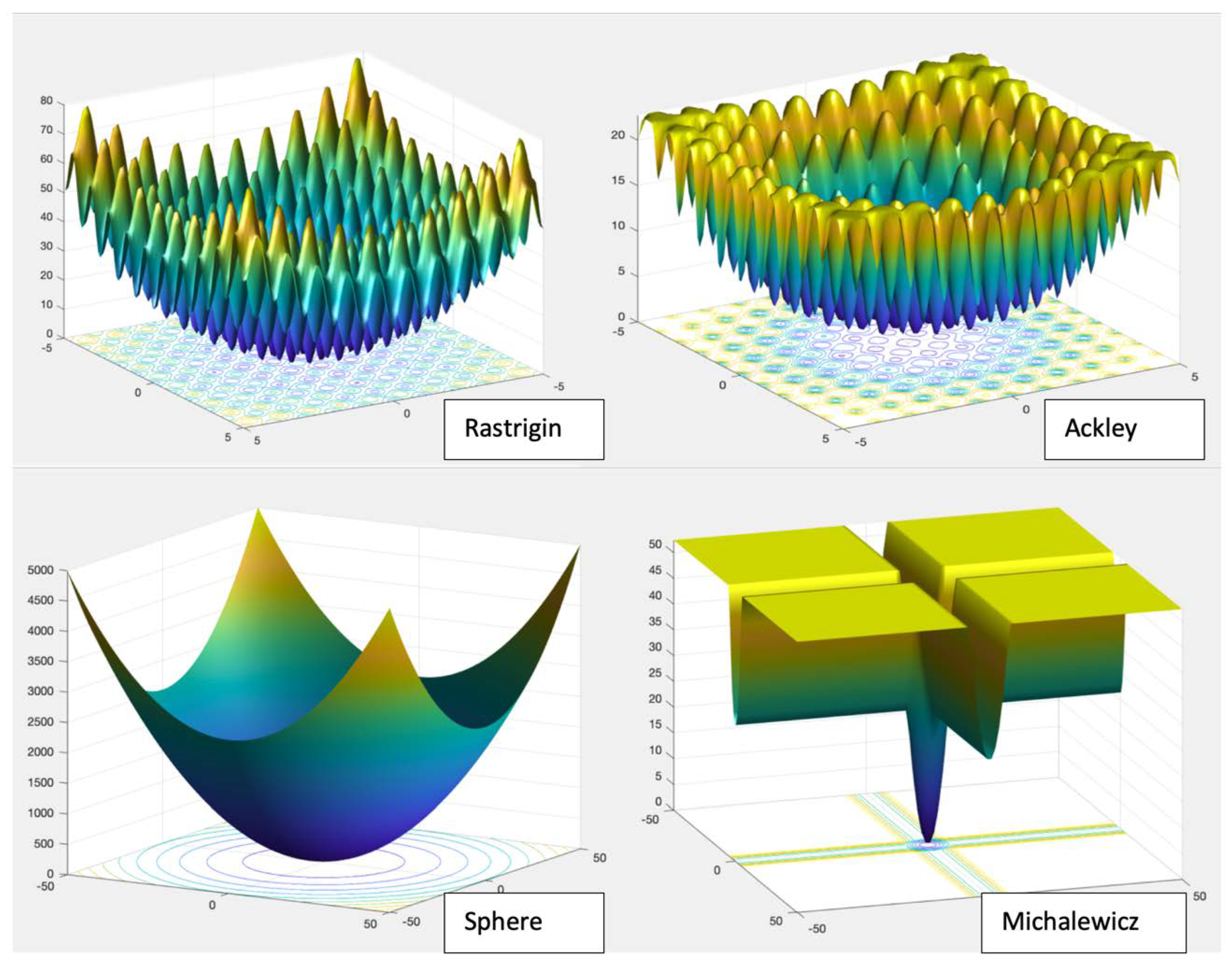
| Fn | Function | Range | Nature |
|---|---|---|---|
| F1 | Sphere | [−5.12, 5.12] | U |
| F2 | Rosenbrok | [42] | U |
| F3 | Griewank | [−600, 600] | M |
| F4 | Rastrigin | [−5.12, 5.12] | M |
| F5 | Ackley | [−32.768, 32.768] | M |
| F6 | Dixon-Price | [42] | U |
| F7 | Michalewicz | [0, π] | M |
| F8 | Powell | [15] | U |
| F9 | RHE—Rotate Hyper Ellipsoid | [−65.536, 65.536] | U |
| F10 | Schwefel | [−500, 500] | M |
| F11 | Styblinski-Tang | [15] | U |
| F12 | SDP—Sum Different Powers | [1] | M |
| F13 | Sum Squares | [42] | U |
| F14 | Trid | [−d2, d2] | U |
| F15 | Zakharov | [42] | U |
| F16 | Bukin No 6 | [−15, −5] | U |
| F17 | Cross-in Tray | [42] | M |
| F18 | Drop-Wave | [−5.12. 5.12] | M |
| F19 | Eggholder | [−5.12, 5.12] | M |
| F20 | Beale | [−4.5, 4.5] | U |
| F21 | Holder-Table | [42] | M |
| F22 | Branin | [42] | M |
| F23 | Levy | [42] | M |
| F24 | Levy 13 | [42] | M |
| F25 | Schaffer 2 | [−100, 100] | M |
| F26 | Schaffer 4 | [−100, 100] | M |
| F27 | Shubert | [42] | M |
| F28 | Bohachevsky 1 | [−100, 100] | M |
| F29 | Bohachevsky 2 | [−100, 100] | M |
| F30 | Bohachevsky 3 | [−100, 100] | M |
| F31 | Booth | [42] | U |
| F32 | Matyas | [42] | U |
| F33 | Mccormick | [−1.5, 4] | U |
| F34 | Easom | [−100, 100] | U |
| F35 | Goldstein-Price | [2] | M |
| F36 | Three-Hump Camel | [15] | M |
| Dim | 30 | |||||||
|---|---|---|---|---|---|---|---|---|
| Iter | 30 | 50 | 100 | 500 | ||||
| Func | Mean | SD | Mean | SD | Mean | SD | Mean | SD |
| f1 | 4.72 × 10⁻⁸ | 1.98 × 10⁻⁸ | 3.28 × 10⁻⁸ | 1.25 × 10⁻⁸ | 2.34 × 10⁻⁸ | 8.91 × 10⁻⁹ | 8.11 × 10⁻⁹ | 4.79 × 10⁻⁹ |
| f2 | 1.67 × 10⁻⁸ | 1.06 × 10⁻⁸ | 8.33 × 10⁻⁹ | 6.77 × 10⁻⁹ | 6.17 × 10⁻¹⁰ | 3.78 × 10⁻¹⁰ | 1.64 × 10⁻⁹ | 1.39 × 10⁻⁹ |
| f3 | 1.29 × 10⁻⁸ | 7.35 × 10⁻⁹ | 4.32 × 10⁻⁹ | 3.38 × 10⁻⁹ | 2.67 × 10⁻¹⁰ | 1.21 × 10⁻¹⁰ | 1.44 × 10⁻⁹ | 1.21 × 10⁻⁹ |
| f4 | 3.85 × 10⁻⁸ | 1.69 × 10⁻⁸ | 2.78 × 10⁻⁸ | 1.16 × 10⁻⁸ | 2.29 × 10⁻⁸ | 1.04 × 10⁻⁸ | 8.13 × 10⁻⁹ | 4.42 × 10⁻⁹ |
| f5 | 5.62 × 10⁻⁸ | 2.45 × 10⁻⁸ | 3.26 × 10⁻⁸ | 1.34 × 10⁻⁸ | 4.30 × 10⁻⁸ | 1.99 × 10⁻⁸ | 6.58 × 10⁻⁹ | 3.32 × 10⁻⁹ |
| f6 | 3.12 × 10⁻⁸ | 1.88 × 10⁻⁸ | 2.63 × 10⁻⁸ | 9.75 × 10⁻⁹ | 2.21 × 10⁻⁸ | 9.88 × 10⁻⁹ | 6.76 × 10⁻⁹ | 4.01 × 10⁻⁹ |
| f7 | 3.51 × 10⁻⁸ | 1.94 × 10⁻⁸ | 2.51 × 10⁻⁸ | 1.12 × 10⁻⁸ | 1.55 × 10⁻⁸ | 7.70 × 10⁻⁹ | 5.70 × 10⁻⁹ | 3.18 × 10⁻⁹ |
| f8 | 4.49 × 10⁻⁸ | 2.02 × 10⁻⁸ | 2.52 × 10⁻⁸ | 1.17 × 10⁻⁸ | 1.98 × 10⁻⁸ | 9.02 × 10⁻⁹ | 9.13 × 10⁻⁹ | 2.87 × 10⁻⁹ |
| f9 | 3.88 × 10⁻⁸ | 1.93 × 10⁻⁸ | 2.27 × 10⁻⁸ | 9.90 × 10⁻⁹ | 1.97 × 10⁻⁸ | 9.81 × 10⁻⁹ | 6.95 × 10⁻⁹ | 3.99 × 10⁻⁹ |
| f10 | 4.95 × 10⁻⁸ | 1.86 × 10⁻⁸ | 2.57 × 10⁻⁸ | 1.37 × 10⁻⁸ | 1.60 × 10⁻⁸ | 9.72 × 10⁻⁹ | 8.42 × 10⁻⁹ | 4.41 × 10⁻⁹ |
| f11 | 3.91 × 10⁻⁸ | 2.31 × 10⁻⁸ | 3.20 × 10⁻⁸ | 1.06 × 10⁻⁸ | 1.98 × 10⁻⁸ | 9.47 × 10⁻⁹ | 8.11 × 10⁻⁹ | 4.14 × 10⁻⁹ |
| f12 | 4.09 × 10⁻⁸ | 2.16 × 10⁻⁸ | 2.26 × 10⁻⁸ | 1.18 × 10⁻⁸ | 2.02 × 10⁻⁸ | 1.09 × 10⁻⁸ | 6.34 × 10⁻⁹ | 3.72 × 10⁻⁹ |
| f13 | 4.03 × 10⁻⁸ | 1.87 × 10⁻⁸ | 2.40 × 10⁻⁸ | 1.20 × 10⁻⁸ | 2.02 × 10⁻⁸ | 9.20 × 10⁻⁹ | 8.02 × 10⁻⁹ | 4.68 × 10⁻⁹ |
| f14 | 4.80 × 10⁻⁸ | 2.22 × 10⁻⁸ | 2.12 × 10⁻⁸ | 1.09 × 10⁻⁸ | 2.24 × 10⁻⁸ | 1.03 × 10⁻⁸ | 7.02 × 10⁻⁹ | 3.78 × 10⁻⁹ |
| f15 | 4.41 × 10⁻⁸ | 2.11 × 10⁻⁸ | 2.21 × 10⁻⁸ | 1.28 × 10⁻⁸ | 2.50 × 10⁻⁸ | 1.09 × 10⁻⁸ | 9.58 × 10⁻⁹ | 4.28 × 10⁻⁹ |
| f16 | 3.35 × 10⁻⁸ | 1.96 × 10⁻⁸ | 2.69 × 10⁻⁸ | 1.07 × 10⁻⁸ | 2.57 × 10⁻⁸ | 1.09 × 10⁻⁸ | 8.75 × 10⁻⁹ | 4.63 × 10⁻⁹ |
| f17 | 1.96 × 10⁻⁸ | 1.13 × 10⁻⁸ | 9.04 × 10⁻⁹ | 5.96 × 10⁻⁹ | 5.60 × 10⁻¹⁰ | 3.88 × 10⁻¹⁰ | 1.73 × 10⁻⁹ | 1.24 × 10⁻⁹ |
| f18 | 2.86 × 10⁻⁹ | 2.62 × 10⁻⁹ | 7.57 × 10⁻¹⁰ | 5.65 × 10⁻¹⁰ | 3.92 × 10⁻¹⁰ | 3.13 × 10⁻¹⁰ | 9.52 × 10⁻¹¹ | 1.13 × 10⁻¹⁰ |
| f19 | 3.46 × 10⁻⁸ | 2.04 × 10⁻⁸ | 2.48 × 10⁻⁸ | 1.12 × 10⁻⁸ | 2.57 × 10⁻⁸ | 1.07 × 10⁻⁸ | 9.63 × 10⁻⁹ | 4.01 × 10⁻⁹ |
| f20 | 4.87 × 10⁻⁸ | 2.29 × 10⁻⁸ | 2.49 × 10⁻⁸ | 1.18 × 10⁻⁸ | 1.96 × 10⁻⁸ | 8.25 × 10⁻⁹ | 8.04 × 10⁻⁹ | 4.75 × 10⁻⁹ |
| f21 | 1.75 × 10⁻⁸ | 1.02 × 10⁻⁸ | 8.60 × 10⁻⁹ | 5.31 × 10⁻⁹ | 1.88 × 10⁻⁷ | 7.25 × 10⁻⁹ | 2.95 × 10⁻⁹ | 1.93 × 10⁻⁹ |
| f22 | 4.45 × 10⁻⁸ | 1.95 × 10⁻⁸ | 2.10 × 10⁻⁸ | 1.03 × 10⁻⁸ | 2.26 × 10⁻⁸ | 1.03 × 10⁻⁸ | 8.31 × 10⁻⁹ | 4.30 × 10⁻⁹ |
| f23 | 3.60 × 10⁻⁸ | 1.91 × 10⁻⁸ | 2.92 × 10⁻⁸ | 1.33 × 10⁻⁸ | 2.19 × 10⁻⁸ | 8.63 × 10⁻⁹ | 1.00 × 10⁻⁸ | 4.81 × 10⁻⁹ |
| f24 | 4.72 × 10⁻⁸ | 2.30 × 10⁻⁸ | 2.40 × 10⁻⁸ | 1.10 × 10⁻⁸ | 1.71 × 10⁻⁸ | 9.74 × 10⁻⁹ | 9.08 × 10⁻⁹ | 4.24 × 10⁻⁹ |
| f25 | 4.09 × 10⁻⁹ | 2.64 × 10⁻⁹ | 2.48 × 10⁻⁹ | 1.75 × 10⁻⁹ | 2.48 × 10⁻⁸ | 1.15 × 10⁻⁸ | 1.77 × 10⁻¹⁰ | 1.86 × 10⁻¹⁰ |
| f26 | 3.52 × 10⁻⁷ | 1.50 × 10⁻⁸ | 3.36 × 10⁻⁷ | 2.03 × 10⁻⁸ | 3.23 × 10⁻⁷ | 2.82 × 10⁻⁸ | 2.93 × 10⁻⁷ | 2.68 × 10⁻⁸ |
| f27 | 5.13 × 10⁻⁸ | 2.22 × 10⁻⁸ | 2.22 × 10⁻⁸ | 9.72 × 10⁻⁹ | 1.80 × 10⁻⁸ | 9.18 × 10⁻⁹ | 8.15 × 10⁻⁹ | 4.08 × 10⁻⁹ |
| f28 | 4.46 × 10⁻⁸ | 2.27 × 10⁻⁸ | 2.43 × 10⁻⁸ | 1.15 × 10⁻⁸ | 3.60 × 10⁻⁸ | 1.57 × 10⁻⁸ | 7.36 × 10⁻⁹ | 4.10 × 10⁻⁹ |
| f29 | 4.19 × 10⁻⁸ | 1.81 × 10⁻⁸ | 2.68 × 10⁻⁸ | 1.22 × 10⁻⁸ | 3.10 × 10⁻⁸ | 1.31 × 10⁻⁸ | 8.07 × 10⁻⁹ | 4.05 × 10⁻⁹ |
| f30 | 3.67 × 10⁻⁸ | 1.99 × 10⁻⁸ | 2.37 × 10⁻⁸ | 1.25 × 10⁻⁸ | 2.88 × 10⁻⁸ | 1.21 × 10⁻⁸ | 8.35 × 10⁻⁹ | 4.71 × 10⁻⁹ |
| f31 | 4.73 × 10⁻⁸ | 1.82 × 10⁻⁸ | 2.52 × 10⁻⁸ | 1.10 × 10⁻⁸ | 2.09 × 10⁻⁸ | 1.09 × 10⁻⁸ | 8.10 × 10⁻⁹ | 4.17 × 10⁻⁹ |
| f32 | 1.57 × 10⁻⁸ | 7.77 × 10⁻⁹ | 1.07 × 10⁻⁸ | 5.53 × 10⁻⁹ | 5.20 × 10⁻⁸ | 1.93 × 10⁻⁸ | 1.06 × 10⁻⁸ | 5.44 × 10⁻⁹ |
| f33 | 3.89 × 10⁻⁸ | 2.05 × 10⁻⁸ | 2.62 × 10⁻⁸ | 1.12 × 10⁻⁸ | 2.60 × 10⁻⁸ | 1.30 × 10⁻⁸ | 6.78 × 10⁻⁹ | 4.07 × 10⁻⁹ |
| f34 | 3.72 × 10⁻²⁴ | 4.26 × 10⁻²⁴ | 4.98 × 10⁻²⁵ | 8.72 × 10⁻²⁵ | 2.92 × 10⁻³¹ | 1.06 × 10⁻³¹ | 6.35 × 10⁻²⁷ | 1.08 × 10⁻²⁶ |
| f35 | 3.91 × 10⁻⁸ | 1.85 × 10⁻⁸ | 2.50 × 10⁻⁸ | 1.11 × 10⁻⁸ | 2.55 × 10⁻⁸ | 1.03 × 10⁻⁸ | 8.48 × 10⁻⁹ | 4.75 × 10⁻⁹ |
| f36 | 4.06 × 10⁻⁸ | 1.90 × 10⁻⁸ | 2.17 × 10⁻⁸ | 9.43 × 10⁻⁹ | 1.81 × 10⁻⁸ | 1.19 × 10⁻⁸ | 7.27 × 10⁻⁹ | 4.03 × 10⁻⁹ |
| Dim | 50 | |||||||
|---|---|---|---|---|---|---|---|---|
| Iter | 30 | 50 | 100 | 500 | ||||
| Func | Mean | SD | Mean | SD | Mean | SD | Mean | SD |
| f1 | 4.58 × 10⁻⁸ | 2.02 × 10⁻⁸ | 2.84 × 10⁻⁸ | 1.65 × 10⁻⁸ | 2.33 × 10⁻⁸ | 1.04 × 10⁻⁸ | 8.56 × 10⁻⁹ | 4.23 × 10⁻⁹ |
| f2 | 1.72 × 10⁻⁸ | 1.18 × 10⁻⁸ | 1.00 × 10⁻⁸ | 7.87 × 10⁻⁹ | 2.70 × 10⁻⁹ | 1.79 × 10⁻⁹ | 8.26 × 10⁻¹⁰ | 6.32 × 10⁻¹⁰ |
| f3 | 3.77 × 10⁻⁹ | 3.30 × 10⁻⁹ | 4.64 × 10⁻⁹ | 3.76 × 10⁻⁹ | 5.86 × 10⁻¹⁰ | 2.81 × 10⁻¹⁰ | 1.25 × 10⁻¹⁰ | 9.09 × 10⁻¹¹ |
| f4 | 3.71 × 10⁻⁸ | 1.89 × 10⁻⁸ | 2.74 × 10⁻⁸ | 1.25 × 10⁻⁸ | 2.16 × 10⁻⁸ | 1.02 × 10⁻⁸ | 7.36 × 10⁻⁹ | 3.90 × 10⁻⁹ |
| f5 | 5.67 × 10⁻⁸ | 2.47 × 10⁻⁸ | 2.89 × 10⁻⁸ | 1.15 × 10⁻⁸ | 3.06 × 10⁻⁸ | 1.13 × 10⁻⁸ | 1.49 × 10⁻⁸ | 5.59 × 10⁻⁹ |
| f6 | 4.69 × 10⁻⁸ | 2.15 × 10⁻⁸ | 3.22 × 10⁻⁸ | 1.52 × 10⁻⁸ | 2.42 × 10⁻⁸ | 1.11 × 10⁻⁸ | 7.82 × 10⁻⁹ | 4.45 × 10⁻⁹ |
| f7 | 2.60 × 10⁻⁸ | 1.70 × 10⁻⁸ | 2.55 × 10⁻⁸ | 1.18 × 10⁻⁸ | 1.70 × 10⁻⁸ | 8.06 × 10⁻⁹ | 6.37 × 10⁻⁹ | 3.01 × 10⁻⁹ |
| f8 | 4.10 × 10⁻⁸ | 2.20 × 10⁻⁸ | 3.21 × 10⁻⁸ | 1.35 × 10⁻⁸ | 2.43 × 10⁻⁸ | 9.38 × 10⁻⁹ | 5.95 × 10⁻⁹ | 3.45 × 10⁻⁹ |
| f9 | 5.03 × 10⁻⁸ | 1.91 × 10⁻⁸ | 3.48 × 10⁻⁸ | 1.40 × 10⁻⁸ | 1.88 × 10⁻⁸ | 9.42 × 10⁻⁹ | 6.11 × 10⁻⁹ | 4.01 × 10⁻⁹ |
| f10 | 3.91 × 10⁻⁸ | 1.98 × 10⁻⁸ | 2.87 × 10⁻⁸ | 1.61 × 10⁻⁸ | 2.46 × 10⁻⁸ | 9.12 × 10⁻⁹ | 6.57 × 10⁻⁹ | 3.95 × 10⁻⁹ |
| f11 | 4.93 × 10⁻⁸ | 2.28 × 10⁻⁸ | 3.38 × 10⁻⁸ | 1.38 × 10⁻⁸ | 2.22 × 10⁻⁸ | 1.10 × 10⁻⁸ | 6.98 × 10⁻⁹ | 3.57 × 10⁻⁹ |
| f12 | 4.93 × 10⁻¹⁰ | 1.34 × 10⁻¹⁰ | 1.50 × 10⁻¹⁰ | 1.52 × 10⁻¹⁰ | 2.96 × 10⁻¹⁰ | 1.70 × 10⁻¹⁰ | 9.63 × 10⁻¹² | 1.45 × 10⁻¹¹ |
| f13 | 4.52 × 10⁻⁸ | 2.09 × 10⁻⁸ | 2.99 × 10⁻⁸ | 1.52 × 10⁻⁸ | 2.29 × 10⁻⁸ | 9.79 × 10⁻⁹ | 8.00 × 10⁻⁹ | 3.95 × 10⁻⁹ |
| f14 | 4.85 × 10⁻⁸ | 1.73 × 10⁻⁸ | 3.54 × 10⁻⁸ | 1.42 × 10⁻⁸ | 2.37 × 10⁻⁸ | 8.52 × 10⁻⁹ | 9.64 × 10⁻⁹ | 4.11 × 10⁻⁹ |
| f15 | 4.05 × 10⁻⁸ | 2.32 × 10⁻⁸ | 3.17 × 10⁻⁸ | 1.52 × 10⁻⁸ | 2.31 × 10⁻⁸ | 1.04 × 10⁻⁸ | 5.45 × 10⁻⁹ | 4.34 × 10⁻⁹ |
| f16 | 4.09 × 10⁻⁸ | 2.14 × 10⁻⁸ | 2.78 × 10⁻⁸ | 1.36 × 10⁻⁸ | 2.41 × 10⁻⁸ | 1.15 × 10⁻⁸ | 6.95 × 10⁻⁹ | 4.19 × 10⁻⁹ |
| f17 | 1.07 × 10⁻⁸ | 8.19 × 10⁻⁹ | 1.05 × 10⁻⁸ | 8.30 × 10⁻⁹ | 3.95 × 10⁻⁹ | 2.34 × 10⁻⁹ | 9.38 × 10⁻¹⁰ | 6.17 × 10⁻¹⁰ |
| f18 | 3.10 × 10⁻⁹ | 2.10 × 10−09 | 1.63 × 10−09 | 1.55 × 10⁻⁹ | 4.06 × 10⁻¹⁰ | 3.66 × 10⁻¹⁰ | 1.09 × 10⁻¹⁰ | 9.07 × 10⁻¹¹ |
| f19 | 3.93 × 10⁻⁸ | 1.86 × 10⁻⁸ | 3.81 × 10⁻⁸ | 1.57 × 10⁻⁸ | 1.94 × 10⁻⁸ | 1.12 × 10⁻⁸ | 7.40 × 10⁻⁹ | 4.11 × 10⁻⁹ |
| f20 | 4.22 × 10⁻⁸ | 2.30 × 10⁻⁸ | 2.70 × 10⁻⁸ | 1.21 × 10⁻⁸ | 2.23 × 10⁻⁸ | 1.06 × 10⁻⁸ | 7.70 × 10⁻⁹ | 4.55 × 10⁻⁹ |
| f21 | 4.12 × 10⁻⁸ | 1.93 × 10⁻⁸ | 1.65 × 10⁻⁸ | 8.64 × 10⁻⁹ | 1.80 × 10⁻⁸ | 8.26 × 10⁻⁹ | 1.61 × 10⁻⁹ | 1.13 × 10⁻⁹ |
| f22 | 4.27 × 10⁻⁸ | 1.91 × 10⁻⁸ | 3.42 × 10⁻⁸ | 1.54 × 10⁻⁸ | 2.08 × 10⁻⁸ | 1.06 × 10⁻⁸ | 6.47 × 10⁻⁹ | 4.02 × 10⁻⁹ |
| f23 | 5.26 × 10⁻⁸ | 2.13 × 10⁻⁸ | 3.10 × 10⁻⁸ | 1.44 × 10⁻⁸ | 2.06 × 10⁻⁸ | 9.27 × 10⁻⁹ | 8.40 × 10⁻⁹ | 4.93 × 10⁻⁹ |
| f24 | 4.96 × 10⁻⁸ | 1.99 × 10⁻⁸ | 3.23 × 10⁻⁸ | 1.55 × 10⁻⁸ | 1.60 × 10⁻⁸ | 9.57 × 10⁻⁹ | 7.24 × 10⁻⁹ | 3.80 × 10⁻⁹ |
| f25 | 1.57 × 10⁻⁸ | 8.34 × 10⁻⁹ | 1.87 × 10⁻⁹ | 1.56 × 10⁻⁹ | 1.57 × 10⁻⁸ | 8.03 × 10⁻⁹ | 2.44 × 10⁻⁹ | 2.60 × 10⁻⁹ |
| f26 | 3.52 × 10⁻⁷ | 1.61 × 10⁻⁸ | 3.40 × 10⁻⁷ | 1.99 × 10⁻⁸ | 3.22 × 10⁻⁷ | 2.80 × 10⁻⁸ | 2.66 × 10⁻⁷ | 1.78 × 10⁻⁸ |
| f27 | 4.09 × 10⁻⁸ | 1.83 × 10⁻⁸ | 2.45 × 10⁻⁸ | 1.33 × 10⁻⁸ | 1.81 × 10⁻⁸ | 8.69 × 10⁻⁹ | 6.69 × 10⁻⁹ | 3.34 × 10⁻⁹ |
| f28 | 4.45 × 10⁻⁸ | 2.16 × 10⁻⁸ | 2.84 × 10⁻⁸ | 1.41 × 10⁻⁸ | 2.49 × 10⁻⁸ | 1.04 × 10⁻⁸ | 7.98 × 10⁻⁹ | 3.79 × 10⁻⁹ |
| f29 | 4.95 × 10⁻⁸ | 1.88 × 10⁻⁸ | 3.17 × 10⁻⁸ | 1.55 × 10⁻⁸ | 2.58 × 10⁻⁸ | 9.34 × 10⁻⁹ | 7.54 × 10⁻⁹ | 4.22 × 10⁻⁹ |
| f30 | 4.57 × 10⁻⁸ | 2.00 × 10⁻⁸ | 3.14 × 10⁻⁸ | 1.49 × 10⁻⁸ | 1.94 × 10⁻⁸ | 9.71 × 10⁻⁹ | 1.12 × 10⁻⁸ | 4.68 × 10⁻⁹ |
| f31 | 4.31 × 10⁻⁸ | 2.05 × 10⁻⁸ | 3.02 × 10⁻⁸ | 1.48 × 10⁻⁸ | 2.11 × 10⁻⁸ | 1.03 × 10⁻⁸ | 8.47 × 10⁻⁹ | 4.58 × 10⁻⁹ |
| f32 | 3.24 × 10⁻⁸ | 1.52 × 10⁻⁸ | 2.68 × 10⁻⁸ | 4.44 × 10⁻⁹ | 6.94 × 10⁻⁹ | 3.62 × 10⁻⁹ | 9.48 × 10⁻⁹ | 4.10 × 10⁻⁹ |
| f33 | 5.17 × 10⁻⁸ | 1.88 × 10⁻⁸ | 2.71 × 10⁻⁸ | 1.53 × 10⁻⁸ | 2.25 × 10⁻⁸ | 9.29 × 10⁻⁹ | 7.88 × 10⁻⁹ | 4.07 × 10⁻⁹ |
| f34 | 1.34 × 10⁻²⁴ | 2.27 × 10⁻²⁴ | 1.55 × 10⁻²⁴ | 1.95 × 10⁻²⁴ | 1.04 × 10⁻²⁶ | 2.98 × 10⁻²⁶ | 1.19 × 10⁻²⁹ | 1.99 × 10⁻²⁹ |
| f35 | 3.64 × 10⁻⁸ | 2.07 × 10⁻⁸ | 3.08 × 10⁻⁸ | 1.55 × 10⁻⁸ | 2.22 × 10⁻⁸ | 1.14 × 10⁻⁸ | 8.68 × 10⁻⁹ | 4.51 × 10⁻⁹ |
| f36 | 4.10 × 10⁻⁸ | 2.34 × 10⁻⁸ | 3.23 × 10⁻⁸ | 1.61 × 10⁻⁸ | 2.49 × 10⁻⁸ | 1.04 × 10⁻⁸ | 7.70 × 10⁻⁹ | 4.00 × 10⁻⁹ |
| Dim | 100 | |||||||
|---|---|---|---|---|---|---|---|---|
| Iter | 30 | 50 | 100 | 500 | ||||
| Func | Mean | SD | Mean | SD | Mean | SD | Mean | SD |
| f1 | 4.63 × 10⁻⁸ | 1.90 × 10⁻⁸ | 3.02 × 10⁻⁸ | 1.65 × 10⁻⁸ | 2.12 × 10⁻⁸ | 1.18 × 10⁻⁸ | 7.00 × 10⁻⁹ | 3.83 × 10⁻⁹ |
| f2 | 9.89 × 10⁻⁹ | 7.36 × 10⁻⁹ | 8.01 × 10⁻⁹ | 5.84 × 10⁻⁹ | 6.08 × 10⁻¹⁰ | 3.60 × 10⁻¹⁰ | 1.03 × 10⁻⁹ | 5.81 × 10⁻¹⁰ |
| f3 | 3.15 × 10⁻⁹ | 7.40 × 10⁻¹⁰ | 5.75 × 10⁻⁹ | 2.80 × 10⁻¹⁰ | 5.05 × 10⁻⁹ | 2.17 × 10⁻¹⁰ | 2.99 × 10⁻⁹ | 4.99 × 10⁻¹⁰ |
| f4 | 3.29 × 10⁻⁸ | 1.80 × 10⁻⁸ | 3.19 × 10⁻⁸ | 1.64 × 10⁻⁸ | 1.94 × 10⁻⁸ | 8.33 × 10⁻⁹ | 8.40 × 10⁻⁹ | 3.98 × 10⁻⁹ |
| f5 | 6.71 × 10⁻⁸ | 2.42 × 10⁻⁸ | 3.23 × 10⁻⁸ | 1.43 × 10⁻⁸ | 2.49 × 10⁻⁸ | 8.37 × 10⁻⁹ | 1.16 × 10⁻⁷ | 2.13 × 10⁻⁸ |
| f6 | 3.62 × 10⁻⁸ | 1.76 × 10⁻⁸ | 3.31 × 10⁻⁸ | 1.21 × 10⁻⁸ | 2.13 × 10⁻⁸ | 1.10 × 10⁻⁸ | 6.82 × 10⁻⁹ | 4.31 × 10⁻⁹ |
| f7 | 3.16 × 10⁻⁸ | 1.58 × 10⁻⁸ | 2.35 × 10⁻⁸ | 1.07 × 10⁻⁸ | 1.50 × 10⁻⁸ | 7.20 × 10⁻⁹ | 6.99 × 10⁻⁹ | 3.73 × 10⁻⁹ |
| f8 | 3.79 × 10⁻⁸ | 2.01 × 10⁻⁸ | 2.42 × 10⁻⁸ | 1.41 × 10⁻⁸ | 1.90 × 10⁻⁸ | 1.00 × 10⁻⁸ | 7.87 × 10⁻⁹ | 4.35 × 10⁻⁹ |
| f9 | 4.18 × 10⁻⁸ | 2.19 × 10⁻⁸ | 3.31 × 10⁻⁸ | 1.58 × 10⁻⁸ | 1.99 × 10⁻⁸ | 1.01 × 10⁻⁸ | 6.87 × 10⁻⁹ | 4.61 × 10⁻⁹ |
| f10 | 4.75 × 10⁻⁸ | 2.21 × 10⁻⁸ | 3.18 × 10⁻⁸ | 1.32 × 10⁻⁸ | 2.05 × 10⁻⁸ | 8.57 × 10⁻⁹ | 8.17 × 10⁻⁹ | 4.17 × 10⁻⁹ |
| f11 | 3.59 × 10⁻⁸ | 2.10 × 10⁻⁸ | 2.50 × 10⁻⁸ | 1.40 × 10⁻⁸ | 2.12 × 10⁻⁸ | 1.05 × 10⁻⁸ | 8.02 × 10⁻⁹ | 3.98 × 10⁻⁹ |
| f12 | 0 | 0 | 0 | 0 | 0 | 0 | 0 | 0 |
| f13 | 4.09 × 10⁻⁸ | 1.83 × 10⁻⁸ | 2.21 × 10⁻⁸ | 1.12 × 10⁻⁸ | 1.70 × 10⁻⁸ | 1.06 × 10⁻⁸ | 6.96 × 10⁻⁹ | 4.36 × 10⁻⁹ |
| f14 | 4.36 × 10⁻⁸ | 2.19 × 10⁻⁸ | 3.37 × 10⁻⁸ | 1.69 × 10⁻⁸ | 1.95 × 10⁻⁸ | 8.85 × 10⁻⁹ | 8.99 × 10⁻⁹ | 4.28 × 10⁻⁹ |
| f15 | 6.03 × 10⁻¹⁰ | 2.63 × 10⁻¹⁰ | 5.35 × 10⁻¹⁰ | 1.80 × 10⁻¹⁰ | 4.86 × 10⁻¹⁰ | 1.69 × 10⁻¹⁰ | 1.39 × 10⁻¹⁰ | 1.44 × 10⁻¹⁰ |
| f16 | 4.04 × 10⁻⁸ | 1.97 × 10⁻⁸ | 3.20 × 10⁻⁸ | 1.43 × 10⁻⁸ | 1.85 × 10⁻⁸ | 9.95 × 10⁻⁹ | 9.20 × 10⁻⁹ | 3.32 × 10⁻⁹ |
| f17 | 1.03 × 10⁻⁸ | 8.56 × 10⁻⁹ | 8.67 × 10⁻⁹ | 5.12 × 10⁻⁹ | 8.02 × 10⁻¹⁰ | 3.94 × 10⁻¹⁰ | 1.06 × 10⁻⁹ | 5.57 × 10⁻¹⁰ |
| f18 | 2.01 × 10⁻⁹ | 1.62 × 10⁻⁹ | 1.01 × 10⁻⁹ | 1.04 × 10⁻⁹ | 5.64 × 10⁻¹⁰ | 4.15 × 10⁻¹⁰ | 6.24 × 10⁻¹¹ | 6.16 × 10⁻¹¹ |
| f19 | 3.62 × 10⁻⁸ | 1.68 × 10⁻⁸ | 3.34 × 10⁻⁸ | 1.54 × 10⁻⁸ | 2.35 × 10⁻⁸ | 1.06 × 10⁻⁸ | 7.23 × 10⁻⁹ | 3.54 × 10⁻⁹ |
| f20 | 4.87 × 10⁻⁸ | 2.14 × 10⁻⁸ | 2.85 × 10⁻⁸ | 1.72 × 10⁻⁸ | 2.44 × 10⁻⁸ | 1.15 × 10⁻⁸ | 7.85 × 10⁻⁹ | 4.55 × 10⁻⁹ |
| f21 | 4.19 × 10⁻⁹ | 2.89 × 10⁻⁹ | 2.82 × 10⁻⁸ | 1.48 × 10⁻⁸ | 1.22 × 10⁻⁷ | 4.49 × 10⁻⁹ | 7.48 × 10⁻⁹ | 3.66 × 10⁻⁹ |
| f22 | 3.91 × 10⁻⁸ | 1.93 × 10⁻⁸ | 3.09 × 10⁻⁸ | 1.42 × 10⁻⁸ | 2.21 × 10⁻⁸ | 1.01 × 10⁻⁸ | 8.31 × 10⁻⁹ | 4.03 × 10⁻⁹ |
| f23 | 4.12 × 10⁻⁸ | 1.86 × 10⁻⁸ | 2.62 × 10⁻⁸ | 1.42 × 10⁻⁸ | 2.20 × 10⁻⁸ | 1.03 × 10⁻⁸ | 7.23 × 10⁻⁹ | 3.76 × 10⁻⁹ |
| f24 | 4.59 × 10⁻⁸ | 1.97 × 10⁻⁸ | 3.20 × 10⁻⁸ | 1.54 × 10⁻⁸ | 1.90 × 10⁻⁸ | 1.04 × 10⁻⁸ | 6.63 × 10⁻⁹ | 4.48 × 10⁻⁹ |
| f25 | 3.04 × 10⁻⁸ | 1.17 × 10⁻⁸ | 2.94 × 10⁻⁸ | 1.02 × 10⁻⁸ | 2.44 × 10⁻⁸ | 1.32 × 10⁻⁸ | 3.24 × 10⁻⁹ | 2.92 × 10⁻⁹ |
| f26 | 3.47 × 10⁻⁷ | 2.36 × 10⁻⁸ | 3.40 × 10⁻⁷ | 1.86 × 10⁻⁸ | 3.19 × 10⁻⁷ | 2.51 × 10⁻⁸ | 2.63 × 10⁻⁷ | 1.53 × 10⁻⁸ |
| f27 | 4.24 × 10⁻⁸ | 1.92 × 10⁻⁸ | 2.38 × 10⁻⁸ | 1.24 × 10⁻⁸ | 1.76 × 10⁻⁸ | 9.79 × 10⁻⁹ | 6.32 × 10⁻⁹ | 4.13 × 10⁻⁹ |
| f28 | 4.06 × 10⁻⁸ | 1.79 × 10⁻⁸ | 3.44 × 10⁻⁸ | 1.83 × 10⁻⁸ | 1.75 × 10⁻⁸ | 8.24 × 10⁻⁹ | 8.55 × 10⁻⁹ | 3.84 × 10⁻⁹ |
| f29 | 3.99 × 10⁻⁸ | 2.07 × 10⁻⁸ | 3.29 × 10⁻⁸ | 1.51 × 10⁻⁸ | 2.26 × 10⁻⁸ | 1.03 × 10⁻⁸ | 8.21 × 10⁻⁹ | 4.25 × 10⁻⁹ |
| f30 | 4.37 × 10⁻⁸ | 2.26 × 10⁻⁸ | 2.76 × 10⁻⁸ | 1.49 × 10⁻⁸ | 2.13 × 10⁻⁸ | 9.86 × 10⁻⁹ | 8.63 × 10⁻⁹ | 4.91 × 10⁻⁹ |
| f31 | 4.64 × 10⁻⁸ | 1.81 × 10⁻⁸ | 2.78 × 10⁻⁸ | 1.52 × 10⁻⁸ | 2.09 × 10⁻⁸ | 1.01 × 10⁻⁸ | 8.57 × 10⁻⁹ | 4.66 × 10⁻⁹ |
| f32 | 3.95 × 10⁻⁸ | 1.84 × 10⁻⁸ | 2.35 × 10⁻⁸ | 1.08 × 10⁻⁸ | 1.99 × 10⁻⁸ | 6.87 × 10⁻⁹ | 3.11 × 10⁻⁸ | 1.64 × 10⁻⁹ |
| f33 | 4.50 × 10⁻⁸ | 2.20 × 10⁻⁸ | 2.29 × 10⁻⁸ | 1.49 × 10⁻⁸ | 2.72 × 10⁻⁸ | 1.21 × 10⁻⁸ | 8.07 × 10⁻⁹ | 4.96 × 10⁻⁹ |
| f34 | 9.61 × 10⁻²⁶ | 2.37 × 10⁻²⁵ | 6.93 × 10⁻²⁸ | 2.11 × 10⁻²⁷ | 5.46 × 10⁻³¹ | 3.48 × 10⁻³¹ | 1.61 × 10⁻³⁰ | 1.63 × 10⁻³⁰ |
| f35 | 4.06 × 10⁻⁸ | 2.30 × 10⁻⁸ | 2.69 × 10⁻⁸ | 1.42 × 10⁻⁸ | 2.24 × 10⁻⁸ | 1.07 × 10⁻⁸ | 7.99 × 10⁻⁹ | 4.38 × 10⁻⁹ |
| f36 | 4.02 × 10⁻⁸ | 2.05 × 10⁻⁸ | 3.31 × 10⁻⁸ | 1.63 × 10⁻⁸ | 2.02 × 10⁻⁸ | 1.11 × 10⁻⁸ | 7.76 × 10⁻⁹ | 4.23 × 10⁻⁹ |
| Dim | 30 | |||||||
|---|---|---|---|---|---|---|---|---|
| Iter | 30 | 50 | 100 | 500 | ||||
| Func | Mean | SD | Mean | SD | Mean | SD | Mean | SD |
| f1 | 2.79 × 10⁻⁷ | 2.36 × 10⁻⁷ | 2.17 × 10⁻⁷ | 1.79 × 10⁻⁷ | 1.36 × 10⁻⁷ | 9.36 × 10⁻⁸ | 1.87 × 10⁻⁸ | 1.35 × 10⁻⁸ |
| f2 | 6.51 × 10⁻⁸ | 3.74 × 10⁻⁸ | 4.63 × 10⁻⁸ | 3.32 × 10⁻⁸ | 1.83 × 10⁻⁸ | 1.74 × 10⁻⁸ | 2.69 × 10⁻⁹ | 2.53 × 10⁻⁹ |
| f3 | 2.88 × 10⁻⁸ | 2.40 × 10⁻⁸ | 1.53 × 10⁻⁸ | 1.15 × 10⁻⁸ | 6.42 × 10⁻⁹ | 6.60 × 10⁻⁹ | 1.00 × 10⁻⁹ | 8.92 × 10⁻¹⁰ |
| f4 | 3.34 × 10⁻⁷ | 2.44 × 10⁻⁷ | 1.90 × 10⁻⁷ | 1.65 × 10⁻⁷ | 9.94 × 10⁻⁸ | 6.43 × 10⁻⁸ | 1.61 × 10⁻⁸ | 1.46 × 10⁻⁸ |
| f5 | 4.01 × 10⁻⁷ | 3.75 × 10⁻⁷ | 2.23 × 10⁻⁷ | 1.89 × 10⁻⁷ | 1.32 × 10⁻⁷ | 1.06 × 10⁻⁷ | 2.02 × 10⁻⁸ | 1.78 × 10⁻⁸ |
| f6 | 3.32 × 10⁻⁷ | 2.61 × 10⁻⁷ | 2.08 × 10⁻⁷ | 1.66 × 10⁻⁷ | 9.40 × 10⁻⁸ | 7.98 × 10⁻⁸ | 1.82 × 10⁻⁸ | 1.88 × 10⁻⁸ |
| f7 | 3.67 × 10⁻⁷ | 2.84 × 10⁻⁷ | 1.95 × 10⁻⁷ | 1.55 × 10⁻⁷ | 1.05 × 10⁻⁷ | 8.18 × 10⁻⁸ | 1.95 × 10⁻⁸ | 1.53 × 10⁻⁸ |
| f8 | 2.34 × 10⁻⁷ | 2.73 × 10⁻⁷ | 1.67 × 10⁻⁷ | 1.18 × 10⁻⁷ | 1.14 × 10⁻⁷ | 7.66 × 10⁻⁸ | 1.89 × 10⁻⁸ | 1.41 × 10⁻⁸ |
| f9 | 3.55 × 10⁻⁷ | 2.65 × 10⁻⁷ | 1.42 × 10⁻⁷ | 1.59 × 10⁻⁷ | 1.09 × 10⁻⁷ | 9.83 × 10⁻⁸ | 1.88 × 10⁻⁸ | 1.66 × 10⁻⁸ |
| f10 | 2.67 × 10⁻⁷ | 2.36 × 10⁻⁷ | 2.61 × 10⁻⁷ | 1.80 × 10⁻⁷ | 1.07 × 10⁻⁷ | 7.59 × 10⁻⁸ | 2.04 × 10⁻⁸ | 1.90 × 10⁻⁸ |
| f11 | 3.66 × 10⁻⁷ | 2.91 × 10⁻⁷ | 2.53 × 10⁻⁷ | 1.61 × 10⁻⁷ | 1.08 × 10⁻⁷ | 7.56 × 10⁻⁸ | 1.61 × 10⁻⁸ | 1.51 × 10⁻⁸ |
| f12 | 3.00 × 10⁻⁷ | 2.98 × 10⁻⁷ | 2.03 × 10⁻⁷ | 1.62 × 10⁻⁷ | 1.14 × 10⁻⁷ | 8.19 × 10⁻⁸ | 1.65 × 10⁻⁸ | 1.62 × 10⁻⁸ |
| f13 | 3.06 × 10⁻⁷ | 2.80 × 10⁻⁷ | 2.20 × 10⁻⁷ | 1.38 × 10⁻⁷ | 9.61 × 10⁻⁸ | 7.50 × 10⁻⁸ | 1.68 × 10⁻⁸ | 1.31 × 10⁻⁸ |
| f14 | 3.49 × 10⁻⁷ | 2.50 × 10⁻⁷ | 1.60 × 10⁻⁷ | 1.22 × 10⁻⁷ | 1.13 × 10⁻⁷ | 7.40 × 10⁻⁸ | 2.14 × 10⁻⁸ | 1.68 × 10⁻⁸ |
| f15 | 3.43 × 10⁻⁷ | 2.77 × 10⁻⁷ | 2.03 × 10⁻⁷ | 1.67 × 10⁻⁷ | 8.07 × 10⁻⁸ | 5.44 × 10⁻⁸ | 1.84 × 10⁻⁸ | 1.62 × 10⁻⁸ |
| f16 | 2.87 × 10⁻⁷ | 2.69 × 10⁻⁷ | 2.13 × 10⁻⁷ | 1.64 × 10⁻⁷ | 1.17 × 10⁻⁷ | 9.83 × 10⁻⁸ | 1.87 × 10⁻⁸ | 1.47 × 10⁻⁸ |
| f17 | 5.39 × 10⁻⁸ | 4.18 × 10⁻⁸ | 3.94 × 10⁻⁸ | 3.06 × 10⁻⁸ | 1.73 × 10⁻⁸ | 1.34 × 10⁻⁸ | 2.16 × 10⁻⁹ | 1.89 × 10⁻⁹ |
| f18 | 2.20 × 10⁻⁹ | 3.13 × 10⁻⁹ | 9.75 × 10⁻¹⁰ | 8.56 × 10⁻¹⁰ | 4.31 × 10⁻¹⁰ | 4.48 × 10⁻¹⁰ | 2.40 × 10⁻¹¹ | 2.89 × 10⁻¹¹ |
| f19 | 3.43 × 10⁻⁷ | 2.52 × 10⁻⁷ | 1.91 × 10⁻⁷ | 1.24 × 10⁻⁷ | 9.13 × 10⁻⁸ | 7.10 × 10⁻⁸ | 1.62 × 10⁻⁸ | 1.39 × 10⁻⁸ |
| f20 | 3.49 × 10⁻⁷ | 2.46 × 10⁻⁷ | 1.51 × 10⁻⁷ | 1.49 × 10⁻⁷ | 8.26 × 10⁻⁸ | 6.69 × 10⁻⁸ | 1.53 × 10⁻⁸ | 1.36 × 10⁻⁸ |
| f21 | 1.28 × 10⁻⁷ | 1.05 × 10⁻⁷ | 6.40 × 10⁻⁸ | 6.31 × 10⁻⁸ | 2.21 × 10⁻⁸ | 2.66 × 10⁻⁸ | 4.21 × 10⁻⁹ | 4.46 × 10⁻⁹ |
| f22 | 3.21 × 10⁻⁷ | 2.62 × 10⁻⁷ | 1.92 × 10⁻⁷ | 1.72 × 10⁻⁷ | 8.15 × 10⁻⁸ | 6.76 × 10⁻⁸ | 1.64 × 10⁻⁸ | 1.51 × 10⁻⁸ |
| f23 | 3.47 × 10⁻⁷ | 2.65 × 10⁻⁷ | 1.98 × 10⁻⁷ | 1.84 × 10⁻⁷ | 1.02 × 10⁻⁷ | 6.45 × 10⁻⁸ | 1.78 × 10⁻⁸ | 1.38 × 10⁻⁸ |
| f24 | 3.37 × 10⁻⁷ | 2.18 × 10⁻⁷ | 2.15 × 10⁻⁷ | 1.81 × 10⁻⁷ | 7.28 × 10⁻⁸ | 7.30 × 10⁻⁸ | 2.17 × 10⁻⁸ | 1.51 × 10⁻⁸ |
| f25 | 2.03 × 10⁻⁸ | 2.47 × 10⁻⁸ | 7.98 × 10⁻⁹ | 1.06 × 10⁻⁸ | 3.50 × 10⁻⁹ | 3.14 × 10⁻⁹ | 3.98 × 10⁻¹⁰ | 3.72 × 10⁻¹⁰ |
| f26 | 1.08 × 10⁻⁴ | 2.07 × 10⁻⁸ | 1.08 × 10⁻⁴ | 1.37 × 10⁻⁸ | 1.08 × 10⁻⁴ | 7.91 × 10⁻⁹ | 1.08 × 10⁻⁴ | 2.58 × 10⁻⁹ |
| f27 | 3.23 × 10⁻⁷ | 3.01 × 10⁻⁷ | 2.20 × 10⁻⁷ | 1.90 × 10⁻⁷ | 7.78 × 10⁻⁸ | 6.82 × 10⁻⁸ | 1.92 × 10⁻⁸ | 1.66 × 10⁻⁸ |
| f28 | 2.68 × 10⁻⁷ | 2.10 × 10⁻⁷ | 2.42 × 10⁻⁷ | 1.72 × 10⁻⁷ | 9.09 × 10⁻⁸ | 7.59 × 10⁻⁸ | 2.48 × 10⁻⁸ | 1.95 × 10⁻⁸ |
| f29 | 3.86 × 10⁻⁷ | 3.05 × 10⁻⁷ | 1.94 × 10⁻⁷ | 1.74 × 10⁻⁷ | 9.27 × 10⁻⁸ | 7.64 × 10⁻⁸ | 1.94 × 10⁻⁸ | 1.50 × 10⁻⁸ |
| f30 | 4.48 × 10⁻⁷ | 2.79 × 10⁻⁷ | 1.88 × 10⁻⁷ | 1.83 × 10⁻⁷ | 1.14 × 10⁻⁷ | 7.91 × 10⁻⁸ | 1.64 × 10⁻⁸ | 1.28 × 10⁻⁸ |
| f31 | 3.92 × 10⁻⁷ | 2.27 × 10⁻⁷ | 2.25 × 10⁻⁷ | 1.54 × 10⁻⁷ | 1.13 × 10⁻⁷ | 9.11 × 10⁻⁸ | 1.44 × 10⁻⁸ | 1.51 × 10⁻⁸ |
| f32 | 3.21 × 10⁻⁷ | 2.57 × 10⁻⁷ | 1.65 × 10⁻⁷ | 1.42 × 10⁻⁷ | 8.84 × 10⁻⁸ | 7.41 × 10⁻⁸ | 1.18 × 10⁻⁸ | 1.22 × 10⁻⁸ |
| f33 | 3.44 × 10⁻⁷ | 2.31 × 10⁻⁷ | 2.11 × 10⁻⁷ | 1.50 × 10⁻⁷ | 1.28 × 10⁻⁷ | 8.49 × 10⁻⁸ | 1.55 × 10⁻⁸ | 1.65 × 10⁻⁸ |
| f34 | 5.22 × 10⁻²⁸ | 2.25 × 10⁻²⁸ | 3.61 × 10⁻²⁸ | 2.22 × 10⁻²⁸ | 2.37 × 10⁻²⁸ | 1.60 × 10⁻²⁸ | 5.19 × 10⁻²⁹ | 3.51 × 10⁻²⁹ |
| f35 | 3.60 × 10⁻⁷ | 2.92 × 10⁻⁷ | 2.44 × 10⁻⁷ | 2.04 × 10⁻⁷ | 1.12 × 10⁻⁷ | 8.18 × 10⁻⁸ | 1.73 × 10⁻⁸ | 1.55 × 10⁻⁸ |
| f36 | 3.01 × 10⁻⁷ | 2.52 × 10⁻⁷ | 1.91 × 10⁻⁷ | 1.54 × 10⁻⁷ | 8.06 × 10⁻⁸ | 6.31 × 10⁻⁸ | 1.62 × 10⁻⁸ | 1.54 × 10⁻⁸ |
| Dim | 50 | |||||||
|---|---|---|---|---|---|---|---|---|
| Iter | 30 | 50 | 100 | 500 | ||||
| Func | Mean | SD | Mean | SD | Mean | SD | Mean | SD |
| f1 | 4.24 × 10⁻⁷ | 2.89 × 10⁻⁷ | 1.78 × 10⁻⁷ | 1.34 × 10⁻⁷ | 1.09 × 10⁻⁷ | 7.52 × 10⁻⁸ | 1.84 × 10⁻⁸ | 1.52 × 10⁻⁸ |
| f2 | 5.64 × 10⁻⁸ | 4.83 × 10⁻⁸ | 3.77 × 10⁻⁸ | 2.84 × 10⁻⁸ | 1.79 × 10⁻⁸ | 1.27 × 10⁻⁸ | 2.59 × 10⁻⁹ | 2.55 × 10⁻⁹ |
| f3 | 2.25 × 10⁻⁸ | 2.16 × 10⁻⁸ | 2.27 × 10⁻⁸ | 1.65 × 10⁻⁸ | 1.22 × 10⁻⁸ | 9.04 × 10⁻⁹ | 1.03 × 10⁻⁹ | 9.38 × 10⁻¹⁰ |
| f4 | 3.49 × 10⁻⁷ | 3.02 × 10⁻⁷ | 1.81 × 10⁻⁷ | 1.40 × 10⁻⁷ | 1.25 × 10⁻⁷ | 7.72 × 10⁻⁸ | 1.83 × 10⁻⁸ | 1.64 × 10⁻⁸ |
| f5 | 3.15 × 10⁻⁷ | 3.36 × 10⁻⁷ | 3.22 × 10⁻⁷ | 3.08 × 10⁻⁷ | 1.54 × 10⁻⁷ | 1.25 × 10⁻⁷ | 2.79 × 10⁻⁸ | 2.24 × 10⁻⁸ |
| f6 | 3.50 × 10⁻⁷ | 2.92 × 10⁻⁷ | 1.59 × 10⁻⁷ | 1.38 × 10⁻⁷ | 7.60 × 10⁻⁸ | 6.45 × 10⁻⁸ | 2.07 × 10⁻⁸ | 1.55 × 10⁻⁸ |
| f7 | 3.32 × 10⁻⁷ | 2.48 × 10⁻⁷ | 2.23 × 10⁻⁷ | 1.66 × 10⁻⁷ | 8.10 × 10⁻⁸ | 7.95 × 10⁻⁸ | 1.69 × 10⁻⁸ | 1.62 × 10⁻⁸ |
| f8 | 2.55 × 10⁻⁷ | 2.18 × 10⁻⁷ | 1.94 × 10⁻⁷ | 1.45 × 10⁻⁷ | 7.25 × 10⁻⁸ | 6.91 × 10⁻⁸ | 2.16 × 10⁻⁸ | 1.66 × 10⁻⁸ |
| f9 | 3.64 × 10⁻⁷ | 2.91 × 10⁻⁷ | 2.26 × 10⁻⁷ | 1.91 × 10⁻⁷ | 1.16 × 10⁻⁷ | 7.89 × 10⁻⁸ | 1.71 × 10⁻⁸ | 1.60 × 10⁻⁸ |
| f10 | 2.51 × 10⁻⁷ | 2.07 × 10⁻⁷ | 1.94 × 10⁻⁷ | 1.64 × 10⁻⁷ | 1.01 × 10⁻⁷ | 7.44 × 10⁻⁸ | 1.67 × 10⁻⁸ | 1.36 × 10⁻⁸ |
| f11 | 2.39 × 10⁻⁷ | 2.15 × 10⁻⁷ | 1.87 × 10⁻⁷ | 1.67 × 10⁻⁷ | 9.65 × 10⁻⁸ | 7.85 × 10⁻⁸ | 1.66 × 10⁻⁸ | 1.52 × 10⁻⁸ |
| f12 | 0 | 0 | 0 | 0 | 0 | 0 | 0 | 0 |
| f13 | 2.97 × 10⁻⁷ | 2.17 × 10⁻⁷ | 1.84 × 10⁻⁷ | 1.66 × 10⁻⁷ | 9.41 × 10⁻⁸ | 6.93 × 10⁻⁸ | 1.62 × 10⁻⁸ | 1.46 × 10⁻⁸ |
| f14 | 2.84 × 10⁻⁷ | 2.35 × 10⁻⁷ | 1.86 × 10⁻⁷ | 1.37 × 10⁻⁷ | 9.72 × 10⁻⁸ | 7.04 × 10⁻⁸ | 1.66 × 10⁻⁸ | 1.47 × 10⁻⁸ |
| f15 | 3.69 × 10⁻⁷ | 2.89 × 10⁻⁷ | 2.04 × 10⁻⁷ | 1.64 × 10⁻⁷ | 9.23 × 10⁻⁸ | 7.53 × 10⁻⁸ | 1.75 × 10⁻⁸ | 1.72 × 10⁻⁸ |
| f16 | 3.57 × 10⁻⁷ | 2.54 × 10⁻⁷ | 2.48 × 10⁻⁷ | 1.88 × 10⁻⁷ | 1.03 × 10⁻⁷ | 7.70 × 10⁻⁸ | 1.54 × 10⁻⁸ | 1.42 × 10⁻⁸ |
| f17 | 6.91 × 10⁻⁸ | 5.62 × 10⁻⁸ | 3.47 × 10⁻⁸ | 2.78 × 10⁻⁸ | 1.66 × 10⁻⁸ | 1.23 × 10⁻⁸ | 3.68 × 10⁻⁹ | 2.86 × 10⁻⁹ |
| f18 | 2.31 × 10⁻⁹ | 3.42 × 10⁻⁹ | 8.79 × 10⁻¹⁰ | 8.52 × 10⁻¹⁰ | 2.59 × 10⁻¹⁰ | 2.89 × 10⁻¹⁰ | 3.09 × 10⁻¹¹ | 4.05 × 10⁻¹¹ |
| f19 | 3.60 × 10⁻⁷ | 2.88 × 10⁻⁷ | 2.45 × 10⁻⁷ | 1.74 × 10⁻⁷ | 9.82 × 10⁻⁸ | 7.93 × 10⁻⁸ | 1.80 × 10⁻⁸ | 1.75 × 10⁻⁸ |
| f20 | 3.89 × 10⁻⁷ | 2.89 × 10⁻⁷ | 2.28 × 10⁻⁷ | 1.75 × 10⁻⁷ | 1.03 × 10⁻⁷ | 8.89 × 10⁻⁸ | 1.45 × 10⁻⁸ | 1.49 × 10⁻⁸ |
| f21 | 1.48 × 10⁻⁷ | 1.07 × 10⁻⁷ | 7.75 × 10⁻⁸ | 6.17 × 10⁻⁸ | 2.28 × 10⁻⁸ | 2.48 × 10⁻⁸ | 2.51 × 10⁻⁹ | 3.17 × 10⁻⁹ |
| f22 | 2.64 × 10⁻⁷ | 2.50 × 10⁻⁷ | 1.68 × 10⁻⁷ | 1.49 × 10⁻⁷ | 9.59 × 10⁻⁸ | 6.50 × 10⁻⁸ | 1.63 × 10⁻⁸ | 1.45 × 10⁻⁸ |
| f23 | 2.82 × 10⁻⁷ | 2.02 × 10⁻⁷ | 1.97 × 10⁻⁷ | 1.66 × 10⁻⁷ | 8.36 × 10⁻⁸ | 5.98 × 10⁻⁸ | 2.17 × 10⁻⁸ | 1.48 × 10⁻⁸ |
| f24 | 3.33 × 10⁻⁷ | 2.83 × 10⁻⁷ | 1.95 × 10⁻⁷ | 1.47 × 10⁻⁷ | 7.44 × 10⁻⁸ | 6.45 × 10⁻⁸ | 1.91 × 10⁻⁸ | 1.45 × 10⁻⁸ |
| f25 | 2.20 × 10⁻⁸ | 2.46 × 10⁻⁸ | 1.33 × 10⁻⁸ | 1.53 × 10⁻⁸ | 3.27 × 10⁻⁹ | 4.29 × 10⁻⁹ | 4.84 × 10⁻¹⁰ | 4.15 × 10⁻¹⁰ |
| f26 | 1.08 × 10⁻⁴ | 1.95 × 10⁻⁸ | 1.08 × 10⁻⁴ | 1.43 × 10⁻⁸ | 1.08 × 10⁻⁴ | 9.69 × 10⁻⁹ | 1.08 × 10⁻⁴ | 2.51 × 10⁻⁹ |
| f27 | 2.99 × 10⁻⁷ | 2.46 × 10⁻⁷ | 1.51 × 10⁻⁷ | 9.83 × 10⁻⁸ | 8.82 × 10⁻⁸ | 6.57 × 10⁻⁸ | 1.61 × 10⁻⁸ | 1.61 × 10⁻⁸ |
| f28 | 3.15 × 10⁻⁷ | 2.36 × 10⁻⁷ | 1.99 × 10⁻⁷ | 1.77 × 10⁻⁷ | 1.29 × 10⁻⁷ | 7.41 × 10⁻⁸ | 2.22 × 10⁻⁸ | 1.83 × 10⁻⁸ |
| f29 | 3.88 × 10⁻⁷ | 2.88 × 10⁻⁷ | 2.51 × 10⁻⁷ | 1.88 × 10⁻⁷ | 8.23 × 10⁻⁸ | 7.30 × 10⁻⁸ | 2.22 × 10⁻⁸ | 1.94 × 10⁻⁸ |
| f30 | 3.66 × 10⁻⁷ | 2.42 × 10⁻⁷ | 2.36 × 10⁻⁷ | 2.03 × 10⁻⁷ | 1.04 × 10⁻⁷ | 8.31 × 10⁻⁸ | 2.26 × 10⁻⁸ | 1.91 × 10⁻⁸ |
| f31 | 4.14 × 10⁻⁷ | 3.22 × 10⁻⁷ | 1.69 × 10⁻⁷ | 1.44 × 10⁻⁷ | 9.73 × 10⁻⁸ | 7.94 × 10⁻⁸ | 1.84 × 10⁻⁸ | 1.63 × 10⁻⁸ |
| f32 | 3.37 × 10⁻⁷ | 2.50 × 10⁻⁷ | 1.88 × 10⁻⁷ | 1.43 × 10⁻⁷ | 1.20 × 10⁻⁷ | 8.49 × 10⁻⁸ | 1.99 × 10⁻⁸ | 1.62 × 10⁻⁸ |
| f33 | 3.24 × 10⁻⁷ | 2.59 × 10⁻⁷ | 2.08 × 10⁻⁷ | 1.33 × 10⁻⁷ | 1.13 × 10⁻⁷ | 8.01 × 10⁻⁸ | 2.51 × 10⁻⁸ | 1.64 × 10⁻⁸ |
| f34 | 7.10 × 10⁻²⁸ | 3.34 × 10⁻²⁸ | 3.81 × 10⁻²⁸ | 2.20 × 10⁻²⁸ | 2.82 × 10⁻²⁸ | 1.64 × 10⁻²⁸ | 5.98 × 10⁻²⁹ | 4.80 × 10⁻²⁹ |
| f35 | 3.06 × 10⁻⁷ | 2.48 × 10⁻⁷ | 2.06 × 10⁻⁷ | 1.67 × 10⁻⁷ | 1.09 × 10⁻⁷ | 8.47 × 10⁻⁸ | 1.83 × 10⁻⁸ | 1.65 × 10⁻⁸ |
| f36 | 4.33 × 10⁻¹ | 3.13 × 10⁻⁷ | 1.90 × 10⁻⁷ | 1.41 × 10⁻⁷ | 7.89 × 10⁻⁸ | 6.22 × 10⁻⁸ | 2.21 × 10⁻⁸ | 1.74 × 10⁻⁸ |
| Dim | 100 | |||||||
|---|---|---|---|---|---|---|---|---|
| Iter | 30 | 50 | 100 | 500 | ||||
| Func | Mean | SD | Mean | SD | Mean | SD | Mean | SD |
| f1 | 3.55 × 10⁻⁷ | 3.12 × 10⁻⁷ | 1.75 × 10⁻⁷ | 1.88 × 10⁻⁷ | 9.84 × 10⁻⁸ | 8.69 × 10⁻⁸ | 2.49 × 10⁻⁸ | 2.02 × 10⁻⁸ |
| f2 | 6.51 × 10⁻⁸ | 5.65 × 10⁻⁸ | 2.93 × 10⁻⁸ | 2.59 × 10⁻⁸ | 1.66 × 10⁻⁸ | 1.35 × 10⁻⁸ | 2.38 × 10⁻⁹ | 2.04 × 10⁻⁹ |
| f3 | 1.89 × 10⁻⁷ | 1.55 × 10⁻⁷ | 1.10 × 10⁻⁷ | 1.04 × 10⁻⁷ | 4.70 × 10⁻⁸ | 3.89 × 10⁻⁸ | 1.22 × 10⁻⁸ | 9.77 × 10⁻⁹ |
| f4 | 3.54 × 10⁻⁷ | 2.65 × 10⁻⁷ | 1.91 × 10⁻⁷ | 1.82 × 10⁻⁷ | 9.54 × 10⁻⁸ | 7.94 × 10⁻⁸ | 2.25 × 10⁻⁸ | 1.50 × 10⁻⁸ |
| f5 | 1.18 × 10⁻⁶ | 9.47 × 10⁻⁷ | 5.55 × 10⁻⁷ | 4.44 × 10⁻⁷ | 2.76 × 10⁻⁷ | 2.37 × 10⁻⁷ | 7.94 × 10⁻⁸ | 5.61 × 10⁻⁸ |
| f6 | 3.49 × 10⁻⁷ | 2.54 × 10⁻⁷ | 1.92 × 10⁻⁷ | 1.28 × 10⁻⁷ | 1.11 × 10⁻⁷ | 7.17 × 10⁻⁸ | 1.57 × 10⁻⁸ | 1.44 × 10⁻⁸ |
| f7 | 3.12 × 10⁻⁷ | 2.81 × 10⁻⁷ | 2.51 × 10⁻⁷ | 1.90 × 10⁻⁷ | 8.44 × 10⁻⁸ | 7.15 × 10⁻⁸ | 2.14 × 10⁻⁸ | 1.41 × 10⁻⁸ |
| f8 | 3.79 × 10⁻⁷ | 2.67 × 10⁻⁷ | 1.81 × 10⁻⁷ | 1.35 × 10⁻⁷ | 9.76 × 10⁻⁸ | 7.78 × 10⁻⁸ | 1.55 × 10⁻⁸ | 1.72 × 10⁻⁸ |
| f9 | 3.23 × 10⁻⁷ | 2.34 × 10⁻⁷ | 2.98 × 10⁻⁷ | 1.84 × 10⁻⁷ | 8.54 × 10⁻⁸ | 7.36 × 10⁻⁸ | 2.29 × 10⁻⁸ | 1.76 × 10⁻⁸ |
| f10 | 2.84 × 10⁻⁷ | 2.32 × 10⁻⁷ | 1.79 × 10⁻⁷ | 1.59 × 10⁻⁷ | 1.02 × 10⁻⁷ | 9.02 × 10⁻⁸ | 1.99 × 10⁻⁸ | 1.53 × 10⁻⁸ |
| f11 | 3.62 × 10⁻⁷ | 3.09 × 10⁻⁷ | 1.87 × 10⁻⁷ | 1.75 × 10⁻⁷ | 9.09 × 10⁻⁸ | 8.45 × 10⁻⁸ | 2.35 × 10⁻⁸ | 1.59 × 10⁻⁸ |
| f12 | 0 | 0 | 0 | 0 | 0 | 0 | 0 | 0 |
| f13 | 3.00 × 10⁻⁷ | 2.52 × 10⁻⁷ | 1.61 × 10⁻⁷ | 1.32 × 10⁻⁷ | 9.33 × 10⁻⁸ | 8.23 × 10⁻⁸ | 2.08 × 10⁻⁸ | 1.67 × 10⁻⁸ |
| f14 | 2.81 × 10⁻⁷ | 2.25 × 10⁻⁷ | 2.05 × 10⁻⁷ | 1.63 × 10⁻⁷ | 1.09 × 10⁻⁷ | 8.33 × 10⁻⁸ | 2.35 × 10⁻⁸ | 1.59 × 10⁻⁸ |
| f15 | 1.20 × 10⁻⁹ | 1.73 × 10⁻⁹ | 2.40 × 10⁻¹⁰ | 9.13 × 10⁻¹⁰ | 0 | 0 | 0 | 0 |
| f16 | 2.97 × 10⁻⁷ | 3.05 × 10⁻⁷ | 1.15 × 10⁻⁷ | 1.28 × 10⁻⁷ | 8.98 × 10⁻⁸ | 6.56 × 10⁻⁸ | 1.71 × 10⁻⁸ | 1.39 × 10⁻⁸ |
| f17 | 4.77 × 10⁻⁸ | 4.51 × 10⁻⁸ | 3.34 × 10⁻⁸ | 2.90 × 10⁻⁸ | 1.66 × 10⁻⁸ | 1.72 × 10⁻⁸ | 2.46 × 10⁻⁹ | 2.03 × 10⁻⁹ |
| f18 | 2.60 × 10−09 | 2.37 × 10−09 | 9.563 × 10⁻¹⁰ | 9.67 × 10⁻¹⁰ | 3.35 × 10⁻¹⁰ | 4.152 × 10⁻¹⁰ | 2.42 × 10⁻¹¹ | 3.06 × 10⁻¹¹ |
| f19 | 3.89 × 10⁻⁷ | 3.17 × 10⁻⁷ | 2.13 × 10⁻⁷ | 1.73 × 10⁻⁷ | 9.34 × 10⁻⁸ | 8.40 × 10⁻⁸ | 1.95 × 10⁻⁸ | 1.60 × 10⁻⁸ |
| f20 | 1.95 × 10⁻⁷ | 1.43 × 10⁻⁷ | 2.25 × 10⁻⁷ | 1.33 × 10⁻⁷ | 8.72 × 10⁻⁸ | 8.20 × 10⁻⁸ | 1.67 × 10⁻⁸ | 1.60 × 10⁻⁸ |
| f21 | 1.03 × 10⁻⁷ | 8.05 × 10⁻⁸ | 5.74 × 10⁻⁸ | 6.44 × 10⁻⁸ | 3.34 × 10⁻⁸ | 2.55 × 10⁻⁸ | 4.57 × 10⁻⁹ | 3.79 × 10⁻⁹ |
| f22 | 2.54 × 10⁻⁷ | 2.19 × 10⁻⁷ | 1.99 × 10⁻⁷ | 1.40 × 10⁻⁷ | 8.83 × 10⁻⁸ | 9.01 × 10⁻⁸ | 1.57 × 10⁻⁸ | 1.37 × 10⁻⁸ |
| f23 | 2.82 × 10⁻⁷ | 2.03 × 10⁻⁷ | 1.80 × 10⁻⁷ | 1.69 × 10⁻⁷ | 1.11 × 10⁻⁷ | 1.03 × 10⁻⁷ | 1.76 × 10⁻⁸ | 1.68 × 10⁻⁸ |
| f24 | 2.44 × 10⁻⁷ | 2.37 × 10⁻⁷ | 2.03 × 10⁻⁷ | 1.80 × 10⁻⁷ | 9.99 × 10⁻⁸ | 6.72 × 10⁻⁸ | 1.98 × 10⁻⁸ | 1.51 × 10⁻⁸ |
| f25 | 1.93 × 10⁻⁸ | 2.48 × 10⁻⁸ | 1.39 × 10⁻⁸ | 1.43 × 10⁻⁸ | 2.71 × 10⁻⁹ | 2.42 × 10⁻⁹ | 4.36 × 10⁻¹⁰ | 3.45 × 10⁻¹⁰ |
| f26 | 1.08 × 10⁻⁴ | 1.97 × 10⁻⁸ | 1.08 × 10⁻⁴ | 1.42 × 10⁻⁸ | 1.08 × 10⁻⁴ | 8.79 × 10⁻⁹ | 1.08 × 10⁻⁴ | 2.43 × 10⁻⁹ |
| f27 | 2.77 × 10⁻⁷ | 2.67 × 10⁻⁷ | 2.08 × 10⁻⁷ | 1.18 × 10⁻⁷ | 1.00 × 10⁻⁷ | 8.68 × 10⁻⁸ | 1.31 × 10⁻⁸ | 1.27 × 10⁻⁸ |
| f28 | 3.77 × 10⁻⁷ | 3.26 × 10⁻⁷ | 2.12 × 10⁻⁷ | 1.91 × 10⁻⁷ | 1.10 × 10⁻⁷ | 7.39 × 10⁻⁸ | 1.59 × 10⁻⁸ | 1.57 × 10⁻⁸ |
| f29 | 3.42 × 10⁻⁷ | 2.58 × 10⁻⁷ | 1.99 × 10⁻⁷ | 1.44 × 10⁻⁷ | 1.07 × 10⁻⁷ | 9.12 × 10⁻⁸ | 2.27 × 10⁻⁸ | 1.62 × 10⁻⁸ |
| f30 | 3.07 × 10⁻⁷ | 2.63 × 10⁻⁷ | 2.24 × 10⁻⁷ | 1.74 × 10⁻⁷ | 8.61 × 10⁻⁸ | 7.65 × 10⁻⁸ | 1.86 × 10⁻⁸ | 1.58 × 10⁻⁸ |
| f31 | 2.80 × 10⁻⁷ | 2.53 × 10⁻⁷ | 1.52 × 10⁻⁷ | 1.27 × 10⁻⁷ | 1.24 × 10⁻⁷ | 7.30 × 10⁻⁸ | 1.77 × 10⁻⁸ | 1.90 × 10⁻⁸ |
| f32 | 2.87 × 10⁻⁷ | 2.85 × 10⁻⁷ | 2.25 × 10⁻⁷ | 1.48 × 10⁻⁷ | 9.29 × 10⁻⁸ | 7.73 × 10⁻⁸ | 1.09 × 10⁻⁸ | 1.06 × 10⁻⁸ |
| f33 | 4.20 × 10⁻⁷ | 2.74 × 10⁻⁷ | 2.55 × 10⁻⁷ | 1.67 × 10⁻⁷ | 1.17 × 10⁻⁷ | 9.39 × 10⁻⁸ | 1.64 × 10⁻⁸ | 1.53 × 10⁻⁸ |
| f34 | 4.93 × 10⁻²⁸ | 3.04 × 10⁻²⁸ | 4.35 × 10⁻²⁸ | 2.07 × 10⁻²⁸ | 2.78 × 10⁻²⁸ | 1.60 × 10⁻²⁸ | 7.02 × 10⁻²⁹ | 4.37 × 10⁻²⁹ |
| f35 | 2.25 × 10⁻⁷ | 2.39 × 10−07 | 2.11 × 10⁻⁷ | 1.81 × 10⁻⁷ | 9.11 × 10⁻⁸ | 8.29 × 10⁻⁸ | 1.41 × 10⁻⁸ | 1.55 × 10⁻⁸ |
| f36 | 2.88 × 10⁻⁷ | 2.44 × 10⁻⁷ | 1.95 × 10⁻⁷ | 1.97 × 10⁻⁷ | 1.19 × 10⁻⁷ | 8.09 × 10⁻⁸ | 2.36 × 10⁻⁸ | 1.57 × 10⁻⁸ |
| (7) |
| = Mean of sample 1 |
| = Mean of sample 2 |
| = Standard Deviation of sample 1 |
| = Standard Deviation of sample 2 |
| = Number of sample data 1 |
| = Number of sample data 2 |
| Dim/Iter | 30 × 30 | 50 × 50 | 100 × 100 |
|---|---|---|---|
| Func | MTOA vs. DMOA | MTOA vs. DMOA | MTOA vs. DMOA |
| f1 | −5.35 × 100 | −6.07 × 100 | −4.82 × 100 |
| f2 | −6.81 × 100 | −5.15 × 100 | −6.50 × 100 |
| f3 | −3.47 × 100 | −5.84 × 100 | −5.90 × 100 |
| f4 | −6.61 × 100 | −5.99 × 100 | −5.22 × 100 |
| f5 | −5.02 × 100 | −5.20 × 100 | −5.79 × 100 |
| f6 | −6.29 × 100 | −5.00 × 100 | −6.77 × 100 |
| f7 | −6.38 × 100 | −6.49 × 100 | −5.29 × 100 |
| f8 | −3.78 × 100 | −6.08 × 100 | −5.49 × 100 |
| f9 | −6.51 × 100 | −5.48 × 100 | −4.83 × 100 |
| f10 | −5.02 × 100 | −5.51 × 100 | −4.94 × 100 |
| f11 | −6.13 × 100 | −5.02 × 100 | −4.48 × 100 |
| f12 | −4.74 × 100 | 5.41 × 100 | Nan |
| f13 | −5.20 × 100 | −5.06 × 100 | −5.03 × 100 |
| f14 | −6.58 × 100 | −5.99 × 100 | −5.84 × 100 |
| f15 | −5.90 × 100 | −5.75 × 100 | 1.58 × 101 |
| f16 | −5.15 × 100 | −6.40 × 100 | −5.88 × 100 |
| f17 | −4.33 × 100 | −4.57 × 100 | −5.03 × 100 |
| f18 | 8.86 × 10⁻¹ | 2.31 × 100 | 2.13 × 100 |
| f19 | −6.68 × 100 | −6.47 × 100 | −4.52 × 100 |
| f20 | −6.66 × 100 | −6.28 × 100 | −4.15 × 100 |
| f21 | −5.75 × 100 | −5.36 × 100 | 1.87 × 101 |
| f22 | −5.76 × 100 | −4.87 × 100 | −4.00 × 100 |
| f23 | −6.41 × 100 | −5.44 × 100 | −4.70 × 100 |
| f24 | −7.25 × 100 | −6.01 × 100 | −6.51 × 100 |
| f25 | −3.58 × 100 | −4.08 × 100 | 8.86 × 100 |
| f26 | −2.30 × 10⁴ | −2.40 × 10⁴ | −2.21 × 10⁴ |
| f27 | −4.93 × 100 | −6.97 × 100 | −5.19 × 100 |
| f28 | −5.80 × 100 | −5.28 × 100 | −6.82 × 100 |
| f29 | −6.17 × 100 | −6.37 × 100 | −5.05 × 100 |
| f30 | −8.06 × 100 | −5.51 × 100 | −4.60 × 100 |
| f31 | −8.31 × 100 | −5.25 × 100 | −7.67 × 100 |
| f32 | −6.50 × 100 | −6.17 × 100 | −5.15 × 100 |
| f33 | −7.20 × 100 | −7.39 × 100 | −5.21 × 100 |
| f34 | 4.79 × 100 | 4.36 × 100 | −9.46 × 100 |
| f35 | −6.02 × 100 | −5.70 × 100 | −4.51 × 100 |
| f36 | −5.64 × 100 | −6.10 × 100 | −6.66 × 100 |
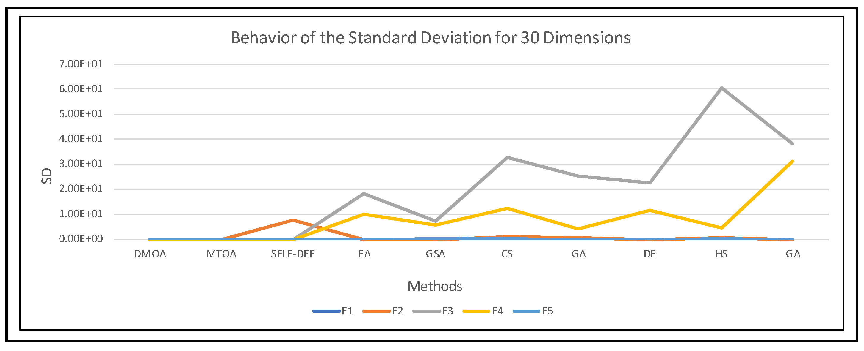
| 30 Dimensions | ||||||||||
|---|---|---|---|---|---|---|---|---|---|---|
| Method | DMOA | MTOA | SELF-DEFENSE | FA | GSA | |||||
| Func | Mean | SD | Mean | SD | Mean | SD | Mean | SD | Mean | SD |
| F1 | 2.79 × 10⁻⁷ | 2.36 × 10⁻⁷ | 4.72 × 10⁻⁸ | 1.98 × 10⁻⁸ | 1.53 × 10⁻⁸ | 6.42 × 10⁻⁸ | 1.99 × 10⁻³ | 5.13 × 10⁻⁴ | 9.45 × 10⁻¹⁷ | 3.81 × 10⁻¹⁷ |
| F2 | 6.51 × 10⁻⁸ | 3.74 × 10⁻⁸ | 1.67 × 10⁻⁸ | 1.06 × 10⁻⁸ | 4.98 × 100 | 7.54 × 100 | 1.06 × 10⁻² | 1.42 × 10⁻³ | 7.16 × 10⁻⁹ | 1.69 × 10⁻⁹ |
| F3 | 2.88 × 10⁻⁸ | 2.40 × 10⁻⁸ | 1.29 × 10⁻⁸ | 7.35 × 10⁻⁹ | 4.92 × 10⁻⁹ | 4.02 × 10⁻⁹ | 3.41 × 101 | 1.84 × 101 | 2.70 × 101 | 7.45 × 100 |
| F4 | 3.34 × 10⁻⁷ | 2.44 × 10⁻⁷ | 3.85 × 10⁻⁸ | 1.69 × 10⁻⁸ | 4.22 × 10⁻⁴ | 1.61 × 10⁻³ | 3.71 × 101 | 9.92 × 100 | 2.63 × 101 | 5.69 × 100 |
| F5 | 4.01 × 10⁻⁷ | 3.75 × 10⁻⁷ | 5.62 × 10⁻⁸ | 2.45 × 10⁻⁸ | 1.94 × 10⁻⁴ | 6.99 × 10⁻⁴ | 3.38 × 10⁻³ | 1.59 × 10⁻³ | 3.19 × 10⁻² | 3.06 × 10⁻² |
| Method | CS | GA | DE | HS | GA | |||||
| Func | Mean | SD | Mean | SD | Mean | SD | Mean | SD | Mean | SD |
| F1 | 2.13 × 10⁻⁴ | 2.18 × 10⁻⁴ | 4.20 × 10⁻³ | 3.88 × 10⁻³ | 1.59 × 10⁻³ | 4.28 × 10⁻⁴ | 3.66 × 10⁻² | 5.95 × 10⁻³ | 9.28 × 10⁻⁵ | 5.09 × 10⁻⁵ |
| F2 | 2.15 × 100 | 1.09 × 100 | 4.71 × 10⁻¹ | 5.22 × 10⁻¹ | 9.78 × 10⁻³ | 1.31 × 10⁻³ | 2.32 × 100 | 4.68 × 10⁻¹ | 2.62 × 10⁻³ | 5.91 × 10⁻⁴ |
| F3 | 2.88 × 101 | 3.29 × 101 | 1.59 × 101 | 2.54 × 101 | 3.38 × 101 | 2.25 × 101 | 1.02 × 10+2 | 6.06 × 101 | 5.06 × 101 | 3.83 × 101 |
| F4 | 5.34 × 101 | 1.22 × 101 | 1.31 × 101 | 4.13 × 100 | 3.72 × 101 | 1.17 × 101 | 2.89 × 101 | 4.68 × 100 | 8.76 × 101 | 3.13 × 101 |
| F5 | 2.72 × 10⁻² | 5.86 × 10⁻² | 4.43 × 10⁻⁴ | 5.20 × 10⁻⁴ | 3.18 × 10⁻³ | 1.57 × 10⁻³ | 2.71 × 10⁻² | 2.34 × 10⁻² | 1.93 × 10⁻³ | 3.33 × 10⁻³ |
| 50 Dimensions | ||||||||||
|---|---|---|---|---|---|---|---|---|---|---|
| Method | DMOA | MTOA | SELF-DEFENSE | FA | GSA | |||||
| Func | Mean | SD | Mean | SD | Mean | SD | Mean | SD | Mean | SD |
| F1 | 4.24 × 10⁻⁷ | 2.89 × 10⁻⁷ | 4.58 × 10⁻⁸ | 2.02 × 10⁻⁸ | 1.78 × 10⁻⁷ | 7.25 × 10⁻⁵ | 1.15 × 10⁻² | 3.20 × 10⁻³ | 4.54 × 10⁻¹⁶ | 2.19 × 10⁻¹⁶ |
| F2 | 5.64 × 10⁻⁸ | 4.83 × 10⁻⁸ | 1.72 × 10⁻⁸ | 1.18 × 10⁻⁸ | 3.77 × 10⁻⁸ | 8.79 × 100 | 2.49 × 10⁻² | 3.66 × 10⁻³ | 7.27 × 10⁻² | 2.73 × 10⁻¹ |
| F3 | 2.25 × 10⁻⁸ | 2.16 × 10⁻⁸ | 3.77 × 10⁻⁹ | 3.30 × 10⁻⁹ | 2.27 × 10⁻⁸ | 5.90 × 10⁻⁵ | 5.85 × 101 | 3.18 × 101 | 7.62 × 101 | 3.50 × 101 |
| F4 | 3.49 × 10⁻⁷ | 3.02 × 10⁻⁷ | 3.71 × 10⁻⁸ | 1.89 × 10⁻⁸ | 1.81 × 10⁻⁷ | 9.60 × 10⁻³ | 7.45 × 101 | 2.47 × 101 | 5.07 × 101 | 1.26 × 101 |
| F5 | 3.15 × 10⁻⁷ | 3.36 × 10⁻⁷ | 5.67 × 10⁻⁸ | 2.47 × 10⁻⁸ | 3.22 × 10⁻⁷ | 5.97 × 10⁻² | 7.01 × 10⁻³ | 2.04 × 10⁻³ | 1.24 × 100 | 2.44 × 10⁻¹ |
| Method | CS | GA | DE | HS | GA | |||||
| Func | Mean | SD | Mean | SD | Mean | SD | Mean | SD | Mean | SD |
| F1 | 9.90 × 10⁻¹ | 7.89 × 10⁻¹ | 1.77 × 100 | 6.66 × 10⁻¹ | 7.19 × 10⁻³ | 1.79 × 10⁻³ | 3.54 × 10⁻¹ | 7.94 × 10⁻² | 1.77 × 100 | 6.66 × 10⁻¹ |
| F2 | 4.84 × 100 | 1.32 × 100 | 1.73 × 100 | 3.15 × 10⁻¹ | 1.86 × 10⁻² | 2.05 × 10⁻³ | 3.12 × 100 | 3.14 × 10⁻¹ | 1.73 × 100 | 3.15 × 10⁻¹ |
| F3 | 2.28 × 10+2 | 1.27 × 10+2 | 2.96 × 101 | 5.07 × 101 | 4.80 × 101 | 7.41 × 10⁻¹ | 2.04 × 10+2 | 7.36 × 101 | 2.96 × 101 | 5.07 × 101 |
| F4 | 1.15 × 10+2 | 2.07 × 101 | 3.70 × 101 | 7.63 × 100 | 7.81 × 101 | 2.27 × 101 | 8.26 × 101 | 8.04 × 100 | 3.70 × 101 | 7.63 × 100 |
| F5 | 6.21 × 10⁻¹ | 2.13 × 10⁻¹ | 5.05 × 10⁻² | 1.61 × 10⁻² | 5.91 × 10⁻³ | 1.09 × 10⁻³ | 1.22 × 100 | 7.73 × 10⁻² | 5.05 × 10⁻² | 1.61 × 10⁻² |
Publisher’s Note: MDPI stays neutral with regard to jurisdictional claims in published maps and institutional affiliations. |
© 2022 by the authors. Licensee MDPI, Basel, Switzerland. This article is an open access article distributed under the terms and conditions of the Creative Commons Attribution (CC BY) license (https://creativecommons.org/licenses/by/4.0/).
Share and Cite
Carreon-Ortiz, H.; Valdez, F.; Castillo, O. A New Discrete Mycorrhiza Optimization Nature-Inspired Algorithm. Axioms 2022, 11, 391. https://doi.org/10.3390/axioms11080391
Carreon-Ortiz H, Valdez F, Castillo O. A New Discrete Mycorrhiza Optimization Nature-Inspired Algorithm. Axioms. 2022; 11(8):391. https://doi.org/10.3390/axioms11080391
Chicago/Turabian StyleCarreon-Ortiz, Hector, Fevrier Valdez, and Oscar Castillo. 2022. "A New Discrete Mycorrhiza Optimization Nature-Inspired Algorithm" Axioms 11, no. 8: 391. https://doi.org/10.3390/axioms11080391