1. Introduction
Distribution theory provides useful tools in describing and identifying the model of occurred events and predicting next events. Recently, several generators of probability distributions have been introduced by many researchers in the statistical literature. Some well-known generators are the Marshall–Olkin generated (MO-G) by [
1], beta-G by [
2], Kumaraswamy-G (Kw-G) by [
3], Weibull-G by [
4], exponentiated half-logistic-G by [
5], Lomax-G by [
6], and polar-generalized normal distribution by [
7], among others.
A favorite technique in expanding statistical distributions is the method introduced by [
8], who have introduced the generalized log-logistic (GLL-G) class of distributions. The cumulative distribution (cdf) function of this class based on underline cdf
G, is given by
where
and
denote the survival function. This class has named by Odd log-logistc (OLL-G) and several extensions of this class were introduced. Kumaraswamy Odd log-logistic due to [
9], beta odd log-logistic due to [
10], odd burr generalized class due to [
11], Topp–Leone odd log-logistic due to [
12], generalized odd log-logistic due to [
13], new odd log-logistic due to [
14] and odd log-logistic logarithmic by [
15].
The purposes of this work are two fold. We first introduce a general and versatile class of distributions in terms of compounding the arctan function and cdf defined in (
1). This model is referred to as the arctan odd log-logistic-G (ATOLL-G) distribution. The second purpose of this work lies in the study of two sub-models of the general ATOLL-G model via classical and Bayesian approaches. Further, we study the corresponding regression model derived from sub-model which is defined based on the Weibull distribution. First, certain statistical and reliability properties of the ATOLL-G distribution are derived in a general setting. Then, we establish two special cases of ATOLL-G by using the Weibull and normal distributions instead of the parent distribution
G. These models are called ATOLL-W and ATOLL-N distribution, respectively. We also provide a discussion for the ATOLL-W regression model via log-transformation of ATOLL-W (LATOLL-W) distribution. Furthermore, we obtain Bayesian and maximum likelihood estimates of the parameters of proposed models via real examples.
For Bayesian inference, we consider several asymmetric and symmetric loss functions such as squared error loss, modified squared error, precautionary, weighted squared error, linear exponential, general entropy, and
K-loss functions to estimate the parameters of the LATOLL-W regression model. Further, making use of the independent prior distributions, Bayesian
credible and highest posterior density (HPD) intervals (see [
16]) are provided for each parameter of the proposed model. In addition, a simulation study is performed to investigate Maximum Likelihood Estimators (MLEs) of consistency.
The rest of the manuscript is organized as follows. In
Section 2, we introduce a new class of distributions called arctan odd log-logistic-G (ATOLL-G) distribution. Some structural properties of the ATOLL-G distribution such as the hazard function, quantiles, asymptotics and some useful expansions of the proposed model are given in a general setting in
Section 3. In
Section 4, two special cases of this class is considered by employing Weibull and normal distributions as the parent distribution. The ATOLLW regression model and its Bayesian inference are presented by considering seven well-known loss functions in
Section 5. In
Section 6, we study the performance of the maximum likelihood estimates of the parameters of ATOLLW distribution via Monte Carlo simulation to investigate the mean square error and bias of the maximum likelihood estimators. In
Section 7, the supremacy of the ATOLLN and ATOLLW models to some challenger models is exhibited via several selection model criteria by analyzing Data 1 and Data 2 real examples, respectively. Further, we fit the LATOLLW regression model to heart transparent dataset and compare its efficiency with some competitor models. We also provide the numerical results of Bayesian inference and related plots to posterior samples for heart transplant data in this Section. Finally, the paper is concluded in
Section 8.
5. The ATOLLW Regression Model
The survival regression model is one of well-known models in survival analysis. Sometimes for analyzing a lifetime variable, there are auxiliary information (as independent variables) that help us to explore the lifetime variable more precisely. More recently, by considering the class of location statistical distributions, different regression models have been introduced in the applied statistical literature (for example see [
13,
21]). The log-odd log-logistic Weibull regression model for censored data was introduced by [
22] in terms of odd log-logistic Weibull distribution. Further, Cordeiro et al. [
23] introduced a general regression model based on the Burr XII system of densities and also the log-odd power Cauchy–Weibull regression proposed by [
24].
Let
X be a variable with pdf ATOLL-W defined in (
12). Making use of the log transformation
, the pdf of transformed variable
Y is given by:
where
is a scale,
is a shape and
is a location parameter. The model in (
16) is referred to as log-ATOLL-W (LATOLL-W) distribution, and it is briefly shown by
. The survival function of
Y is:
Let
be the standardized random variable having pdf,
The ATOLL-W regression is defined by:
where
is parameter vector of regression model,
is covariate variable vector and
is an error of regression model with density
. Further, under assumptions
, where
denotes log-censoring and
follows (
16), and represent the log-lifetime. Let
r is the number of uncensored observations, then the log-likelihood function for
in terms of sets
F (set of individuals with log-lifetime) and
C (set of individuals with log-censoring) is given by:
where
,
. For example, we can use the optim function of R software to obtain the MLE of
by maximizing (
19).
5.1. Residual
The martingale and modified deviance residuals (mdr) for the LATOLL-W regression are given respectively by:
where
, and
When the regression model is well-fitted to a given data, the mdr are normally distributed with zero men and unit variance.
5.2. Bayesian Inference of Regression Model
In this section, we consider the Bayesian inference of the parameters for the survival regression model, which is discussed in
Section 5. Let the parameters
,
and
of the LATOLLW distribution have independent prior distributions as:
where
a,
b,
c,
d,
e and
f are positive and
,
. Under these assumptions, the joint prior density function is formulated as follows:
where
.
Here, we consider several asymmetric and symmetric loss functions including: squared error loss function (SELF), modified squared error loss function (MSELF), weighted squared error loss function (WSELF),
K-loss function (KLF), linear exponential loss function (LINEXLF), precautionary loss function (PLF) and general entropy loss function (GELF). For more details, see [
25] and the references therein. In
Table 1, we provide a summary of these loss functions and associated Bayesian estimators and posterior risks.
For more details see [
26]. Let
be a function defined as:
Since the joint posterior distribution
is formulated as:
Therefore, the joint posterior density is given by:
where
is a known matrix that contains the auxiliary variables,
and
K is given as:
where the outer integration stands for parameter vector
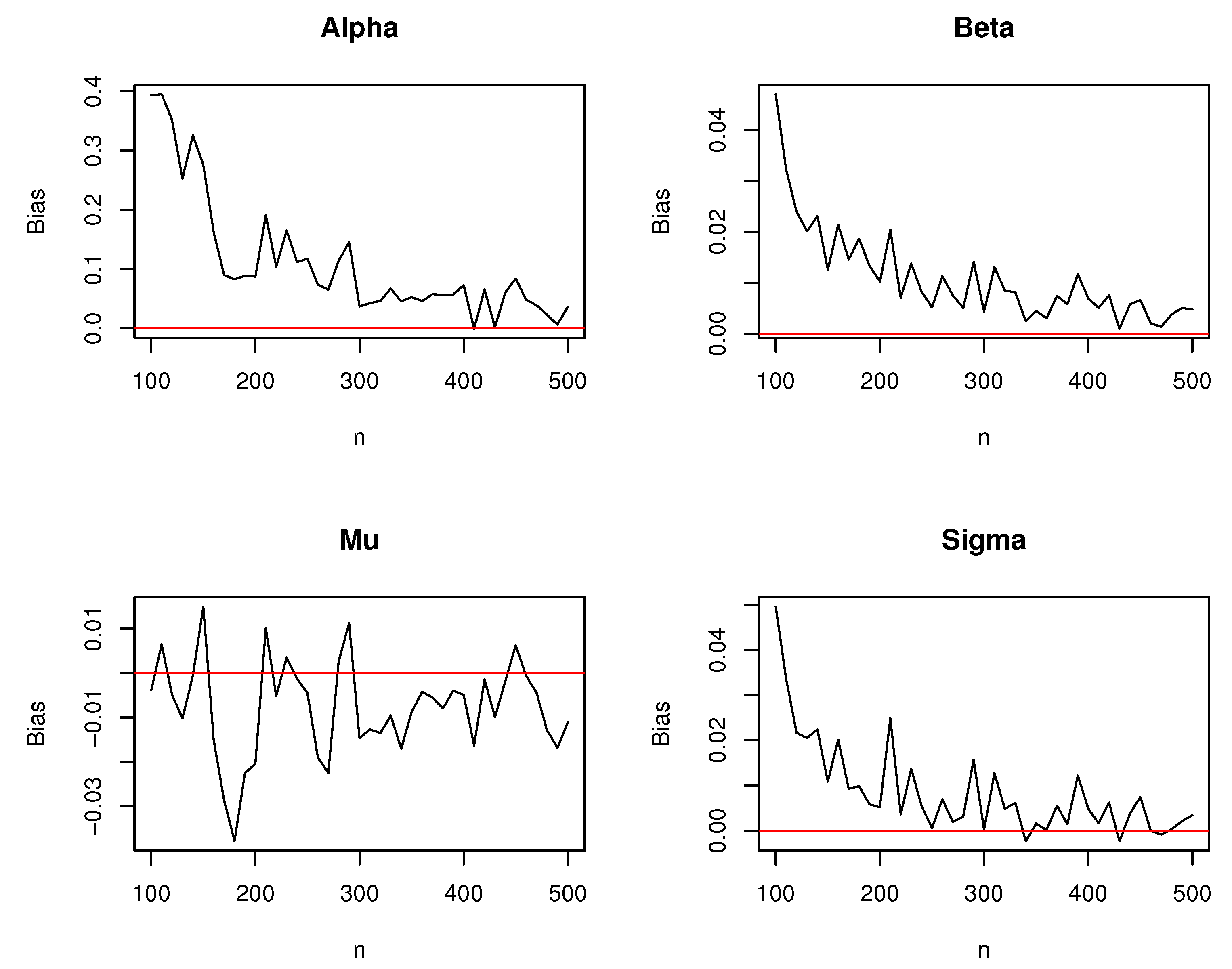
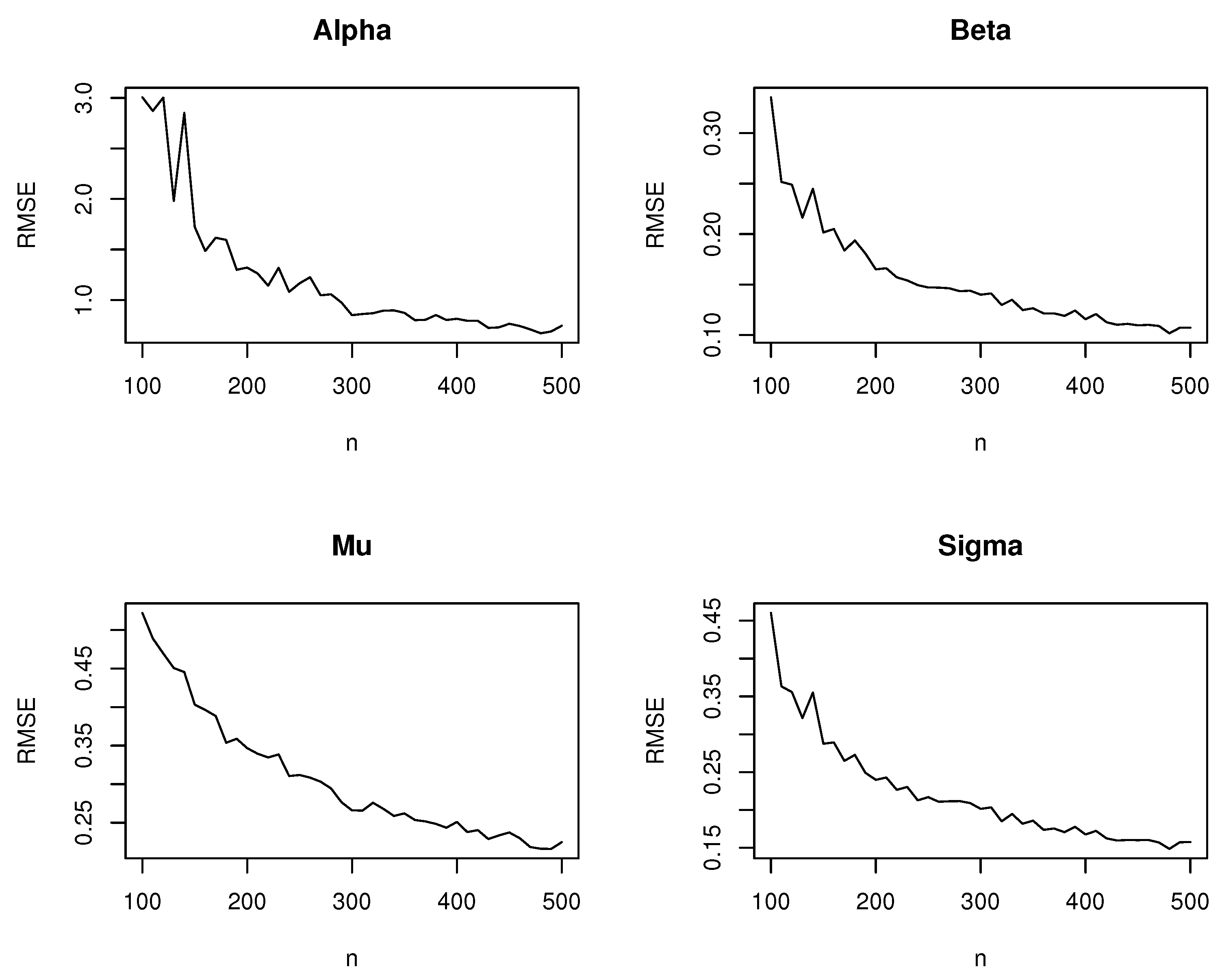
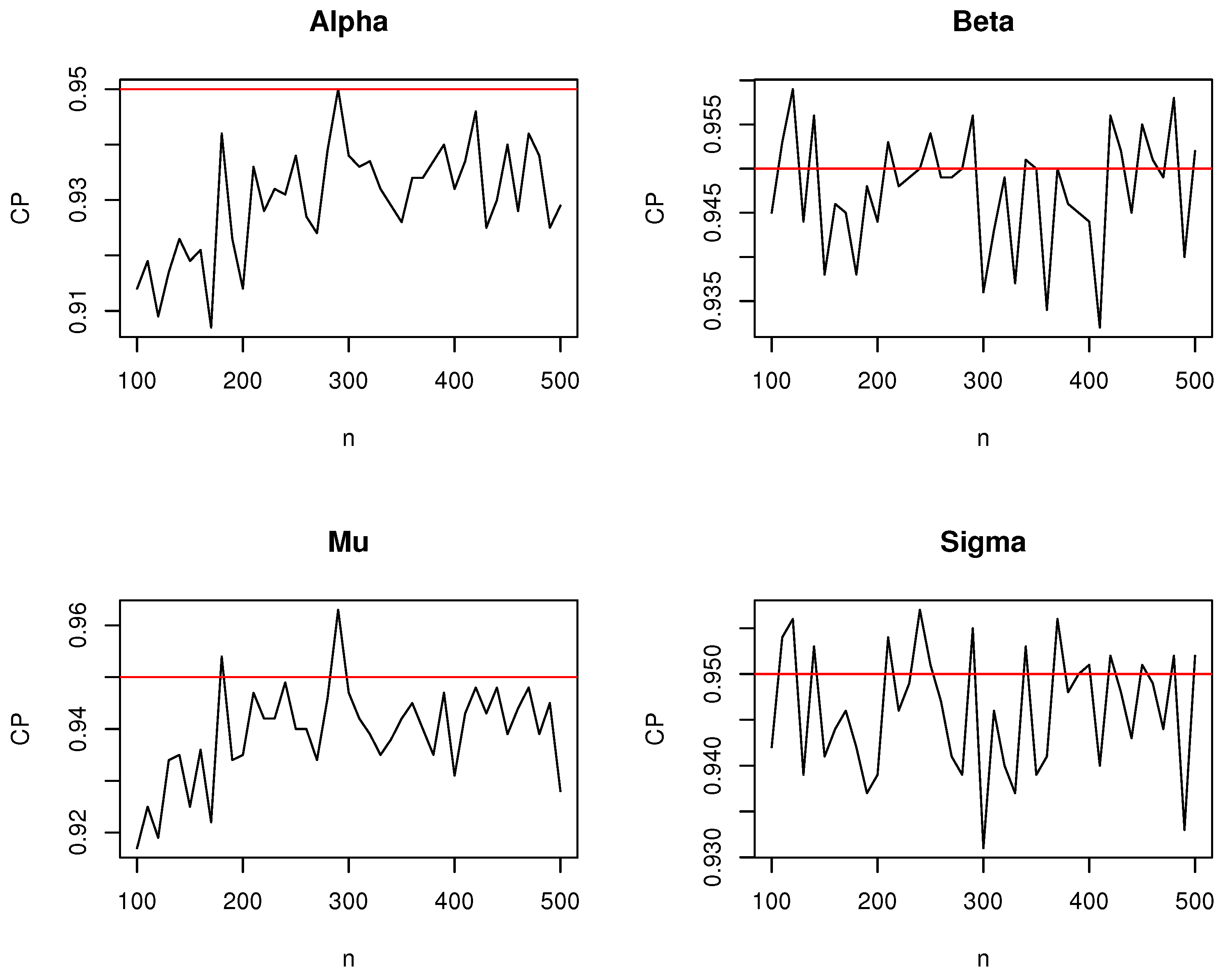
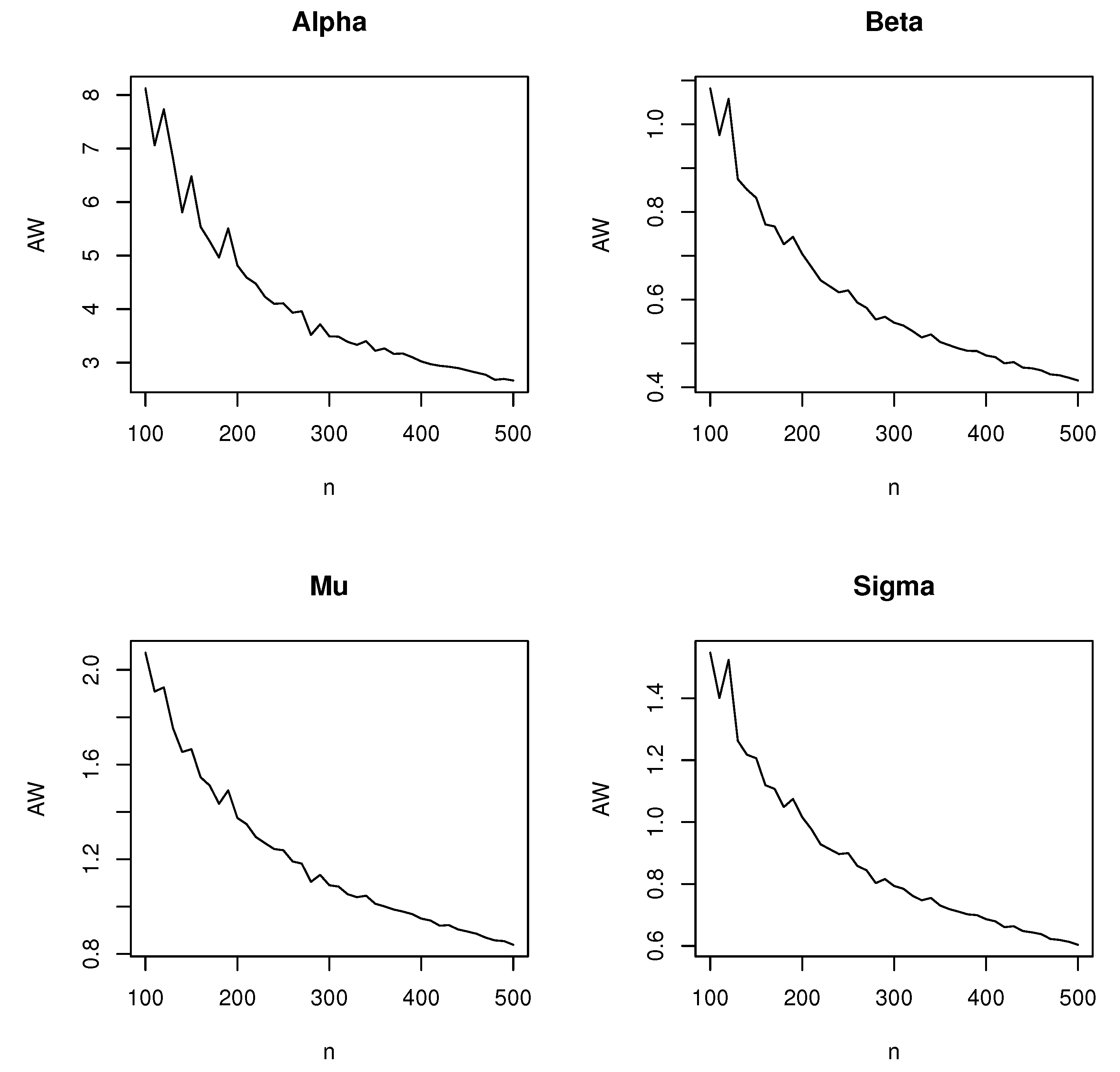
6. Simulation
Here, we examine the performance of the maximum likelihood estimates associated to the ATOLLN
distribution in (
14) with respect to sample size
n. The simulation study is performed via the Monte Carlo procedure as follows:
Generate 5000 samples of size
n for the ATOLLN
distribution by using the relation (
8);
Compute the maximum likelihood estimates of parameter vector for the one thousand samples, say , for ; ;
Compute diagonal elements of inverse Fisher information matrix , ; , where j stands for -th elements of parameter vector ;
Compute the average biases (AB), mean squared errors (MSR), coverage probabilities (CP) and average lengths (AW) given by:
and
where
is the standardized normal quantile at
confidence level and
denotes the indicator function.
We repeated these steps based on the sample sizes
for the one set of selected values of parameter vector as
.
Figure 4,
Figure 5,
Figure 6 and
Figure 7 show how the AB, MSR, CP and the AW vary with respect to
n. These results show that the average biases, mean-squared errors and average lengths for each parameter decrease to zero as
Additionally, the CP vary with respect to
n. The associated results of CP corresponds to the nominal coverage probability of
for two parameters
and
. The level of CP for the two parameters
and
are increasing when
n is increased to the level of
.
7. Applications
In this part, we present three applications to investigate the efficiency and flexibility of two sub-classes distributions which formerly defined in
Section 4 and
Section 5. In the first two applications, we present some numerical and graphical results for fitting the special sub-models defined in
Section 4. The third application is associated with a survival regression analysis of the ATOLL-W regression model presented in
Section 5.
For the first two applications, the goodness-of-fit statistics including the Cramér–von Mises (
) and Anderson–Darling (
) test statistics are adopted to compare the fitted models (see [
27,
28,
29] for more details). The smaller values of
and
present the better fit to the data. For the sake of comparison, we also consider the Kolmogorov–Smirnov (K-S) statistic and its corresponding
p-value and the minus log-likelihood function (
) for the sake of comparison [
28,
29]. For the third application (covariate censored data), we adopt the AIC and BIC statistics to compare the fitted models since the
and
statistics are not suitable for censored data.
For the first application, we take the ATOLLN distribution and, for comparison purposes, we fitted the following models to the above datasets:
where , , , and .
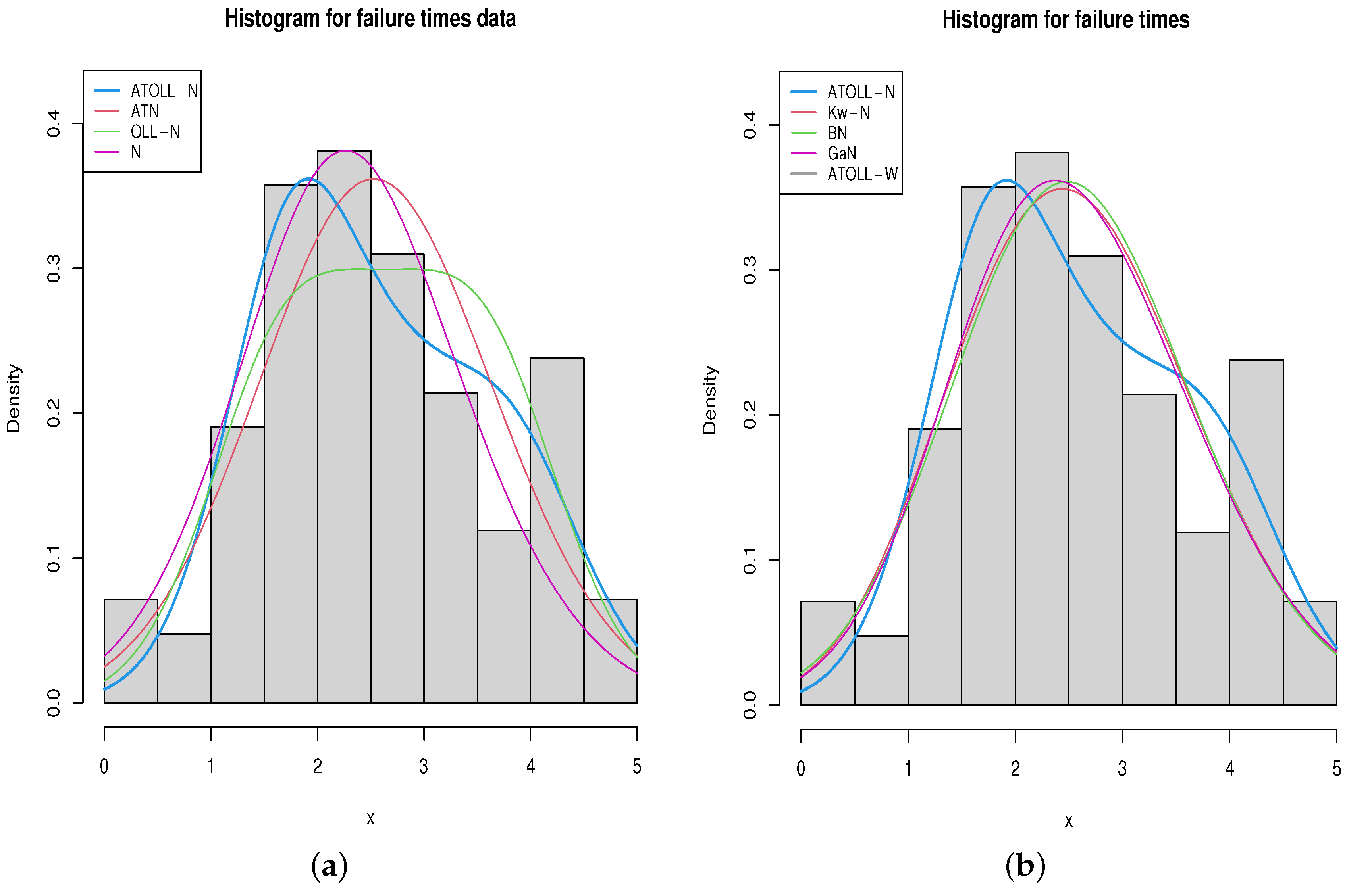
7.1. Failure Times Data
Data 1: First, we analyze the 84 failure times of a particular windshield device. These data were also studied by [
32,
33].
The MLEs of the parameters, standard errors (SE) (in parentheses) and the goodness-of-fit statistics for failure times data are reported in
Table 2. One can see that the ATOLLLN model outperforms all the fitted competitive models under these statistics.
The fitted densities and histogram of the data are displayed in
Figure 8. For failure times, we note that the fitted ATOLLN distribution best captures the empirical histogram.
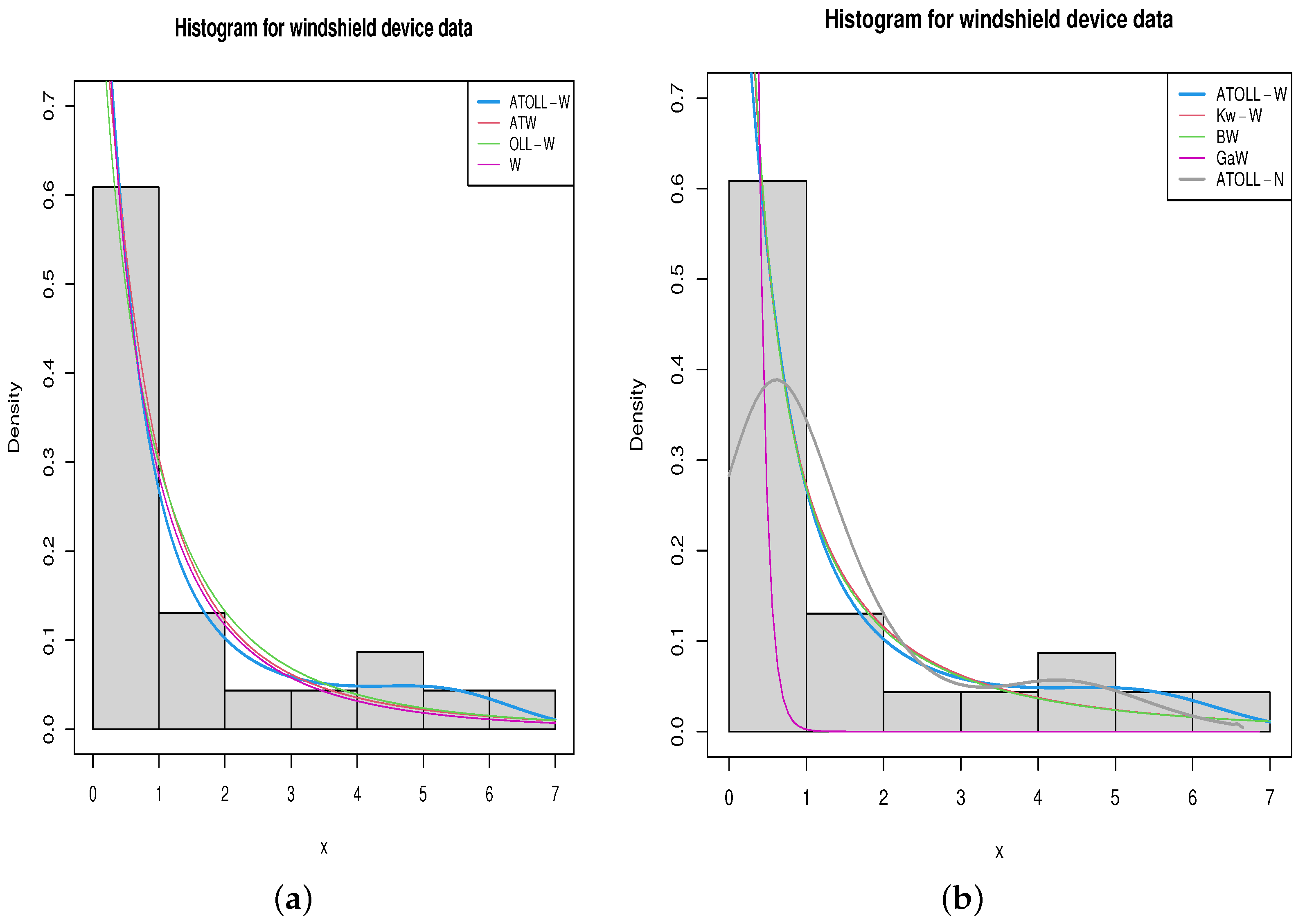
7.2. Windshield Device Data
Data 2: Second, we examine 23 failure times of a particular windshield device. These data were also studied by [
32,
33]. The data, referred as windshield device, are: 2.160, 0.746, 0.402, 0.954, 0.491, 6.560, 4.992, 0.347, 0.150, 0.358, 0.101, 1.359, 3.465, 1.060, 0.614, 1.921 4.082, 0.199, 0.605 0.273 0.070 0.062 5.320.
Here, we fit the ATOLLW distribution and some of its sub-models, odd log-logistic Weibull (OLL-W), beta Weibull (BW), Kumaraswamy–Weibull (kwW), gamma Weibull (GaW) and exponentiated Weibull (EW) distributions to the windshield device data. Similar numerical results are provided in
Table 3 for windshield device data as well as data failure times data. It is immediately seen that the ATOLLW model outperforms all the fitted competitive models under the model selection criteria presented for the first data application.
The fitted densities and histogram of the windshield device data are displayed in
Figure 9. This figure shows that the fitted ATOLLW distribution best captures the empirical histogram among the considered competitor models.
We note that the ATOLLN and ATOLLW models outperform all the fitted competitive models under the selected criterion for the datasets’ failure times and windshield device, respectively.
7.3. Third Application: Regression Analysis
Survival regression analysis has been developed in several forms. One of them is the non-parameteric, where Kaplan–Meier estimation [
34] is highlighted. The Kaplan–Meier estimate is a common way of obtaining the survival curve using probabilities of an event’s occurrence at a time. In this section, we provided a parametric approach as a counterpart, where we fit the LATOLLW regression to the heart transplant data. The current data are available in a survival package of R software. The considered survival regression model based on response variable
and covariate variables (
) is formulated as:
where
is distributed as the LATOLLW distribution and the covariate random variables are described as:
7.3.1. Parameter Estimation
A summary of model fitting based on MLE discussion for the heart transplant data is provided in
Table 4. We fit the LATOLLW regression model to this dataset and compare the results with LBXII-W, LOLLW and log-Weibull distributions. For more details about these competitor models, see [
23]. We also consider another alternative models such as a log-log mean Weibull (LLMW) regression proposed by [
35] and log exponential-Pareto (LEP) regression model proposed by [
36]. The estimated parameters, standard errors (given in parentheses) and AIC and BIC measures as well as corresponding p-values in
are reported in
Table 4. We conclude that the estimated regression parameters are statistically significant at the
level.
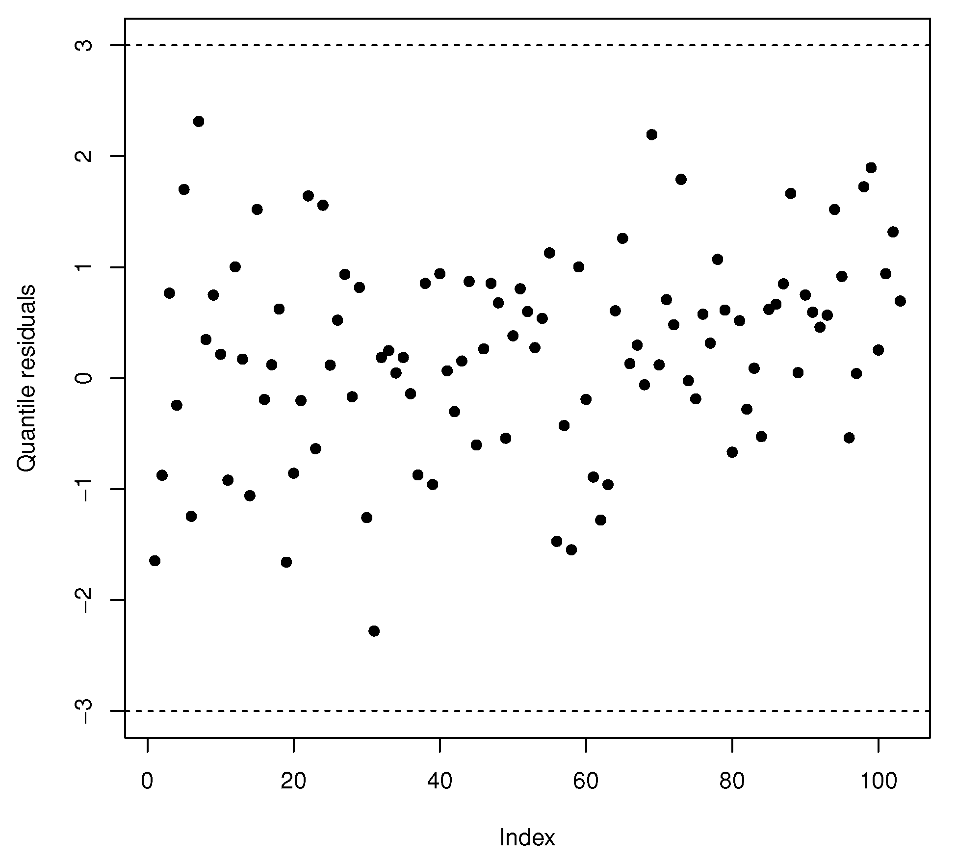
7.3.2. Results of Residual Analysis
The suitability of the fitted LATOLLW regression model is evaluated by residual analysis. The plot of the modified deviance residuals is displayed in
Figure 10, which reveals that the fitted LATOLLW regression provides a good fit to the current data.
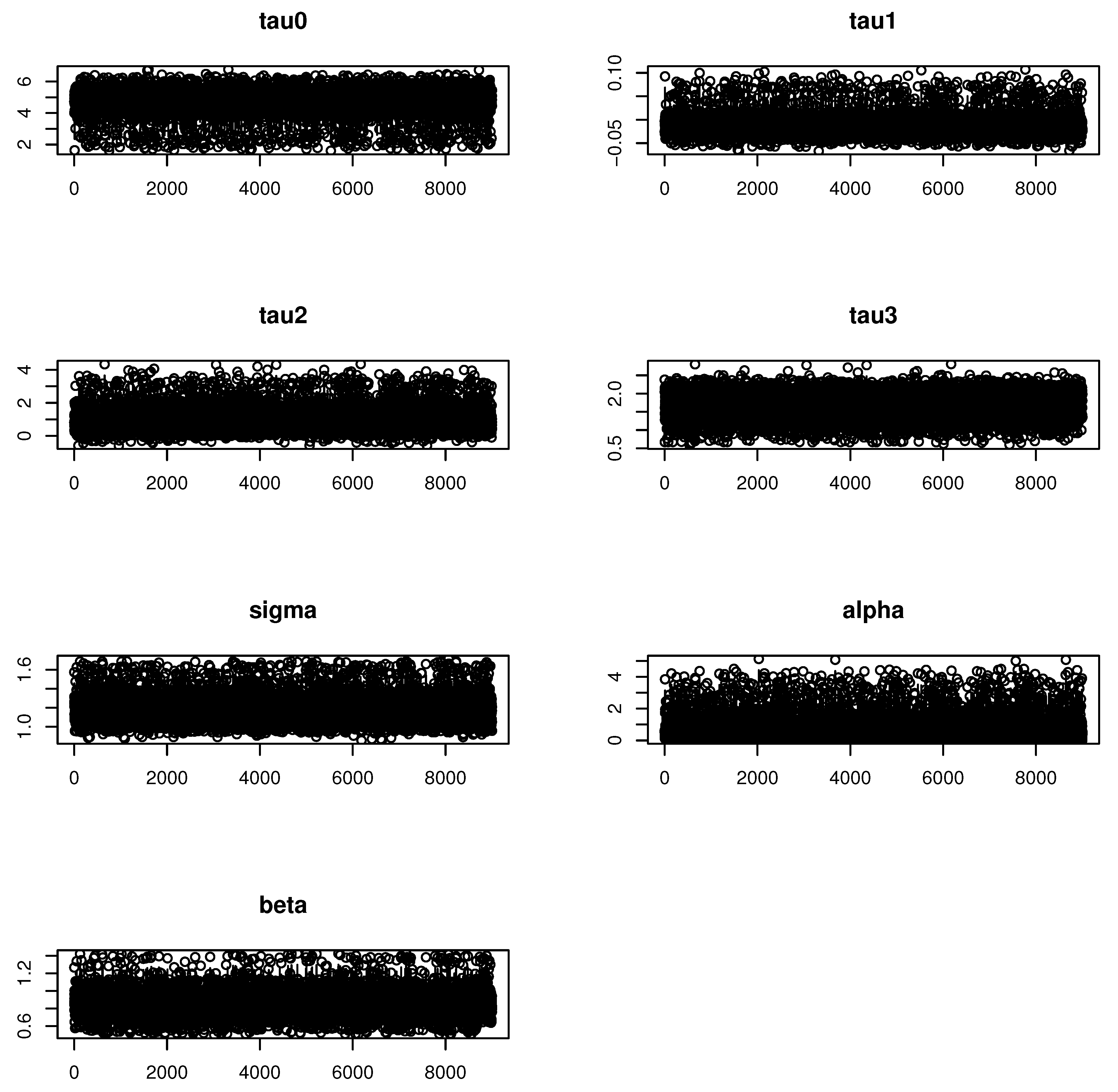
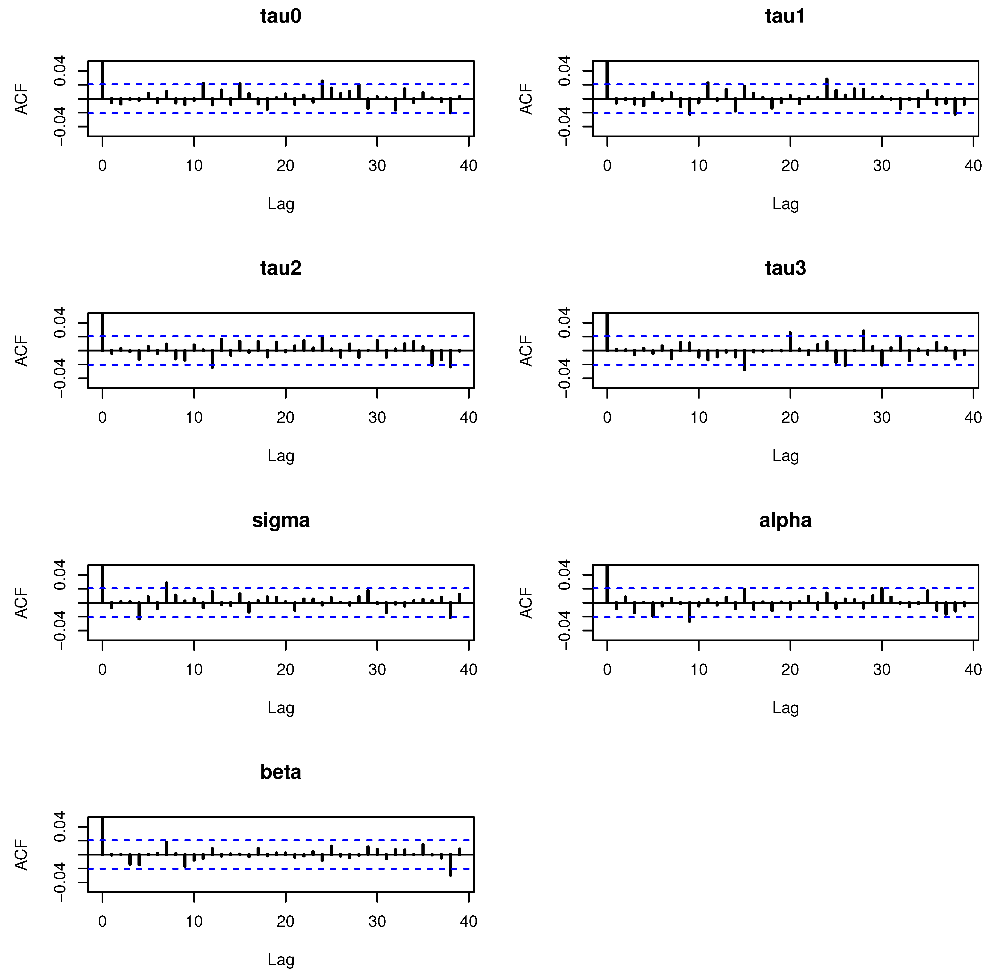
7.4. Bayesian Regression Analysis: Heart Transplant Data
From (
24), we can see that there is no explicit form for the Bayesian estimators under the loss functions considered in
Table 1, so we use Gibbs sampling technique and MCMC procedure based on 10,000 replicates to obtain Bayesian estimators for the heart transplant data. A summary of Bayesian analyses (point and interval estimations with related posterior risk) are reported in
Table 5 and
Table 6.
Table 6 provides
credible and HPD intervals for each parameter of the LATOLLW distribution. Moreover, we provide the posterior summary plots in
Figure 11,
Figure 12 and
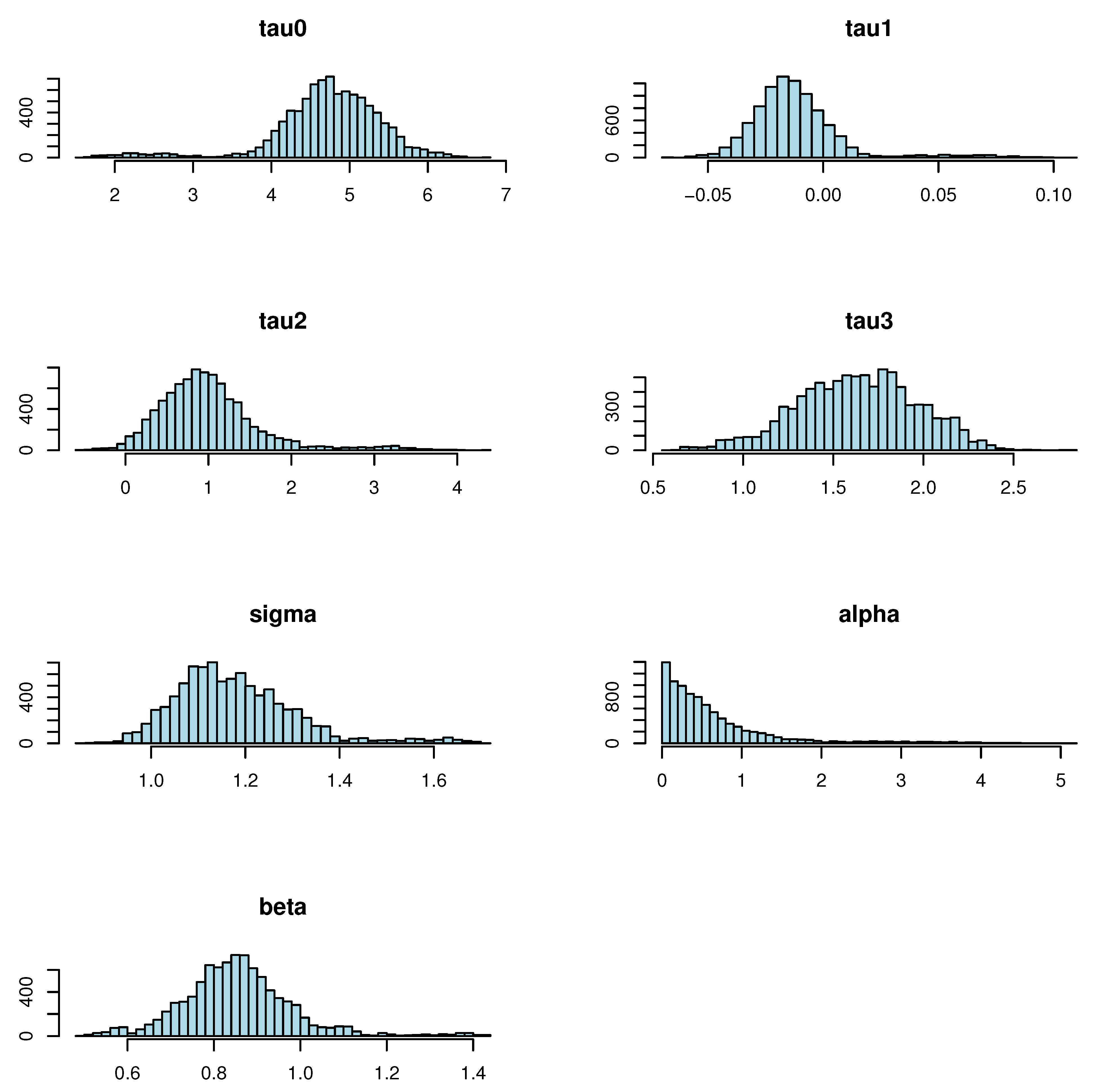
Figure 13. These plots confirm that the convergence of sampling process occurred.


