Article

Some Generalized Results on Grey Number Operations Based on Liu-Lin Axioms of Greyness Degree and Information Content

1
Department of International Trade and Business, İstanbul Topkapı University, İstanbul 34020, Turkey
2
Department of Management Information Systems, İstanbul Topkapı University, İstanbul 34020, Turkey
*
Author to whom correspondence should be addressed.
Axioms 2022, 11(9), 424; https://doi.org/10.3390/axioms11090424
Submission received: 11 July 2022 / Revised: 17 August 2022 / Accepted: 19 August 2022 / Published: 24 August 2022

Abstract

:
In this manuscript, with grounding in Liu–Lin axioms of greyness degree and information content, we provide new results that relate to these concepts in consideration of a number of mathematical operations over a sequence of grey numbers. In particular, we derive greyness degree results of summation, conic combination, and convex combination of a sequence, as well as inverse of a number and normalization of a number over a sequence. Then, we turn our attention to prove information content results for the union and intersection of a sequence. We illustrate our results by using a simple Monte Carlo simulation in the multi-attribute decision-making context, and by using an interesting dice-rolling experiment. Through our analysis, we also provide some new definitions, such as for conic combination, convex combination, normalization, and union and intersection operations. The novelty of the derived results in this study is that they can help researchers and practitioners of grey systems in tracking probable intensifications and reductions in the greyness degree in successive application steps of their working methods. Moreover, researchers are provided with two results to calculate information content for the union and intersection of grey numbers in an uncomplicated manner.

1. Introduction

Through introducing a primary paper, Deng [1] initiated the paradigm of grey systems, which stand for a class of complex systems under partially known and imprecise system parameters. In a series of following accounts [2,3,4,5], he promoted an alternate system of thinking and its basic principles for uncertainty modelling under this paradigm. Today, we recognize that the theoretical basis of grey systems and their engineering and socio-technical inferences carry forward well in a variety of applicable models. The grey system continues growing as an independent theory encompassing several domains, such as grey prediction, grey decision making, grey control, grey relational and generating spaces, and grey input-output analysis. Our current manuscript is not meant to be an exhaustive analysis of inquiries into theory and applications of the grey system in the first place; hence, we summarized a selection of studies in this body of work in Table 1 for interested readers. In this table, we reserved three columns after the source information: the features column lists which attribute or trait the paper brings to the interest of the readers; the methods and theories column records which celebrated method, applicable concept, or theory is utilized in the analysis; and the cases and illustrations column is reserved to specify the outline chosen to verify study findings. For notable assessments on the current state of developments and future prognoses on grey systems research, one may also refer to in-depth reviews [6,7,8,9].
The essential element of a grey system is the grey number. It stands for a number whose cardinality is not explicitly known, yet its span is known as a closed interval. As such, the conventional representation of a grey number is carried out by determining two values, referred to as the left and right projections, delimiting this range. There exist some other representations; for example, there are discrete [13] and kernel representations [17,28,64] of grey numbers. Nevertheless, in this paper, we will limit our attention to the conventional representation of grey numbers, i.e., representation as closed intervals.
When used to typify quantitative phenomena, any grey number has an intrinsic character attached to it, namely, its greyness degree, or simply the greyness. Greyness degree revolves around what we can not know about a parameter of concern when represented by a particular grey number, i.e., it is a measure of the representation ability of a grey number. Let z denote a grey number, and suppose we have an estimate of the temperature on a given day represented by z 1 = 17 , 24 on a Celsius scale. It is apparent that we do not have a good estimate. All we know is that the weather will either be chilly or mild, or of some warmth that is in between these two conditions, giving no practical information for our everyday purposes, for example, in deciding whether to go for a picnic or not. In this case, a considerable greyness degree is attached to this information, that is, to the grey number z 1 . Suppose now we have an estimate z 2 = 37 , 44 about the temperature on a different day. Obviously, this estimate is much more valuable than z 1 , as it provides a useful body of information to us. We definitely know that the weather will be very hot for any practical purpose. Thus, the greyness degree attached to z 2 should be smaller than that attached to z 1 in this case. Observe from this example that, although the spans of these numbers over the Celsius scale are of the same length, their ability to convey information is different.
On the other hand, there exists yet another essential attribute associated with grey numbers, namely, the information content. Information content held within a grey number is an extent which shows awareness of the researcher about a particular grey system under study. Liu and Lin [65] argue that this measure can not be irrelevant to the background where the grey number of concern is initially introduced. Had this been the case, it would be impossible to assess the scope of information that is conveyed by the grey number. In order to see this, suppose we introduce the grey number z 3 = 5 , 12 with no background evidence attached. We do not know whether the information carried by z 3 is useful or not. Now, let us introduce a background which communicates that the grey number is an estimate of percentage GDP growth of a particular country. Instantly, we retain a fair amount of information in attaining the grey number z 3 .
These two examples really show the existence of a collection of unique principles that make up the concepts of greyness degree and information content. One may trace these roots by surveying the axiomatic background of greyness degree and information content established by Liu [12], and later by Liu and Lin [65].
Research on greyness degree and information content is in its infancy. In particular, studies on greyness degree and information content results that consider basic mathematical operations of grey numbers are very limited. These preliminary results are merely constrained to the papers of Liu [12] and Liu and Lin [65] under the interval representation of grey numbers; Yang’s [13] treatment of discrete grey numbers; and a subsequent stream of research by Yang and Liu [17,28], and by Liu et al. [64] under the kernel representation of grey numbers. In these accounts, mathematical operations are analyzed by considering two grey numbers at a time.
What remains necessary to develop is a collection of greyness degree results that will work when a group or sequence of grey numbers is considered. This is because researchers should be able to track the amplifications and reductions in greyness degree in successive application steps of the working method through their analyses. In the current paper, we aim to generalize the above results in this manner, under the interval representation of grey numbers with some new additions that consider distinct operations such as the summation of a sequence of grey numbers, their conic combination, their convex combination, the inverse of a grey number, and the normalization over a sequence of grey numbers. Although these operations are very common in many grey systems, for example in grey prediction systems, and as will be clear later in this paper, grey decision-making systems, currently we do not know the effect of application steps on greyness degree as one continues with these necessary operations while analyzing such systems. Similarly, in considering the information content, we bring in two general results that relate to the union and intersection of a sequence of grey numbers.
With these aspirations in mind, this manuscript is organized in the following manner. In Section 2 and Section 3, we first provide a brief overview of Liu–Lin axioms on the greyness degree of grey numbers, and then we develop our operation results through a number of theorems, respectively. Section 4 and Section 5 are organized in a similar manner, where we first provide a brief overview of Liu–Lin axioms on the information content of grey numbers, and then we develop our operation results through a number of theorems, respectively. Section 6 is reserved for illustrating our arguments that are related to greyness degree. In this line, we initially introduce a multiple-attribute decision-making case which will be useful for illustration purposes; subsequently, we demonstrate greyness degree results with the aid of a simple Monte Carlo simulation over this setting. Then, to illustrate our line of reasoning on the information content, we design a dice-rolling experiment in Section 7. Finally, we come to an end with our conclusions in Section 8.

2. Liu–Lin Axioms on Greyness Degree

In this section, we briefly overview the axiomatic background of the greyness degree concept.
Definition 1.
(Left and right projection; information field)
Let a 0 and b > a be two values delimiting the span of a grey number z = a , b . Then, a and b are called the left and right projections, respectively; and the closed interval a , b is called the information field of the grey number z .
Definition 2.
(Length of the information field [12])
Under the above notation, l z = b a is called the length of the information field of grey number z .
We also introduce the notation g z to denote the greyness degree of this number. We will maintain this convention throughout this paper unless otherwise stated. In two successive studies [12,65], Liu and Lin established five essential axioms regarding greyness degree.
Axiom 1.
g z 0 .
Their first axiom states that each grey number has an intrinsic greyness degree associated with it.
Axiom 2.
If l z = 0 , then g z = 0 .
The above axiom establishes that when the left and right projections of a grey number are equal, the number degenerates into a singleton whose greyness degree is zero. Then, the number is called a white number, i.e., its cardinality is known precisely.
Axiom 3.
If  a   or b , then g z .
This axiom indicates that when (left) right projection of a grey number is translated to (minus) infinity, the number degenerates into a black number whose greyness degree is illimitable.
Axiom 4.
g s · z = g z where s is a scalar.
Their fourth axiom specifies that multiplying a grey number with a scalar will not alter its greyness degree.
In grey systems theory, the function prescribing degrees of affinity for a grey number to assume particular values from its information field is called a weight function. In order to understand the fifth axiom of greyness degree, the following suggestion [65] is useful. When the weight function of a grey number is not known, the mean value whitenization is determined as follows:
z ^ = 1 2 · a + b
and can be substituted for the expected value of the grey number.
Axiom 5.
g z l z and g z 1 / z ^ where z ^ is the mean value whitenization of the grey number z .
This last axiom establishes the definition of greyness degree. The axiom literally states that the greyness degree of a grey number is directly proportional to the length of its information field, whereas it is inversely proportional to its associated expected value. Hence, based on this last axiom, the following definition of the greyness degree is recognized:
Definition 3.
(Greyness degree of a grey number [12,65])
g z = l z z ^ = 2 b a b + a .
Example 1.
We now revisit the temperature estimates instance under this definition. Greyness degrees for the aforementioned two temperature estimates z 1 and z 2 can be calculated as follows:
g z 1 = 2 24 17 24 + 17 = 0.341 ;       g z 2 = 2 44 37 44 + 37 = 0.172 .
This result shows that the greyness degree associated with grey number z 2 is considerably smaller than that attached to z 1 , as we have anticipated.

3. Greyness Degree Results of Mathematical Operations

In this section, we organize greyness degree results that relate to mathematical operations on a sequence of grey numbers. These include the following: summation, conic combination, convex combination, and normalization. The only exception is the inverse operation that is associated with a single grey number.
Theorem 1.
(Greyness degree of summation)
For a sequence of n grey numbers z i = a i , b i with a i 0 and b i > a i for i = 1 , , n :
g z 1 + + z n g z 1 + + g z n .
Proof of Theorem 1.
In generalizing the analysis for two grey numbers ([65], p. 35), for the L.H.S. of the inequality we have the following:
g z 1 + + z n = 2 b 1 + + b n a 1 + + a n b 1 + + b n + a 1 + + a n = 2 b 1 a 1 + + b n a n b 1 + + b n + a 1 + + a n = 2 b 1 a 1 b 1 + + b n + a 1 + + a n + + 2 b n a n b 1 + + b n + a 1 + + a n .
For the R.H.S. we have the following:
g z 1 + + g z n = 2 b 1 a 1 b 1 + a 1 + + 2 b n a n b n + a n .
A member-to-member comparison of (4) and (5) gives the following:
2 b i a i b 1 + + b n + a 1 + + a n 2 b i a i b i + a i ;   i = 1 , , n ,
which, after some arrangement, requires the following statements:
      b i a i 0                     i , j = 1 j 1 n b j + a j 0 i ,                    
must hold true where j is another index. It is easy to see that (6) holds i by the definition of b i and a i . □
Definition 4.
(Conic combination of a sequence of grey numbers)
For a sequence of n grey numbers z i = a i , b i with a i 0 and b i > a i , and respective weights v i 0 for i = 1 , , n , we define C * = v 1 · z 1 + + v n · z n . Then, C * is called the conic combination of grey numbers z i = a i , b i .
Theorem 2.
(Greyness degree of conic combination)
For a sequence of  n grey numbers z i = a i , b i with a i 0 and b i > a i for i = 1 , , n :
g C * g z 1 + + g z n .
Proof of Theorem 2.
By Theorem 1 we have the following:
g C * = g v 1 · z 1 + + v n · z n g v 1 · z 1 + + g v n · z n .
Moreover, since v i are scalars, by Axiom 4 we obtain the following:
g v 1 · z 1 + + g v n · z n = g z 1 + + g z n .
Equations (8) and (9) together yield the desired result. □
Definition 5.
(Convex combination of a sequence of grey numbers)
For a sequence of n grey numbers z i = a i , b i with a i 0 and b i > a i , and respective weights w i 0 for i = 1 , , n such that i = 1 n w i = 1 , we define C   * * = w 1 · z 1 + + w n · z n . Then, C   * * is called the convex combination of grey numbers z i = a i , b i .
Theorem 3.
(Greyness degree of convex combination)
For a sequence of n grey numbers z i = a i , b i with a i 0 and b i > a i for i = 1 , , n :
g C * * g z 1 + + g z n .
Proof of Theorem 3.
This follows from the proof of Theorem 2, and is therefore omitted. □
Definition 6.
(Inverse of a grey number [65])
For a grey number z = a , b with a > 0 and b > a , its inverse, denoted by z 1 , is given by the following:
z 1 = 1 b , 1 a .
Theorem 4.
(Greyness degree of inverse)
For a grey number z = a , b with a > 0 and b > a :
g z 1 = g z .
Proof of Theorem 4.
Let s be a scalar such that s = a · b . By Axiom 4, we have the following:
g z 1 = g s · z 1 ,
from which we deduce the following:
g s · z 1 = g s · 1 b , 1 a = g a · b · 1 b , 1 a = g a · b b , a · b a = g a , b = g z ,
which completes the proof. □
Definition 7.
(Multiplication of two grey numbers [28,65])
For two grey numbers z 1 = a 1 , b 1 and z 2 = a 2 , b 2 with a i 0 and b i > a i for i = 1 , 2 , their multiplication is given by the following:
z 1 · z 2 = a 1 · a 2 ,   b 1 · b 2 .
Definition 8.
(Normalization of a grey number)
The normalization of a grey number z j over a sequence of n grey numbers z i = a i , b i with a i > 0 and b i > a i for i = 1 , , n , denoted by z j * , is given by the following:
z j * = z j · i = 1 n z i 1 .
Theorem 5.
(Greyness degree of normalization)
For a grey number z j and its normalization z j * over a sequence of n grey numbers z i = a i , b i with a i > 0 and b i > a i for i = 1 , , n , the following statements hold true:
g z j * max g z j ,   g i = 1 n z i 1 .
Proof of Theorem 5.
In generalizing the analysis for multiplication of two grey numbers ([65], p. 35), note that we have the following:
i = 1 n z i = i = 1 n a i ,   i = 1 n b i ,     i = 1 n z i 1 = 1 i = 1 n b i , 1 i = 1 n a i
and hence,
z j * = a j i = 1 n b i , b j i = 1 n a i   ,
and then, for its greyness degree we have the following:
g z j * = 2 · b j i = 1 n a i a j i = 1 n b i b j i = 1 n a i + a j i = 1 n b i .
Next, consider the terms a j / i = 1 n b i in (16). If they are substituted by a j / i = 1 n a i , the value of the numerator of quotient (16) will decrease, whereas the value of its denominator will increase; hence, the value of the quotient will decrease. Thus, by such substitution we have the following:
g z j * = 2 · b j i = 1 n a i a j i = 1 n b i b j i = 1 n a i + a j i = 1 n b i 2 · b j i = 1 n a i a j i = 1 n a i b j i = 1 n a i + a j i = 1 n a i = 2 · b j a j i = 1 n a i b j + a j i = 1 n a i = 2 · b j a j b j + a j = g z j .
Similarly, if the terms a j / i = 1 n b i in (16) are substituted this time by b j / i = 1 n b i , again, the value of the numerator of quotient (16) will decrease whereas the value of its denominator will increase; hence, the value of the quotient will decrease. Thus, by this second substitution we must have the following:
g z j * = 2 · b j i = 1 n a i a j i = 1 n b i b j i = 1 n a i + a j i = 1 n b i 2 · b j i = 1 n a i b j i = 1 n b i b j i = 1 n a i + b j i = 1 n b i = 2 · b j · i = 1 n b i b j · i = 1 n a i i = 1 n a i · i = 1 n b i b j · i = 1 n b i + b j · i = 1 n a i i = 1 n a i · i = 1 n b i = 2 · b j · i = 1 n b i i = 1 n a i b j · i = 1 n b i + i = 1 n a i = 2 · i = 1 n b i i = 1 n a i i = 1 n b i + i = 1 n a i = g i = 1 n z i .
From (17) and (18) we obtain the following:
    g z j * g z j ,                   g z j * g i = 1 n z i ,
which, together with Theorem 4, yields the desired result. □

4. Liu–Lin Axioms on Information Content

In this section, we briefly overview the axiomatic background of the information content concept.
Recall from the introduction that given a grey number yet without background information ascribed to it, it is not possible to assess the amount of useful information the number conveys. Let B denote such a background, and let m z i denote the measure of this background where grey numbers z i are introduced.
Definition 9.
(Remanent set of a grey number [65])
If the background of introduction for a grey number z = a , b with a i 0 and b i > a i is B with z B , then z = B z is called the remanent set of z .
Let I z denote the information content of the grey number z . Liu and Lin [65] argue that I z satisfies the following axioms:
Axiom 6.
0 I z 1 .
Their first axiom states that any grey number is accompanied with an information content that ranges between 0 and 1. If this attribute is 0, the grey number carries no useful information; if it is 1, the number carries exact information, i.e., its cardinality is exactly known.
Axiom 7.
I B = 0 .
Their second axiom states that the background data itself does not yield any useful information.
Example 2.
Suppose the speedometer of a manufactured car is scaled between 0 km/h and 220 km/h. When a person is driving this car at 90 km/h, suppose we instantly question its actual speed. From three probable answers to our question, the grey number z 1 = 90 , 90 carries the exact information, hence its information content is 1; the grey number z 2 = 0 , 220 carries no useful information, since it envelopes the background; hence, its information content is 0; and the grey number z 2 = 70 , 110 carries quite useful information, hence its information content is between 0 and 1.
Axiom 8.
I z m ~ z and I z 1 / m B .
This last axiom establishes the definition of information content. The axiom literally states that the information content of a grey number is directly proportional to the measure of its remanent set, whereas it is inversely proportional to the measure of its background. Hence, based on this last axiom, the following definition of the information content is recognized:
Definition 10.
(Information content of a grey number [65])
I z = m z m B .

5. Information Content Results of Mathematical Operations

In this section, we organize information content results that relate to union and intersection operations on a sequence of grey numbers.
Definition 11.
(Union of a sequence of grey numbers)
For a sequence of n grey numbers z i = a i , b i with a i 0 and b i > a i for i = 1 , , n , their union is given by the following:
i = 1 n z i = y   :   y   z 1       y   z 2             y   z n .
Definition 12.
(Intersection of a sequence of grey numbers)
For a sequence of n grey numbers z i = a i , b i with a i 0 and b i > a i for i = 1 , , n , their intersection is given by the following:
i = 1 n z i = y   :   y   z 1       y   z 2             y   z n .
Liu and Lin [65] developed formulae for the information content of the union and intersection operations of two grey numbers under the conditions that m B = 1 , and that the grey numbers are independent from the measure. The same conditions apply to our analysis.
Theorem 6.
(Information content of union)
For a sequence of n grey numbers z i = a i , b i with a i 0 and b i > a i for i = 1 , , n , if m B = 1 and z i are independent from the measure, the information content of their union is given by the following:
I i = 1 n z i = i = 1 n I z i .
Proof of Theorem 6.
We generalize the analysis for two grey numbers ([65], p. 42).
I i = 1 n z i = m i = 1 n z i = m i = 1 n z i = i = 1 n m z i = i = 1 n I z i .
Theorem 7.
(Information content of intersection)
For a sequence of n grey numbers z i = a i , b i with a i 0 and b i > a i for i = 1 , , n , if m B = 1 and z i are independent from the measure, the information content of their intersection is given by the following:
I i = 1 n z i = u n I z i
where u n I z i is a function of information contents I z i , the term structure of which depends on the set union laws associated with the cardinality n .
Proof of Theorem 7.
We generalize the analysis for two grey numbers ([65], p. 42).
I i = 1 n z i = m i = 1 n z i = m i = 1 n z i = u n m z i = u n I z i .

6. Illustration of Greyness Degree Results: A Simple Monte Carlo Simulation

6.1. A Multiple-Attribute Decision-Making Case as a Test Bed

Suppose that a decision maker is exploring a multiple-attribute decision-making problem with n decision alternatives under k attributes that are common to such choices. For the sake of a more casual and natural comprehension of the decision situation and its interdependencies, the decision maker evaluates the performance of each decision alternative according to each attribute, assessing a linguistic term from a pre-determined linguistic label set illustrated in Table 2. In order to fit the linguistic assessments into a mathematical framework, each linguistic label is assigned a grey number from a common scale. In multiple-attribute decision making, typically odd numbers of scale-points are employed; hence, the decision maker considers a 9-point scale in this case. Then, he/she selects the appropriate grey number for each of his/her assessments and fills out a decision matrix Z = z i j n × k to be further processed, where i = 1 , , n is an index for decision alternatives, and j = 1 , , k is an index for attributes.
Suppose that the decision maker works through the decision matrix using the simple additive weighting method (SAW), and suppose w.l.o.g. that the attributes under study are benefit attributes, i.e., the more-the-better type. In SAW, each attribute is associated with the following positive weight w j 0 ,   j such that:
j = 1 k w j = 1 ,
and, for each decision alternative, it is combined with normalized performance scores to obtain a composite performance score. The main implementation steps the decision maker goes through, under the SAW algorithm, are as follows:
Step 1. For each column of the decision matrix Z = z i j , find column sums c j :
c j = i = 1 n z i j ,         j .
Step 2. Normalize each performance score z i j according to its respective column sum c j to obtain normalized performance scores z i j * :
z i j * = z i j · c j 1 , i , j .
Step 3. Calculate a composite performance score p i for each decision alternative, considering corresponding attribute weights w j and normalized performance scores z i j * :
p i = j = 1 k w j · z i j * , i .
Step 4. Obtain a final ranking of decision alternatives according to their composite scores.

6.2. A Monte Carlo Simulation on the Decision Matrix

The main implementation steps of the above multiple-attribute decision-making problem require appropriate mathematical operations to verify our arguments developed in Section 3. Observe that a single decision matrix instance of order n × k yields k summation instances of individual sequences of n grey numbers, n × k normalization instances, and n convex combination instances of sequences of k grey numbers.
For our purposes, we prepared 10 instances of order 4 × 5 decision matrices as a small test bed. In order to assign the performance scores to entries of these matrices, we utilized a Monte Carlo simulation. In this implementation, we initially generated test numbers between 0 and 1 from a random number generator. Subsequently, we assigned the grey number that matched with the appropriate test number interval to entries of these matrices, while adhering to the representation given in Table 2. Hence, we obtained the instances that are summarized in Table 3.
We implemented the SAW algorithm for each decision matrix in order to collect numerical data. Specifically, we organized data regarding greyness degree of summation, normalization, and convex combination operations. Since the inverse operation yields the same greyness degree as the original number, and the conic combination yields very similar results to the convex combination, they are left out of this illustration.
Firstly, we compare the terms of Equation (3). Figure 1 is a depiction of results for summation instances following Step 1 of the SAW algorithm. Instance numbers in this graph as well as other graphs in the sequel are not relevant to our analysis, and w.l.o.g. re-indexed after resultant greyness degree data are sorted in order.
It is recognizable from this graph that as the sum of individual greyness degrees along each column intensify, the greyness degree series for column sums follow with a lower envelope. This is clearly in line with the argument in Theorem 1.
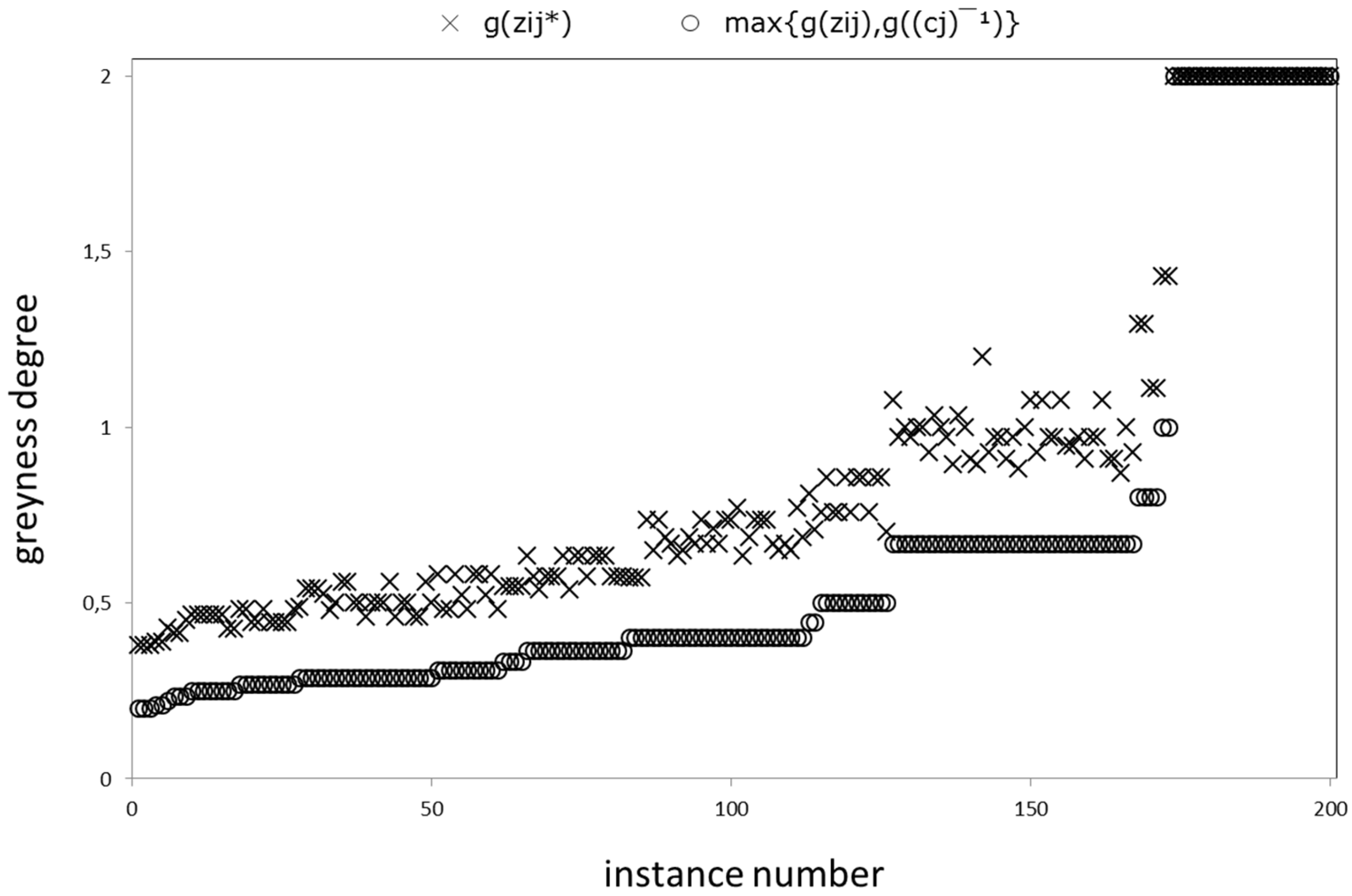
Secondly, we compare the terms of Equation (15). Figure 2 is an illustration of the results for normalization instances following Step 2 of the SAW algorithm. Similarly, note that the maximum series for either the individual greyness degrees or the greyness of the inverses for respective columns is a lower envelope to the greyness degrees of normalization. This verifies our findings in Theorem 5. The stepwise structure that is observable in the lower series is because we use a pre-determined set of discrete linguistic labels at the assessment; as we sort the resultant greyness degree data, inevitably, equal values follow alongside each other.
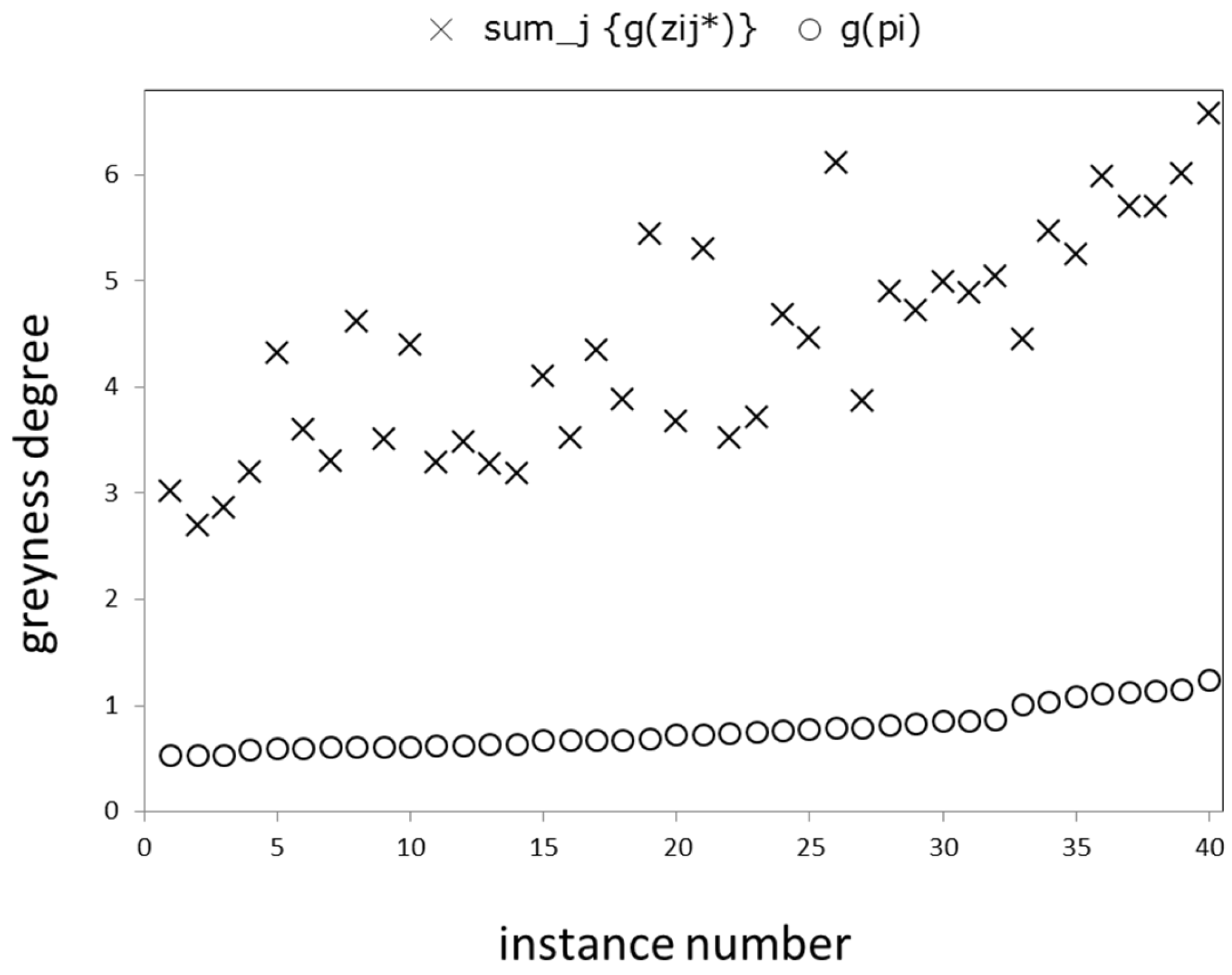
Thirdly, we compare the terms of Equation (10). Figure 3 is a summary of the results for convex combination instances following Step 3 of the SAW algorithm. Expectedly, we recognize that as the sum of individual greyness degrees along each row intensify, the greyness degree series of convex combination for the rows follows with a lower envelope. This verifies our findings in Theorem 3.

7. Illustration of Information Content Results: A Dice-Rolling Experiment

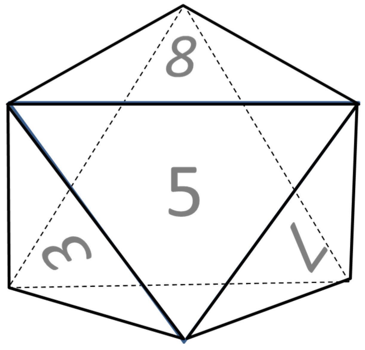
In this section we illustrate our arguments that relate to information content with the aid of a dice-rolling experiment. For this purpose, consider an unusual yet fair 8-faceted die illustrated in Figure 4. In this experiment, the observer rolls the die once, and notes the number that shows up on the top facet of the die.
In this case, obviously we have B = 1 , , 8 . Now suppose that we do not hold our assumption that the grey numbers under study are continuous, and for this section allow discrete representations of grey numbers. Then, consider the following three numbers:
z 1 = 2 , 3 , 4 , 7 , z 2 = 1 , 3 , 4 , 5 , and z 3 = 4 , 5 , 6 , 7 . Let the measure with this background be the probability measure. Clearly, we have m B = 1 .
In order to find the information content of the union of these grey numbers, first we observe z 1 z 2 z 3 = 1 , , 7 , then find the following:
z 1 z 2 z 3 = B z 1 z 2 z 3 = 8 .
We then utilize the following:
I z 1 z 2 z 3 = m z 1 z 2 z 3 m B = 1 / 8 1 = 1 8 .
Now, in order to find this information content result with our arguments, we employ Theorem 6 and just obtain the following:
I i = 1 3 z i = i = 1 3 I z i = 4 / 8 1 · 4 / 8 1 · 4 / 8 1 = 1 8 ,
which shows that Theorem 6 works perfectly.
On the other hand, in order to find the information content of the intersection of these grey numbers, we again observe z 1 z 2 z 3 = 4 , then find the following:
z 1 z 2 z 3 = B z 1 z 2 z 3 = 1 , 2 , 3 , 5 , 6 , 7 , 8 .
Then, similarly we utilize the following:
I z 1 z 2 z 3 = m z 1 z 2 z 3 m B = 7 / 8 1 = 7 8 .
Again, in order to find this information content result with our arguments, we employ Theorem 7 and obtain the following:
I i = 1 3 z i = u 3 I z i
and then see that we need the appropriate set union law:
u 3 I z i = I z 1 + I z 2 + I z 3 I z 1 · I z 2 I z 1 · I z 3 I z 2 · I z 3 + I z 1 · I z 2 · I z 3
Thus, we obtain the following:
u 3 I z i = 4 8 + 4 8 + 4 8 4 8 · 4 8 4 8 · 4 8 4 8 · 4 8 + 4 8 · 4 8 · 4 8 = 7 8 ,
which therefore shows that Theorem 7 works as intended.

8. Conclusions and Future Research Directions

Greyness degree and information content are two unique features with grey numbers, both of which have intrinsic principles and appealing deeds. They are valuable concepts worth inspecting both from an axiomatic and mathematical viewpoint, and from an information science notion. Liu and Lin [12,65] provide an introduction to these concepts and proposed a series of preliminary mathematical results in considering mathematical operations of two grey numbers.
In the current note, we extended their preliminary results by considering opportunities to ponder a sequence of grey numbers in addition to a number of new mathematical operations. To that aim, we developed greyness degree results that relate to summation, conic combination, convex combination, and normalization on a sequence of grey numbers. As an auxiliary result to explore normalization, we also solved for the inverse operation which is associated with a single grey number. In due course, we will give new definitions, such as for conic combination, convex combination, normalization, and union and intersection over a sequence of grey numbers.
We showed that after operations such as summation and conic and convex combination, the total greyness degree observed in a sequence reduces in the final results. We also showed that normalization is the step where greyness degree amplifies during implementation steps of an algorithm under study, such as in the algorithm of the SAW method we examined in this paper.
Furthermore, we developed two results that are useful to calculate information content of union and intersection of a sequence of grey numbers in an uncomplicated manner. The authenticity of our formulae is demonstrated with an interesting example that brings together concepts from set theory and probability theory.
We strongly believe that our results will be useful to researchers who study grey systems, grey prediction, grey decision making, and grey control models, as well as those interested in information theory and information representation.
Could the presented uncertainty representation principles and arguments be applied to solve engineering problems? We strongly believe that this is probable, given the modeling principle of uncertainty under interval representation of grey numbers and the novel use of existing well-grounded methods, such as the Monte Carlo method that we used in this study, which is suitable to simulating probability of occurrence of phenomena.
One such area of application, for example, may be in the stability analysis of underground structures. In this domain, there are important issues regarding the stability of surrounding rock when a structure is built in a specific geological location. Numerical simulations that consider the behavior of the surrounding masses of rock may be studied, where significant parameters such as the rock stress can be modeled under the uncertainty representation. Then, these parameters can be used to forecast possible deformations in the surrounding rock content.
Another closely related engineering problem is to determine the degree of cracking in rock massifs. In this domain, issues that relate to directions and angles of cracks are essential to evaluate the extent of structural disturbance in a massif. However, most of the time, it is very difficult for engineers to obtain a complete/exact set of relevant geomechanical data. In this case, an approach that brings together the capabilities of uncertainty representation principles, which we studied in this paper, and the competence of traditional methods of measurement may provide promising results in unifying a reliable set of input data in order to analyze the degree of cracking in a rock massif.
In the future, we propose that interested researchers should analyze similar operational rules under different representations of grey numbers and compare their results with our findings. Moreover, we propose that researchers should apply the principles of uncertainty representation studied in this paper, and at the same time try to employ traditional methods of their specific domain to solve intricate engineering problems, two of which we analyzed above.

Author Contributions

Conceptualization, İ.G., O.Ç. and B.G.; methodology, İ.G., O.Ç. and B.G.; formal analysis, İ.G., O.Ç. and B.G.; writing—original draft preparation, İ.G., O.Ç. and B.G. All authors have read and agreed to the published version of the manuscript.

Funding

The APC was funded by İstanbul Topkapı University.

Institutional Review Board Statement

Not applicable.

Informed Consent Statement

Not applicable.

Data Availability Statement

Not applicable.

Acknowledgments

The authors (i) acknowledge the careful reading and valuable suggestions provided by all three referees; (ii) thank referee #2 for pointing out interesting probable use cases of our modeling approach, both of which improved the presentation of the paper. The authors acknowledge APC support by İstanbul Topkapı University.

Conflicts of Interest

The authors declare no conflict of interest.

References

  1. Deng, J. Control problems of grey systems. Syst. Control Lett. 1982, 1, 288–294. [Google Scholar]
  2. Deng, J. Grey systems control. J. Huazhong Univ. Sci. Technol. 1982, 3, 9–18. [Google Scholar]
  3. Deng, J. The theory and method of socioeconomic grey systems. Soc. Sci. China 1984, 6, 47–60. [Google Scholar]
  4. Deng, J. Grey Systems: Society, Economy; National Defence Press: Beijing, China, 1985. [Google Scholar]
  5. Deng, J. The Essential Methods of Grey Systems; Huazhong University of Science and Technology Press: Wuhan, China, 1987. [Google Scholar]
  6. Liu, S.; Forrest, J. The mysteries for continual growth of grey system theory. In Proceedings of the 2007 IEEE International Conference on Systems, Man and Cybernetics, Montréal, QC, Canada, 7–10 October 2007; pp. 2155–2159. [Google Scholar]
  7. Li, Q.; Liu, S.; Forrest, J.Y.-L. Fundamental definitions and calculation rules of grey mathematics: A review work. J. Syst. Eng. Electron. 2015, 26, 1254–1267. [Google Scholar] [CrossRef]
  8. Javanmardi, E.; Liu, S.; Xie, N. Exploring grey systems theory-based methods and applications in sustainability studies: A systematic review approach. Sustainability 2020, 12, 4437. [Google Scholar] [CrossRef]
  9. Camelia, D. Grey systems theory in economics–a historical applications review. Grey Syst. Theory Appl. 2015, 5, 263–276. [Google Scholar] [CrossRef]
  10. Islam, R.; Biswal, M.P.; Alam, S.S. Preference programming and inconsistent interval judgments. Eur. J. Oper. Res. 1997, 97, 53–62. [Google Scholar] [CrossRef]
  11. Lee, Y.-M. Development of the grey analytic hierarchy process: A preliminary study. J. Chin. Inst. Environ. Eng. 2002, 12, 175–183. [Google Scholar]
  12. Liu, S. A new definition on degree of greyness of grey numbers with several theorems. In Proceedings of the 2005 IEEE International Conference on Networking, Sensing and Control, Tucson, AZ, USA, 19–22 March 2005; pp. 90–93. [Google Scholar]
  13. Yang, Y. Extended grey numbers and their operations. In Proceedings of the 2007 IEEE International Conference on Systems, Man and Cybernetics, Montréal, QC, Canada, 7–10 October 2007; p. 2181. [Google Scholar]
  14. Despotis, D.K.; Derpanis, D. A min-max goal programming approach to priority derivation in AHP with interval judgments. Int. J. Inf. Technol. Decis. Mak. 2007, 10, 21. [Google Scholar]
  15. Jiang, C.; Han, X.; Guan, F.J.; Li, Y.H. An uncertain structural optimization method based on nonlinear interval number programming and interval analysis method. Eng. Struct. 2007, 29, 3168–3177. [Google Scholar] [CrossRef]
  16. Çakır, O. Post-optimality analysis of priority vectors derived from interval comparison matrices by lexicographic goal programming. Appl. Math. Comput. 2008, 204, 261–268. [Google Scholar]
  17. Yang, Y.; Liu, S. Kernels of grey numbers and their operations. In Proceedings of the 2008 IEEE International Conference on Fuzzy Systems, Hong Kong, China, 1–6 June 2008; 826-831. [Google Scholar]
  18. Jiang, C.; Han, X.; Liu, G.P. Uncertain optimization of composite laminated plates using a nonlinear interval number programming method. Comput. Struct. 2008, 86, 1696–1703. [Google Scholar] [CrossRef]
  19. Çakır, O. The grey extent analysis. Kybernetes 2008, 37, 997–1015. [Google Scholar] [CrossRef]
  20. Zhang, H.; Zhang, W.; Mei, C. Entropy of interval-valued fuzzy sets based on distance and its relationship with similarity measure. Knowl.-Based Syst. 2009, 22, 449–454. [Google Scholar] [CrossRef]
  21. Sun, Y.; Huang, G.H.; Li, Y.P.; Xu, Y.; Cao, M.F. An interval fuzzy robust nonlinear program for the planning of municipal solid waste management systems under uncertainty. Eng. Optim. 2009, 41, 989–1016. [Google Scholar] [CrossRef]
  22. Wu, C.; Huang, G.; Yan, X.; Cai, Y.; Li, Y.; Lv, N. An inexact optimization model for evacuation planning. Kybernetes 2009, 38, 1676–1683. [Google Scholar] [CrossRef]
  23. Salmeron, J.L. Modelling grey uncertainty with fuzzy grey cognitive maps. Expert Syst. Appl. 2010, 37, 7581–7588. [Google Scholar] [CrossRef]
  24. Suprajitno, H.; Mohd, I.B. Linear programming with interval arithmetic. Int. J. Contemp. Math. Sci. 2010, 5, 323–332. [Google Scholar]
  25. Xie, N.-M.; Liu, S. Novel methods on comparing grey numbers. Appl. Math. Model. 2010, 34, 415–423. [Google Scholar] [CrossRef]
  26. Guo, R.; Guo, D.; Cui, Y.H. An uncertain regression model. Grey Syst. Theory Appl. 2011, 1, 202–215. [Google Scholar] [CrossRef]
  27. Liu, S.; Xie, N.-M.; Forrest, J. Novel models of grey relational analysis based on visual angle of similarity and nearness. Grey Syst. Theory Appl. 2011, 1, 8–18. [Google Scholar] [CrossRef]
  28. Yang, Y.; Liu, S. Reliability of operations of grey numbers using kernels. Grey Syst. Theory Appl. 2011, 1, 57–71. [Google Scholar] [CrossRef]
  29. Çakır, O. A compensatory model for computing with words under discrete labels and incomplete information. Knowl.-Based Syst. 2012, 27, 29–37. [Google Scholar] [CrossRef]
  30. Wang, Z. Evaluation of the teachers’ occupation ability based on grey system theory. In Proceedings of the IEEE 9th International Conference on Fuzzy Systems and Knowledge Discovery, Sichuan, China, 29–31 May 2012; pp. 565–568. [Google Scholar]
  31. Wang, J.; Liu, S. Efficiency measures in DEA with grey interval data under the hypotheses of data consistency. Grey Syst. Theory Appl. 2012, 2, 63–69. [Google Scholar] [CrossRef]
  32. Ruan, A.; Fang, Z. Grey potential degrees and its application in grey game. J. Grey Syst. 2013, 25, 19–35. [Google Scholar]
  33. Çakır, O. On visualizing the number comparison scheme in grey extent analysis. Kybernetes 2013, 42, 94–105. [Google Scholar] [CrossRef]
  34. Allahdadi, M. New comparison of interval numbers. Int. J. Appl. Math. 2014, 27, 567–571. [Google Scholar]
  35. Li, Q.X.; Lin, Y. A briefing to grey systems theory. J. Syst. Sci. Inf. 2014, 2, 178–192. [Google Scholar]
  36. Liu, Y.; Forrest, J.; Xie, N. Ranking grey numbers based on dominance grey degrees. J. Syst. Eng. Electron. 2014, 25, 618–626. [Google Scholar] [CrossRef]
  37. Bhattacharyya, R. A grey theory based multiple attribute approach for R&D project portfolio selection. Fuzzy Inf. Eng. 2015, 7, 211–225. [Google Scholar]
  38. Zakeri, S.; Keramati, M.A. Systematic combination of fuzzy and grey numbers for supplier selection problem. Grey Syst. Theory Appl. 2015, 5, 313–343. [Google Scholar] [CrossRef]
  39. Yan, S.; Liu, S.; Liu, J.; Wu, L. Dynamic grey target decision making method with grey numbers based on existing state and future development trend of alternatives. J. Intell. Fuzzy Syst. 2015, 28, 2159–2168. [Google Scholar] [CrossRef]
  40. Nasseri, S.H.; Yazdani, A.; Darvishi, D. A primal simplex algorithm for solving linear programming problem with grey cost coefficients. J. New Res. Math. 2016, 1, 121–141. [Google Scholar]
  41. Ye, Y.; Yao, N.; Wang, Q.; Wang, Q. A method of ranking interval numbers based on degrees for multiple attribute decision making. J. Intell. Fuzzy Syst. 2016, 30, 211–221. [Google Scholar] [CrossRef]
  42. Yan, S.; Liu, S.; Liu, X. Dynamic grey target decision making method with three-parameter grey numbers. Grey Syst. Theory Appl. 2016, 6, 169–179. [Google Scholar] [CrossRef]
  43. Guo, S.; Liu, S.; Fang, Z. Algorithm rules of interval grey numbers based on different kernel and the degree of greyness of grey numbers. Grey Syst. Theory Appl. 2017, 7, 168–178. [Google Scholar] [CrossRef]
  44. Nasseri, S.H.; Darvishi, D.; Yazdani, A. A new approach for solving grey assignment problems. Control Optim. Appl. Math. 2017, 2, 15–28. [Google Scholar]
  45. Stanujkic, D.; Zavadskas, E.K.; Liu, S.; Karabasevic, D.; Popovic, G. Improved OCRA method based on the use of interval grey numbers. J. Grey Syst. 2017, 29, 49–60. [Google Scholar]
  46. Darvishi, D.; Liu, S.; Nasseri, S.H. A new approach in animal diet by grey system theory. Grey Syst. Theory Appl. 2018, 8, 167–180. [Google Scholar]
  47. Li, P.; Wei, C. A new two-stage grey evaluation decision-making method for interval grey numbers. Kybernetes 2018, 47, 801–815. [Google Scholar] [CrossRef]
  48. Mahmoudi, A.; Feylizadeh, M.R. A grey mathematical model for crashing of projects by considering time, cost, quality, risk and law of diminishing returns. Grey Syst. Theory Appl. 2018, 8, 272–294. [Google Scholar] [CrossRef]
  49. Darvishi, D.; Forrest, J.; Liu, S. A comparative analysis of grey ranking approaches. Grey Syst. Theory Appl. 2019, 9, 472–487. [Google Scholar] [CrossRef]
  50. Javed, S.A.; Liu, S.; Mahmoudi, A.; Nawaz, M. Patients’ satisfaction and public and private sectors’ health care service quality in Pakistan: Application of grey decision analysis approaches. Int. J. Health Plan. Manag. 2019, 34, 168–182. [Google Scholar] [CrossRef] [PubMed]
  51. Mahmoudi, A.; Liu, S.; Javed, S.A.; Abbasi, M. A novel method for solving linear programming with grey parameters. J. Intell. Fuzzy Syst. 2019, 36, 161–172. [Google Scholar] [CrossRef]
  52. Chen, N.; Xie, N. Uncertainty representation and information measurement of grey numbers. Grey Syst. Theory Appl. 2020, 10, 495–512. [Google Scholar] [CrossRef]
  53. Ye, J.; Dang, Y.; Yang, Y. Forecasting the multifactorial interval grey number sequences using grey relational model and GM (1, N) model based on effective information transformation. Soft Comput. 2020, 24, 5255–5269. [Google Scholar] [CrossRef]
  54. Ulutaş, A.; Popovic, G.; Stanujkic, D.; Karabasevic, D.; Zavadskas, E.K.; Turskis, Z. A new hybrid MCDM model for personnel selection based on a novel grey PIPRECIA and grey OCRA methods. Mathematics 2020, 8, 1698. [Google Scholar] [CrossRef]
  55. Esangbedo, M.O.; Bai, S.; Mirjalili, S.; Wang, Z. Evaluation of human resource information systems using grey ordinal pairwise comparison MCDM methods. Expert Syst. Appl. 2021, 182, 115151. [Google Scholar] [CrossRef]
  56. Mahmoudi, A.; Deng, X.; Javed, S.A.; Zhang, N. Sustainable supplier selection in megaprojects: Grey ordinal priority approach. Bus. Strateg. Environ. 2021, 30, 318–339. [Google Scholar] [CrossRef]
  57. Stanujkić, D.; Karabašević, D.; Popović, G.; Stanimirović, P.S.; Saračević, M.; Smarandache, F.; Katsikis, V.N.; Ulutaş, A. A new grey approach for using SWARA and PIPRECIA methods in a group decision-making environment. Mathematics 2021, 9, 1554. [Google Scholar] [CrossRef]
  58. Toan, P.N.; Dang, T.-T.; Hong, L.T.T. E-learning platform assessment and selection using two-stage multi-criteria decision-making approach with grey theory: A case study in Vietnam. Mathematics 2021, 9, 3136. [Google Scholar] [CrossRef]
  59. Zanon, L.G.; Marcelloni, F.; Gerolamo, M.C.; Carpinetti, L.C.R. Exploring the relations between supply chain performance and organizational culture: A fuzzy grey group decision model. Int. J. Prod. Econ. 2021, 233, 108023. [Google Scholar] [CrossRef]
  60. Wu, W. A revised grey relational analysis method for multicriteria group decision-making with expected utility theory for oil spill emergency management. Math. Probl. Eng. 2021, 2021, 6682332. [Google Scholar] [CrossRef]
  61. Xiong, P.; Chen, S.; Yan, S. Time-delay nonlinear model based on interval grey number and its application. J. Syst. Eng. Electron. 2022, 33, 370–380. [Google Scholar] [CrossRef]
  62. Wang, L.; Liu, J. Dynamic uncertainty quantification and risk prediction based on the grey mathematics and outcrossing theory. Appl. Sci. 2022, 12, 5389. [Google Scholar] [CrossRef]
  63. Gürler, İ.; Çakır, O.; Gündüzyeli, B. Distance-based decision making, consensus building, and preference aggregation systems: A note on the scale constraints. Systems 2022, 10, 112. [Google Scholar] [CrossRef]
  64. Liu, S.; Fang, Z.; Forrest, J. On algorithm rules of interval grey numbers based on the ‘kernel’ and the degree of greyness of grey numbers. In Proceedings of the 2010 IEEE International Conference on Systems, Man and Cybernetics, İstanbul, Turkey, 10–13 October 2010; pp. 756–760. [Google Scholar]
  65. Liu, S.; Lin, Y. Grey Information. Theory and Practical Applications; Springer: London, UK, 2006. [Google Scholar]
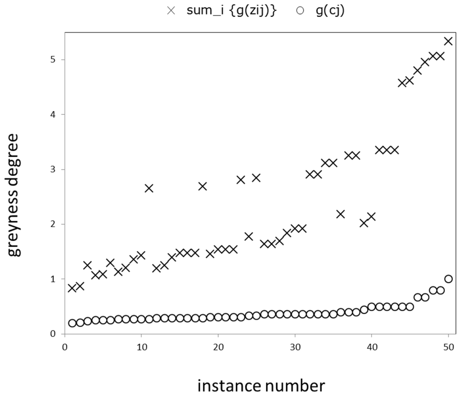
Figure 1. Greyness degree results for summation.
Axioms 11 00424 g001
Figure 2. Greyness degree results for normalization.
Axioms 11 00424 g002
Figure 3. Greyness degree results for convex combination.
Axioms 11 00424 g003
Figure 4. An 8-faceted die.
Axioms 11 00424 g004
Table 1. Summary of subject literature on grey systems.
Source FeaturesMethods and TheoriesCases and Illustrations
[10]Inconsistent grey judgmentsLexicographic goal programmingNumerical examples
[11]Grey decision makingPreference programmingProject selection
[12]Greyness degreeTheorem provingProofs
[13]Extended grey numbersGrey number operationsNumerical examples
[14]Grey decision makingGoal programmingNumerical example
[15]Uncertain structural optimizationNonlinear programmingOptimization of an automobile frame
[16]Post-optimality analysisLexicographic goal programmingNumerical examples
[17]Kernels of grey numbersGrey number operationsNumerical examples
[18]Nonlinear grey programmingHybrid algorithmsOptimization of composite laminated plate
[19]Grey extent analysisProbability theorySupplier selection
[20]Entropy of grey numbersSimilarity measureNumerical example
[21]Grey robust programNonlinear programmingMunicipal solid waste management
[22]Grey linear programModel decompositionEvacuation planning
[23]Grey cognitive mapCognitive mappingAnalyzing IT project risk
[24]Grey linear programmingModified simplex methodNumerical example
[25]Grey number comparisonProbability theoryNumerical examples
[26]Uncertain regressionMultivariate analysisPrediction model examples
[27]Similarity and nearnessGrey relational analysisNumerical example
[28]Kernels of grey numbersGrey number operationsNumerical examples
[29]Discrete linguistic labelsCompensatory programmingBudget allocation
[30]Grey target decision making Grey relational analysisEvaluation of occupational ability
[31]Data consistencyData envelopment analysisNumerical example
[32]Grey potential degreeGame theoryNumerical examples
[33]Visualization Probability theoryNumerical examples
[34]Grey number comparisonPartial ordersProofs
[35]Grey information axioms Grey number operationsProofs
[36]Dominance grey degreeRanking Numerical example
[37]Linguistic labelsGrey possibility degreeR&D project evaluation
[38]Linguistic labelsGrey relational analysisSupplier selection
[39]Dynamic grey targetGrey relational analysisNumerical example
[40]Grey linear programPrimal simplex algorithmNumerical example
[41]Visualization RankingNumerical example
[42]Grey target decision making Dynamic decision makingNumerical example
[43]Greyness degreeRankingNumerical example
[44]Grey linear assignment Hungarian algorithmNumerical example
[45]Operational competitiveness ratingRankingNumerical examples
[46]Diet problem Grey linear programmingAnimal nutrition case
[47]Clustering of grey numbersPossibility definitionNumerical example
[48]Project managementSensitivity analysisNumerical example
[49]Comparative analysisOrder relationsNumerical example
[50]Empirical dataGrey relational analysisHealthcare sector case
[51]Staged solution procedureGrey linear programmingComparative analysis
[52]Probability function of a grey numberInformation representationNumerical example
[53]Information transformationGrey predictionTraffic congestion analysis
[54]Multiple-criteria decision makingGrey arithmeticProduction manager selection
[55]Multiple-criteria decision makingGrey arithmeticComparative analysis
[56]Ordinal priority Membership functionsSupplier selection
[57]Group decision makingGrey arithmeticEvaluating travel websites
[58]Multiple-criteria decision makingHybrid grey decision modelE-learning platform assessment
[59]Group decision makingGrey clusteringTwo case studies
[60]Expected utilitiesGrey relational analysisEmergency management
[61]Time-delay grey modelPossibility theorySimulation
[62]Uncertainty quantificationPossibility indexSafety prediction of laminated plates
[63]Consensus buildingDistance-metric optimizationCase study, computational experiment
Table 2. Linguistic label set for assessments.
Linguistic LabelUnderlying Grey NumberTest Number Interval
Unsatisfactory performance 0 ,   3 / 2 0.0000–0.1666
Poor performance 3 / 2 ,   3 0.1667–0.3333
Mediocre performance 3 ,   9 / 2 0.3334–0.5000
Acceptable performance 9 / 2 ,   6 0.5001–0.6667
Good performance 6 ,   15 / 2 0.6668–0.8334
Exceptional performance 15 / 2 ,   9 0.8335–1.0000
Table 3. Test instances.
InstanceUnderlying SAW StepNumbers of Instances
SummationStep 150
NormalizationStep 2200
Convex combinationStep 340
Publisher’s Note: MDPI stays neutral with regard to jurisdictional claims in published maps and institutional affiliations.