1. Introduction
We developed a set of curves for the gasification of municipal solid waste [
1] using symbolic regression [
2]. The curves were tested statistically, and among those with satisfactory results in terms of Mean Square Error (MSE) and Pearson Correlation Coefficient (PCC) some are not acceptable because they show unexpected oscillatory behavior. To eliminate them, we applied dynamic system criteria by measuring complexity using approximate and sample entropy where the inappropriate curves can be eliminated to persist Occam’s Razor [
3]. We prefer not to present more statistical metrics aside MSE and PCC because they cannot measure behavior between the testing points (on the other hand, dynamic system criteria can).
Gasification of municipal solid waste and biomass gives the different compositions of the synthetic gas (syngas) depending on the gasification temperature in the process [
4]. Based on real measurements of a plasma gasifier, a symbolic model for an important component of the produced syngas is constructed where the percentage in the mixture is given depending on the gasification temperature. To construct these symbolic syngas composition models, the artificial intelligence provided outcomes using symbolic regression software tools AI Feynman [
5] and PySR [
6]. The candidate symbolic models were chosen among those with better statistical metrics; those with a lower Mean Square Error (MSE) and with the Pearson Correlation Coefficient (PCC) close to one. However, it was discovered that some of the obtained symbolic models, which fit very well the measured gasification datasets using statistical metrics, are of oscillatory nature, which was not expected and does not reflect the true physical properties of the modelled gasification process. However, using dynamic system criteria in addition to statistical metrics, such suspicious symbolic models that do fit well the measured gasification datasets were automatically detected and abandoned. This communication will show the universal method based on dynamic system criteria which can detect suitable models among all those which has good properties following statistical metrics. The dynamic system criteria measure the complexity of the candidate models using approximate and sample entropy. Our results indicate that candidate symbolic regression models with oscillations and other non-physical phenomena have higher complexity and can be automatically detected and excluded by approximate and sample entropy to persist Occam’s Razor “science always prefers the simpler model or representation of two which give similar accuracy” [
6]. Consequently, we propose that the dynamic system criteria based on approximate or sample entropy should be used for the automated evaluation of symbolic regression models, as it is not enough to evaluate the models by statistical metrics.
2. Gasification Models
Gasification models were developed for the production of hydrogen (H2) and carbon dioxide (CO2) from municipal solid waste for only six different temperatures, while the measurements were repeated four times.
These functions were introduced in symbolic regression software to provide numerically stable logarithm-based functions, which are defined for all real numbers. As logarithms are defined only for positive non-zero numbers, logarithms pose numerical problems in the symbolic regression procedure, when the argument is negative.
Mean Square Error (MSE) and with the Pearson Correlation Coefficient (PCC) were calculated using functions of Python 3.9 by:
where “data” means the measured data set and “y_pred” means the predicted values using the selected symbolic regression model.
MSE and corr.coef were calculated for all measured data.
The presented models in Matlab notifications are given in
Appendix A to this Communication.
2.1. Hydrogen H2
The train set for hydrogen
H2 is given in
Table 1 while three test sets are given in
Table 2.
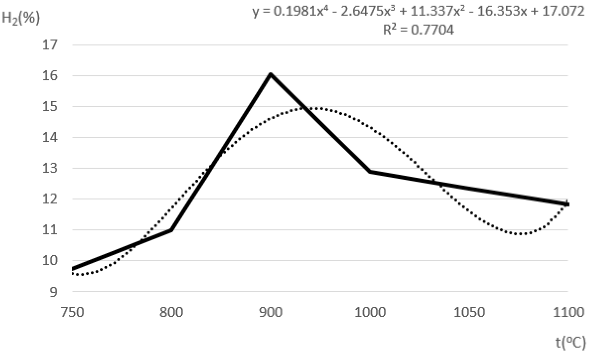
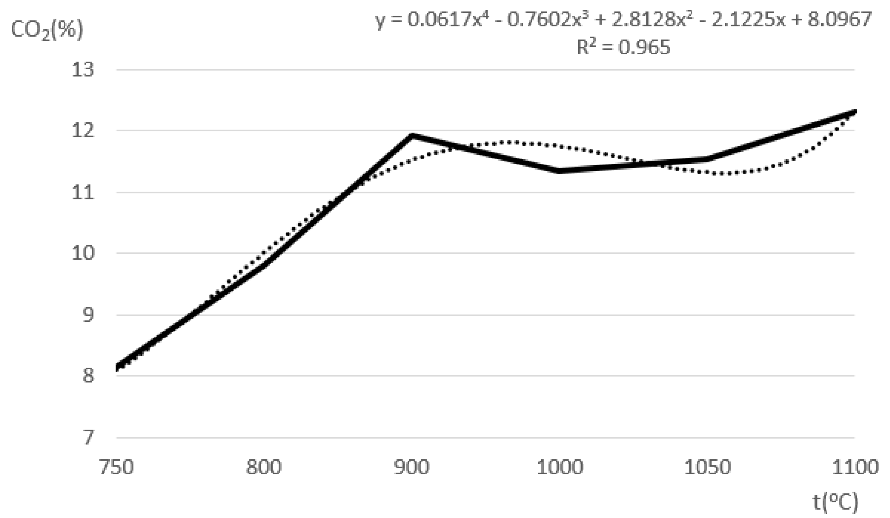
The expected shape of the modelled curves for hydrogen
H2 is given in
Figure 1 where the trendline is based on data from
Table 1 and was produced in MS Excel as a polynomial curve of order 4.
Using symbolic regression tools, three different models were produced as follows.
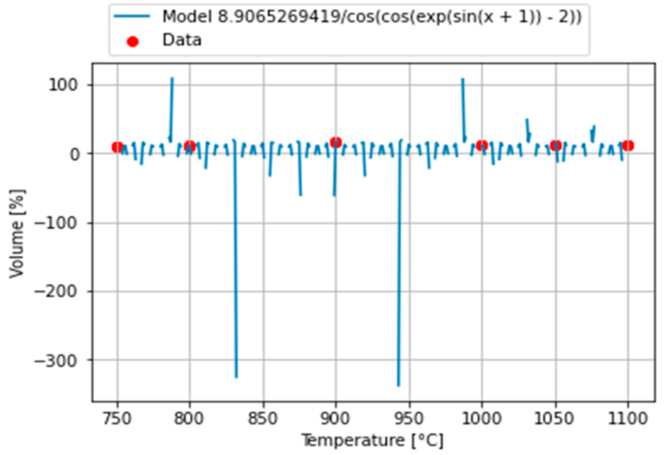
2.1.1. Model 1 of Hydrogen H2
The first developed model is given in Equation (1)
This model performs good statistical metrics; MSE = 0.2897 and PCC = 0.9728 while anyway, it shows oscillatory tendencies as can be seen in
Figure 2.
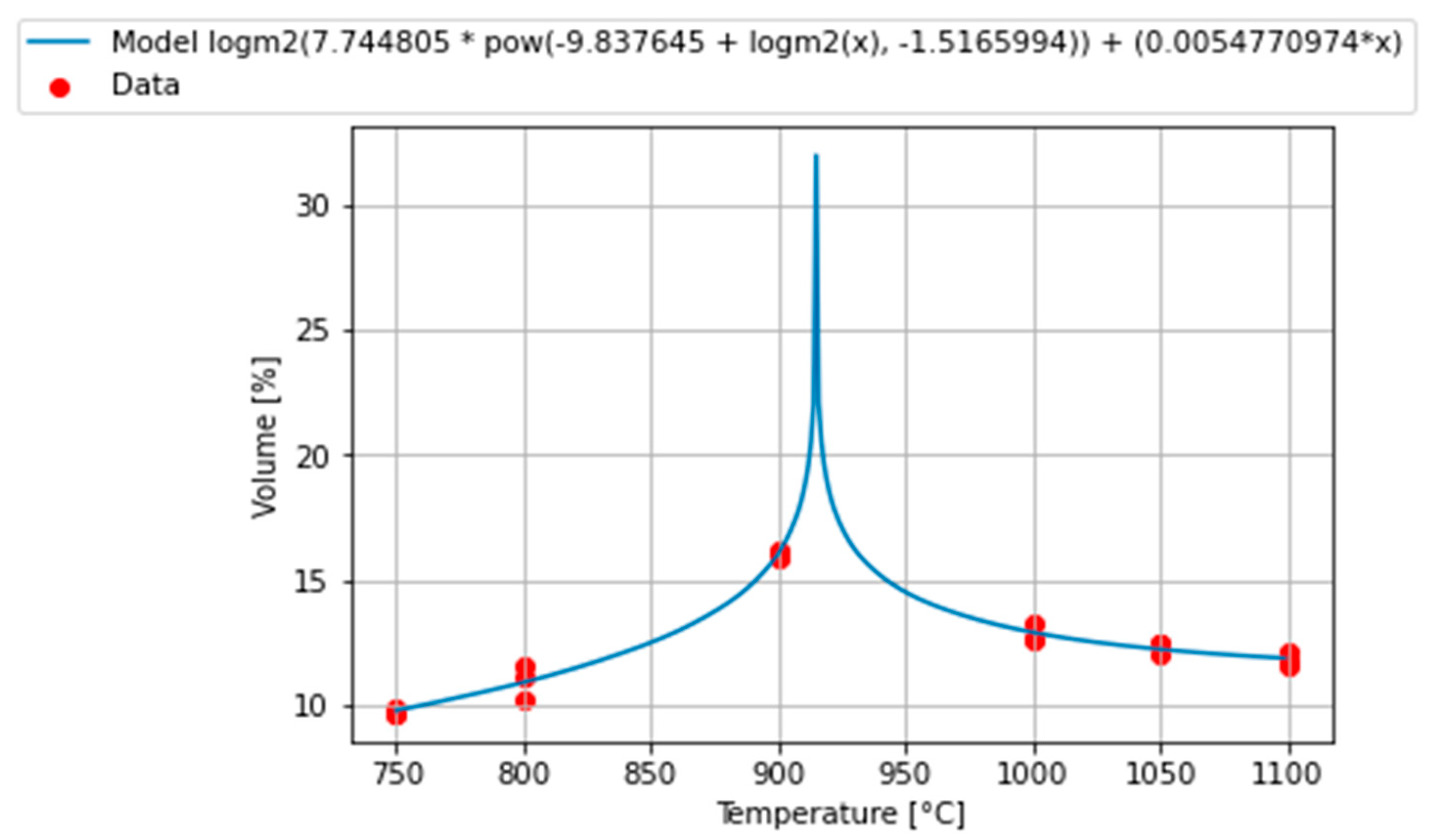
2.1.2. Model 2 of Hydrogen H2
The second developed model is given in Equation (2)
This model performs good, as indicated by statistical metrics, MSE = 0.08143851 and PCC = 0.989470395. Model 2 has improved shape compared with Model 1, despite the undesired tendency towards a sharp peak. It is given in
Figure 3.
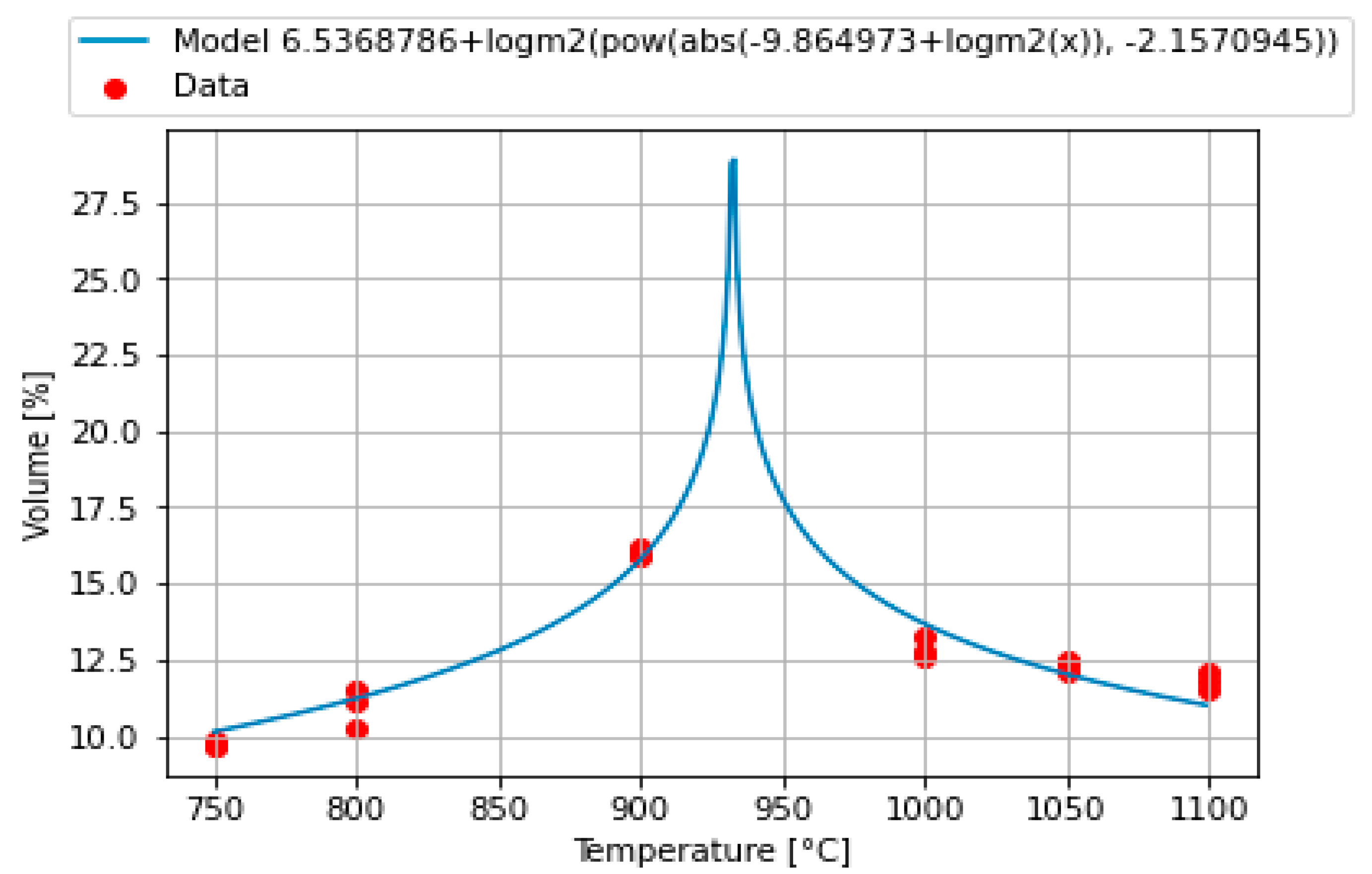
2.1.3. Model 3 of Hydrogen H2
The second developed model is given in Equation (3)
This model performs good statistical metrics, MSE = 0.362862372 and PCC = 0.952248777. It shows the same tendency as Model 2. Model 3 is given in
Figure 4.
2.2. Hydrogen CO2
The train set for hydrogen CO
2 is given in
Table 3 while three test sets are given in
Table 4.
The expected shape of the modelled curves for hydrogen CO
2 is given in
Figure 5 where the trendline is based on data from
Table 3 and was produced in MS Excel as a polynomial curve of order 4.
Using the symbolic regression tools, three different models were produced as follows.
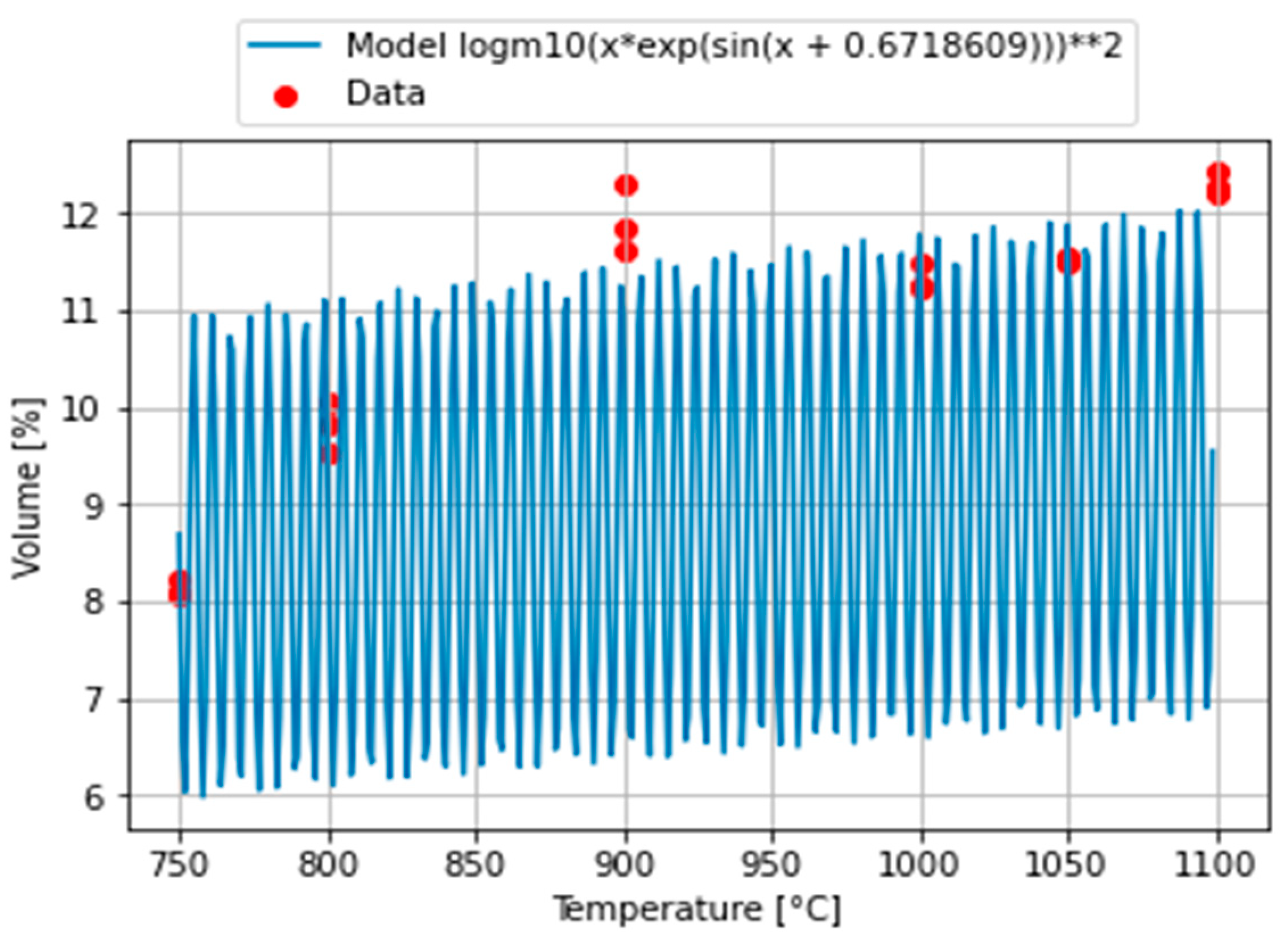
2.2.1. Model 1 of Carbon Dioxide CO2
The first developed model is given in Equation (4)
This model performs good statistical metrics, MSE = 0.3481 and PCC = 0.9171, while it shows oscillatory tendencies, as can be seen in
Figure 6.
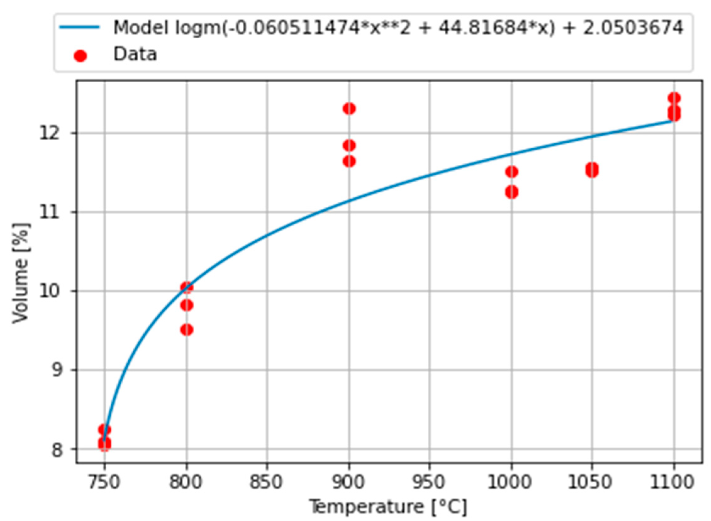
2.2.2. Model 2 of Carbon Dioxide CO2
The first developed model is given in Equation (5)
This model performs good statistical metrics, MSE = 0.1985 and PCC = 0.9519, with a good shape of the developed curve, as can be seen in
Figure 7.
3. Dynamic System Criteria for Selection of Appropriate Models
As observed, it is possible to construct many different models of the investigated phenomena having comparable precision. Now, the task is to select one of them that can be signed as the best choice under the assumption of Occam’s Razor [
3]. For this purpose, the qualification tools from the area of dynamical systems, like approximate
and sample
entropy [
7,
8,
9,
10,
11], can be applied.
Hence, the selection process, based on observation of the measure of complexity, works as follows. Firstly, construct models (e.g., as in the previous section). Secondly, measure the complexity of each model and order them with respect to this measure (in our case approximate and sample entropy). Finally, pick the model with the smallest complexity value (at this stage the assumption of Occam’s Razor [
3] is applied). Here, note that since the minimum need not be unique the output of this selection process will always exist, but should not be unique in general as we will show in the next section.
3.1. Entropy Notions
Approximate entropy
and sample entropy
are tools of complexity measurement that were investigated by many authors and applied in numerous research fields (e.g., [
12,
13,
14]) to measure and compare studied cases’ complexity.
3.1.1. Approximate Entropy Eapp
Recall these notions are defined for the input vector
of length
. Approximate entropy
is defined in Equation (6)
where
and
is the number of
such that
, divided by
. Here,
is an element of
-dimensional real space,
are test parameters and
is the maximum metric. For these parameters holds:
is the length of the window,
is the diameter of the region with a similar subsequence.
3.1.2. Sample Entropy Esamp
On the other hand, sample entropy
is given in Equation (7)
where
is the number of template vector pairs such that
, and
is the number of template vector pairs such
. Here,
is the Chebyshev distance and parameters
have the same meaning as in the case of
.
3.2. Benchmark Models Application
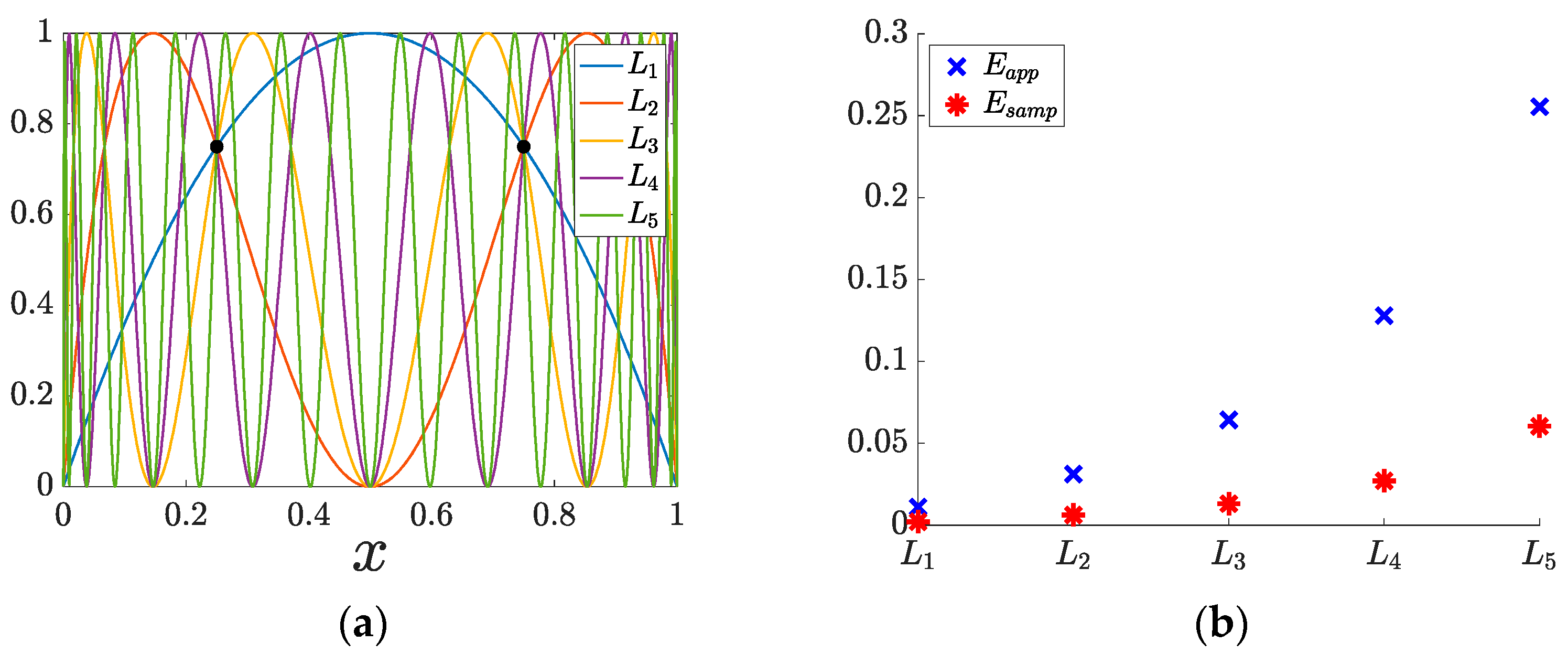
To depict previously mentioned complexity measurement tools, classical models from the theory of dynamical systems can be applied. The well-known logistic function can be used as example of normalized models (also can be thought as predictive one). Recall
and
, this model is well understood from dynamical point of view [
15]. The next model can be constructed as a second iteration of
that is
, and analogously
,
,
. The evolution of these models is shown in
Figure 8a and their corresponding entropies are in
Figure 8b, clearly showing increase of entropy while the complexity of the model increases.
3.3. Simulation Outputs
The numerical simulations of our models were performed in Matlab while the continuous models were discretized from 750 °C to 1100 °C by the step of 0.001 °C. Entropies tests were set classically, that is,
was picked as 20% of the standard deviation of the investigated vector and
was set to 1 as the minimum window length. Firstly, note that the test performed on all models coincides so, for simplicity, we can use the abbreviation of entropy for both tests. These outputs, rounded on four decimal places, are summarized in
Table 5 for hydrogen
H2 and in
Table 6 for carbon dioxide CO
2.
Model 1 of
H2 (which is periodic with a period of 6.283183 °C) has higher complexity than Model 2 of
H2 and Model 3 of
H2, so Model 1 of
H2 can be denied. It is also observable from
Table 5 that entropies of Model 2 of
H2 and Model 3 of
H2 are comparable and much less than Model 1 of
H2.
It is observable from
Table 6 that entropy of the Model 1 of CO
2 is much higher than that of Model 2 of CO
2, proving that Model 2 has lower complexity than Model 1 and is then a better choice.
4. Conclusions
We developed symbolic regression models for the gasification of municipal solid waste [
16,
17,
18,
19,
20,
21]. However, these models were developed using limited points of data and so, between these points, it shows unpredicted behavior (sharp picks or oscillatory motions) where all such models were acceptable using statistic metrics (Mean Square Error and the Pearson Correlation Coefficient) as criteria. In the end, the proposed application of approximate
and sample
entropy automatically detected those models with higher complexity contradicting Occam’s Razor assumption. Hence, the models with higher complexity can be excluded from further investigation. Moreover, it is possible to use these dynamic tools automatically in general for decision mechanisms. The example is about gasification of waste, but the shown method for rejection of inappropriate models is of general value and can be used in various scientific fields. It is based on dynamic system criteria and it is based on the measurement of entropy. In future, we would like to also test Symbolic Functional Evolutionary Search (SyFES), that automatically constructs accurate functionals in the symbolic form, which is more explainable to humans, cheaper to evaluate, and easier to integrate into existing software codes [
22].
However, the proposed selection method is based on approximate and sample entropy, there are also other tools in the mathematical theory of dynamical systems that can be applied [
23,
24]. For example, metrics from recurrence quantification analysis (RQA) can be applied (or relevant alternatives mentioned in [
25]). We propose these promising tools for further research.
In the end, since the proposed method is addressed in general to any set of models it can be also applied to prediction models. The application of the method to the prediction models is left for future research.
Author Contributions
Conceptualization, P.P., M.L., R.P. and D.B.; methodology, P.P., M.L. and R.P.; software, R.P., M.L. and P.P.; validation, P.P., M.L., J.N. and R.P.; formal analysis, P.P., T.K. and M.L.; investigation, P.P. and M.L.; resources, T.K.; data curation, J.N.; writing—original draft preparation, M.L. and D.B.; writing—review and editing, D.B., P.P. and T.K.; visualization, R.P., M.L. and D.B.; supervision, T.K. and P.P.; project administration, P.P. and J.N.; funding acquisition, P.P., T.K., J.N. and M.L. All authors have read and agreed to the published version of the manuscript.
Funding
This work was supported by the Ministry of Education, Youth and Sports of the Czech Republic through the e-INFRA CZ (ID:90140), by the Technology Agency of the Czech Republic through the project “Center of Energy and Environmental Technologies” TK03020027 and by VSB—Technical University of Ostrava, Czech Republic through the Grant of SGS No. SP2022/42.
Informed Consent Statement
Not applicable.
Data Availability Statement
All data to repeat computations are given in the text.
Conflicts of Interest
The authors declare no conflict of interest.
Appendix A
The models in Matlab notifications are:
H2 models:
= 8.9065269419/cos(cos(exp(sin(x + 1)) − 2))
= logm2(7.744805 * pow(-9.837645 + logm2(x), −1.5165994)) + (0.0054770974*x)
= 6.5368786+logm2(pow(abs(−9.864973 + logm2(x)), −2.1570945))
CO2 models:
= logm10(x.*exp(sin(x + 0.6718609))).^2
= logm(−0.060511474*x.^2+44.81684*x) + 2.0503674
pow = @(x,y) x.^y
logm = @(x) log(abs(x) + 1e-8);
logm2 =@(x) log2(abs(x) + 1e-8);
logm10 = @(x) log10(abs(x) + 1e-8)
References
- Praks, P.; Brkić, D.; Najser, J.; Najser, T.; Praksová, R.; Stajić, Z. Methods of Artificial Intelligence for Simulation of Gasification of Biomass and Communal Waste. In Proceedings of the 22nd International Carpathian Control Conference (ICCC), Velké Karlovice, Czech Republic, 31 May–1 June 2021. [Google Scholar] [CrossRef]
- Praks, P.; Brkić, D. Symbolic Regression-Based Genetic Approximations of the Colebrook Equation for Flow Friction. Water 2018, 10, 1175. [Google Scholar] [CrossRef]
- Dresp-Langley, B.; Ekseth, O.K.; Fesl, J.; Gohshi, S.; Kurz, M.; Sehring, H.-W. Occam’s Razor for Big Data? On Detecting Quality in Large Unstructured Datasets. Appl. Sci. 2019, 9, 3065. [Google Scholar] [CrossRef]
- Baláš, M.; Lisý, M.; Štelcl, O. The Effect of Temperature on the Gasification Process. Acta Polytech. 2012, 52, 7–11. Available online: http://hdl.handle.net/10467/66949 (accessed on 10 July 2022). [CrossRef]
- Udrescu, S.-M.; Tegmark, M. AI Feynman: A physics-inspired method for symbolic regression. Sci. Adv. 2020, 6, eaay2631. [Google Scholar] [CrossRef]
- Cranmer, M.; Sanchez-Gonzalez, A.; Battaglia, P.; Xu, R.; Cranmer, K.; Spergel, D.; Ho, S. Discovering symbolic models from deep learning with inductive biases. Adv. Neural Inf. Process. Syst. 2020, 33, 17429–17442. Available online: https://proceedings.neurips.cc/paper/2020/file/c9f2f917078bd2db12f23c3b413d9cba-Paper.pdf (accessed on 8 July 2022).
- Pincus, S.M. Approximate entropy as a measure of system complexity. Proc. Natl. Acad. Sci. USA 1991, 88, 2297–2301. [Google Scholar] [CrossRef]
- Chon, K.H.; Scully, C.G.; Lu, S. Approximate entropy for all signals. IEEE Eng. Med. Biol. Mag. 2009, 28, 18–23. [Google Scholar] [CrossRef]
- Delgado-Bonal, A.; Marshak, A. Approximate Entropy and Sample Entropy: A Comprehensive Tutorial. Entropy 2019, 21, 541. [Google Scholar] [CrossRef]
- Richman, J.S.; Moorman, J.R. Physiological time-series analysis using approximate entropy and sample entropy. Am. J. Physiol. Heart Circ. Physiol. 2000, 278, H2039–H2049. [Google Scholar] [CrossRef]
- Yentes, J.M.; Hunt, N.; Schmid, K.K.; Kaipust, J.P.; McGrath, D.; Stergiou, N. The appropriate use of approximate entropy and sample entropy with short data sets. Ann. Biomed. Eng. 2013, 41, 349–365. [Google Scholar] [CrossRef]
- Buchlovská Nagyová, J.; Jansík, B.; Lampart, M. Detection of embedded dynamics in the Györgyi-Field model. Sci. Rep. 2000, 10, 21031. [Google Scholar] [CrossRef]
- Lampart, M.; Vantuch, T.; Zelinka, I.; Mišák, S. Dynamical properties of partial-discharge patterns. Int. J. Parallel Emergent Distrib. Syst. 2018, 33, 474–489. [Google Scholar] [CrossRef]
- Lampart, M.; Zapoměl, J. Motion of an Unbalanced Impact Body Colliding with a Moving Belt. Mathematics 2021, 9, 1071. [Google Scholar] [CrossRef]
- Lampart, M.; Martinovič, T. A survey of tools detecting the dynamical properties of one-dimensional families. Adv. Electr. Electron. Eng. 2017, 15, 304–313. [Google Scholar] [CrossRef]
- Akkaya, E.; Demir, A. Energy content estimation of municipal solid waste by multiple regression analysis. In Proceedings of the 5th International Advanced Technologies Symposium IATS’09, Karabuk, Turkey, 13–15 May 2009; pp. 13–15. Available online: https://www.academia.edu/download/54979427/IATS09_03-99_1292.pdf (accessed on 10 July 2022).
- Liu, J.-I.; Paode, R.D.; Holsen, T.M. Modeling the energy content of municipal solid waste using multiple regression analysis. J. Air Waste Manag. Assoc. 1996, 46, 650–656. [Google Scholar] [CrossRef]
- Chu, C.; Boré, A.; Liu, X.W.; Cui, J.C.; Wang, P.; Liu, X.; Chen, G.Y.; Liu, B.; Ma, W.C.; Lou, Z.Y.; et al. Modeling the impact of some independent parameters on the syngas characteristics during plasma gasification of municipal solid waste using artificial neural network and stepwise linear regression methods. Renew. Sustain. Energy Rev. 2022, 157, 112052. [Google Scholar] [CrossRef]
- Malaťáková, J.; Jankovský, M.; Malaťák, J.; Velebil, J.; Tamelová, B.; Gendek, A.; Aniszewska, M. Evaluation of Small-Scale Gasification for CHP for Wood from Salvage Logging in the Czech Republic. Forests 2021, 12, 1448. [Google Scholar] [CrossRef]
- Lapcik, V.; Lapcikova, M.; Hanslik, A.; Jez, J. Possibilities of gasification and pyrolysis technology in branch of energy recovery from waste. Inżynieria Mineralna 2014, 15, 149–154. Available online: http://potopk.com.pl/Full_text/2014_full/2014_1_19.pdf (accessed on 10 July 2022).
- Kůdela, J.; Smejkalová, V.; Šomplák, R.; Nevrlý, V. Legislation-induced planning of waste processing infrastructure: A case study of the Czech Republic. Renew. Sustain. Energy Rev. 2020, 132, 110058. [Google Scholar] [CrossRef]
- Ma, H.; Narayanaswamy, A.; Riley, P.; Li, L. Evolving symbolic density functionals. Science Advances. Available online: https://doi.org/10.1126/sciadv.abq0279 (accessed on 19 July 2022).
- Kizielewicz, B.; Więckowski, J.; Shekhovtsov, A.; Wątróbski, J.; Depczyński, R.; Sałabun, W. Study towards the time-based MCDA ranking analysis—A supplier selection case study. Facta Univ. Ser. Mech. Eng. 2021, 19, 381–399. [Google Scholar] [CrossRef]
- Bogach, N.; Boitsova, E.; Chernonog, S.; Lamtev, A.; Lesnichaya, M.; Lezhenin, I.; Novopashenny, A.; Svechnikov, R.; Tsikach, D.; Vasiliev, K.; et al. Speech Processing for Language Learning: A Practical Approach to Computer-Assisted Pronunciation Teaching. Electronics 2021, 10, 235. [Google Scholar] [CrossRef]
- Kantz, H.; Schreiber, T. Nonlinear Time Series Analysis, 2nd ed.; Cambridge University Press: Cambridge, UK, 2003. [Google Scholar] [CrossRef]
| Publisher’s Note: MDPI stays neutral with regard to jurisdictional claims in published maps and institutional affiliations. |
© 2022 by the authors. Licensee MDPI, Basel, Switzerland. This article is an open access article distributed under the terms and conditions of the Creative Commons Attribution (CC BY) license (https://creativecommons.org/licenses/by/4.0/).


 ,
, 


