Article

Sharp Power Mean Bounds for Two Seiffert-like Means †

1
Department of Science and Technology, Stated Grid Zhejiang Electric Power Company Research Institute, Hangzhou 310014, China
2
Institute of Fundamental and Interdisciplinary Sciences, Beijing Union University, Beijing 100101, China
*
Author to whom correspondence should be addressed.
Both authors humbly dedicate this paper to our cherished friend, Professor Shi Huannan, as he approaches his 75th birthday.
Axioms 2023, 12(10), 910; https://doi.org/10.3390/axioms12100910
Submission received: 6 August 2023 / Revised: 29 August 2023 / Accepted: 4 September 2023 / Published: 25 September 2023

Abstract

:
The mean is a subject of extensive study among scholars, and the pursuit of optimal power mean bounds is a highly active field. This article begins with a concise overview of recent advancements in this area, focusing specifically on Seiffert-like means. We establish sharp power mean bounds for two Seiffert-like means, including the introduction and establishment of the best asymmetric mean bounds for symmetric means. Additionally, we explore the practical applications of these findings by extending several intriguing chains of inequalities that involve more than ten means. This comprehensive analysis provides a deeper understanding of the relationships and properties of these means.
MSC:
26E60; 26D05; 26A48

1. Introduction

In the realm of mathematical inequalities, the concept of mean, in its various manifestations, holds a distinguished place. Mean, whether it be arithmetic, geometric, or one of its many counterparts, has been a steadfast companion to mathematicians throughout history. Its roots extend back to the earliest mathematical writings, where thinkers grappled with the notions of balance and fairness. From ancient civilizations to the luminaries of the Enlightenment, the concept of mean has played a pivotal role in shaping the discourse of mathematics.
As we embark on the journey of sharing our findings and insights, we do so with a profound reverence for the rich mathematical heritage and literature that have guided us to this juncture. Our objective is to weave a new thread into the intricate tapestry of inequalities, one that pays homage to the historical significance of mean while pushing the boundaries of mathematical knowledge.
The symmetrical beauty inherent in mathematical inequalities resonates with the aesthetics of a finely crafted masterpiece. It is as though mean serves as a mathematical brushstroke, imbuing the canvas of equations and proofs with an artistic touch.
In our pursuit, we are akin to intrepid explorers navigating uncharted territory, and we celebrate mean as our guiding compass through the labyrinth of mathematical inequalities. We acknowledge its role not only as a scientific cornerstone but also as an artistic element that enriches our mathematical journey.
Throughout the paper, we consider the condition that a , b > 0 with a b . For r R , the power mean of order r of the positive real numbers a and b is defined by
A r A r a , b = a r + b r 2 1 / r if r 0 and A 0 A 0 a , b = a b ,
which has the following properties:
(i) The function r A r a , b is continuous and increasing on R (see [1]), and is log-concave on 0 , and log-convex on ( , 0 ) (see [2]).
(ii) The function r 2 1 / r A r a , b is strictly decreasing and log-convex on 0 , (Lemma 6 [3]).
More generally, the power mean of order r of a and b with weight w 0 , 1 is defined by
A r a , b ; w = w a r + 1 w b r 1 / r if r 0 and A 0 a , b ; w = a w b 1 w ,
which satisfies that r A r a , b ; w is increasing on R for fixed w 0 , 1 .
As special cases, we have A = A a , b = A 1 a , b , G = G a , b = A 0 a , b , H = H a , b = A 1 a , b , which are the arithmetic mean, geometric mean and harmonic mean, respectively.
Various symmetric and homogeneous bivariate means exist, including the Heronian mean H e ( a , b ) , the logarithmic mean L ( a , b ) and the identric (exponential) mean I ( a , b ) , which are defined by
H e a , b = a + b + a b 3 , L a , b = a b ln a ln b , I a , b = e 1 a a b b 1 / ( a b ) ,
respectively. The three means have sharp lower and upper bounds in terms of power means, namely,
A ln 2 / ln 3 a , b < H e a , b < A 2 / 3 a , b ,
A 0 a , b < L a , b < A 1 / 3 a , b ,
A 2 / 3 a , b < I a , b < A ln 2 a , b ,
where all orders of these power means in the above three double inequalities are the best possible. The inequalities (2), (3), and (4) are derived from references [4], [5], and [6,7], respectively.
There are also three bivariate means of the same form, which are the first Seiffert mean P ( a , b ) [8], the second Seiffert mean T ( a , b )  [9] and Neuman–Sándor mean N S a , b [10], which are defined by
P a , b = a b 2 arcsin a b a + b , T a , b = a b 2 arctan a b a + b , N S a , b = a b 2 arsinh a b a + b ,
respectively. The three means also have the best power mean bounds, which are
A ln 2 / ln π a , b < P a , b < A 2 / 3 a , b ,
A ln 2 / ( ln π ln 2 ) a , b < T a , b < A 5 / 3 a , b ,
A ln 2 / [ ln ( ln ( 3 + 2 2 ) ) ] a , b < N S ( a , b ) < A 4 / 3 ( a , b ) .
The inequalities (6), (7), and (8) are derived from references [11,12,13], [14,15], and [3,15,16], respectively.
Moreover, Yang [17] introduced two new means defined by
U a , b = a b 2 arctan a b 2 a b and V a , b = a b 2 arsinh a b 2 a b ,
which also have the sharp lower and upper power mean bounds:
A ln 4 / 2 ln π ln 2 a , b < U a , b < A 4 / 3 a , b ,
A 0 a , b < V a , b < A 2 / 3 a , b .
The inequalities (9) and (10) are derived from references [18] and [19], respectively.
Other bivariate means and the best bounds for them can be seen in the following articles:
(i) Gauss arithmetic–geometric mean [20];
(ii) Toader mean [21] and the best power mean bounds were established in [22], Corollary (1) [23], Theorem 22 [24];
(iii) Toader–Qi mean, see Theorem 3.4 [25];
(iv) Sándor mean, see [26,27];
(v) Sándor–Yang mean, see [17,28].
In particular, it is worth mentioning that, inspired by the first and second Seiffert means, Witkowski [29] introduced the Seiffert-like mean defined by
M f a , b = a b 2 f a b a + b ,
where f is defined on 0 , 1 satisfying
t 1 + t < f t < t 1 t ,
and is called the Seiffert functions. Clearly, the Seiffert functions have two important properties:
lim t 0 f 0 = 0 and lim t 0 f t t = 1 .
Letting f = arcsin , arctan , arsinh , artanh in (11) produces the first and second Seiffert means, Nueman–Sándor mean, and logarithmic mean. Taking f = sinh , tan in (11) gives
M sinh a , b = a b 2 sinh a b a + b ,
M tan a , b = a b 2 tan a b a + b ,
which are called the hyperbolic sine mean and tangent mean of a and b, respectively. Recently, the two new means, namely M sinh a , b and M tan a , b , caught the attention of some scholars, and several bounds for the two new means have been established. Witkowski [29] presented a chain of comparison inequalities among the Seiffert-like means L, P, M tan , M sinh , and A:
L < P M tan < M sinh < A ,
where the means in the curly brackets are not comparable. In 2020, Nowicka and Witkowski [30] provided the optimal weighted power mean bounds A p ( A , G ; w ) ( p = ± 1 , ± 2 ) for the two new means M sinh and M tan . In another paper [31], the authors established the best weighted power mean bounds A p ( A , H ; w ) ( p = ± 1 , ± 2 ) for M sinh and M tan , which were generalized by Zhu [32], Zhu and Malešević [33] as follows: the double inequalities
2 3 A q + 1 3 H q 1 / q < M tan < 2 3 A p + 1 3 H p 1 / p , 5 6 A s + 1 6 H s 1 / s < M sinh < 5 6 A r + 1 6 H r 1 / r ,
hold for p ln ( 3 / 2 ) / ln tan 1 , q 4 / 5 and r 32 / 25 , s ln ( 6 / 5 ) / ln sinh 1 .
Other types of bounds for the two new means M sinh and M tan can be seen in [34,35,36].
From the published literature, however, there seems to be a gap in the research on power mean bounds for the two new means. The aim of this paper is to find the best power mean bounds for them. Our main results read as follows:
Theorem 1. 
The double inequality
A p a , b < M sinh a , b < A q a , b
holds if and only if p 2 / 3 and q p 1 = ln 2 / ln 2 + ln sinh 1 = 0.811
Theorem 2. 
Let p , q > 0 and α p = 1 2 sinh 1 p . If b > a > 0 , then the double inequality
A p a , b ; α p < M sinh a , b < A q a , b ; α q
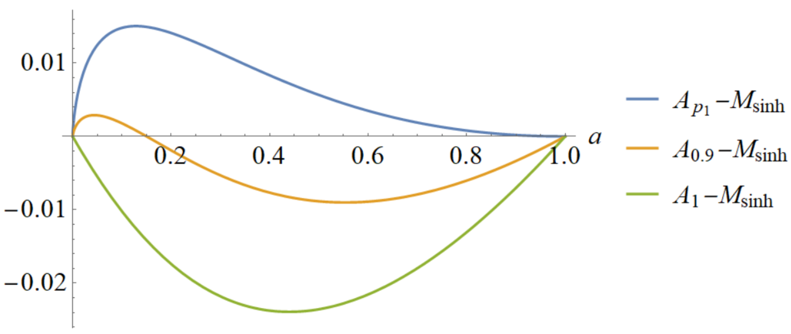
holds if and only if p 1 and 0 < q p 1 = ln 2 / ln 2 + ln sinh 1 = 0.811 Refer to Figure 1 and Figure 2. Moreover, p A p a , b ; α p is decreasing on 0 , .
Theorem 3. 
The double inequality
A p a , b < M tan a , b < A q a , b
holds if and only if p 1 / 3 and q p 0 = ln 2 / ln 2 + ln tan 1 = 0.610
Theorem 4. 
Let p , q > 0 and β p = 1 2 tan 1 p . If b > a > 0 , then the double inequality
A p a , b ; β p < M tan a , b < A q a , b ; β q
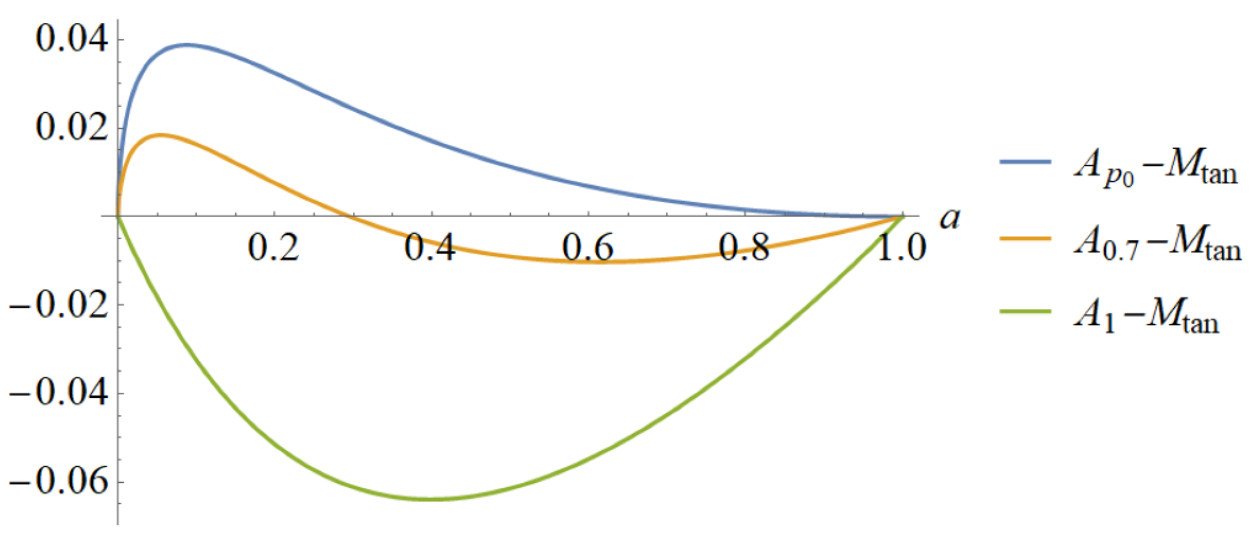
holds if and only if p 1 and 0 < q p 0 = ln 2 / ln 2 + ln tan 1 = 0.610 Refer to Figure 3 and Figure 4. Moreover, p A p a , b ; β p is decreasing on 0 , .
The organization of the remaining sections of this paper is structured as follows. In Section 2, four tools and three monotonicity results are listed, which are needed to prove our main results. Proofs of Theorems 1–4 are presented in Section 3. In the fourth section, several chains of inequalities for means including eight old means and two new Seiffert-like means are established.

2. Preliminaries

2.1. Tools

Several tools are required for establishing our main results. The first tool is the so-called L’Hospital monotonic rule (LMR).
Proposition 1 
(Theorem 2 [37]). Let < a < b < , and let f , g : [ a , b ] R be continuous functions that are differentiable on a , b , with f a = g a = 0 or f b = g b = 0 . Assume that g ( x ) 0 for each x in ( a , b ) . If f / g is increasing (decreasing) on ( a , b ) then so is f / g .
To introduce the second tool, we introduce an important auxiliary function H f , g , which appeared in [38] and was called Yang’s H–function in [39]. For a < b , let f and g be differentiable on ( a , b ) and g 0 on ( a , b ) . Then the function H f , g is defined by
H f , g = f g g f .
If f and g are twice differentiable on ( a , b ) , then
f g = g g 2 f g g f = g g 2 H f , g ,
H f , g = f g g .
The following proposition was proved in [38] and is called the L’Hospital piece monotonic rule (LPMR).
Proposition 2. 
Let a < b . Let f and g be differentiable functions on ( a , b ) and let H f , g be defined by (19). Suppose that (i) g 0 on ( a , b ) ; (ii) f ( b ) = g ( b ) = 0 ; (iii) there is a c a , b such that f / g is increasing (respectively, decreasing) on a , c and decreasing (respectively, increasing) on c , b . Then, we have the following:
(i) When g > 0 and H f , g a + 0 r e s p e c t i v e l y , 0 , or g < 0 and H f , g a + 0 r e s p e c t i v e l y , 0 , f / g is decreasing (respectively, increasing) on a , b ;
(ii) When g > 0 and H f , g a + > 0 r e s p e c t i v e l y , < 0 , or g < 0 and H f , g a + < 0 r e s p e c t i v e l y , > 0 , there is a unique number x b a , b such that f / g is increasing (respectively, decreasing) on a , x b and decreasing (respectively, increasing) on x b , b .
A significant role in addressing the monotonicity of power series ratios is played by the third tool, which involves the monotonicity rule for the ratio of two power series as discussed in [40].
Proposition 3. 
Let A t = n = 0 a n t n and B t = n = 0 b n t n be two real power series converging on r , r ( r > 0 ) with b n > 0 for all n. If the sequence { a n / b n } n 0  is increasing (decreasing), then so is the ratio A t / B t on 0 , r .
The fourth tool, established in Theorem 2.1 [41] by Yang, Chu, and Wang, provides a fresh monotonicity rule for power series ratios when the sequence { a n / b n } n 0 is initially increasing (respectively, decreasing), then decreasing (respectively, increasing). The following proposition appeared in [42], which is a slightly modified version of Theorem 2.1 [41].
Proposition 4. 
Let f t = k = 0 a k t k and g t = k = 0 b k t k be two real power series converging on r , r and b k > 0 for all k. Suppose that for certain m N , the sequences a k / b k 0 k m and a k / b k k m are both non-constant, and they are increasing (respectively, decreasing) and decreasing (respectively, increasing), respectively. Then the function f / g is strictly increasing (respectively, decreasing) on 0 , r if and only if H f , g r 0 r e s p e c t i v e l y , 0 . If H f , g r < 0 r e s p e c t i v e l y , > 0 , then there exists t 0 0 , r such that the function f / g is strictly increasing (respectively, decreasing) on 0 , t 0 and strictly decreasing (respectively, increasing) on t 0 , r .
Propositions 3 and 4 are very efficient to study for certain special functions, see for example [43,44,45,46,47,48,49,50,51,52].

2.2. Three Monotonicity Results

The following two monotonicity results are crucial to prove Theorems 5 and 6.
Lemma 1. 
The function
ϕ sinh t = t 1 t 2 2 t cosh 2 t 2 cosh t + t sinh t sinh t sinh t t 1 t cosh t sinh t t t + 1 cosh t
is decreasing from 0 , 1 onto 0 , 1 / 3 .
Lemma 2. 
The function
ϕ tan t = 2 t 1 t 2 sin t t cos t cos t t 2 t + sin t cos t t 2 + t sin t cos t
is decreasing from 0 , 1 onto 0 , 2 / 3 .
We first prove Lemma 1.
Proof of Lemma 1. 
Let
g 1 t = t 1 t 2 2 t cosh 2 t 2 cosh t + t sinh t sinh t , g 2 t = sinh t t 1 t cosh t sinh t t t + 1 cosh t .
Then ϕ sinh t = g 1 t / g 2 t . Using the product-to-sum formula and expanding in power series yield
2 g 1 t = t 2 1 t 2 cosh 2 t 2 t sinh 2 t + 3 t 2 = t 2 1 n = 1 2 2 n 2 2 n 2 ! t 2 n n = 1 2 2 n 2 n 1 ! t 2 n + 3 t 2 = t 2 1 n = 2 2 n 5 2 2 n 2 2 n 1 ! t 2 n = n = 3 2 n 7 2 2 n 4 2 n 3 ! t 2 n n = 2 2 n 5 2 2 n 2 2 n 1 ! t 2 n = n = 3 2 n 2 2 n 1 2 n 7 2 2 n 4 2 n 3 ! 2 n 2 2 n 1 t 2 n n = 3 2 n 5 2 2 n 2 2 n 1 ! t 2 n 2 2 3 ! t 4 = n = 3 n 1 2 n 1 2 n 7 2 2 n 3 2 2 n 5 2 2 n 3 2 n 1 ! t 2 n + 2 3 t 4 = n = 2 a n t 2 n ,
where
a 2 = 2 3 and a n = 2 n 3 2 n 2 7 n 1 2 2 n 3 2 n 1 ! for n 3 ;
2 g 2 t = t 4 cosh 2 t t 2 cosh 2 t cosh 2 t + 2 t sinh 2 t + t 4 t 2 + 1 = n = 2 2 2 n 4 2 n 4 ! t 2 n n = 1 2 2 n 2 2 n 2 ! t 2 n n = 0 2 2 n 2 n ! t 2 n + n = 1 2 2 n 2 n 1 ! t 2 n + t 4 t 2 + 1 = 2 t 4 + n = 3 2 n 1 2 n 3 5 n 2 + n + 4 2 2 n 2 2 n ! t 2 n = n = 2 b n t 2 n ,
where
b 2 = 2 and b n = 2 n 1 2 n 3 5 n 2 + n + 4 2 2 n 2 2 n ! for n 3 .
Obviously, b n > 0 for n 2 . To use Proposition 4, we have to observe the monotonicity of the sequence a n / b n n 2 . A direct verification gives
a 2 b 2 = 1 3 and a n b n = n 2 n 3 2 n 2 7 n 1 2 n 1 2 n 3 5 n 2 + n + 4 for n 3 ,
and then,
d 2 = a 3 b 3 a 2 b 2 = 9 20 1 3 = 47 60 < 0 ,
d n = a n + 1 b n + 1 a n b n = 8 4 n 6 n 4 20 n 3 + 6 n 2 + 6 n 3 2 n 1 2 n + 1 2 n 3 + n 2 3 n + 2 2 n 3 5 n 2 + n + 4 > 0
for n 3 . This shows that the sequence a n / b n n 2 is decreasing for n = 2 , 3 and increasing for n 3 . If we show that H g 1 , g 2 1 < 0 , then by Proposition 4, we deduce that ϕ sinh = g 1 / g 2 is decreasing on 0 , 1 . A direct computation yields
g 1 1 = 0 and g 2 1 = 2 cosh 1 sinh 1 sinh 1 > 0 .
Differentiation leads to
g 1 t = 3 t 2 1 2 t cosh 2 t 2 cosh t + t sinh t sinh t t 1 t 2 2 t cosh t 3 sinh t sinh t , g 2 t = 2 t cosh t + t 2 t sinh t sinh t t t + 1 cosh t + sinh t t 1 t cosh t 2 t cosh t + t t + 1 sinh t ,
which yields
g 1 1 = cosh 2 2 sinh 2 + 3 = 0.491 < 0 , g 2 1 = 3 cosh 2 + 1 > 0 .
We then obtain
H g 1 , g 2 1 = g 1 1 g 2 1 g 2 1 g 1 1 < 0 .
An easy check gives lim t 0 ϕ sinh 0 = 1 / 3 and ϕ sinh 1 = 0 , thereby completing the proof. □
For proving Lemma 2, we need the following lemmas.
Lemma 3. 
For | t | < π , we have
1 sin t = 1 t + n = 1 2 2 n 2 2 n ! B 2 n t 2 n 1 ,
cos t sin t = 1 t n = 1 2 2 n 2 n ! B 2 n t 2 n 1
1 sin 2 t = 1 t 2 + n = 1 2 n 1 2 2 n 2 n ! B 2 n t 2 n 2 ,
cos t sin 2 t = 1 t 2 n = 1 2 n 1 2 2 n 2 2 n ! B 2 n t 2 n 2 .
Proof. 
The power series representations (24) and (25) were listed in Equations (4.3.68) and (4.3.70) [53]. The third and fourth power series representations follow from
1 sin 2 t = cos t sin t and cos t sin 2 t = 1 sin t ,
which completes the proof. □
The Bernoulli numbers B n are defined by the exponential generating function
x e x 1 1 + x 2 = n = 2 B n n ! x n x < 2 π .
The function x / e x 1 1 + x / 2 is even on R , B 2 n + 1 = 0 for n N . An analytic expression exists for even orders, B 2 n = ( 1 ) n 1 2 ( 2 n ) ! ( 2 π ) 2 n s = 1 s 2 n = ( 1 ) n 1 2 ( 2 n ) ! ( 2 π ) 2 n ζ ( 2 n ) for n 1 , where ζ ( · ) is the Riemann zeta function. The following lemma was proved in [54] (see also [55]).
Lemma 4. 
For k N , Bernoulli numbers B 2 k satisfy
2 2 k + 2 1 2 2 k 1 π 2 2 k + 1 2 k + 2 < B 2 k B 2 k + 2 < 2 2 k + 1 1 2 2 k 1 1 π 2 2 k + 1 2 k + 2 .
Now, we are able to prove Lemma 2.
Proof of Lemma 2. 
Let
ξ 2 t = 8 t sin t t cos t cos t , η 2 t = 4 t 2 t + sin t cos t t 2 + t sin t cos t .
Then
ϕ tan t = 1 t 2 ξ 2 t η 2 t .
Since sin t t cos t > 0 and cos t > 0 for t 0 , π / 2 , we have
ξ s = 4 s sin s 2 s 2 cos s 2 cos s 2 = 2 s sin s s 2 cos s s 2 > 0
for s 0 , π . Similarly, we have
η s = 1 2 s 2 s + sin s 1 2 s 2 + s sin s = 1 4 s 4 s 2 + 2 s sin s sin 2 s > 0
for s 0 , π due to η 1 s = s 2 / 2 s + sin s > 0 and η 2 s = s 2 / 2 + s sin s > 0 for s 0 , π . In fact, since
η 1 s = 1 sin s > 0 , η 2 s = 1 + sin s > 0
for s 0 , , and η j 0 = η j 0 = 0 for j = 1 , 2 , we immediately get that η 1 s , η 2 s > 0 for s 0 , . Thus, if we prove that s η s / ξ s is increasing on 0 , π , then the function s ξ s / η s is positive and decreasing on 0 , π , and then, so is t ϕ tan t on 0 , 1 .
Now, expanding in power series leads to
η s sin 2 s = s 4 / 4 s 2 + 2 s sin s sin 2 s sin 2 s = 1 4 s 4 sin 2 s s 2 sin 2 s + 2 s sin s 1 = 1 4 s 2 + n = 1 2 n 1 2 2 n 2 2 n ! B 2 n s 2 n + 2 1 + n = 1 2 n 1 2 2 n 2 n ! B 2 n s 2 n + 2 1 + n = 1 2 2 n 2 2 n ! B 2 n s 2 n 1 = n = 1 a n s 2 n ,
where a 1 = 1 / 4 and for n 2 ,
a n = 2 n 2 n 1 2 n 3 2 2 n 4 B 2 n 2 2 n 3 2 2 n + 4 B 2 n 2 n ! ;
ξ s sin 2 s = s 2 s 2 cos s + 2 s sin s sin 2 s = s 2 sin 2 s s 2 cos s sin 2 s + 2 s sin s = 1 + n = 1 2 n 1 2 2 n 2 n ! B 2 n s 2 n 1 n = 1 2 n 1 2 2 n 2 2 n ! B 2 n s 2 n + 2 + n = 1 2 2 2 n 2 2 n ! B 2 n s 2 n = n = 1 2 2 n + 1 4 n 2 2 n ! B 2 n s 2 n : = n = 1 b n s 2 n ,
where
b n = 2 2 n + 1 4 n 2 2 n ! B 2 n .
It is easy to check that b n > 0 for n 1 , a 1 / b 1 = 3 / 2 and for n 2
a n b n = 2 n 2 n 1 2 n 3 2 2 n 4 B 2 n 2 2 n 3 2 2 n + 4 B 2 n 2 2 n + 1 4 n 2 B 2 n = 2 n 2 n 1 2 n 3 2 2 n 4 2 2 n + 1 4 n 2 B 2 n 2 B 2 n 2 n 3 2 2 n + 4 2 2 n + 1 4 n 2 .
Then, a 2 / b 2 = 20 / 11 , a 3 / b 3 = 154 / 57 , and then,
d 1 = a 2 b 2 a 1 b 1 = 7 22 > 0 and d 2 = a 3 b 3 a 2 b 2 = 554 627 > 0 .
We next show that d n = a n + 1 / b n + 1 a n / b n > 0 for n 3 . Using Lemma 4 yields
a n b n < 2 n 2 n 1 2 n 3 2 2 n 4 2 2 n + 1 4 n 2 2 2 n 1 1 2 2 n 3 1 π 2 2 n 2 n 1 2 n 3 2 2 n + 4 2 2 n + 1 4 n 2 ,
a n + 1 b n + 1 = 2 n + 2 2 n + 1 2 n 1 2 2 n 2 2 2 n + 3 4 n 6 B 2 n B 2 n + 2 2 n 1 2 2 n + 2 + 4 2 2 n + 3 4 n 6 > 2 n + 2 2 n + 1 2 n 1 2 2 n 2 2 2 n + 3 4 n 6 2 2 n + 2 1 2 2 n 1 π 2 2 n + 1 2 n + 2 2 n 1 2 2 n + 2 + 4 2 2 n + 3 4 n 6 .
Then,
d n : = a n + 1 b n + 1 a n b n > 2 n 1 2 2 n 2 2 2 n + 3 4 n 6 2 2 n + 2 1 2 2 n 1 π 2 2 n 1 2 2 n + 2 + 4 2 2 n + 3 4 n 6 2 n 3 2 2 n 4 2 2 n + 1 4 n 2 2 2 n 1 1 2 2 n 3 1 π 2 + 2 n 3 2 2 n + 4 2 2 n + 1 4 n 2 = 4 π 2 4 2 8 n c 3 n 2 6 n + c 2 n 2 4 n + c 1 n 2 2 n 128 4 2 2 n 1 2 2 n 8 2 2 n 2 n 1 2 2 n + 2 2 n 3
where
c 3 n = 6 π 2 4 n 2 + 21 π 2 n + 4 π 2 178 , c 2 n = 12 5 π 2 18 n 2 450 + 5 π 2 , c 1 n = 12 16 π 2 n 2 + 416 5 π 2 .
An easy verification yields that c i n > 0 for i = 1 , 2 , 3 and n 3 , and
c 1 n 2 2 n 128 c 1 2 2 4 128 = 16 1176 53 π 2 > 0
for n 2 ; also, using an obvious inequality
2 2 n = 1 + 3 n > 1 + 3 n + 3 2 n n 1 2 = 1 2 9 n 2 3 n + 2 ,
we obtain that
4 π 2 4 2 2 n c 3 n > 4 π 2 4 1 2 9 n 2 3 n + 2 6 π 2 4 n 2 + 21 π 2 n + 4 π 2 178 = 4 π 2 4 n 2 9 π 2 8 n + 54 > 0 for n 3 ,
which leads to 4 π 2 4 2 8 n c 3 n 2 6 n > 0 for n 3 . It then follows that d n > 0 for n 3 . Consequently, the sequence a n / b n n 1 is increasing, and by Lemma 3, so is the function s η s / ξ s on 0 , π . An easy computation yields
lim t 0 ϕ tan t = 2 3 and ϕ tan 1 = 0 ,
which completes the proof. □
Finally, we prove the decreasing property of p A p y , x ; 1 c p , which is needed to prove Theorems 2 and 4.
Lemma 5. 
Let x > y > 0 and c 0 , 1 . The function
p A p y , x ; 1 c p = 1 c p y p + c p x p 1 / p
is decreasing on 0 , with
lim p 0 A p y , x ; 1 c p = x a n d lim p A p y , x ; 1 c p = max c x , y .
Proof. 
Let t = x / y . Then
A p y , x ; 1 c p = y c t p + c p 1 1 / p , t 1 , .
Differentiation yields
ln A p t = t p 1 t p + c p 1 , p ln A p t = c p t p 1 1 c p t p + c p 1 2 ln t ln c c p 1 .
Since c 0 , 1 and t 1 , , we see that there is a t 0 > 1 such that 2 ln A p / p t < 0 for t 1 , t 0 and 2 ln A p / p t > 0 for t t 0 , , where t 0 = exp ln c / c p 1 . This implies that the function t ln A p / p is decreasing on 1 , t 0 and increasing on t 0 , . Note that
ln A p p = 1 p t p ln t c p ln c t p + c p 1 1 p 2 ln t p + c p 1 .
An easy computation yields
lim t 1 + ln A p p = 0 and lim t ln A p p = 0 .
It then follows that
ln A p p < max lim t 1 + ln A p p , lim t ln A p p = 0 ,
which proves the decreasing property of p A p y , x ; 1 c p on 0 , . The required limit values can be derived by the L’Hospital rule. This completes the proof. □

3. Proofs of Main Results

Due to the symmetry and homogeneous of the means M f a , b and A p a , b , we assume that b > a > 0 and let x = a / b 0 , 1 . Then, the desired inequalities are equivalent to
A p x , 1 < M f x , 1 < A q x , 1
for x 0 , 1 , where f = tan , sinh . We prove Theorems 1–4 by considering the monotonicity pattern of the ratio U f x / V x on 0 , 1 , where
U f x = M f p x , 1 1 and V x = x p 1 .
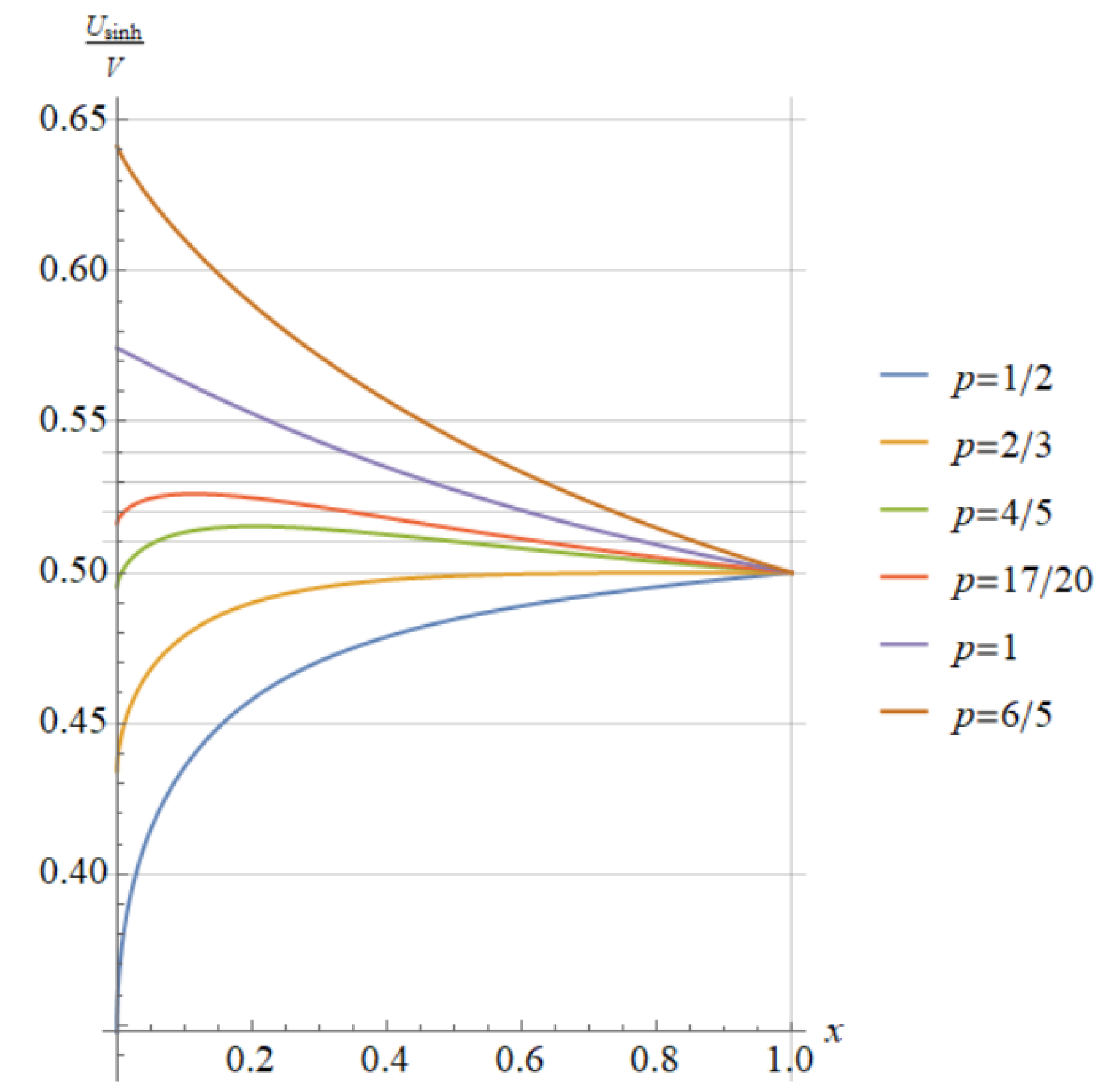
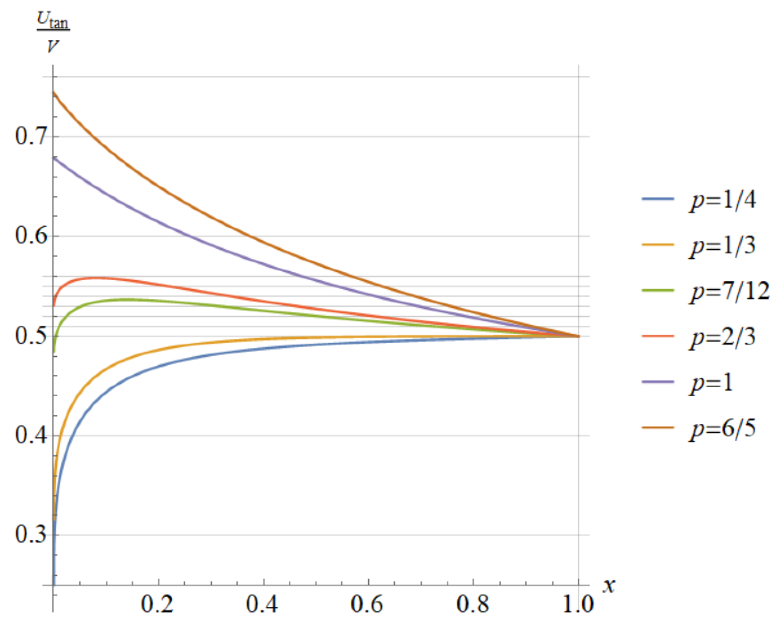
Figure 5 and Figure 6 present the graphs of f = sinh and f = tan of U f x / V x , respectively. We observe the following patterns in the monotonicity of the ratio U f x / V x on 0 , 1 : (i) increase for certain values of p; (ii) decrease for certain values of p; and (iii) increase first and then decrease gradually for certain values of p.
Now, we give a strict proof. Differentiation yields
U f V = p M f p 1 M f p x p 1 = M f p 1 x p 1 M f ,
U f V = p 1 M f x p 2 x M f M f x 2 M f + M f x p 1 M f = M f p 2 x p p 1 x M f M f M f + x M f M f .
Assume that x M f M f M f 0 for x 0 , 1 . Then
U f V = M f p 2 x p x M f M f M f p 1 + x M f M f x M f M f M f .
In order to determine the sign of U f / V on 0 , 1 , we have to find the supremum and infimum of
Φ f x = x M f M f x M f M f M f
on 0 , 1 .
Lemma 6. 
Let f be an odd function on 1 , 1 and third-order differentiable on 0 , 1 . If t 1 ± t f t f t 0 on 0 , 1 , then Φ f x defined by (32) can be expressed as
Φ f x = t 1 t 2 2 f t f t + t f t f t 2 t f t 2 t t 1 f t + f t t t + 1 f t f t = ϕ f t
for t 0 , 1 with
Φ f 0 + = ϕ f 1 = 0 and Φ f 1 = ϕ f 0 + = 1 3 f 0 .
Proof. 
Let t = 1 x / 1 + x . Then x = 1 t / 1 + t and
M f x , 1 = 1 x 2 f 1 x / 1 + x = t 1 + t f t
for t 0 , 1 . Differentiation yields
M f M f x , 1 = d d t t 1 + t f d x d t = 1 + t f t f + t + 1 f 1 + t 2 f 2 t + 1 2 2 = 1 2 t t + 1 f f f 2 ,
M f M f x , 1 = d d t 1 2 t t + 1 f f f 2 d x d t = 1 2 2 t + 1 f + t t + 1 f f f 2 2 f f t t + 1 f f f 4 t + 1 2 2 = 1 4 t + 1 3 2 t f 2 f 2 f + t f f 3 .
Then
x M f M f = 1 t 1 + t 1 2 t t + 1 f f f 2 t 1 + t f = 1 2 t t 2 f f f 2 .
Since f t t 1 ± t f t 0 on 0 , 1 , we see that x M f M f M f 0 for x 0 , 1 . Then
Φ f x = x M f M f x M f M f M f = 1 t 1 + t t 1 + t f 1 4 t + 1 3 2 t f 2 f 2 f + t f f 3 1 2 t t 2 f f f 2 1 2 t t + 1 f f f 2 = t 1 t 2 2 f + t f f 2 t f 2 t t 1 f + f t t + 1 f f .
As shown in (12), f 0 = 0 , f 0 = lim t 0 f t / t = 1 . Moreover, since f is an odd function on 1 , 1 , we easily see that f 0 = 0 . Using the L’Hospital rule gives that, as t 0 ,
t t 1 f t + f t t 2 2 t f t + t t 1 f t 2 t f 0 1 2 f 0 = 1 ,
t 1 + t f t f t t 2 2 t f t + t 1 + t f t 2 t f 0 + 1 2 f 0 = 1 ,
f t 2 f t + t f t 2 t f t 2 t 3 t f t f t 3 f t t f t f t 3 t 2
= 1 3 f t t f t f t t f t f t t 2 1 3 f 0 f 0 f 0 2 = 1 3 f 0 ,
which implies that
Φ f 1 = ϕ f 0 + = 1 3 f 0 .
Due to the differentiability of f on 0 , 1 , f t , f t and f t are bounded on 0 , 1 , and therefore, Φ f 0 + = ϕ f 1 = 0 , which completes the proof. □
Remark 1. 
Under the conditions as Lemma 6, it follows from the limit relations lim t 0 f t / t = 1 and (36) that
lim x 1 M f x , 1 = lim t 0 1 2 t t + 1 f f f 2 = 1 2 lim t 0 t 2 f 2 lim t 0 t t + 1 f f t 2 = 1 2 ,
which implies that
lim x 1 U f x V x = lim x 1 U f x V x = 1 2 .
On the other hand, it is readily seen that
lim x 0 + U f x V x = lim x 0 + M f p x , 1 1 x p 1 = 1 1 2 p f p 1 if p > 0 .

3.1. Proofs of Theorems 1 and 2

We first observe the monotonic pattern of U sinh x / V x on 0 , 1 , which is displayed in the following theorem.
Theorem 5. 
The following statements are valid.
(i) If 0 < p 2 / 3 , the ratio U sinh / V is increasing on 0 , 1 , and therefore, the double inequality
α p < M sinh p x , 1 1 x p 1 < 1 2
holds, where α p = 1 1 / 2 sinh 1 p , or equivalently,
x p + 1 2 1 / p < M sinh x , 1 < α p x p + 1 α p 1 / p
for x 0 , 1 .
(ii) If p 1 , the ratio U sinh / V is decreasing on 0 , 1 , and therefore, the double inequality
1 2 < M sinh p x , 1 1 x p 1 < α p
holds, or equivalently,
α p x p + 1 α p 1 / p < M sinh x , 1 < x p + 1 2 1 / p
for x 0 , 1 .
(iii) If 2 / 3 < p < 1 , there is an x 0 such that the ratio U sinh / V is increasing on 0 , x 0 and decreasing on x 0 , 1 , and therefore, the inequality
min 1 2 , α p M sinh p x , 1 1 x p 1
holds for x 0 , 1 . In particular, when min 1 / 2 , α p = 1 / 2 , that is, ln 2 ln 2 + ln sinh 1 p < 1 , the inequality
M sinh x , 1 < x p + 1 2 1 / p
holds for x 0 , 1 ; when min 1 / 2 , α p = α p , that is, 2 / 3 < p ln 2 ln 2 + ln sinh 1 , the inequality
M sinh x , 1 < α p x p + 1 α p 1 / p
holds for x 0 , 1 .
Proof. 
Let f t = sinh t . Then f t = cosh t and f t = sinh t . By (33)–(35), we see that
M sinh x , 1 = 1 2 t t + 1 cosh t sinh t sinh 2 t , x M sinh x , 1 M sinh x , 1 = 1 2 t t 2 cosh t sinh t sinh 2 t ,
and Φ sinh x = ϕ sinh t , where ϕ sinh t is defined by (22). Clearly, M sinh x , 1 > 0 for x 0 , 1 . Since
t t 2 cosh t sinh t = t 2 cosh t sinh t + t sinh t < 0
for t > 0 , we have that t t 2 cosh t sinh t < 0 for t > 0 , which implies that
x M sinh x , 1 M sinh x , 1 < 0 for x 0 , 1 . Then, by (31), we have that
sgn U sinh x V x = sgn p 1 + Φ sinh x : = sgn μ x .
Lemma 1 tells us that ϕ sinh t is decreasing in t from 0 , 1 onto 0 , 1 / 3 which, by Lemma 6 and x = 1 t / 1 + t , implies that the function Φ sinh x ( = ϕ sinh t ) is increasing in x from 0 , 1 onto 0 , 1 / 3 .
(i) If 0 < p 2 / 3 , then p 1 + Φ sinh x 0 for x 0 , 1 , and so U sinh / V 0 for x 0 , 1 . It follows from Proposition 1 that U sinh / V is increasing on 0 , 1 . This together with (37) and (38) yields
1 1 2 p sinh p 1 = lim x 0 + U sinh x V x < U sinh x V x < lim x 1 U sinh x V x = 1 2
for x 0 , 1 , which implies (39).
(ii) If p 1 , then p 1 + Φ sinh x 0 for x 0 , 1 , and so U sinh / V 0 for x 0 , 1 . It follows from Proposition 1 that U sinh / V is decreasing on 0 , 1 , and therefore, the inequalities
1 2 < U sinh x V x < 1 1 2 p sinh p 1
hold for x 0 , 1 , which implies (40).
(iii) In the case of p 2 / 3 , 1 , since μ x = p 1 + Φ sinh x is increasing on 0 , 1 with μ 0 + = p 1 < 0 and μ 1 = p 2 / 3 > 0 , there is an x 0 0 , 1 such that μ x < 0 for x 0 , x 0 and μ x > 0 for x x 0 , 1 . This, by (44), implies that U sinh / V > 0 for x 0 , x 0 and U sinh / V < 0 for x x 0 , 1 . To use Proposition 2, we also need the signs of V and H U sinh , V 0 + . By (43), it is derived that
M sinh 0 + , 1 = 1 2 lim t 1 t t + 1 cosh t sinh t sinh 2 t = 2 cosh 1 sinh 1 2 sinh 2 1 = 0.691 ,
which together with M sinh 0 + , 1 = 1 / 2 sinh 1 gives
H U sinh , V x = U sinh x V x V x U sinh x = M sinh p 1 x , 1 M sinh x , 1 x p 1 x p 1 M sinh p x , 1 1 1 1 2 sinh 1 p as x 0 + .
Since p 2 / 3 , 1 , we see that H U sinh , V 0 + > 0 . Clearly, V x = p x p 1 > 0 . It then follows from Proposition 2 that there is an x 0 0 , 1 such that U sinh / V is increasing on 0 , x 0 and decreasing on x 0 , 1 , and therefore, we have
min 1 2 , 1 1 2 sinh 1 p U sinh x V x = M sinh p x , 1 1 x p 1
for x 0 , 1 . In particular, when 1 2 sinh 1 p 1 / 2 , that is, ln 2 / ln 2 + ln sinh 1 p < 1 , the inequality (41) holds for x 0 , 1 ; when 1 2 sinh 1 p 1 / 2 , that is, 2 / 3 < p ln 2 / ln 2 + ln sinh 1 , the inequality (42) holds for x 0 , 1 . The proof is thus proved. □
We are now in a position to prove Theorems 1 and 2.
Proof of Theorem 1. 
Assume that b > a > 0 and let x = a / b . Then, the double inequality (15) is equivalent to
x p + 1 2 1 / p < M sinh x , 1 < x q + 1 2 1 / q
for x 0 , 1 . The sufficiency follows from the inequalities (39)–(41) in Theorem 5.
We prove the necessity by the reduction to absurdity. First, we prove that the necessary condition for which the second inequality of (45) holds for x 0 , 1 is q p 1 .
Assume that q 2 / 3 such that the second inequality of (45) holds for x 0 , 1 . By Theorem 5 (i), we have the first inequality of (39) for p = q , which is clearly a contradiction.
Assume that q 2 / 3 , p 1 such that the second inequality of (45) holds for x 0 , 1 . By Theorem 5 (iii), there is an x 0 such that the ratio U sinh / V is increasing on 0 , x 0 and decreasing on x 0 , 1 . Then
1 2 = lim x 1 U sinh x V x < U sinh x V x for x x 0 , 1 ,
that is,
M sinh x , 1 < A q x , 1 for x x 0 , 1 .
On the other hand, q < p 1 implies that α q < 1 / 2 , that is,
α q = lim x 0 + U sinh x V x < lim x 1 U sinh x V x = 1 / 2 .
Then there is an x 1 0 , x 0 such that U sinh x 1 / V x 1 = 1 / 2 . Then
U sinh x V x < U sinh x 1 V x 1 = 1 2 for x 0 , x 1 ,
which implies that
A q x , 1 < M sinh x , 1 for x 0 , x 1 .
These also yield a contradiction. This proves the necessary condition such that the second inequality of (45) holds for x 0 , 1 .
In the same way, we can prove that the necessary condition for which the first inequality of (45) to hold for x 0 , 1 is p 2 / 3 , and the proof is complete. □
Proof of Theorem 2. 
Let x = a / b . Then the double inequality (16) is equivalent to
α p x p + 1 α p 1 / p < M sinh x , 1 < α q x q + 1 α q 1 / q
for x 0 , 1 . The sufficiency follows from the inequalities (40)–(42) in Theorem 5.
The necessity can be proved by the reduction to absurdity. We first prove that the necessary condition such that the second inequality of (46) holds for x 0 , 1 is 0 < q p 1 .
Assume that q 1 such that the second inequality of (46) holds for x 0 , 1 . Then by Theorem 5 (ii), the first inequality of (40) holds for x 0 , 1 and p = q , which yields a contradiction.
Assume that q p 1 , 1 such that the second inequality of (46) holds for x 0 , 1 . By Theorem 5 (iii), there is an x 0 such that the ratio U sinh / V is increasing on 0 , x 0 and decreasing on x 0 , 1 . Then
α q = lim x 0 + U sinh x V x < U sinh x V x for x 0 , x 0 ,
that is,
M sinh x , 1 < A q x , 1 ; α q for x 0 , x 0 .
On the other hand, q > p 1 implies that α q > 1 / 2 , that is,
α q = lim x 0 + U sinh x V x > lim x 1 U sinh x V x = 1 / 2 .
Then there is an x 1 x 0 , 1 such that U sinh x 1 / V x 1 = α q , and therefore,
U sinh x V x < U sinh x 1 V x 1 = α q for x x 1 , 1 ,
which implies that
M sinh x , 1 > A q x , 1 ; α q for x x 1 , 1 .
These yield a contradiction. This proves the necessary condition such that the second inequality of (46) holds for x 0 , 1 .
In a similar way, we can prove that the necessary condition for which the first inequality of (46) to hold for x 0 , 1 is p 1 .
Taking y , x = a , b and c = 1 / 2 sinh 1 in Lemma 5, the decreasing property of p A p a , b ; α p on 0 , follows. This completes the proof. □

3.2. Proofs of Theorems 3 and 4

We begin with observing the monotonic pattern of U tan x / V x on 0 , 1 , which is contained in the following theorem.
Theorem 6. 
The following statements are valid.
(i) If 0 < p 1 / 3 , the ratio U tan / V is increasing on 0 , 1 , and therefore, the double inequality
β p < M tan p x , 1 1 x p 1 < 1 2
holds, where β p = 1 1 / 2 p tan p 1 , or equivalently,
x p + 1 2 1 / p < M tan x , 1 < β p x p + 1 β p 1 / p
for x 0 , 1 .
(ii) If p 1 , the ratio U tan / V is decreasing on 0 , 1 , and therefore, the double inequality
1 2 < M tan p x , 1 1 x p 1 < β p
holds, or equivalently,
β p x p + 1 β p 1 / p < M tan x , 1 < x p + 1 2 1 / p
for x 0 , 1 .
(iii) If 1 / 3 < p < 1 , there is an x 0 such that the ratio U tan / V is increasing on 0 , x 0 and decreasing on x 0 , 1 , and therefore, the inequality
min 1 2 , β p M tan p x , 1 1 x p 1
holds for x 0 , 1 . In particular, when min 1 / 2 , β p = 1 / 2 , that is, ln 2 / ln 2 + ln tan 1 p < 1 , the inequality
M tan x , 1 < x p + 1 2 1 / p
holds for x 0 , 1 ; when min 1 / 2 , β p = β p , that is, 1 / 3 < p ln 2 / ln 2 + ln tan 1 , the inequality
M tan x , 1 < β p x p + 1 β p 1 / p
holds for x 0 , 1 .
Proof. 
Let f t = tan t . Then f t = 1 / cos 2 t and f t = 2 sin t / cos 3 t . By (33)–(35), we see that
M tan x , 1 = 1 2 t 2 + t sin t cos t sin 2 t > 0 , x M tan x , 1 M tan x , 1 = 1 2 t 2 t + cos t sin t sin 2 t < 0 ,
and Φ tan x = ϕ tan t , where ϕ tan t is defined by (23). As shown in the proof of Lemma 2, η 1 s = s 2 / 2 s + sin s > 0 and η 2 s = s 2 / 2 + s sin s > 0 for s 0 , π , which indicate that
M tan x , 1 > 0 and x M tan x , 1 M tan x , 1 < 0
for x 0 , 1 . Then, by (31), we have that
sgn U tan x V x = sgn p 1 + Φ tan x : = sgn ν x .
Lemma 2 tells us that ϕ tan t is decreasing in t from 0 , 1 onto 0 , 2 / 3 which, by Lemma 6 and x = 1 t / 1 + t , implies that the function Φ tan x ( = ϕ tan t ) is increasing in x from 0 , 1 onto 0 , 2 / 3 .
(i) If 0 < p 1 / 3 , then p 1 + Φ tan x 0 for x 0 , 1 , and so U tan / V 0 for x 0 , 1 . It follows from Proposition 1 that U tan / V is increasing on 0 , 1 . This together with (37) and (38) yields
1 1 2 p tan p 1 = lim x 0 + U tan x V x < U tan x V x < lim x 1 U tan x V x = 1 2
for x 0 , 1 , which implies (47).
(ii) If p 1 , then p 1 + Φ tan x 0 for x 0 , 1 , and so U tan / V 0 for x 0 , 1 . It follows from Proposition 1 that U tan / V is decreasing on 0 , 1 , and therefore, the inequalities
1 2 < U tan x V x < 1 1 2 p tan p 1
hold for x 0 , 1 , which implies (48).
(iii) In the case of p 1 / 3 , 1 , since ν x = p 1 + Φ tan x is increasing on 0 , 1 with ν 0 + = p 1 < 0 and ν 1 = p 1 / 3 > 0 , there is an x 0 0 , 1 such that ν x < 0 for x 0 , x 0 and ν x > 0 for x x 0 , 1 . This, by (52), implies that U tan / V > 0 for x 0 , x 0 and U tan / V < 0 for x x 0 , 1 . To use Proposition 2, we also need the signs of V and H U tan , V 0 + . By (51), it is derived that
M tan 0 + , 1 = 1 2 lim t 1 t 2 + t sin t cos t sin 2 t = 4 sin 2 4 sin 2 1 = 1.0910 ,
which together with M tan 0 + , 1 = 1 / 2 tan 1 gives
H U tan , V x = U tan x V x V x U tan x = M tan p 1 x , 1 M tan x , 1 x p 1 x p 1 M tan p x , 1 1 1 1 2 tan 1 p as x 0 + .
Since p 1 / 3 , 1 , we see that H U tan , V 0 + > 0 . Clearly, V x = p x p 1 > 0 . It then follows from Proposition 2 that there is an x 0 0 , 1 such that U tan / V is increasing on 0 , x 0 and decreasing on x 0 , 1 , and therefore, we have
min 1 2 , 1 1 2 tan 1 p U tan x V x = M tan p x , 1 1 x p 1
for x 0 , 1 . In particular, when 1 2 tan 1 p 1 / 2 , that is, ln 2 / ln 2 + ln tan 1 p < 1 , the inequality (49) holds for x 0 , 1 . The proof is thus proved. □
We are now in a position to prove Theorems 3 and 4.
Proof of Theorem 3. 
Assume that b > a > 0 and let x = a / b . It suffices to prove that the double inequality (17) for a , b = x , 1 , that is,
x p + 1 2 1 / p < M tan x , 1 < x q + 1 2 1 / q ,
holds for x 0 , 1 if and only if p 1 / 3 and q p 0 = ln 2 / ln 2 + ln tan 1 . The sufficiency follows from the inequalities (47)–(49) in Theorem 6.
The necessity can be proved by the reduction to absurdity. Clearly, to prove the necessity for which the second inequality of (53) holds for x 0 , 1 , it suffices to prove q 1 / 3 , p 0 . Assume that q 1 / 3 , p 0 such that the second inequality of (53) holds for x 0 , 1 . By Theorem 6 (iii), there is an x 0 such that the ratio U tan / V is increasing on 0 , x 0 and decreasing on x 0 , 1 . Then
1 2 = lim x 1 U tan x V x < U tan x V x for x x 0 , 1 ,
that is,
M tan x , 1 < A q x , 1 for x x 0 , 1 .
On the other hand, q < p 0 implies that β q < 1 / 2 , that is,
β q = lim x 0 + U tan x V x < lim x 1 U tan x V x = 1 / 2 .
lim U tan 0 + / V 0 + < U tan 1 / V 1 .
Then there is an x 1 0 , x 0 such that U tan x 1 / V x 1 = 1 / 2 , and therefore,
U tan x V x < U tan x 1 V x 1 = 1 2 for x 0 , x 1 ,
which implies that
M tan x , 1 > A q x , 1 for x 0 , x 1 .
These yield a contradiction.
In a similar way, we can prove that the necessary condition for which the first inequality of (53) holds for x 0 , 1 is p 1 / 3 .
This completes the proof. □
Using the same method as the proof of Theorem 2, we can easily prove Theorem 4, the details of which are omitted.

4. Chains of Inequalities for Means

From Theorems 1 and 3 as well inequalities (2), (3), (4), (6), (9) and (10), we find that the means H e ( a , b ) , L 2 ( a , b ) , I a , b , P ( a , b ) , M sinh a , b , M tan 2 a , b have the same power mean A 2 / 3 ( a , b ) , where
M p a , b = M a p , b p 1 / p if p 0 and M 0 a , b = lim p 0 M p a , b
is the so-called “p-order M mean” or “power-type mean” (see [56]). Then a question arises naturally: what is the relationship among these means? It was established in Remark 4 [56] that
L 2 ( a , b ) < P ( a , b ) < N S 1 / 2 ( a , b ) < H e ( a , b ) < A 2 / 3 ( a , b ) < I a , b ,
and in Theorems 3.1 and 3.2 [57] that
c 0 L 4 a , b U a , b and U a , b < P 2 a , b ,
where c 0 = 0.9991 The inequalities (55) are equivalent to
c 0 2 L 2 a , b U 1 / 2 a , b and U 1 / 2 a , b < P a , b .
Taking into account (54) and Propositions 5–7, we obtain a nice chain of inequalities for means.
Theorem 7. 
The inequalities
V a , b < L 2 a , b < P a , b < N S 1 / 2 a , b < H e a , b < A 2 / 3 a , b < I a , b < M sinh a , b < M tan 2 a , b
hold.
Combining (56) and (57), the following corollary is immediate.
Corollary 1. 
The inequalities
c 0 2 V a , b < c 0 2 L 2 a , b < U 1 / 2 a , b < P a , b < N S 1 / 2 a , b < H e a , b < A 2 / 3 a , b < I a , b < M sinh a , b < M tan 2 a , b
hold, where c 0 = 0.9991 is the best constants.
Remark 2. 
It was conjectured in Conjecture 1 [56] that N S ( a , b ) < T p ( a , b ) holds if and only if p 4 / 5 . Then by Equation (4.3) [56], T 2 / 5 ( a , b ) can be interpolated between N S 1 / 2 a , b and H e a , b in (57) and (58).
The main results of the literature [13,14,15] are summarized in the inequalities (6)–(8). In conjunction with the new results (17) and (57) of this paper, the following corollary can be derived.
Corollary 2. 
The inequalities
L a , b < A p a , b < P a , b < N S 1 / 2 a , b < H e a , b < A 2 / 3 a , b < I a , b < M sinh a , b < M tan 2 a , b < A q a , b < T a , b < A r a , b .
hold, where 1 / 3 p ln 2 / ln π , 2 ln 2 / ln 2 + ln tan 1 q ln 2 / ( ln π ln 2 ) and r 5 / 3 .
Proof. 
By (57), it suffices to prove the first two inequalities and the last three inequalities. The first two ones follow from the second one of (3) and the first one of (6) with the increasing property of p A p a , b on R . Replacing a , b by a 2 , b 2 and taking the square root in the second one of (17) gives
M tan 2 a , b < A q a , b ,
where q 2 p 0 = 2 ln 2 / ln 2 + ln tan 1 = 1.220 This, in combination with (7) and the increasing property of p A p a , b on R proves the last three inequalities, thereby completing the proof. □
Next, we prove Propositions 5–7.
Proposition 5. 
The double inequality
I a , b < M sinh a , b < e 2 sinh 1 I a , b
holds.
Proof. 
Assume that b > a > 0 and let x = a / b . Then, it suffices to prove that
0 < h 1 x < ln e 2 sinh 1
for x 0 , 1 , where
h 1 x = ln 1 x ln 2 ln sinh 1 x 1 + x x ln x 1 x 1 .
Differentiation yields
1 x 2 h 1 x = 2 1 x 2 x + 1 2 coth 1 x 1 + x + ln x = h 2 1 x 1 + x ,
where
h 2 t = 2 t 2 coth t + ln 1 t 1 + t , t 0 , 1 .
Differentiation again yields
h 2 t = 4 t cosh t sinh t 2 t 2 sinh 2 t + 2 t 2 1 = h 3 t 1 t 2 sinh 2 t ,
where
h 3 t = 2 t 3 sinh 2 t 2 t sinh 2 t + cosh 2 t + 2 t 2 2 t 4 1 .
Expanding in power series leads to
h 3 t = 2 n = 2 2 2 n 3 2 n 3 ! t 2 n 2 n = 1 2 2 n 1 2 n 1 ! t 2 n + n = 0 2 2 n 2 n ! t 2 n + 2 t 2 2 t 4 1 = n = 3 2 n 1 n 2 n 1 2 n ! 2 t 2 n > 0
for t > 0 . This implies that h 2 t < 0 for t 0 , 1 , which yields that h 2 t < lim t 0 h 2 t = 0 for t 0 , 1 . It in turn implies that h 1 x < 0 for x 0 , 1 , and therefore,
0 = lim x 1 h 1 x < h 1 x < lim x 0 + h 1 x = 1 ln sinh 1 ln 2 ,
which completes the proof. □
Proposition 6. 
The inequality
M tan a 2 , b 2 > M sinh a , b
holds.
Proof. 
Assume that b > a > 0 and let x = b a / b + a . Then
a b = 1 x 1 + x and b 2 a 2 a 2 + b 2 = 2 x x 2 + 1 .
The required inequality is equivalent to
0 < b 2 a 2 2 tan b 2 a 2 b 2 + a 2 b a 2 sinh b a b + a 2 = b 2 a 2 2 cot 2 x x 2 + 1 x 2 sinh 2 x = b 2 a 2 2 x 2 sinh 2 x cot 2 x x 2 + 1 2 sinh 2 x x tan 2 x x 2 + 1 .
If we prove that
h 4 x = arctan 2 sinh 2 x x 2 x x 2 + 1 > 0
for x 0 , 1 , then the required inequality follows. Since
2 sinh 2 x x = 1 x cosh 2 x 1 = n = 1 2 2 n 2 n ! x 2 n 1 > 2 x + 2 3 x 3 ,
it suffices to prove that
h 5 x = arctan 2 x + 2 3 x 3 2 x x 2 + 1 > 0
for x 0 , 1 . Differentiation yields
h 5 x = 2 x 4 4 x 4 + 29 x 2 + 39 x 2 + 1 2 4 x 6 + 24 x 4 + 36 x 2 + 9 > 0 ,
which implies that h 5 x > lim x 0 h 5 x = 0 for x 0 , 1 , thereby completing the proof. □
Proposition 7. 
The inequality
V a , b < L 2 a , b
holds.
Proof. 
Assume that b > a > 0 and let x = a / b . Then the required inequality is equivalent to
1 x 2 arsinh 1 x 2 x 2 < 1 x 2 2 ln x ,
which is, in turn, equivalent to
h 6 x = arsinh 1 x 2 x 2 + 1 x 2 1 x 2 ln x > 0
for x 0 , 1 . Differentiation yields
x x 2 + 1 x + 1 h 6 x = arsinh 1 x 2 x 2 x ln x + x 2 1 x + 1 3 x 2 + 1 = h 7 x ,
h 7 x = x + 1 2 x x 2 + 1 x + 1 5 x 2 2 x + 5 2 x 1 x 2 x + 1 ln x x 2 + 1 x + 1 4 = 4 x 1 x x 2 x + 1 2 x x + 1 4 x 2 + 1 h 8 x ,
where
h 8 x = ln x 1 x 2 x 2 4 x + 1 4 x x 2 x + 1 .
Differentiation again yields
h 8 x = 1 4 1 x 2 x + 1 4 x 2 x 2 x + 1 2 > 0
for x 0 , 1 . Then h 8 x < h 8 1 = 0 for x 0 , 1 , which indicates that h 7 x > 0 for x 0 , 1 , and hence, h 7 x < h 7 1 = 0 for x 0 , 1 . This leads to h 6 x < 0 for x 0 , 1 , which gives h 6 x > h 6 1 = 0 for x 0 , 1 , and the proof is complete. □

5. Concluding Remarks

In this paper, we established the best power mean bounds for the Seiffert-like means M sinh a , b and M tan a , b by using monotone rules for the ratios of two functions (power series). These results enrich the mean value theory, and our ideas and techniques used in this paper can be applied to study other means and certain special functions.
Finally, we present several remarks.
Remark 3. 
In general, a mean bound for a symmetric mean is also symmetric, for example, the bounds given in (15) and (17) are symmetric means. It is interesting, however, that the bounds given in (16) and (18) are asymmetric means. It is valuable and challenging to find the best asymmetric mean bounds for a symmetric mean.
Remark 4. 
As a byproduct, we can give the maximum relative errors estimating M sinh by A 2 / 3 . In fact, by Theorem 5 (i), we see that the function
x 1 2 M sinh p x , 1 1 x p 1 = M sinh p x , 1 x p + 1 / 2 1 x p
is positive and decreasing on 0 , 1 for 0 < p 2 / 3 as is the function x 2 1 x p / x p + 1 . Then the function
x M sinh p x , 1 x p + 1 / 2 1 x p 2 1 x p x p + 1 = M sinh x , 1 A p x , 1 p 1
is decreasing on 0 , 1 , and so is M sinh x , 1 / A p x , 1 on 0 , 1 for 0 < p 2 / 3 . It then follows that
1 = lim x 1 M sinh x , 1 A p x , 1 < M sinh x , 1 A p x , 1 < lim x 0 M sinh x , 1 A p x , 1 = 2 1 / p 1 sinh 1 ,
which, by setting x = a / b and p = 2 / 3 , gives
A 2 / 3 a , b < M sinh a , b < 2 sinh 1 A 2 / 3 a , b ,
or equivalently,
0 < M sinh a , b A 2 / 3 a , b M sinh a , b < 1 sinh 1 2 = 0.169
Remark 5. 
Similarly, using Theorem 6 (i), we can prove that
A 1 / 3 a , b < M tan a , b < 4 tan 1 A 1 / 3 a , b ,
or equivalently,
0 < M tan a , b A 1 / 3 a , b M tan a , b < 1 tan 1 4 = 0.610
Remark 6. 
Based on the eight inequalities listed in Introduction and the new ones (15) and (17), we observe that the ten means H e , L, I, P, T, N S , U, V, M sinh , and M tan have the sharp power mean bounds A p (sharp at a / b 1 ), where p is a rational fraction in the lowest terms with the denominator of 3. Is there a pattern?

Author Contributions

Writing—original draft, Z.Y.; Funding acquisition, J.Z.; Writing—review and editing, Z.Y. and J.Z. This collaborative effort involved all authors, who reviewed and endorsed the final manuscript. All authors have read and agreed to the published version of the manuscript.

Funding

The work was supported by Beijing Union University 2022 Liberal Arts Education Core Curriculum Construction Project.

Data Availability Statement

Not applicable.

Acknowledgments

We would like to extend our sincere gratitude to the esteemed reviewers for their valuable insights, constructive feedback, and thoughtful suggestions that greatly contributed to the enhancement of this paper. Their expertise and dedication have been instrumental in shaping the final version of our work. We deeply appreciate their effort in critically evaluating our submission./ In a separate context, we also wish to celebrate the 75th birthday of our intimate friend, Professor Shi Huannan, is an affable and passionately devoted scholar who has earned the profound respect and admiration of all fortunate enough to know him. In the realm of Schur-convex functions, his contributions have left an indelible mark, bearing witness to his unwavering commitment to scientific pursuit. As early as 18 years ago, Professor Shi Huannan carefully guided the first author’s research on mathematical inequalities, greatly enhancing the first author’s research abilities and level. Since then, the first author has consistently received care, guidance, encouragement, and support from Professor Shi. Taking this opportunity, the first author expresses his heartfelt thanks and respect for him. For the second author, Professor Shi Huannan has been a guiding light in the intricate labyrinth of inequality research. Without his unwavering guidance and support, the second author’s achievements today would have remained as mere aspirations. Furthermore, Professor Shi is an approachable and amiable friend, and the care he bestows upon the second author always fills his heart with warmth and gratitude. With this dedication, we honor Professor Shi Huannan’s wisdom, kindness, and enduring impact. May his 75th birthday be a milestone in his remarkable journey, filled with continued joy, inspiration, and academic brilliance.

Conflicts of Interest

The authors declare no conflict of interest.

References

  1. Bullen, P.S.; Mitrinović, D.S.; Vasić, P.M. Means and Their Inequalities; D. Reidel: Dordrecht, The Netherlands, 1988. [Google Scholar]
  2. Yang, Z.-H. On the log-convexity of two-parameter homogeneous functions. Math. Inequal. Appl. 2007, 10, 499–516. [Google Scholar] [CrossRef]
  3. Yang, Z.-H. Estimates for Neuman-Sándor mean by power means and their relative errors. J. Math. Inequal. 2013, 7, 711–726. [Google Scholar] [CrossRef]
  4. Alzer, H.; Janous, W. Solution of problem 8*. Crux Math. 1987, 13, 173–178. [Google Scholar]
  5. Lin, T.P. The power mean and the logarithmic mean. Am. Math. Mon. 1974, 81, 879–883. [Google Scholar] [CrossRef]
  6. Stolarsky, K.B. The power and generalized logarithmic means. Am. Math. Mon. 1980, 87, 545–548. [Google Scholar] [CrossRef]
  7. Pittenger, A.O. Inequalities between arithmetic and logarithmic means. Univ. Beograd. Publ. Elektrotehn. Fak. Ser. Mat. Fiz. 1980, No.678–No.715, 15–18. Available online: https://www.jstor.org/stable/43667864 (accessed on 3 September 2023).
  8. Seiffert, H.-J. Werte zwischen dem geometrischen und dem arithmetischen Mittel zweier Zahlen. El. Math. 1987, 42, 105–107. (In German) [Google Scholar]
  9. Seiffert, H.-J. Aufgabe β16. Die Wurzel 1995, 29, 221–222. (In German) [Google Scholar]
  10. Neuman, E.; Sándor, J. On the Schwab-Borchardt mean II. Math. Pannon. 2006, 17, 49–59. Available online: http://eudml.org/doc/222546 (accessed on 3 September 2023).
  11. Jagers, A.A. Solution of problem 887. Nieuw Arch. Wiskd. (4) 1994, 12, 230–231. [Google Scholar]
  12. Hästö, P.A. A monotonicity property of ratios of symmetric homogeneous means. J. Inequal. Pure Appl. Math. 2002, 3, 71. Available online: http://eudml.org/doc/123054 (accessed on 3 September 2023).
  13. Hästö, P.A. Optimal inequalities between Seiffert’s mean and power mean. Math. Inequal. Appl. 2004, 7, 47–53. [Google Scholar] [CrossRef]
  14. Li, Y.-M.; Wang, M.-K.; Chu, Y.-M. Sharp power mean bounds for Seiffert mean. Appl. Math. J. Chin. Univ. 2014, 29, 101–107. [Google Scholar] [CrossRef]
  15. Costin, I.; Toader, G. Optimal evaluations of some Seiffert-type means by power means. Appl. Math. Comput. 2013, 219, 4745–4754. [Google Scholar] [CrossRef]
  16. Chu, Y.-M.; Long, B.-Y. Bounds of the Neuman-Sándor mean using power and identric means. Abstr. Appl. Anal. 2013, 2013, 832591. [Google Scholar] [CrossRef]
  17. Yang, Z.-H. Three families of two-parameter means constructed by trigonometric functions. J. Inequal. Appl. 2013, 2013, 541. [Google Scholar] [CrossRef]
  18. Yang, Z.-H.; Wu, L.-M.; Chu, Y.-M. Optimal power mean bounds for Yang mean. J. Inequal. Appl. 2014, 2014, 401. [Google Scholar] [CrossRef]
  19. Li, J.-F.; Yang, Z.-H.; Chu, Y.-M. Optimal power mean bounds for the second Yang mean. J. Inequal. Appl. 2016, 2016, 31. [Google Scholar] [CrossRef]
  20. Borwein, J.M.; Borwein, P.B. Pi and the AGM—A Study in Analytic Number Theory and Computational Complexity; John Wiley & Sons: New York, NY, USA, 1987. [Google Scholar]
  21. Toader, G. Some mean values related to the arithmetic-geometric mean. J. Math. Anal. Appl. 1998, 218, 358–368. [Google Scholar] [CrossRef]
  22. Qiu, S.-L.; Shen, J.-M. On two problems concerning means. J. Hangzhou Inst. Electr. Eng. 1997, 17, 1–7. (In Chinese) [Google Scholar] [CrossRef]
  23. Qiu, S.-L. The Muir mean and the complete elliptic integral of the second kind. J. Hangzhou Inst. Electr. Eng. 2000, 20, 28–33. (In Chinese) [Google Scholar] [CrossRef]
  24. Alzer, H.; Qiu, S.-L. Monotonicity theorems and inequalities for the complete elliptic integrals. J. Comput. Appl. Math. 2004, 172, 289–312. [Google Scholar] [CrossRef]
  25. Yang, Z.-H.; Chu, Y.-M. On approximating the modified Bessel function of the first kind and Toader-Qi mean. J. Inequal. Appl. 2016, 2016, 40. [Google Scholar] [CrossRef]
  26. Sándor, J. Two sharp inequalities for trigonometric and hyperbolic functions. Math. Inequal. Appl. 2012, 15, 409–413. [Google Scholar] [CrossRef]
  27. Zhao, T.-H.; Qian, W.-M.; Song, Y.-Q. Optimal bounds for two Sándor-type means in terms of power means. J. Inequal. Appl. 2016, 2016, 64. [Google Scholar] [CrossRef]
  28. He, X.-H.; Qian, W.-M.; Xu, H.-Z.; Chu, Y.-M. Sharp power mean bounds for two Sándor–Yang means. RACSAM 2019, 113, 2627–2638. [Google Scholar] [CrossRef]
  29. Witkowski, A. On Seiffert-like means. J. Math. Inequal. 2015, 9, 1071–1092. [Google Scholar] [CrossRef]
  30. Nowicka, M.; Witkowski, A. Optimal bounds for the tangent and hyperbolic sine means. Aequat. Math. 2020, 94, 817–827. [Google Scholar] [CrossRef]
  31. Nowicka, M.; Witkowski, A. Optimal bounds for the tangent and hyperbolic sine means II. J. Math. Inequal. 2020, 14, 23–33. [Google Scholar] [CrossRef]
  32. Zhu, L. Optimal bounds for two Seiffert-like means in exponential type. J. Math. Anal. Appl. 2022, 505, 125475. [Google Scholar] [CrossRef]
  33. Zhu, L.; Malešević, B. Optimal bounds for two Seiffert-like means by arithmetic mean and harmonic mean. RACSAM 2023, 117, 59. [Google Scholar] [CrossRef]
  34. Nowicka, M.; Witkowski, A. Optimal bounds for the sine and hyperbolic tangent means IV. RACSAM 2021, 115, 79. [Google Scholar] [CrossRef]
  35. Nowicka, M.; Witkowski, A. Optimal bounds of classical and non-classical means in terms of Q means. RACSAM 2022, 116, 11. [Google Scholar] [CrossRef]
  36. Zhu, L. Optimal bounds of exponential type for arithmetic mean by Seiffert-like mean and centroidal mean. RACSAM 2022, 116, 1. [Google Scholar] [CrossRef]
  37. Anderson, G.D.; Vamanamurthy, M.; Vuorinen, M. Monotonicity rules in calculus. Am. Math. Mon. 2006, 113, 805–816. [Google Scholar] [CrossRef]
  38. Yang, Z.-H. A new way to prove L’Hospital Monotone Rules with applications. arXiv 2014, arXiv:1409.6408. [Google Scholar]
  39. Tian, J.-F.; Ha, M.-H.; Xing, H.-J. Properties of the power-mean and their applications. AIMS Math. 2020, 5, 7285–7300. [Google Scholar] [CrossRef]
  40. Biernacki, M.; Krzyż, J. On the monotonicity of certain functionals in the theory of analytic functions. Ann. Univ. Mariae Curie-Skłodowska Sect. A. 1955, 9, 135–147. [Google Scholar]
  41. Yang, Z.-H.; Chu, Y.-M.; Wang, M.-K. Monotonicity criterion for the quotient of power series with applications. J. Math. Anal. Appl. 2015, 428, 587–604. [Google Scholar] [CrossRef]
  42. Yang, Z.-H.; Tian, J.-F. Sharp inequalities for the generalized elliptic integrals of the first kind. Ramanujan J. 2019, 48, 91–116. [Google Scholar] [CrossRef]
  43. Wang, M.-K.; Chu, Y.-M.; Song, Y.-Q. Asymptotical formulas for Gaussian and generalized hypergeometric functions. Appl. Math. Comput. 2016, 276, 44–60. [Google Scholar] [CrossRef]
  44. Wang, M.-K.; Chu, Y.-M. Refinements of transformation inequalities for zero-balanced hypergeometric functions. Acta Math. Sci. 2017, 37, 607–622. [Google Scholar] [CrossRef]
  45. Wang, M.-K.; Chu, Y.-M. Landen inequalities for a class of hypergeometric functions with applications. Math. Inequal. Appl. 2018, 21, 521–537. [Google Scholar] [CrossRef]
  46. Zhu, L. On Frame’s inequalities. J. Inequal. Appl. 2018, 2018, 94. [Google Scholar] [CrossRef]
  47. Wang, M.-K.; Chu, Y.-M.; Zhang, W. Monotonicity and inequalities involving zero-balanced hypergeometric function. Math. Inequal. Appl. 2019, 22, 601–617. [Google Scholar] [CrossRef]
  48. Qiu, S.-L.; Ma, X.-Y.; Chu, Y.-M. Sharp Landen transformation inequalities for hypergeometric functions, with applications. J. Math. Anal. Appl. 2019, 474, 1306–1337. [Google Scholar] [CrossRef]
  49. Zhao, T. Sharp approximations for complete p-elliptic integral of the second kind by weighted power means. Bull. Malays. Math. Sci. Soc. 2023, 46, 126. [Google Scholar] [CrossRef]
  50. Zhao, T.-H.; He, Z.-Y.; Chu, Y.-M. Sharp bounds for the weighted Hölder mean of the zero-balanced generalized complete elliptic integrals. Comput. Methods Funct. Theory 2021, 21, 413–426. [Google Scholar] [CrossRef]
  51. Gaunt, R.E. Functional inequalities and monotonicity results for modified Lommel functions of the first kind. Results Math. 2022, 77, 1. [Google Scholar] [CrossRef]
  52. Zhao, T.-H.; Wang, M.-K. Sharp bounds for the lemniscatic mean by the weighted Hölder mean. RACSAM 2023, 117, 96. [Google Scholar] [CrossRef]
  53. Abramowitz, M.; Stegun, I.A. (Eds.) Handbook of Mathematical Functions with Formulas, Graphs, and Mathematical Tables; National Bureau of Standards; Applied Mathematics Series 55; 10th Printing; U.S. Government Printing Office: Washington, DC, USA, 1972.
  54. Qi, F. A double inequality for the ratio of two non-zero neighbouring Bernoulli numbers. J. Comput. Appl. Math. 2019, 351, 1–5. [Google Scholar] [CrossRef]
  55. Zhu, L. New bounds for the ratio of two adjacent even-indexed Bernoulli numbers. RACSAM 2020, 114, 83. [Google Scholar] [CrossRef]
  56. Yang, Z.-H.; Chu, Y.-M. An optimal inequalities chain for bivariate means. J. Math. Inequal. 2015, 9, 331–343. [Google Scholar] [CrossRef]
  57. Yang, Z.-H.; Chu, Y.-M. Inequalities for certain means in two arguments. J. Inequal. Appl. 2015, 2015, 299. [Google Scholar] [CrossRef]
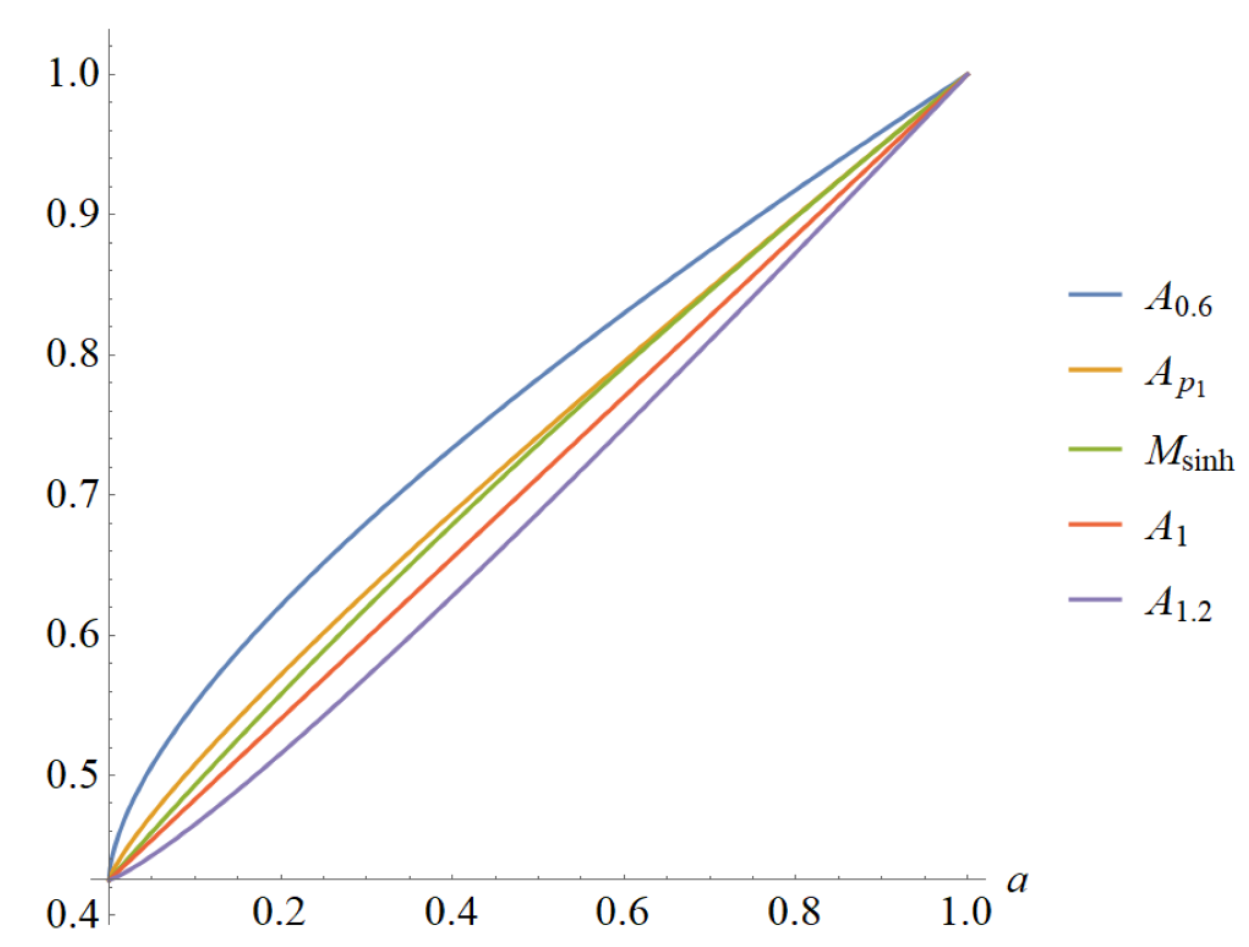
Figure 1. The graph of A p a , b ; α p and M sinh ( a , b ) when b = 1 and a ( 0 , 1 ) . From this, it can be observed that the double inequality (16) holds. The symmetric mean M sinh ( a , 1 ) is controlled by the asymmetric means A p ( a , 1 ; α p ) , with A 1 and A p 1 being its sharp lower and upper bounds.
Axioms 12 00910 g001
Figure 2. The graph of A p a , b ; α p M s i n h ( a , b ) when b = 1 and a ( 0 , 1 ) . A 1 ( a , 1 ; α 1 ) and A p 1 ( a , 1 ; α p 1 ) represent the sharp lower and upper bounds of M sinh . Once exceeded, they are inevitably breached, as illustrated by the example A 0.9 ( a , 1 ; α 0.9 ) taken here.
Axioms 12 00910 g002
Figure 3. The graph of A p a , b ; β p and M tan ( a , b ) when b = 1 and a ( 0 , 1 ) . From this, it can be observed that the double inequality (18) holds. The symmetric mean M tan ( a , 1 ) is controlled by the asymmetric means A p ( a , 1 ; β p ) , with A 1 and A p 0 being its sharp lower and upper bounds.
Axioms 12 00910 g003
Figure 4. The graph of A p a , b ; β p M t a n ( a , b ) when b = 1 and a ( 0 , 1 ) . A 1 ( a , 1 ; β 1 ) and A p 0 ( a , 1 ; β p 0 ) represent the sharp lower and upper bounds of M tan . Once exceeded, they are inevitably breached, as illustrated by the example A 0.7 ( a , 1 ; β 0.7 ) taken here.
Axioms 12 00910 g004
Figure 5. U sinh / V for different values of the parameter p.
Axioms 12 00910 g005
Figure 6. U tan / V for different values of the parameter p.
Axioms 12 00910 g006
Disclaimer/Publisher’s Note: The statements, opinions and data contained in all publications are solely those of the individual author(s) and contributor(s) and not of MDPI and/or the editor(s). MDPI and/or the editor(s) disclaim responsibility for any injury to people or property resulting from any ideas, methods, instructions or products referred to in the content.