Bayesian Estimation Using Product of Spacing for Modified Kies Exponential Progressively Censored Data

Abstract

In life testing and reliability studies, most researchers have used the maximum likelihood estimation method to estimate unknown parameters, even though it has been proven that the maximum product of spacing method has properties as good as the maximum likelihood estimation method and sometimes even better. In this study, we aim to estimate the unknown parameters of the modified Kies exponential distribution along with the reliability and hazard rate functions under progressive type-II censoring scheme. The maximum likelihood and maximum product of spacing methods are considered in order to find the point estimates and approximate confidence intervals of the various parameters. Moreover, Bayesian estimations based on the likelihood function and the product of the spacing function of the unknown parameters are obtained using the squared error loss function with independent gamma priors. It is observed that the joint posterior distributions have complicated forms. Because of this, Lindley’s approximation and the Markov chain Monte Carlo technique are used to obtain the Bayesian estimates and highest posterior credible intervals. Monte Carlo simulations are performed in order to evaluate the performance of the proposed estimation methods. Two real datasets are studied to demonstrate the efficacy of the offered methodologies and highlight how simple and applicable it might be to apply them in practical fields.

1. Introduction

Lifetime distributions are useful statistical tools for modeling many properties of lifetime data. Recently, many lifetime distributions have been proposed to add more flexibility in analysing lifetime data. One of the most important proposed distributions is the modified Kies exponential (MKiEx), proposed by Al-Babtain et al. [1]. Let X be a random variable that follows the MKiEX distribution; then, according to Al-Babtain et al. [1], the cumulative distribution function (CDF) of X is

$$\begin{array}{c}\hfill F(x;a,\lambda )=1-e^{-{(e^{\lambda x}-1)}^a}.\end{array}$$

(1)

The corresponding probability density function (PDF) is provided by

$$\begin{array}{c}\hfill f(x;a,\lambda )=a\lambda e^{\lambda ax}{(1-e^{-\lambda x})}^{a-1}{e}^{-{(e^{\lambda x}-1)}^a}.\end{array}$$

(2)

The reliability function (RF) and hazard rate function (HRF) at mission time $t>0$ are respectively provided by

$$\begin{array}{c}\hfill R\left(t\right)=1-F(t;a,\lambda )=e^{-{(e^{\lambda t}-1)}^a}\end{array}$$

(3)

and

$$\begin{array}{c}\hfill h\left(t\right)=a\lambda e^{\lambda at}{(1-e^{-\lambda t})}^{a-1}.\end{array}$$

(4)

The MKiEx distribution has two parameters, the shape parameter a and the scale parameter $\lambda$. Al-Babtain et al. [1] showed that the density function of the MKiEx distribution can take different shapes based on the shape parameter a. The hazard rate function of the MKiEx distribution can be increasing and bathtub-shaped. Using real datasets, Al-Babtain et al. [1] proved that the MKiEx distribution performs better than a number of other distributions, such as exponential distributions and gamma distributions. Several studies have considered the estimation of the MKiEx distribution; for example, see Aljohani et al. [2], Nassar and Alam [3] and El-Raheem et al. [4].

In practice, testing the whole sample takes time. Therefore, it is recommended to stop the test before the whole sample size fails in order to save time and cost. In this case, the test produces censored data. In this procedure, the lifetimes of the first $m(m<n)$ failed items are observed and the rest of the $(n-m)$ items are unobserved, i.e., censored. The main two types of conventional censoring schemes are type-I and type-II censoring. In the type-I censoring scheme, the n items are placed under the test and the test is stopped at a prespecified time T. The sample obtained from the test is called a time-censored sample, and the number of observed data in this case is random. On the other hand, in type-II censoring schemes the n items are placed under test and the test is stopped at a preset number of failures $m<n$; in this case, the sample obtained from the test is called a failure-censored sample. Here, the termination time of the test is random. The conventional type-I and type-II censoring schemes are not flexible enough in removing items which only happen when the experiment is terminated. Because of this, progressive censoring schemes which contain a more general censoring plan have been introduced. In progressive type-II censoring, $R_1$ items are discarded from the $n-1$ remaining items when the first failure occurs. Likewise, $R_2-2$ units are randomly removed from the $n-2-R_1$ remaining items at the time of the second failure. This procedure continues until the $m-th$ unit fails. It is important to mention here that m and ($R_1,\dots ,R_m$) are predetermined in advance. In the case of progressive type-II censoring, the likelihood function (LF) can be expressed as

$$\begin{array}{c}\hfill L\left(\mathit{\theta }\right)=C\prod _{i=1}^{m}f(x_{\left(i\right)};\mathit{\theta }){[1-F\left(x_{\left(i\right)}\right)]}^{R_i},\end{array}$$

(5)

where C is a constant and $\mathit{\theta }$ is the vector of the unknown parameters. Note that $x_{\left(1\right)},\dots ,x_{\left(m\right)}$ are the realizations of $X_{\left(1\right)},\dots ,X_{\left(m\right)}$. Many studies have investigated the estimation of the unknown parameters of various lifetime distributions under progressive type-II censoring schemes, including Ng et al. [5], Singh et al. [6], Alshenawy et al. [7], and Lin et al. [8]. For more details about censoring schemes, see Balakrishnan and Cramer [9] and Lawless [10].

In certain distributions, especially three or more parameter distributions, the ML estimation method can break down. Due to this, estimators may become inconsistent. The maximum product of spacing (MPS) method was proposed by Cheng and Amin [11] as a new alternative to the ML method. The spacings are the differences between the values of the CDF of two consecutive datapoints that are uniformly distributed on the interval $[0,1]$. The MPS method chooses the parameter value that makes the spacings as uniform as possible by maximizing the geometric mean of the spacings. According to Cheng and Amin [11], the MPS and ML estimation approaches are asymptotically identical and share the same characteristics of asymptotic sufficiency, consistency, and efficiency. Ranneby [12] proved that the MPS estimator has the same invariance property as the ML method. He showed that in certain situations the MPS method performs better than the ML estimation method, especially in cases with small sample sizes. According to Ng et al. [5], the product of the spacing function (PSF) under progressive type-II censoring becomes

$$\begin{array}{c}\hfill S\left(\mathit{\theta }\right)=C\prod _{i=1}^{m+1}{\delta }_i\left(\mathit{\theta }\right)\prod _{i=1}^m{[1-F\left(x_{\left(i\right)}\right)]}^{R_i},\end{array}$$

(6)

where C is a constant and

$$\begin{array}{c}\hfill {\delta }_i\left(\mathit{\theta }\right)=F(x_{\left(i\right)};\mathit{\theta })-F(x_{(i-1)};\mathit{\theta }),i=1,2,\dots ,m+1,\end{array}$$

where $F(x_{\left(0\right)};\mathit{\theta })=0$ and $F(x_{(m+1)};\mathit{\theta })=1$. Many authors have used the MPS method to obtain estimates of the unknown parameters of lifetime models. Rahman and Pearson [13] used ML estimation and the MPS methods to obtain the estimates of the two-parameter exponential distribution. Singh et al. [14] obtained the point and asymptotic interval estimations of the parameters of generalized inverted exponential distributions using the MPS, ML, and least squares methods. For more, see the works of Singh et al. [6], Rahman et al. [15], Aruna [16], Teimouri and Nadarajah [17], Almetwally et al. [18], and Tashkandy et al. [19].

We are motivated to conduct the present work because of (1) the flexibility of the MKiEx distribution and its ability to model different types of data; (2) the efficiency of the progressive type-II censoring scheme in terminating the experiment as compared to conventional censoring schemes; (3) a lack of studies reported on estimation of the MKiEx distribution’s parameters using the MPS method and Bayesian estimation under PSF and the progressive type-II censoring scheme; and (4) the need to conduct a comparative study; here, we compare six estimation methods to determine the best performing method. Furthermore, Lindley’s approximation for the Bayesian estimation under PSF has not yet been studied. Thus, our main objective in this study is to discuss the estimation of the unknown parameters of the MKiEx distribution under progressive Type-II data. The RF and HRF are estimated as well. To achieve this, the ML, MPS, and Bayesian estimations are considered under the LF and PSF methods. Based on the asymptotic properties of the ML estimates (MLEs) and the MPS estimates (MPSEs), the approximate confidence intervals (ACIs) of the unknown parameters RF and HRF are obtained. The Bayesian estimates are calculated through the Monte Carlo Markov Chain (MCMC) procedure and Lindley’s approximation using the squared error loss function (SELF). The highest posterior density (HPD) credible intervals of the unknown parameters are investigated, along with the RF and HRF. A simulation study and two applications are provided to compare the various techniques and show the applicability of the proposed methods.

This article’s remaining sections are organized as follows. In Section 2, the ML method is applied to find the point and interval estimates of the unknown parameters. Section 3 discusses the point and interval estimations of the parameters using the MPS method. In Section 4, we conduct Bayesian estimation based on LF. Bayesian estimation based on PSF is considered in Section 5. The performance of the suggested methods is investigated through a simulation study in Section 6. The analysis of two real datasets is presented in Section 7. Finally, our conclusions are provided in Section 8.

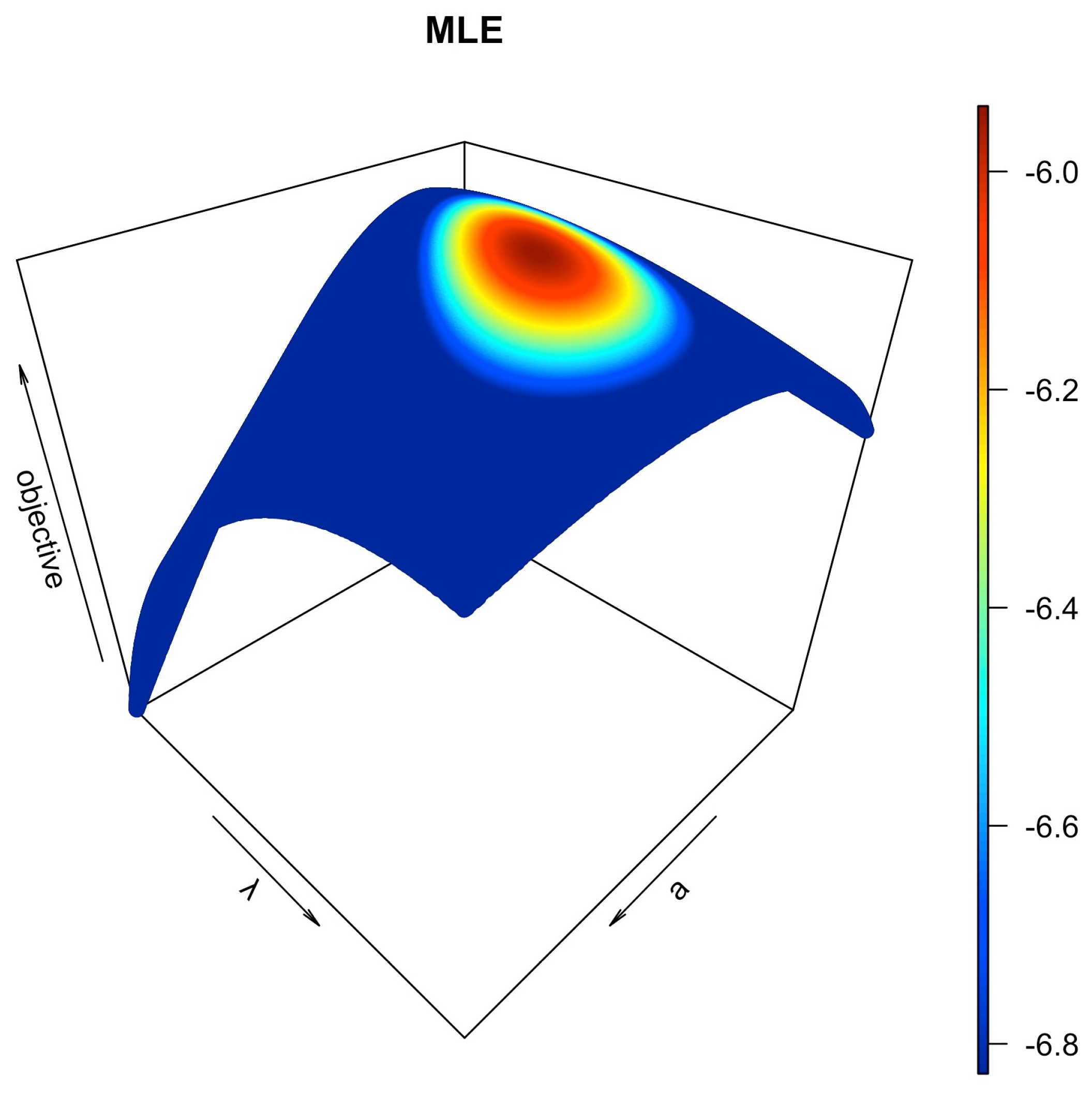
2. Maximum Likelihood Estimation

Let $x_{\left(1\right)},x_{\left(2\right)},\dots ,x_{\left(m\right)}$ be a progressively type-II censored sample taken from a population that follows the MKiEx distribution, with the CDF and PDF provided by (1) and (2), respectively, and with a progressive censoring plan $(R_1,R_2,\dots ,R_m)$. For simplicity, let $x_i=x_{\left(i\right)}$ and $A_i=e^{\lambda x_i}-1$. From (1), (2), and (5), the LF and its logarithm without the constant term become

$$\begin{array}{c}\hfill L(a,\lambda )={\left(a\lambda \right)}^{m}exp\left[\lambda a\sum _{i=1}^m{x}_i-\sum _{i=1}^m(R_i+1)A_i^a\right]\prod _{i=1}^m{(1-e^{-\lambda x_i})}^{a-1}\end{array}$$

(7)

and

$$\begin{array}{c}\hfill l(a,\lambda )=mlog\left(a\lambda \right)+\lambda a\sum _{i=1}^m{x}_i-\sum _{i=1}^m(R_i+1)A_i^a+(a-1)\sum _{i=1}^{m}log(1-e^{-\lambda x_i}).\end{array}$$

(8)

The MLEs of the two parameters a and $\lambda$ of the MKiEx distribution, denoted by $\widehat{a}$ and $\widehat{\lambda }$, are acquired by solving the following two nonlinear equations simultaneously:

$$\begin{array}{c}\hfill \frac{\partial l(a,\lambda )}{\partial a}=\frac{m}{a}+\lambda \sum _{i=1}^m{x}_i+\sum _{i=1}^{m}log(1-e^{-\lambda x_i})-\sum _{i=1}^m(R_i+1)A_i^{a}log\left(A_i\right)=0\end{array}$$

(9)

and

$$\begin{array}{c}\hfill \frac{\partial l(a,\lambda )}{\partial \lambda }=\frac{m}{\lambda }+a\sum _{i=1}^m{x}_i+(a-1)\sum _{i=1}^m{x}_i{A}_i^{-1}-a\sum _{i=1}^m(R_i+1)x_i{e}^{\lambda x_i}{A}_i^{a-1}=0.\end{array}$$

(10)

It is hard to solve the previous equations in explicit form. Therefore, we use the Newton–Raphson method to solve these equations numerically. The MLEs of RF and HRF can be found using the invariance property of the MLEs by replacing a and $\lambda$ in (3) and (4) by $\widehat{a}$ and $\widehat{\lambda }$, respectively. Thus,

$$\begin{array}{c}\hfill \widehat{R}\left(t\right)=e^{-{(e^{\widehat{\lambda }t}-1)}^{\widehat{a}}}\mathrm{and}\widehat{H}\left(t\right)=\widehat{a}\widehat{\lambda }{e}^{\widehat{\lambda }at}{(1-e^{-\widehat{\lambda }t})}^{\widehat{a}-1}.\end{array}$$

We must confirm the existence and uniqueness of a and $\lambda$ before obtaining their estimates. Due to the complex form of the normal equations, we can use graphical techniques to check them. A three-dimensional (3D) plot is created for the log-LF in (8) using a simulated sample from the MKiEx distribution under the progressive censoring plan $R_1=R_2=\dots =R_9=0$ and $R_{10}=20$, with $a=1$ and $\lambda =1$, as shown in Figure 1. The 3D plot clearly shows that there are areas where there exist global extrema, which might indicate that the MLEs exist and are unique. The Fisher information is a method of calculating the amount of information carried by an observed random sample about unknown parameters a and $\lambda$. The Fisher information matrix can be defined as

$$\begin{array}{c}\hfill I(a,\lambda )=E\left(\begin{array}{cc}-\frac{{\partial }^{2}l(a,\lambda )}{\partial a^2}& -\frac{{\partial }^{2}l(a,\lambda )}{\partial a\partial \lambda }\\ -\frac{{\partial }^{2}l(a,\lambda )}{\partial \lambda \partial a}& -\frac{{\partial }^{2}l(a,\lambda )}{\partial {\lambda }^2}\end{array}\right);\end{array}$$

for more details, see DeGroot and Schervish [20]. In many cases, it is not possible to obtain explicit mathematical expressions for the previous expectation; therefore, Cohen [21] considered using the observed Fisher information by substituting $(a,\lambda )$ with $(\widehat{a},\widehat{\lambda })$. In this case, the asymptotic variance–covariance matrix of the MLEs can be written as follows:

$$\begin{array}{ccc}\hfill I^{-1}(\widehat{a},\widehat{\lambda })& =& {\left.{\left(\begin{array}{cc}-\frac{{\partial }^{2}l(a,\lambda )}{\partial a^2}& -\frac{{\partial }^{2}l(a,\lambda )}{\partial a\partial \lambda }\\ -\frac{{\partial }^{2}l(a,\lambda )}{\partial \lambda \partial a}& -\frac{{\partial }^{2}l(a,\lambda )}{\partial {\lambda }^2}\end{array}\right)}^{-1}\right|}_{(a,\lambda )=(\widehat{a},\widehat{\lambda })}\hfill \\ & =& \left(\begin{array}{cc}\widehat{var}\left(\widehat{a}\right)& \widehat{cov}(\widehat{a},\widehat{\lambda })\\ \widehat{cov}(\widehat{\lambda },\widehat{a})& \widehat{var}\left(\widehat{\lambda }\right)\end{array}\right),\hfill \end{array}$$

(11)

where $\frac{{\partial }^{2}l(a,\lambda )}{\partial a^2}$,$\frac{{\partial }^{2}l(a,\lambda )}{\partial {\lambda }^2}$ and $\frac{{\partial }^{2}l(a,\lambda )}{\partial a\partial \lambda }$ are shown in Appendix A.

Under mild regularity conditions, it is known that the MLEs are asymptotically normally distributed, i.e., $(\widehat{a},\widehat{\lambda })\sim N[(a,\lambda ),I^{-1}(\widehat{a},\widehat{\lambda })]$; for more details, see Casella and Berger [22]. Therefore, we can calculate the ACI based on the asymptotic properties of the MLEs. Hence, the $100(1-\gamma )\%$ ACIs of a and $\lambda$ based on the MLEs are

$$\begin{array}{c}\hfill \widehat{a}\pm z_{\gamma /2}\sqrt{\widehat{var}\left(\widehat{a}\right)}\mathrm{and}\widehat{\lambda }\pm z_{\gamma /2}\sqrt{\widehat{var}\left(\widehat{\lambda }\right)},\end{array}$$

respectively, where $z_{\gamma }$ is the γth percentile of a standard normal distribution.

To find the ACIs for the RF and HRF, the delta method (see, e.g., Greene [23]) can be used to obtain the approximate estimates of the variances associated with the MLEs of RF and HRF. According to the delta method, the approximate estimates of the variances of RF and HRF based on (11) are

$$\begin{array}{c}\hfill \widehat{var}\left(\widehat{R}\right)={\left[{\acute{G}}_1{I}^{-1}(\widehat{a},\widehat{\lambda })G_1\right]}_{(a,\lambda )=(\widehat{a},\widehat{\lambda })}\mathrm{and}\widehat{var}\left(\widehat{h}\right)={\left[{\acute{G}}_2{I}^{-1}(\widehat{a},\widehat{\lambda })G_2\right]}_{(a,\lambda )=(\widehat{a},\widehat{\lambda })},\end{array}$$

respectively, where

$$\begin{array}{c}\hfill {\acute{G}}_1=\left(\frac{\partial R\left(t\right)}{\partial a},\frac{\partial R\left(t\right)}{\partial \lambda }\right)\mathrm{and}{\acute{G}}_2=\left(\frac{\partial h\left(t\right)}{\partial a},\frac{\partial h\left(t\right)}{\partial \lambda }\right).\end{array}$$

The elements of ${\acute{G}}_1$ and ${\acute{G}}_2$ are provided by

$$\begin{array}{c}\hfill \frac{\partial R\left(t\right)}{\partial a}=-e^{-{(e^{\lambda t}-1)}^a}{(e^{\lambda t}-1)}^{a}log(e^{\lambda t}-1),\end{array}$$

$$\begin{array}{c}\hfill \frac{\partial R\left(t\right)}{\partial \lambda }=-at{e}^{e^{\lambda t}-{(e^{\lambda t}-1)}^a}{(e^{\lambda t}-1)}^{a-1},\end{array}$$

$$\begin{array}{c}\hfill \frac{\partial h\left(t\right)}{\partial a}=\lambda e^{(a+1)\lambda t}{(1-e^{-\lambda t})}^a(a\lambda t+alog(1-e^{-\lambda t})+1){(e^{\lambda t}-1)}^{-1}\end{array}$$

and

$$\begin{array}{c}\hfill \frac{\partial h\left(t\right)}{\partial \lambda }=a{e}^{(a+1)\lambda t}{(1-e^{-\lambda t})}^a\{e^{\lambda t}[a\lambda t+1]-\lambda t-1\}{(e^{\lambda t}-1)}^{-2}.\end{array}$$

In this case, the $100(1-\gamma )\%$ ACIs of RF and HRF based on the MLEs are respectively provided by

$$\begin{array}{c}\hfill \widehat{R}\left(t\right)\pm z_{\gamma /2}\sqrt{\widehat{var}\left(\widehat{R}\left(t\right)\right)}\mathrm{and}\widehat{h}\left(t\right)\pm z_{\gamma /2}\sqrt{\widehat{var}\left(\widehat{h}\left(t\right)\right)}.\end{array}$$

3. Maximum Product of Spacing Estimation

Let $x_{\left(1\right)},x_{\left(2\right)},\dots ,x_{\left(m\right)}$ be a progressively type-II censored sample taken from an MKiEx population with a CDF and PDF provided by (1) and (2), respectively, and with a progressive censoring strategy $(R_1,R_2,\dots ,R_m)$. Then, based on (1), (2), and (6) and ignoring the constant term, the PSF and the associated logarithm function are provided by

$$\begin{array}{c}\hfill S\left(a,\lambda \right)=e^{-{\sum }_{i=1}^m{R}_i{A}_i^a}\prod _{i=1}^{m+1}{\delta }_i\end{array}$$

(12)

and

$$\begin{array}{c}\hfill s\left(a,\lambda \right)=\sum _{i=1}^{m+1}log\left({\delta }_i\right)-\sum _{i=1}^m{R}_i{A}_i^a,\end{array}$$

(13)

respectively, where ${\delta }_i=e^{-{A_{i-1}}^a}-e^{-A_i^a}$. The MPSEs of the unknown parameters, denoted by $\tilde{a}$ and $\tilde{\lambda }$, are obtained by simultaneously solving the following normal equations:

$$\begin{array}{c}\hfill \frac{\partial s\left(a,\lambda \right)}{\partial a}=\sum _{i=1}^{m+1}\frac{{\varphi }_{1i}-{\varphi }_{1i-1}}{{\delta }_i}-\sum _{i=1}^m{R}_i{A}_i^{a}log\left(A_i\right)=0\end{array}$$

(14)

and

$$\begin{array}{c}\hfill \frac{\partial s\left(a,\lambda \right)}{\partial \lambda }=\sum _{i=1}^{m+1}\frac{{\varphi }_{2i}-{\varphi }_{2i-1}}{{\delta }_i}-a\sum _{i=1}^m{R}_i{x}_i{e}^{\lambda x_i}{A_i}^{a-1}=0,\end{array}$$

(15)

where ${\varphi }_{1i}=e^{-A_i^a}{A}_i^{a}log\left(A_i\right)$ and ${\varphi }_{2i}=a{x}_i{e}^{\lambda x_i-A_i^a}{A_i}^{a-1}$. The previous equations are difficult to explicitly solve. In order to numerically solve these equations, we use the Newton–Raphson method, as in the case of the MLEs. The MPSEs of the RF and HRF can be acquired by employing the invariance property, replacing a and $\lambda$ in (3) and (4) by $\tilde{a}$ and $\tilde{\lambda }$. Then, we can obtain the MPSEs of $R\left(t\right)$ and $h\left(t\right)$, respectively, as follows:

$$\begin{array}{c}\hfill \tilde{R}\left(t\right)=e^{-{(e^{\tilde{\lambda }t}-1)}^{\tilde{a}}}\mathrm{and}\tilde{h}\left(t\right)=\tilde{a}\tilde{\lambda }{e}^{\tilde{\lambda }at}{(1-e^{-\tilde{\lambda }t})}^{\tilde{a}-1}.\end{array}$$

Using the same simulated sample as in the previous section, Figure 2 presents the 3D plot for the Log-PSF in (13), which we can use to check the existence and uniqueness of the MPSEs $\tilde{a}$ and $\tilde{\lambda }$. From Figure 2, it can be concluded that the MPSEs might exist and may be unique.

Utilizing the asymptotic properties of the MPSEs, we can find the ACIs for $a,\lambda ,R\left(t\right)$, and $h\left(t\right)$. In this case, the asymptotic variance–covariance matrix of the MPSEs can be expressed as follows:

$$\begin{array}{ccc}\hfill I^{-1}(\tilde{a},\tilde{\lambda })& =& {\left.{\left(\begin{array}{cc}-\frac{{\partial }^{2}l(a,\lambda )}{\partial a^2}& -\frac{{\partial }^{2}l(a,\lambda )}{\partial a\partial \lambda }\\ -\frac{{\partial }^{2}l(a,\lambda )}{\partial \lambda \partial a}& -\frac{{\partial }^{2}l(a,\lambda )}{\partial {\lambda }^2}\end{array}\right)}^{-1}\right|}_{(a,\lambda )=(\tilde{a},\tilde{\lambda })}\hfill \\ & =& \left(\begin{array}{cc}\widetilde{var}\left(\tilde{a}\right)& \widetilde{cov}(\tilde{a},\tilde{\lambda })\\ \widetilde{cov}(\tilde{\lambda },\tilde{a})& \widetilde{var}\left(\tilde{\lambda }\right)\end{array}\right),\hfill \end{array}$$

(16)

where $\frac{{\partial }^{2}s(a,\lambda )}{\partial a^2}$, $\frac{{\partial }^{2}s(a,\lambda )}{\partial {\lambda }^2}$, and $\frac{{\partial }^{2}s(a,\lambda )}{\partial a\partial \lambda }$ are shown in Appendix B. Hence, the $100(1-\gamma )\%$ ACIs of a and $\lambda$ based on the MPSEs are

$$\begin{array}{c}\hfill \tilde{a}\pm z_{\gamma /2}\sqrt{\widetilde{var}\left(\tilde{a}\right)}\mathrm{and}\tilde{\lambda }\pm z_{\gamma /2}\sqrt{\widetilde{var}\left(\tilde{\lambda }\right)},\end{array}$$

respectively. To find the ACIs for the RF and HRF, we first approximate the estimates of the variances of RF and HRF based on (16). Thus,

$$\begin{array}{c}\hfill \widetilde{var}\left(\tilde{R}\right)={\left[{\acute{G}}_1{I}^{-1}(\tilde{a},\tilde{\lambda })G_1\right]}_{(a,\lambda )=(\tilde{a},\tilde{\lambda })}\mathrm{and}\widetilde{var}\left(\tilde{h}\right)={\left[{\acute{G}}_2{I}^{-1}(\tilde{a},\tilde{\lambda })G_2\right]}_{(a,\lambda )=(\tilde{a},\tilde{\lambda })},\end{array}$$

respectively. As a result, the respective $100(1-\gamma )\%$ ACIs of RF and HRF based on the MPSEs are provided by

$$\begin{array}{c}\hfill \tilde{R}\left(t\right)\pm z_{\gamma /2}\sqrt{\widetilde{var}\left(\tilde{R}\left(t\right)\right)}\mathrm{and}\tilde{h}\left(t\right)\pm z_{\gamma /2}\sqrt{\widetilde{var}\left(\tilde{h}\left(t\right)\right)}.\end{array}$$

4. LF-Based Bayesian Estimation

In this section, the Bayesian estimations of a, $\lambda$, RF, and HRF are considered when the derivation of the joint posterior distribution is LF-based. The Bayesian estimation method assumes that the unknown parameters are random variables with prior information. In the case of the MKiEX model, we consider that the prior distributions of a and $\lambda$ are independent, where the prior distribution of a is Gamma($a_1$, $b_1$) and the prior distribution of $\lambda$ is Gamma($a_2$, $b_2$). As a result, the joint prior distribution of a and $\lambda$ is

$$\begin{array}{c}\hfill p(a,\lambda )\propto a^{a_1-1}{\lambda }^{a_2-1}{e}^{-(b_{1}a+b_2\lambda )},a_j,b_j>0,j=1,2,\end{array}$$

(17)

where we choose to use the gamma prior due to its mathematical flexibility and ability to cover a wide range of prior beliefs held by the experimenter; for more details, see Fathi et al. [24], Eliwa et al. [25], and Dey et al. [26]. By combining the LF in (7) and the joint prior distribution (17), the joint posterior distribution is provided by

$$\begin{array}{ccc}\hfill g(a,\lambda |\mathbf{x})& =& B_1^{-1}{a}^{m+a_1-1}{\lambda }^{{m+a}_2-1}exp\left[\lambda \left(a\sum _{i=1}^m{x}_i-b_2\right)-\sum _{i=1}^m\left(R_i+1\right)A_i^a-b_{1}a\right]\hfill \\ & \times & \prod _{i=1}^m{(1-e^{-\lambda x_i})}^{a-1},\hfill \end{array}$$

(18)

where $\mathbf{x}$ is the data vector and

$$\begin{array}{ccc}\hfill B_1& =& {\int }_0^{\infty }{\int }_0^{\infty }{a}^{m+a_1-1}{\lambda }^{{m+a}_2-1}exp\left[\lambda \left(a\sum _{i=1}^m{x}_i-b_2\right)-\sum _{i=1}^m\left(R_i+1\right)A_i^a-b_{1}a\right]\hfill \\ & & \prod _{i=1}^m{(1-e^{-\lambda x_i})}^{a-1}dad\lambda .\hfill \end{array}$$

Using SELF, the Bayes estimator of any function of the parameters, say, $U(a,\lambda )$, can be obtained as follows:

$$\begin{array}{c}\hfill {\widehat{U}}_B(a,\lambda )={\int }_0^{\infty }{\int }_0^{\infty }U(a,\lambda )g(a,\lambda |\mathbf{x})dad\lambda \end{array}$$

(19)

It is complicated to obtain the Bayes estimator in (19) in explicit form; therefore, we propose using Lindley’s approximation and the MCMC technique to solve this difficulty in the preceding subsections.

4.1. Lindley’s Approximation

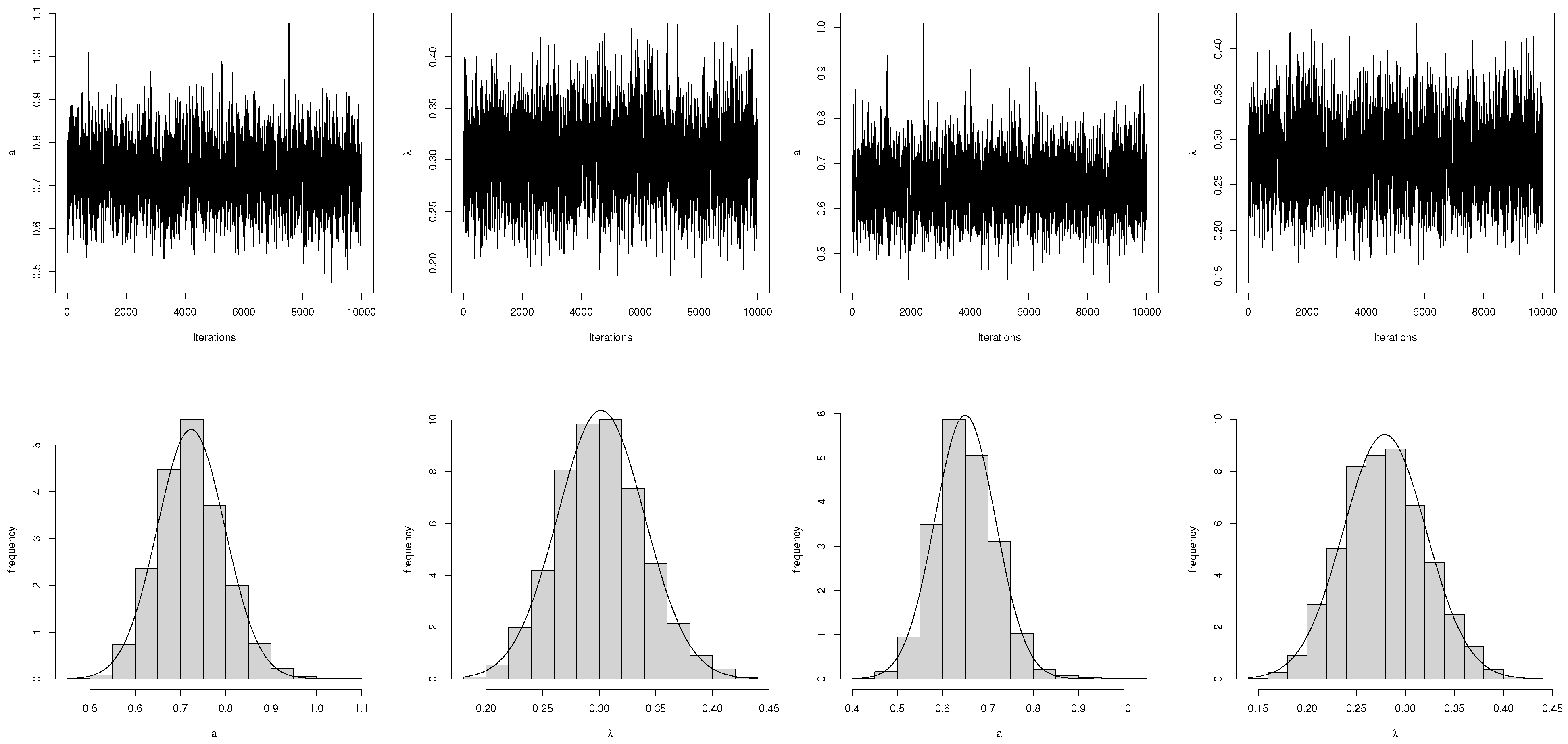
Lindley’s approximation was developed by Lindley [27] to obtain the Bayes estimators. Let $U(a,\lambda )$ be a function of the parameters a and $\lambda$ used to obtain the posterior expectation of $U(a,\lambda )$ as

$$\begin{array}{c}\hfill E\left[U(a,\lambda )\right]=\frac{\int U(a,\lambda )e^{l(a,\lambda )+\rho (a,\lambda )}d(a,\lambda )}{\int e^{l(a,\lambda )+\rho (a,\lambda )}d(a,\lambda )},\end{array}$$

(20)

where $l(a,\lambda )$ is log-LF and $\rho (a,\lambda )$ is the log of the joint priors of a and $\lambda$. The Bayes estimator of $U(a,\lambda )$ can be obtained using Lindley’s approximation by approaching the ratio of the integrals as a whole, producing a single numerical result using Taylor series expansion. The Lindley’s approximation form of the expression provided by (20) is

$$\begin{array}{ccc}\hfill E\left[U\right(a,\lambda \left)\right]& \approx & U(a,\lambda )+0.5[(u_{aa}+2u_a{\rho }_a){\sigma }_{aa}+(u_{\lambda a}+2u_{\lambda }{\rho }_a){\sigma }_{\lambda a}+(u_{a\lambda }+2u_a{\rho }_{\lambda }){\sigma }_{a\lambda }\hfill \\ & +& (u_{\lambda \lambda }+2u_{\lambda }{\rho }_{\lambda }){\sigma }_{\lambda \lambda }]+0.5[(u_a{\sigma }_{aa}+u_{\lambda }{\sigma }_{a\lambda })(q_{aaa}{\sigma }_{aa}+q_{a\lambda a}{\sigma }_{a\lambda }+q_{\lambda aa}{\sigma }_{\lambda a}\hfill \\ & +& q_{\lambda \lambda a}{\sigma }_{\lambda \lambda })+(u_a{\sigma }_{\lambda a}+u_{\lambda }{\sigma }_{\lambda \lambda })(q_{\lambda aa}{\sigma }_{aa}+q_{a\lambda \lambda }{\sigma }_{a\lambda }+q_{\lambda a\lambda }{\sigma }_{\lambda a}+q_{\lambda \lambda \lambda }{\sigma }_{\lambda \lambda })],\hfill \end{array}$$

(21)

where $u_a$, $u_{\lambda }$, $u_{a\lambda }$, $u_{\lambda a}$, $u_{aa}$, and $u_{\lambda \lambda }$ are the derivatives of $U(a,\lambda )$. All terms in (21) are evaluated at the MLEs $\widehat{a}$ and $\widehat{\lambda }$ of a and $\lambda$, respectively. The quantities in (21) are shown in Appendix C. In addition, from the joint prior distribution in (17) we have

$$\begin{array}{c}\hfill \rho (a,\lambda )=log\left[g(a,\lambda )\right]=(a_1-1)log\left(a\right)+(a_2-1)log\left(\lambda \right)-(b_{1}a+b_2\lambda ).\end{array}$$

Thus,

$$\begin{array}{c}\hfill {\rho }_a=\frac{a_1-1}{a}-b_1\end{array}$$

(22)

and

$$\begin{array}{c}\hfill {\rho }_{\lambda }=\frac{a_2-1}{\lambda }-b_2.\end{array}$$

(23)

Now, when $U(a,\lambda )=a$, we have $u_a=1$ and $u_{\lambda }=u_{aa}=u_{\lambda \lambda }=u_{a\lambda }=u_{\lambda a}=0$. Then, we can obtain the Bayesian estimator of a as follows:

$$\begin{array}{cc}\hfill {\widehat{a}}_{BL}& =\widehat{a}+{\Delta }_1,\hfill \end{array}$$

where

$$\begin{array}{ccc}\hfill {\Delta }_1& =& {\rho }_a{\sigma }_{aa}+{\rho }_{\lambda }{\sigma }_{a\lambda }+0.5[q_{aaa}{\sigma }_{aa}^2+3q_{aa\lambda }{\sigma }_{aa}{\sigma }_{a\lambda }+q_{a\lambda \lambda }{\sigma }_{aa}{\sigma }_{\lambda \lambda }\hfill \\ & +& 2q_{a\lambda \lambda }{\sigma }_{a\lambda }^2+q_{\lambda \lambda \lambda }{\sigma }_{a\lambda }{\sigma }_{\lambda \lambda }].\hfill \end{array}$$

(24)

Similarly, for $U(a,\lambda )=\lambda$ and $u_{\lambda }=1$,$u_a=u_{aa}=u_{\lambda \lambda }=u_{a\lambda }=u_{\lambda a}=0$, we can obtain the Bayesian estimator of $\lambda$ as follows:

$$\begin{array}{cc}\hfill {\widehat{\lambda }}_{BL}& =\widehat{\lambda }+{\Delta }_2,\hfill \end{array}$$

where

$$\begin{array}{ccc}\hfill {\Delta }_2& =& {\rho }_a{\sigma }_{\lambda a}+{\rho }_{\lambda }{\sigma }_{\lambda \lambda }+0.5[q_{aaa}{\sigma }_{aa}{\sigma }_{a\lambda }+2q_{aa\lambda }{\sigma }_{a\lambda }^2+3q_{a\lambda \lambda }{\sigma }_{a\lambda }{\sigma }_{\lambda \lambda }\hfill \\ & +& q_{aa\lambda }{\sigma }_{aa}{\sigma }_{\lambda \lambda }+q_{\lambda \lambda \lambda }{\sigma }_{\lambda \lambda }^2].\hfill \end{array}$$

(25)

We can obtain the Bayesian estimator of the RF using the same approach. For simplicity, let $A_t=e^{\lambda t}-1$ and $U(a,\lambda )=e^{-A_t^a}$; then, we have

$$\begin{array}{c}\hfill u_a=-e^{-A_t^a}{A}_t^{a}log\left(A_t\right),\end{array}$$

$$\begin{array}{c}\hfill u_{\lambda }=-at{e}^{\lambda t-A_t^a}{A}_t^{a-1},\end{array}$$

$$\begin{array}{c}\hfill u_{aa}=e^{-A_t^a}{A}_t^a(A_t^a-1){log}^2\left(A_t\right),\end{array}$$

$$\begin{array}{c}\hfill u_{\lambda \lambda }=a{t}^2{e}^{\lambda t-A_t^a}{A}_t^{a-2}(a{e}^{\lambda t}{A}_t^a-a{e}^{\lambda t}+1)\end{array}$$

$$\begin{array}{c}\hfill u_{a\lambda }=u_{\lambda a}=t{e}^{\lambda t-{(e^{\lambda t}-1)}^a}{A}_t^{a-1}[a(A_t^a-1)log\left(A_t\right)-1]\end{array}$$

Thus, the Bayesian estimator of the RF can be obtained as

$$\begin{array}{cc}\hfill {\widehat{R}}_{BL}& =\widehat{R}+{\Delta }_3,\hfill \end{array}$$

where

$$\begin{array}{ccc}\hfill {\Delta }_3& =& 0.5[(u_{aa}+2u_a{\rho }_a){\sigma }_{aa}+(u_{\lambda a}+2u_{\lambda }{\rho }_a){\sigma }_{\lambda a}+(u_{a\lambda }+2u_a{\rho }_{\lambda }){\sigma }_{a\lambda }+(u_{\lambda \lambda }+2u_{\lambda }{\rho }_{\lambda }){\sigma }_{\lambda \lambda }]\hfill \\ & +& 0.5[(u_a{\sigma }_{aa}+u_{\lambda }{\sigma }_{a\lambda })(q_{aaa}{\sigma }_{aa}+q_{a\lambda a}{\sigma }_{a\lambda }+q_{\lambda aa}{\sigma }_{\lambda a}+q_{\lambda \lambda a}{\sigma }_{\lambda \lambda })+(u_a{\sigma }_{\lambda a}+u_{\lambda }{\sigma }_{\lambda \lambda })\hfill \\ & \times & (q_{\lambda aa}{\sigma }_{aa}+q_{a\lambda \lambda }{\sigma }_{a\lambda }+q_{\lambda a\lambda }{\sigma }_{\lambda a}+q_{\lambda \lambda \lambda }{\sigma }_{\lambda \lambda })].\hfill \end{array}$$

(26)

For the HRF, let $B_t=1-e^{-\lambda t}$ and $U(a,\lambda )=a\lambda e^{\lambda at}{B}_t^{a-1}$; then, we have

$$\begin{array}{c}\hfill u_a=\lambda e^{a\lambda t}{B}_t^{a-1}[a(\lambda t+log\left(B_t\right))+1],\end{array}$$

$$\begin{array}{c}\hfill u_{\lambda }=a{e}^{\lambda t}{A}_t^{a-2}[e^{\lambda t}(a\lambda t+1)-\lambda t-1],\end{array}$$

$$\begin{array}{c}\hfill u_{aa}=\left[\lambda e^{(a+1)\lambda t}{B}_t^a(\lambda t+log\left(B_t\right))(a\lambda t+alog\left(B_t\right)+2)\right]A_t^{-1},\end{array}$$

$$\begin{array}{c}\hfill u_{\lambda \lambda }=at{e}^{\lambda t}{A}_t^{a-3}\{e^{\lambda t}[a(e^{\lambda t}\{a\lambda t+2\}-3\lambda t-2)+\lambda t-2]+\lambda t+2\},\end{array}$$

$$\begin{array}{c}\hfill u_{a\lambda }=u_{\lambda a}=e^{\lambda t}{A}_t^{a-2}\{e^{\lambda t}[2a\lambda t+1]+a[e^{\lambda t}(a\lambda t+1)-\lambda t-1]log\left(A_t\right)-\lambda t-1\}.\end{array}$$

Therefore, the Bayesian estimator of the HRF can be obtained as

$$\begin{array}{cc}\hfill {\widehat{h}}_{BL}& =\widehat{h}+{\Delta }_4,\hfill \end{array}$$

where

$$\begin{array}{ccc}\hfill {\Delta }_4& =& 0.5[(u_{aa}+2u_a{\rho }_a){\sigma }_{aa}+(u_{\lambda a}+2u_{\lambda }{\rho }_a){\sigma }_{\lambda a}+(u_{a\lambda }+2u_a{\rho }_{\lambda }){\sigma }_{a\lambda }+(u_{\lambda \lambda }+2u_{\lambda }{\rho }_{\lambda }){\sigma }_{\lambda \lambda }]\hfill \\ & +& 0.5[(u_a{\sigma }_{aa}+u_{\lambda }{\sigma }_{a\lambda })(q_{aaa}{\sigma }_{aa}+q_{a\lambda a}{\sigma }_{a\lambda }+q_{\lambda aa}{\sigma }_{\lambda a}+q_{\lambda \lambda a}{\sigma }_{\lambda \lambda })+(u_a{\sigma }_{\lambda a}+u_{\lambda }{\sigma }_{\lambda \lambda })\hfill \\ & \times & (q_{\lambda aa}{\sigma }_{aa}+q_{a\lambda \lambda }{\sigma }_{a\lambda }+q_{\lambda a\lambda }{\sigma }_{\lambda a}+q_{\lambda \lambda \lambda }{\sigma }_{\lambda \lambda })].\hfill \end{array}$$

(27)

4.2. MCMC Technique

In this subsection, we use the MCMC method to obtain the Bayesian estimates of a and $\lambda$ as well as $R\left(t\right)$ and $h\left(t\right)$. The MCMC technique can be used to simulate samples from (18), and in turn to obtain the Bayesian estimates. To generate samples from (18), we need to sample successively from a target distribution. Thus, in order to use the MCMC technique, we need to derive the full conditional distributions of a and $\lambda$, as follows:

$$\begin{array}{c}\hfill g\left(a\right|\lambda ,\mathbf{x})\propto a^{m+a_1-1}exp\{-a[-\lambda \sum _{i=1}^m{x}_i+b_1-log(1-e^{-\lambda x_i})]\}{e}^{-{\sum }_{i=1}^m(R_i+1){(e^{\lambda x_i}-1)}^a}\end{array}$$

(28)

and

$$\begin{array}{c}\hfill \begin{array}{cc}\hfill g\left(\lambda \right|a,\mathbf{x})& \propto {\lambda }^{{m+a}_2-1}exp\left[\sum _{i=1}^m(a-1)log(1-e^{-\lambda x_i})-(R_i+1){(e^{\lambda x_i}-1)}^a\right]\hfill \\ & e^{-\lambda (-a{\sum }_{i=1}^m{x}_i+b_2)}.\hfill \end{array}\end{array}$$

(29)

It can be seen that (28) and (29) cannot be reduced to any well-known distributions. Therefore, we have used the plots of these conditional distributions to show that the distributions in (28) and (29) behave similar to the normal distribution. Thus, we employ the Metropolis–Hastings (M-H) technique with normal proposal distributions, as follows:

Step 1

Set initial guess points for $(a^{\left(0\right)},{\lambda }^{\left(0\right)})$ as $(\widehat{a},\widehat{\lambda })$.

Step 2

Set $j=1$.

Step 3

Generate a* from $N(a^{(j-1)},\widehat{var}\left(\widehat{a}\right))$.

Step 4

Calculate $\beta =min[1,\frac{g_1\left(a^{*}\right|{\lambda }^{(j-1)},\mathbf{x})}{g_1\left(a^{(j-1)}\right|{\lambda }^{(j-1)},\mathbf{x})}]$.

Step 5

Generate a sample u from $U(0,1)$.

Step 6

If $u\le \beta$, accept the generated value and set $a^{\left(j\right)}=a^{*}$; otherwise, reject the proposed distribution and set $a^{\left(j\right)}=a^{(j-1)}$.

Step 7

Follow the same line as in steps in 3–6 to generate ${\lambda }^{\left(j\right)}$ from (29).

Step 8

Obtain $R^{\left(j\right)}\left(t\right)=e^{-{(e^{{\lambda }^{\left(j\right)}t}-1)}^{a^{\left(j\right)}}}$ and $h^{\left(j\right)}\left(t\right)=a^{\left(j\right)}{\lambda }^{\left(j\right)}{e}^{{\lambda }^{\left(j\right)}{a}^{\left(j\right)}t}{(1-e^{-{\lambda }^{\left(j\right)}t})}^{a^{\left(j\right)}-1}$.

Step 9

Set $j=j+1$.

Step 10

Repeat steps 3–9 M times and obtain M random samples of a,$\lambda$,$R\left(t\right)$ and $h\left(t\right)$ as $\{a^{\left(1\right)},a^{\left(2\right)},\dots ,a^{\left(M\right)}\}$, $\{{\lambda }^{\left(1\right)},{\lambda }^{\left(2\right)},\dots ,{\lambda }^{\left(M\right)}\}$, $\{R^{\left(1\right)}\left(t\right),R^{\left(2\right)}\left(t\right),\dots ,R^{\left(M\right)}\left(t\right)\}$

and $\{h^{\left(1\right)}\left(t\right),h^{\left(2\right)}\left(t\right),\dots ,h^{\left(M\right)}\left(t\right)\}$, respectively.

Step 11

The LF-based Bayes estimates using a, $\lambda$, $R\left(t\right)$, and $h\left(t\right)$ (say, $\theta$) under SELF are provided by

$$\begin{array}{c}\hfill {\widehat{\theta }}_{BM}=E\left(\theta \right|\mathbf{x})=\frac{1}{M-Q}\sum _{j=Q+1}^M{\theta }^{\left(j\right)},\end{array}$$

where Q is the burn-in period.

Step 12

Follow the approach suggested by Chen and Shao [28] to obtain the HPD credible interval of the parameter $\theta$, as follows:

• Arrange the MCMC chain of $\theta$ after the burn-in period to obtain $({\theta }^{(Q+1)},\dots ,{\theta }^{\left(M\right)})$.
• In this case, the two-sided $100(1-\gamma )\%$ HPD credible interval of $\theta$ can be found as follows:

  $$\begin{array}{c}\hfill \left\{{\theta }^{\left(j^{*}\right)},{\theta }^{(j^{*}+\left((1-\gamma )(M-Q)\right)}\right\},\end{array}$$

  (30)

  where $j^{*}=Q+1,Q+2,\dots ,M$ is selected such that

  $$\begin{array}{c}\hfill {\theta }^{(j^{*}+\left[(1-\gamma )(M-Q)\right])}-{\theta }^{\left(j^{*}\right)}=\underset{1\le j\le \gamma (M-Q)}{min}\left({\theta }^{(j+[(1-\gamma )(M-Q)\left]\right)}-{\theta }^{\left(j\right)}\right),\end{array}$$

  (31)

where [h] denotes the largest integer less than or equal to h.

5. PSF-Based Bayesian Estimation

The standard Bayesian approach uses the LF to obtain the information from the sample. Coolen and Newby [29] have stated that there are two problems that occur when using the LF in the Bayesian method: (i) the LF is unbounded in certain cases, and (ii) the LF is sensitive to outliers. The unboundedness of the LF can be a serious barrier in Bayesian analysis. According to Cohen and Whitten [30], the unbounded likelihood problem typically arises when the unknown parameter is within the range of the support of PDF. Cheng and Amin [11] proved that the MLE is bound to fail for any PDFs which are heavy-tailed or J-shaped. In these circumstances, finding a posterior density function for the unknown parameter may be difficult. Therefore, Coolen and Newby [29] suggested the use of the PSF in Bayesian analysis instead of the LF. They justified this because the PSF is an approximation of the LF, and the product of the spacing is actually a probability function. They concluded that there are no theoretical problems related to using the PSF in place of the LF in Bayesian estimation. Furthermore, they showed that the numerical behaviour of the product of the spacing is better than the likelihood. Basu et al. [31] proved that the Bayesian approach with the PSF can perform better than Bayesian estimation with the LF. Dey et al. [26] derived the estimates of the gamma distribution with progressive type-II censoring data using the Bayesian method based on the LF and PSF, then compares it to the ML and MPS methods. In addition, Nassar and Elshahhat [32] conducted a statistical analysis of inverse Weibull constant-stress partially accelerated life tests with adaptive progressively type-I censored data using the methods of ML, MPS, and Bayesian estimation based on the LF and PSF. In this section, the Bayesian estimation of the various parameters of the MKiEx distribution is considered. By combining the PSF in (12) and the joint prior distribution (17), the joint posterior distribution of the unknown parameters a and $\lambda$ can be expressed as follows:

$$\begin{array}{ccc}\hfill g(a,\lambda |\mathbf{x})& =& B_2^{-1}{a}^{a_1-1}{\lambda }^{a_2-1}{e}^{-(b_{1}a+b_2\lambda )-{\sum }_m^{i=1}{R}_i{A}_i^a}\prod _{i=1}^{m+1}\left[e^{-{A_{i-1}}^a}-e^{-A_i^a}\right]\hfill \end{array}$$

(32)

where

$$\begin{array}{ccc}\hfill B_2& =& {\int }_0^{\infty }{\int }_0^{\infty }a{a}^{a_1-1}{\lambda }^{a_2-1}{e}^{-(b_{1}a+b_2\lambda )-{\sum }_m^{i=1}{R}_i{A}_i^a}\prod _{i=1}^{m+1}\left[e^{-{A_{i-1}}^a}-e^{-A_i^a}\right]dad\lambda .\hfill \end{array}$$

Using SELF, the PSF-based Bayes estimator $U(a,\lambda )$ using any function of the parameters can be found as follows:

$$\begin{array}{c}\hfill {\tilde{U}}_B(a,\lambda )={\int }_0^{\infty }{\int }_0^{\infty }U(a,\lambda )g(a,\lambda |\mathbf{x})dad\lambda .\end{array}$$

(33)

The Bayes estimator in (33) is difficult to obtain in closed form. Therefore, we suggest using Lindley’s approximation and the MCMC technique.

5.1. Lindley’s Approximation

In the case of PSF, all terms in (21) are evaluated at the MPSEs in order to obtain the approximate explicit Bayesian estimators from (32). The other quantities in Lindley’s approximation provided by (21) are shown in Appendix D. Applying Lindley’s approximation as in the previous section, the Bayesian estimators of the various parameters can easily be obtained as follows:

$${\tilde{a}}_{BL}=\tilde{a}+{\Delta }_1,$$

$${\tilde{\lambda }}_{BL}=\tilde{\lambda }+{\Delta }_2,$$

$${\tilde{R}}_{BL}=\tilde{R}+{\Delta }_3,$$

and

$${\tilde{h}}_{BL}=\tilde{h}+{\Delta }_4,$$

where ${\Delta }_j,j=1,2,3,4$ are provided by (24)–(27) and evaluated at the MPSEs of a and $\lambda$.

5.2. MCMC Technique

We suggest using the MCMC method discussed in Section 4.2 to obtain the Bayesian estimates of a and $\lambda$ as well as the RF and HRF. We first need to derive the full conditional distribution of a and $\lambda$, as follows:

$$\begin{array}{c}\hfill g^{*}\left(a\right|\lambda ,\mathbf{x})\propto a^{a_1-1}{e}^{-b_{1}a}\prod _{i=1}^{m+1}\left[e^{-{A_{i-1}}^a}-e^{-A_i^a}\right]\prod _{i=1}^m{e}^{-R_i{A}_i^a}\end{array}$$

(34)

and

$$\begin{array}{c}\hfill g^{*}\left(\lambda \right|a,\mathbf{x})\propto {\lambda }^{a_2-1}{e}^{-b_2\lambda }\prod _{i=1}^{m+1}\left[e^{-{A_{i-1}}^a}-e^{-A_i^a}\right]\prod _{i=1}^m{e}^{-R_i{A}_i^a}.\end{array}$$

(35)

It can be observed that while (34) and (35) cannot be reduced to any well known distributions, their plots are similar to the normal distribution. Therefore, we have employed the M-H technique with normal proposal distributions using the same steps presented in Section 4.2.

6. Simulation Study

To compare the suggested estimating approaches, we conducted a simulation study. We employed the MKiEx distribution with the parameters $a=1.5,\lambda =0.5$. We chose different values of sample sizes $n=30,50,60$ and different number of failures m for each sample size n as follows: $m=10,15$ for $n=30$, $m=10,25$ for $n=50$, and $m=15,20$ for $n=60$. We considered the following three different progressive schemes (sch):

sch 1: $R_1=R_2=\dots =R_{m-1}=0$ and $R_m=n-m$;

sch 2: $R_1=n-m$ and $R_2=R_3=\dots =R_m=0$;

sch 3: $R_1=\dots =R_{m-1}=R_m=(n-m)/m$.

Thus, we have three sample sizes and three censoring schemes. Therefore, we have eighteen different cases. For each case, the point and interval estimates of RF and HRF are obtained at $t=0.3$. In all, 1000 progressive type-II censored samples were generated using the same algorithm proposed by Balakrishnan and Sandhu [33]. To guarantee the elimination of the effects of the initial values using the MCMC algorithm in Bayesian estimation, the first 2000 iterations of the 12,000 in the MCMC chain were discarded. The hyperparameters of the gamma priors were selected in such a way that the gamma prior mean (shape/rate) was the same as the original mean (parameter value). Hence, we chose the shape parameter as the chosen parameter value and the rate parameter as 1. Many authors have used this method of choosing the hyperparameters, including Kundu [34], Kundu and Howlader [35], Kundu and Raqab [36], Basu et al. [37], and Dey et al. [26]. It is possible to use other hyperparameter values, including the non-informative priors (which are expected to produce estimates that coincide with the MILEs), or to select the hyperparameter values arbitrarily. For the point estimates, we consider the relative absolute bias (RAB) and root mean square error (RMSE) as criteria to compare the various estimation methods. The RAB is a measure that indicates how large the bias of the estimator is relative to the true parameter value. The RAB of the estimated values for the parameter $\theta$ is

$$\begin{array}{c}\hfill RAB\left(\theta \right)=\frac{1}{S}\sum _{i=1}^S\frac{\left|{\widehat{\theta }}_i-\theta \right|}{\theta },\end{array}$$

where S is the number of simulated samples. The RMSE is the average squared distance between the estimated values and the actual value $\theta$. The RMSE is provided by

$$\begin{array}{c}\hfill RMSE\left(\theta \right)={\left[\frac{1}{S}\sum _{i=1}^S{({\widehat{\theta }}_i-\theta )}^2\right]}^{1/2},\end{array}$$

where ${\widehat{\theta }}_i$ is the estimated value of the parameter $\theta$ using any estimation method. On the other hand, the average interval length (AIL) and the coverage probability (CP) are considered criteria to compare the efficiency of the interval estimations. The AIL is simply the average of the difference between the upper and lower bounds of the interval, while the CP is the percentage of interval estimates within which the true value of the parameter lies. The AIL and CP of $\theta$ can be found by

$$\begin{array}{c}\hfill AI{L}_{(1-\gamma )\%}\left(\theta \right)=\frac{1}{S}\sum _{i=1}^S({\widehat{\theta }}_{{}_{iU}}-{\widehat{\theta }}_{{}_{iL}})\end{array}$$

and

$$\begin{array}{c}\hfill C{P}_{(1-\gamma )\%}\left(\theta \right)=\frac{1}{S}\sum _{i=1}^S{\mathbf{1}}_{({\widehat{\theta }}_{{}_{iL}}-{\widehat{\theta }}_{{}_{iU}})},\end{array}$$

respectively, where ${\widehat{\theta }}_{{}_{iL}}$ and ${\widehat{\theta }}_{{}_{iU}}$ denote the lower and upper bounds of $(1-\gamma )\%$ ACIs and HPDs, respectively, and ${\mathbf{1}}_{({\widehat{\theta }}_{{}_{iL}}-{\widehat{\theta }}_{{}_{iU}})}$ is an indicator function, where ${\mathbf{1}}_{({\widehat{\theta }}_{{}_{iL}}-{\widehat{\theta }}_{{}_{iU}})}=1$ if ${\widehat{\theta }}_{{}_{iL}}\le \theta \le {\widehat{\theta }}_{{}_{iU}}$ and ${\mathbf{1}}_{({\widehat{\theta }}_{{}_{iL}}-{\widehat{\theta }}_{{}_{iU}})}=0$ otherwise. The values of RAB, RMSE, AIL, and CP for all parameters were calculated using R software, and are displayed using heat maps in Figure 3 and Figure 4. From the simulation results in Figure 3 and Figure 4, the following conclusions can be drawn:

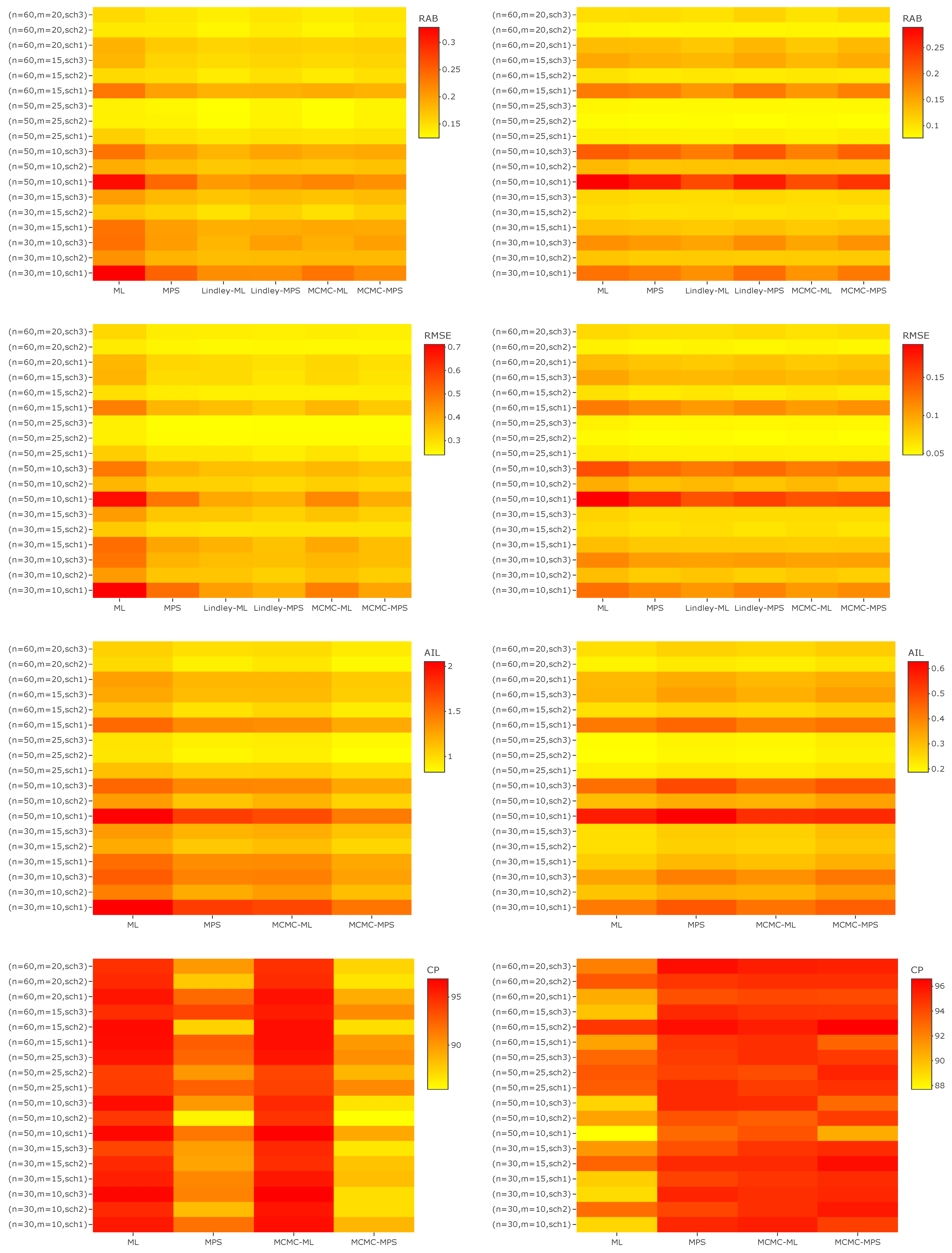
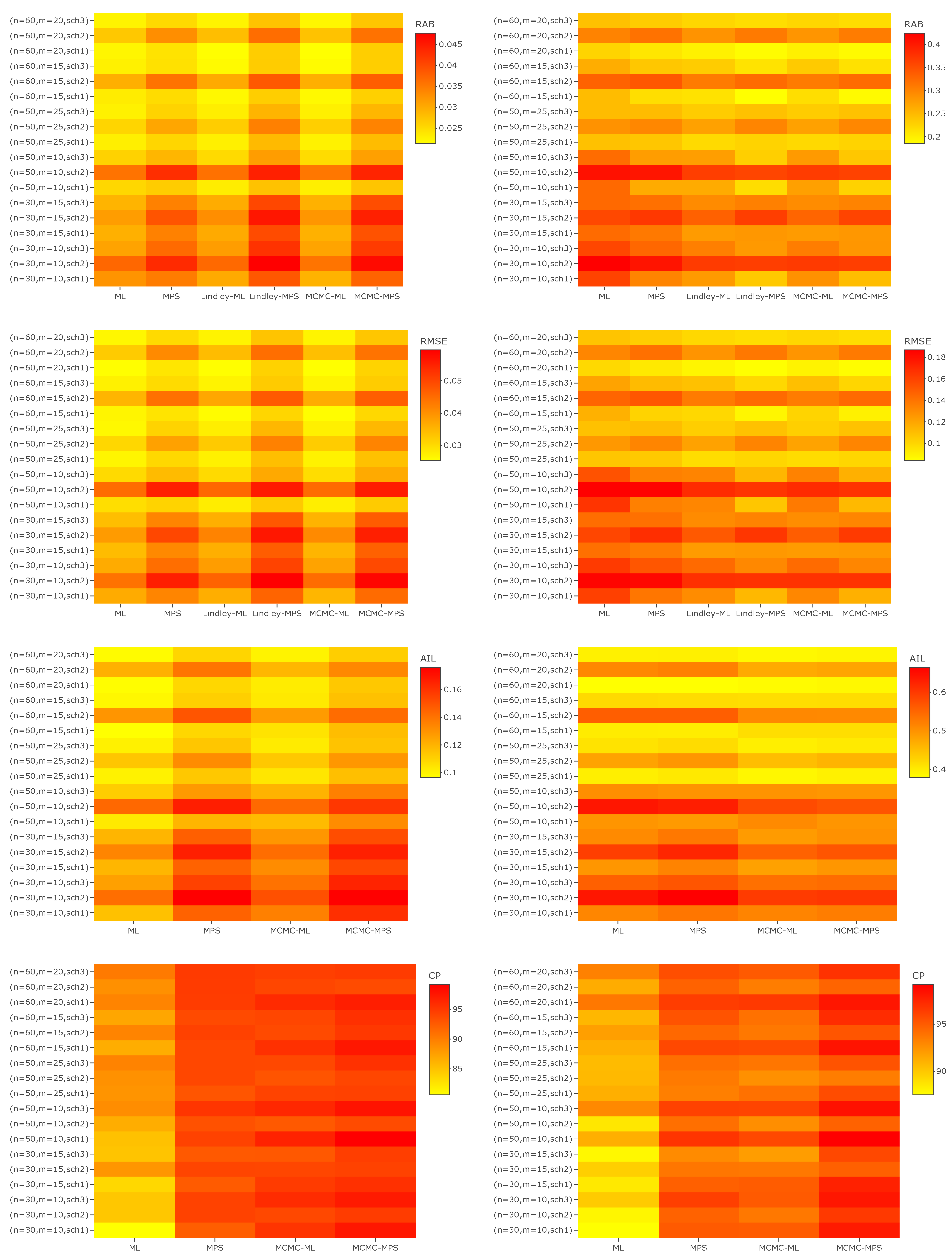
• In most cases, the MPS method performs better in terms of RAB and RMSE than the ML method for a, $\lambda$, and $h\left(t\right)$, especially in the case of small m.
• When n is fixed, the values of RAB, RMSE and AIL become smaller and smaller as m increases for each censoring scheme.
• In most cases, when n and m are fixed, Scheme 2 performs better than the other schemes in terms of RAB, RMSE, and AIL.
• In the majority of cases, LF-based Bayesian estimation using the MCMC technique and Lindley’s approximation performs better than the other approaches for all parameters in terms of RAB.
• In most cases, when comparing the RMSE of a for different approaches, PSF-based Bayesian estimation using Lindley’s approximation performs better than the others, while LF-based Bayesian estimation usually performs better than the other methods for $\lambda$, $R\left(t\right)$, and $h\left(t\right)$ in terms of RMSE.
• For the parameter a, it is observed that PSF-based Bayesian estimation usually provides better estimates than other methods in terms of AIL, while for the parameters $\lambda$ and $R\left(t\right)$ the ML performs better than the other methods in terms of AIL in most cases. The AILs of $h\left(t\right)$ when using the LF-based Bayesian method are usually shorter than the AILs using other methods.
• In terms of CP, the PSF-based Bayesian method usually performs better other approaches for $\lambda$, $R\left(t\right)$, and $h\left(t\right)$. On the other hand, for a the LF-based Bayesian method always surpasses the other methods in terms of CP.
• It can be concluded that the different estimates have asymptotical behaviour with large m. It is observed that the RABs, RMSEs, and AILs all tend to zero as m increases. In the case of small m, it is noted that the MLEs have larger values of RABs, RMSEs, and AILs in most of the cases when compared with the MPSEs and Bayes estimates. On the other hand, it can be seen that the various Bayes estimates perform well with both small and large m when compared with the classical estimates.
• Overall, it can be noted that the MPS method is more accurate than the ML method in the case of a small number of observed failures. On the other hand, the Bayesian estimation methods perform better than the classical methods when there is prior information about the unknown parameters. The Bayesian method requires more computational time than the classical methods. Therefore, in the case of limited time the classical methods are to be preferred over the Bayesian methods. Finally, when no information is available about the unknown parameters and the decision is taken to use non-informative priors, it is advised to use the classical methods in this case, as the acquired estimates can be expected to approximately coincide.

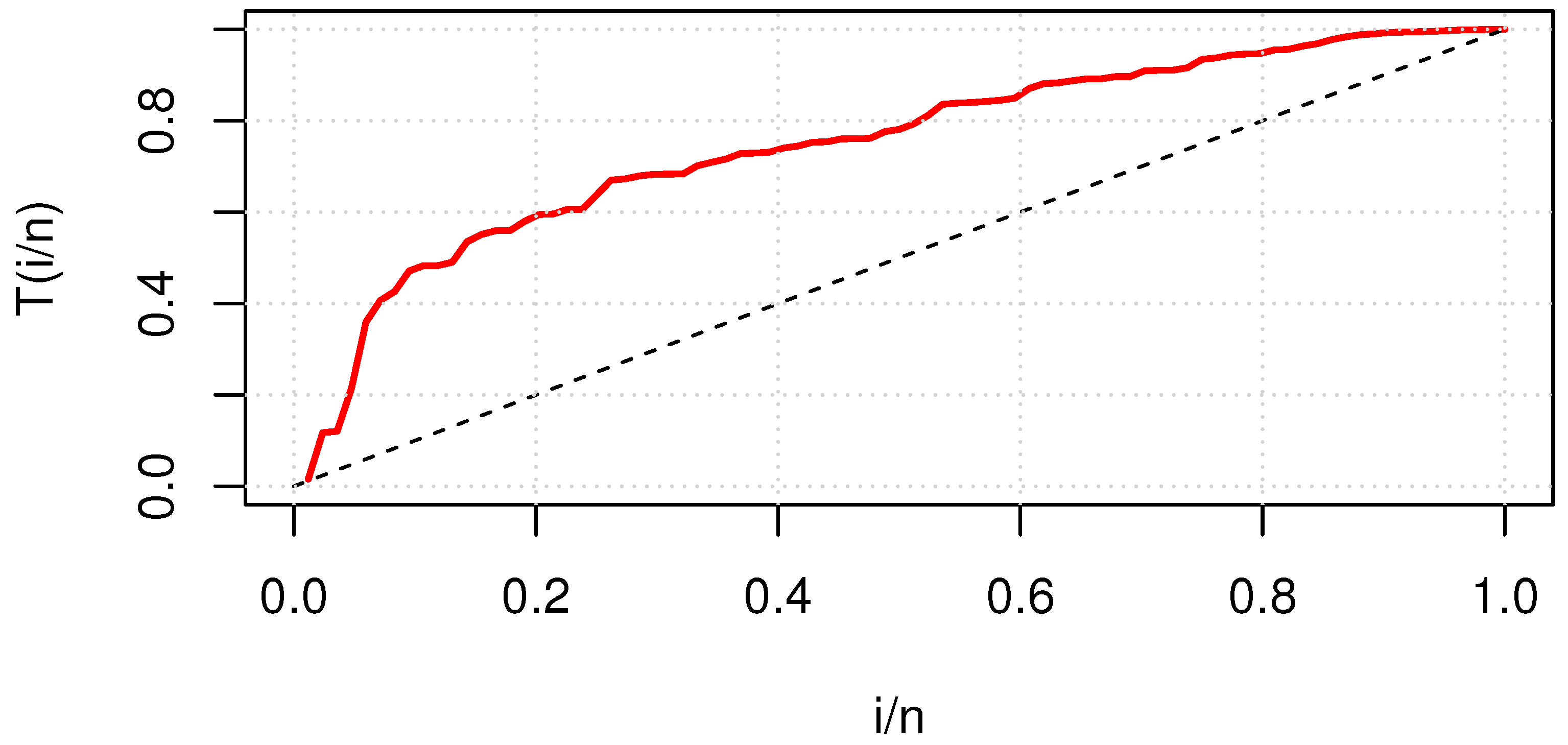
7. Real Data Analysis

In this section, we illustrate the applicability of the suggested estimation methods using two real-life datasets. After checking the suitability of the MKiEx distribution to fit the considered datasets, different censored samples were generated and the point estimates with the associated standard errors (SEs) of the estimates were obtained. The lower bound, upper bound, and length of the ACIs and HPD credible intervals were obtained as well. The point and interval estimates of the RF and HRF were obtained at $t=0.3$. We eliminated the effects of the initial values using the MCMC procedure by discarding the first 2000 iterations from 12,000 MCMC chains. Regarding the choices of the hyperparameters, we followed the method proposed by Kundu [34] and Dey et al. [38] to select the values of $(a_1,b_1)$ and $(a_2,b_2)$ of a and $\lambda$, respectively.

7.1. Failure Times of Aircraft Windshields

These data were reported by Ijaz et al. [39], and represent the uncensored failure times of 84 aircraft windshields. The data values are: 0.040, 0.301, 0.309, 0.557, 0.943, 1.070, 1.124, 1.248, 1.281, 1.281, 1.303, 1.432, 1.480, 1.505, 1.506, 1.568, 1.615, 1.619, 1.652, 1.652, 1.757, 1.866, 1.876, 1.899, 1.911, 1.912, 1.914, 1.981, 2.010, 2.038, 2.085, 2.089, 2.097, 2.135, 2.154, 2.190, 2.194, 2.223, 2.224, 2.229, 2.300, 2.324, 2.385, 2.481, 2.610, 2.625, 2.632, 2.646, 2.661, 2.688, 2.820, 2.890, 2.902, 2.934, 2.962, 2.964, 3.000, 3.000, 3.103, 3.114, 3.117, 3.166, 3.344, 3.376, 3.443, 3.467, 3.478, 3.578, 3.595, 3.699, 3.779, 3.924, 4.035, 4.121, 4.167, 4.240, 4.255, 4.278, 4.305, 4.376, 4.449, 4.485, 4.570, 4.602. To check the suitability of the MKiEx model to fit this dataset, the Kolmogorov–Smirnov (KS) distance based on the MLEs was obtained. The KS = 0.065647 and the associated p-value = 0.8621. These results imply that the MKiEx is an acceptable model to fit the given data. Moreover, Figure 5 displays the TTT plot of the data. According to Barlow and Campo [40], if the curve is concave, this indicates that the hazard rate function is increasing; if this is first convex and afterwards concave, it indicates a bathtub shape for the hazard rate function. This in turn indicates that the data have an increasing failure rate function. Figure 6 shows the histogram with the density curve, estimated CDF, probability–probability (PP), and quantile–quantile (QQ) plots for the complete data. Figure 5 and Figure 6 indicate that the MKiEx distribution is a suitable model to analyze these data. Based on the complete data, the different progressive type-II censored samples shown in

Table 1. Different censored data generated from the first dataset.

m	Censoring Scheme	Generated Samples
10	sch1: (2 × 9, 56)	0.040, 0.301, 0.309, 0.557, 0.943, 1.124, 1.248, 1.281, 1.303, 1.432
30	sch2: (2 × 27, 0 × 3)	0.040, 0.301, 0.309, 0.557, 0.943, 1.070, 1.124, 1.248, 1.281, 1.303, 1.480, 1.615, 1.619, 1.757, 1.866, 1.876, 1.899, 1.912, 2.085, 2.097, 2.154, 2.223, 2.224, 2.324, 2.934, 3.000, 3.117, 3.166, 3.595, 4.305
42	sch3: (1 × 42)	0.040, 0.301, 0.309, 0.557, 1.070, 1.124, 1.248, 1.281, 1.303, 1.432, 1.480, 1.505, 1.568, 1.619, 1.652, 1.757, 1.866, 1.876, 1.899, 1.911, 1.912, 1.981, 2.010, 2.038, 2.135, 2.154, 2.190, 2.223, 2.229, 2.300, 2.324, 2.385, 2.481, 2.625, 2.632, 2.962, 3.117, 3.166, 3.344, 3.443, 3.699, 4.121

were created as.

Table 2. Point estimates (with their SEs) for the first dataset.

sch		ML	MPS	Lindley-ML	Lindley-MPS	MCMC-ML	MCMC-MPS
1	a	1.2206	0.9658	1.4325	0.8454	1.3504	0.9426
		(0.3466)	(0.2977)	(0.2744)	(0.2723)	(0.2387)	(0.1940)
	$\lambda$	0.1294	0.0853	0.1639	0.0623	0.1502	0.0821
		(0.0629)	(0.0585)	(0.0525)	(0.0538)	(0.0391)	(0.0363)
	$R\left(t\right)$	0.9808	0.9710	0.9833	0.9627	0.9819	0.9669
		(0.0126)	(0.0164)	(0.0123)	(0.0141)	(0.0105)	(0.0169)
	$h\left(t\right)$	0.0805	0.0958	0.0710	0.0977	0.0773	0.0992
		(0.0341)	(0.0337)	(0.0328)	(0.0336)	(0.0328)	(0.0365)
2	a	1.7523	1.5726	1.8108	1.4385	1.7857	1.5176
		(0.2382)	(0.2218)	(0.2309)	(0.1767)	(0.1638)	(0.1437)
	$\lambda$	0.2243	0.2143	0.2271	0.2031	0.2253	0.2110
		(0.0185)	(0.0204)	(0.0183)	(0.0170)	(0.0130)	(0.0138)
	$R\left(t\right)$	0.9907	0.9860	0.9902	0.9800	0.9906	0.9830
		(0.0056)	(0.0078)	(0.0056)	(0.0050)	(0.0042)	(0.0066)
	$h\left(t\right)$	0.0566	0.0761	0.0569	0.0969	0.0561	0.0863
		(0.0268)	(0.0326)	(0.0268)	(0.0251)	(0.0195)	(0.0257)
3	a	1.7968	1.6612	1.8294	1.5703	1.8196	1.6282
		(0.2145)	(0.2041)	(0.212)	(0.1827)	(0.1569)	(0.1354)
	$\lambda$	0.2309	0.2262	0.2318	0.2216	0.2317	0.2256
		(0.0146)	(0.0157)	(0.0146)	(0.015)	(0.0106)	(0.0111)
	$R\left(t\right)$	0.9913	0.9879	0.9906	0.9838	0.991	0.9861
		(0.0049)	(0.0064)	(0.0049)	(0.0049)	(0.0037)	(0.0051)
	$h\left(t\right)$	0.0545	0.0695	0.0562	0.0854	0.0549	0.0766
		(0.0244)	(0.0290)	(0.0243)	(0.0243)	(0.0180)	(0.0217)

shows the point estimates and SEs for a, $\lambda$, $R\left(t\right)$, and $h\left(t\right)$ based on the generated samples presented in Table 1. It can be observed from Table 2 that in the case of small m, i.e., $m=10$, the SEs of the estimates of a and $\lambda$ of PSF-based Bayesian estimation using the MCMC method are lower than the SEs using other methods. On the other hand, the SEs of $R\left(t\right)$ and $h\left(t\right)$ using the LF-based Bayesian method are lower than the same values when using the other methods. When $m=30$ and $m=42$ for $\lambda$, $R\left(t\right)$, and $h\left(t\right)$, the SEs using LF-based Bayesian estimation with the MCMC approach are lower than the SEs using the other approaches. The SE of the estimate of a using PSF-based Bayesian estimation with the MCMC method is shorter than the SEs using other methods. In all cases, when the value of m increases, the value of SE for all parameters decreases. Moreover,

Table 3. Interval estimates (with their lengths) for the first dataset.

sch		ML	MPS	MCMC-ML	MCMC-MPS
1	a	(0.5412, 1.9000)	(0.3823, 1.5494)	(0.9035, 1.8212)	(0.5824, 1.3149)
		[1.3588]	[1.1671]	[0.9177]	[0.7325]
	$\lambda$	(0.0062, 0.2526)	(0.0000, 0.2000)	(0.0749, 0.2225)	(0.0209, 0.1550)
		[0.2464]	[0.2000]	[0.1476]	[0.1341]
	$R\left(t\right)$	(0.9561, 1.0000)	(0.9389, 1.0000)	(0.962, 0.9976)	(0.935, 0.9946)
		[0.0439]	[0.0611]	[0.0356]	[0.0596]
	$h\left(t\right)$	(0.0137, 0.1474)	(0.0298, 0.1618)	(0.0215, 0.142)	(0.0346, 0.1733)
		[0.1337]	[0.1320]	[0.1205]	[0.1388]
2	a	(1.2854, 2.2191)	(1.1379, 2.0073)	(1.4706, 2.1054)	(1.2526, 1.8175)
		[0.9337]	[0.8693]	[0.6348]	[0.5649]
	$\lambda$	(0.188, 0.2606)	(0.1743, 0.2543)	(0.1999, 0.2505)	(0.1853, 0.2385)
		[0.0726]	[0.0800]	[0.0506]	[0.0533]
	$R\left(t\right)$	(0.9797, 1.0000)	(0.9707, 1.0000)	(0.982, 0.9971)	(0.9698, 0.9939)
		[0.0203]	[0.0293]	[0.0151]	[0.0241]
	$h\left(t\right)$	(0.0040, 0.1092)	(0.0121, 0.1400)	(0.0228, 0.0960)	(0.0391, 0.1367)
		[0.1052]	[0.1279]	[0.0731]	[0.0976]
3	a	(1.3765, 2.2172)	(1.2612, 2.0612)	(1.5198, 2.1271)	(1.3551, 1.8802)
		[0.8407]	[0.8000]	[0.6074]	[0.5251]
	$\lambda$	(0.2023, 0.2595)	(0.1955, 0.2569)	(0.2126, 0.2542)	(0.2026, 0.2459)
		[0.0572]	[0.0614]	[0.0416]	[0.0432]
	$R\left(t\right)$	(0.9816, 1.0000)	(0.9753, 1.0000)	(0.9836, 0.9971)	(0.9757, 0.9945)
		[0.0184]	[0.0247]	[0.0135]	[0.0188]
	$h\left(t\right)$	(0.0067, 0.1023)	(0.0126, 0.1263)	(0.0239, 0.0908)	(0.038, 0.1195)
		[0.0956]	[0.1138]	[0.0670]	[0.0815]

shows the lower and upper bounds of the ACIs and HPDs. For small m, the lengths of the HPDs are shorter than the ACIs in most cases. For larger sample sizes, the interval length of a when using the PSF-based Bayesian method is shorter than when using the other methods. For the remaining parameters, the LF-based Bayesian method always results in shorter interval lengths comparing to the other methods. Increasing the value of m always decreases the interval length. Figure 7 shows the interval estimates of $R\left(x\right)$ and $h\left(x\right)$ for the third censoring scheme. It can be observed that the lower limits of $R\left(x\right)$ with all methods are closer to 0 when x increases. The HPDs obtained based on both the LF and PSF of $R\left(x\right)$ have good performance when compared with the classical ones. For $h\left(x\right)$, it can be seen that the ACI of MPS and the HPD interval when using PSF are shorter than the intervals obtained based on the other methods. Finally, to check the convergence of the MCMC procedures, using each Markovian chain of a and $\lambda$ after burn-in from the third censoring sample as an example, a trace plot (which provides an essential tool to evaluate how well a chain is mixed) and density plot (which provides a histogram of chains) are shown in Figure 8. These results indicate that the chains converge well and that the burn-in period is suitable to remove the effect of the initial values.

7.2. Number of 1000s of Cycles to Failure for Electrical Appliances

This dataset, which was reported by Lawless [10], represents the complete sample of failure times of sixty cycles for electrical appliances. The data values are 0.014, 0.034, 0.059, 0.061, 0.069, 0.080, 0.123, 0.142, 0.165, 0.210, 0.381, 0.464, 0.479, 0.556, 0.574, 0.839, 0.917, 0.969, 0.991, 1.064, 1.088, 1.091, 1.174, 1.270, 1.275, 1.355, 1.397, 1.477, 1.578, 1.649, 1.702, 1.893, 1.932, 2.001, 2.161, 2.292, 2.326, 2.337, 2.628, 2.785, 2.811, 2.886, 2.993, 3.122, 3.248, 3.715, 3.790, 3.857, 3.912, 4.100, 4.106, 4.116, 4.315, 4.510, 4.580, 5.267, 5.299, 5.583, 6.065, 9.701. To check whether the MKiEx model fits this dataset, we conducted the KS test based on the MLEs. The KS = 0.064269 and the associated p-value = 0.9518. According to these results, the MKiEx is a suitable model to fit the provided data. Figure 9 shows the TTT plot of the data, indicating that the data have a bathtub-shaped failure rate function. Figure 10 shows the histogram with the density curve, estimated CDF, PPm and QQ plots for the complete data. Figure 9 and Figure 10 indicate that the MKiEx distribution is an appropriate model for analyzing the data. Different progressive type-II censored samples were generated using the complete data, as shown in

Table 4. Different censored data generated from the second dataset.

m	Censoring Scheme	Generated Samples
10	sch1: (2 × 9, 32)	0.014, 0.034, 0.059, 0.069, 0.080, 0.123, 0.142, 0.210, 0.464, 0.556
20	sch2: (1 × 19, 21)	0.014, 0.034, 0.059, 0.061, 0.069, 0.080, 0.123, 0.142, 0.165, 0.210, 0.464, 0.556, 0.574, 0.839, 0.991, 1.064, 1.088, 1.270, 1.275, 1.355
30	sch3: (1 × 30)	0.014, 0.034, 0.059, 0.061, 0.069, 0.080, 0.123, 0.142, 0.165, 0.210, 0.381, 0.464, 0.479, 0.556, 0.574, 0.839, 0.969, 0.991, 1.064, 1.270, 1.275, 1.397, 1.578, 1.702, 1.932, 2.292, 2.628, 3.248, 3.912, 4.116

.

Table 5. Point estimates (with their SEs) for the second dataset.

sch		ML	MPS	Lindley-ML	Lindley-MPS	MCMC-ML	MCMC-MPS
1	a	0.6877	0.5762	0.7767	0.5267	0.7271	0.5653
		(0.1876)	(0.1688)	(0.1651)	(0.1614)	(0.1387)	(0.1115)
	$\lambda$	0.2084	0.1311	0.2935	0.1199	0.2423	0.1379
		(0.1543)	(0.1270)	(0.1287)	(0.1265)	(0.1186)	(0.0892)
	$R\left(t\right)$	0.8591	0.8549	0.8569	0.8521	0.8590	0.8508
		(0.0421)	(0.0428)	(0.0420)	(0.0427)	(0.0432)	(0.0462)
	$h\left(t\right)$	0.3591	0.3070	0.4131	0.2851	0.3779	0.3075
		(0.1367)	(0.1238)	(0.1256)	(0.1218)	(0.1257)	(0.1041)
2	a	0.7036	0.6391	0.7479	0.5894	0.7226	0.6323
		(0.1314)	(0.1228)	(0.1237)	(0.1123)	(0.0970)	(0.0857)
	$\lambda$	0.2547	0.2243	0.2816	0.1976	0.2675	0.2262
		(0.0828)	(0.0841)	(0.0783)	(0.0797)	(0.0603)	(0.0606)
	$R\left(t\right)$	0.8452	0.8335	0.8472	0.8233	0.8447	0.8287
		(0.0408)	(0.0418)	(0.0407)	(0.0406)	(0.0358)	(0.0374)
	$h\left(t\right)$	0.4098	0.4012	0.4194	0.3846	0.4149	0.4029
		(0.0865)	(0.0859)	(0.0860)	(0.0843)	(0.0749)	(0.0731)
3	a	0.7150	0.6651	0.7300	0.6258	0.7227	0.6528
		(0.1004)	(0.0952)	(0.0993)	(0.0867)	(0.0698)	(0.0654)
	$\lambda$	0.2967	0.2809	0.3055	0.2748	0.3022	0.2790
		(0.0533)	(0.0555)	(0.0526)	(0.0551)	(0.0396)	(0.0408)
	$R\left(t\right)$	0.8327	0.8200	0.8318	0.8043	0.8320	0.8146
		(0.0419)	(0.0429)	(0.0419)	(0.0400)	(0.0291)	(0.0309)
	$h\left(t\right)$	0.4561	0.4588	0.4573	0.4644	0.4581	0.4596
		(0.0791)	(0.0765)	(0.0791)	(0.0763)	(0.0569)	(0.0550)

shows the point estimates and SEs of a, $\lambda$, $R\left(t\right)$, and $h\left(t\right)$ based on the generated samples presented in Table 4. It can be observed from Table 5 that in the case of small m, i.e., $m=10$, the SEs of the estimates of a, $\lambda$, and $h\left(t\right)$ using PSF-based Bayesian estimation with the MCMC method are lower than the SEs using other methods. On the other hand, the SEs of $R\left(t\right)$ using the LF-based Bayesian method with Lindley’s approximation are lower than the SEs using other methods. When $m=30$ and $m=42$, the SEs using both the LF and PSF Bayesian estimation methods with the MCMC approach are lower than the SEs using the other approaches for all parameters. In all cases, when the value of m increases, the value of SE for all parameters decreases.

Table 6. Interval estimates (with their lengths) for the second dataset.

sch		ML	MPS	MCMC-ML	MCMC-MPS
1	a	(0.3200, 1.0554)	(0.2453, 0.9070)	(0.4783, 1.0092)	(0.3570, 0.7898)
		[0.7354]	[0.6617]	[0.5308]	[0.4329]
	$\lambda$	(0.0000, 0.5108)	(0.0000, 0.3799)	(0.0365, 0.4687)	(0.0058, 0.3122)
		[0.5108]	[0.3799]	[0.4322]	[0.3063]
	$R\left(t\right)$	(0.7767, 0.9416)	(0.7711, 0.9388)	(0.7739, 0.9404)	(0.7587, 0.9364)
		[0.1649]	[0.1677]	[0.1666]	[0.1777]
	$h\left(t\right)$	(0.0910, 0.6271)	(0.0644, 0.5496)	(0.1447, 0.6213)	(0.1249, 0.5134)
		[0.5360]	[0.4852]	[0.4766]	[0.3885]
2	a	(0.4461, 0.9611)	(0.3985, 0.8798)	(0.5417, 0.9116)	(0.4696, 0.7958)
		[0.5150]	[0.4813]	[0.3698]	[0.3262]
	$\lambda$	(0.0924, 0.4169)	(0.0596, 0.3891)	(0.1491, 0.3818)	(0.1105, 0.3443)
		[0.3245]	[0.3295]	[0.2327]	[0.2338]
	$R\left(t\right)$	(0.7652, 0.9251)	(0.7515, 0.9155)	(0.7721, 0.9099)	(0.7533, 0.8976)
		[0.1599]	[0.1640]	[0.1378]	[0.1444]
	$h\left(t\right)$	(0.2403, 0.5794)	(0.2329, 0.5695)	(0.2672, 0.5588)	(0.2639, 0.5485)
		[0.3391]	[0.3366]	[0.2916]	[0.2846]
3	a	(0.5183, 0.9118)	(0.4786, 0.8517)	(0.5887, 0.8609)	(0.5292, 0.7851)
		[0.3935]	[0.3732]	[0.2721]	[0.2559]
	$\lambda$	(0.1921, 0.4012)	(0.1722, 0.3896)	(0.2291, 0.3843)	(0.2001, 0.3586)
		[0.2091]	[0.2174]	[0.1552]	[0.1586]
	$R\left(t\right)$	(0.7506, 0.9148)	(0.7359, 0.9042)	(0.7757, 0.8896)	(0.75, 0.8706)
		[0.1642]	[0.1683]	[0.1139]	[0.1206]
	$h\left(t\right)$	(0.3011, 0.6112)	(0.3089, 0.6086)	(0.3443, 0.5681)	(0.3534, 0.5665)
		[0.3101]	[0.2997]	[0.2238]	[0.2131]

shows the lower and upper bounds of the ACIs and HPDs. For small m, the length of the HPDs based on PSF are shorter than ACIs of both ML and MPS for a, $\lambda$, and $h\left(t\right)$. The ACI using the ML method of $R\left(t\right)$ is the shortest among all methods. For larger sample sizes, the interval lengths of the HPDs are always shorter than the interval lengths of the ACIs when using the ML and MPS methods for all parameters. Increasing the value of m decreases the interval length.

Figure 11 shows the interval estimates of $R\left(x\right)$ and $h\left(x\right)$ for the third censoring scheme. It can be observed that the lower limits of $R\left(x\right)$ with all methods are closer to 0 when x increases. The HPDs obtained based on both the LF and PSF of $R\left(x\right)$ have good performance compared to the real data. For $h\left(x\right)$, it can be seen that the ACIs of the MPS and HPD interval using PSF are shorter than the ACIs of the ML and HPD interval when using LF methods. Finally, using the third censoring sample as an example, we checked the convergence of the MCMC method for each Markovian chain of a and $\lambda$ after burn-in, with the trace plot and density plot shown in Figure 12. These results imply that the chains converge well and that the burn-in period is appropriate for removing the effects of the initial values.

8. Conclusions

In this paper, we have investigated the estimation problems of the modified Kies exponential distribution under a progressive type-II censoring scheme. Two classical estimation methods are used to estimate the unknown parameters of the modified Kies exponential distribution a and $\lambda$, as well as the associated reliability and hazard rate functions, namely, the maximum likelihood and maximum product of spacing. Moreover, Bayesian methods based on the likelihood and product of the spacing functions are used. For the Bayesian methods, we used Lindley’s approximation and the Monte Carlo Markov Chain technique. We obtained the approximate confidence intervals of the maximum likelihood and maximum product of spacing as well as the highest posterior density of the Bayesian method based on the likelihood and the product of the spacing functions. We conducted a simulation study using the modified Kies exponential model. Different sample sizes, parameter values, and censoring schemes were used when performing the simulation study. Finally, two real datasets were examined to show the practicality of the proposed approaches and demonstrate how easy to use and flexible it can be in real-world scenarios. Our numerical outcomes show that the Bayesian methods based on both the likelihood and product of the spacing functions are more accurate than the maximum likelihood and maximum product of the spacing techniques. It is important to mention here that the Bayesian methods require more computational time than the classical methods; therefore, in the case of limited time or no available prior information about the unknown parameters, the classical methods can be preferred over Bayesian methods. As future work, it is of interest to study the behaviour of the presented estimation methods for more general progressive censoring schemes, such as hybrid, general progressive, and adaptive censoring schemes.

References

1. Al-Babtain, A.A.; Shakhatreh, M.K.; Nassar, M.; Afify, A.Z. A new modified Kies family: Properties, estimation under complete and type-II censored samples, and engineering applications. Mathematics 2020, 8, 1345. [Google Scholar] [CrossRef]
2. Aljohani, H.M.; Almetwally, E.M.; Alghamdi, A.S.; Hafez, E. Ranked set sampling with application of modified Kies exponential distribution. Alex. Eng. J. 2021, 60, 4041–4046. [Google Scholar] [CrossRef]
3. Nassar, M.; Alam, F.M.A. Analysis of Modified Kies Exponential Distribution with Constant Stress Partially Accelerated Life Tests under Type-II Censoring. Mathematics 2022, 10, 819. [Google Scholar] [CrossRef]
4. El-Raheem, A.M.A.; Almetwally, E.M.; Mohamed, M.S.; Hafez, E.H. Accelerated life tests for modified Kies exponential lifetime distribution: Binomial removal, transformers turn insulation application and numerical results. AIMS Math. 2021, 6, 5222–5255. [Google Scholar] [CrossRef]
5. Ng, H.K.; Luo, L.; Hu, Y.; Duan, F. Parameter estimation of three-parameter weibull distribution based on progressively type-II censored samples. J. Stat. Comput. Simul. 2012, 82, 1661–1678. [Google Scholar] [CrossRef]
6. Singh, R.; Kumar Singh, S.; Singh, U. Maximum product spacings method for the estimation of parameters of generalized inverted exponential distribution under progressive type II censoring. J. Stat. Manag. Syst. 2016, 19, 219–245. [Google Scholar] [CrossRef]
7. Alshenawy, R.; Al-Alwan, A.; Almetwally, E.M.; Afify, A.Z.; Almongy, H.M. Progressive type-II censoring schemes of extended odd weibull exponential distribution with applications in medicine and engineering. Mathematics 2020, 8, 1679. [Google Scholar] [CrossRef]
8. Lin, Y.J.; Okasha, H.M.; Basheer, A.M.; Lio, Y.L. Bayesian estimation of Marshall Olkin extended inverse Weibull under progressive type II censoring. Qual. Reliab. Eng. Int. 2023, 39, 931–957. [Google Scholar] [CrossRef]
9. Balakrishnan, N.; Cramer, E. The Art of Progressive Censoring: Applications to Reliability and Quality; Springer: Berlin/Heidelberg, Germany, 2016. [Google Scholar]
10. Lawless, J.F. Statistical Models and Methods for Lifetime Data; John Wiley & Sons: Hoboken, NJ, USA, 2003. [Google Scholar]
11. Cheng, R.C.; Amin, N.A. Estimating parameters in continuous univariate distributions with a shifted origin. J. R. Stat. Soc. Ser. B (Methodol.) 1983, 45, 394–403. [Google Scholar] [CrossRef]
12. Ranneby, B. The Maximum Spacing Method. An Estimation Method Related to the Maximum Likelihood Method. Scand. J. Stat. 1984, 11, 93–112. [Google Scholar]
13. Rahman, M.; Pearson, L.M. Estimation in two-parameter exponential distributions. J. Stat. Comput. Simul. 2001, 70, 371–386. [Google Scholar] [CrossRef]
14. Singh, U.; Singh, S.K.; Singh, R.K. A comparative study of traditional estimation methods and maximum product spacings method in generalized inverted exponential distribution. J. Stat. Appl. Probab. 2014, 3, 153–169. [Google Scholar] [CrossRef]
15. Rahman, M.; An, D.; Patwary, M.S. Method of product spacings parameter estimation for beta inverse weibull distribution. Far East J. Theor. Stat. 2016, 52, 1–15. [Google Scholar] [CrossRef]
16. Aruna, C.V. Estimation of Parameters of Lomax Distribution by Using Maximum Product Spacings Method. Int. J. Res. Appl. Sci. Eng. Technol. 2022, 10, 1316–1322. [Google Scholar] [CrossRef]
17. Teimouri, M.; Nadarajah, S. MPS: An R package for modelling shifted families of distributions. Aust. N. Z. J. Stat. 2022, 64, 86–108. [Google Scholar] [CrossRef]
18. Almetwally, E.M.; Jawa, T.M.; Sayed-Ahmed, N.; Park, C.; Zakarya, M.; Dey, S. Analysis of unit-Weibull based on progressive type-II censored with optimal scheme. Alex. Eng. J. 2023, 63, 321–338. [Google Scholar] [CrossRef]
19. Tashkandy, Y.A.; Almetwally, E.M.; Ragab, R.; Gemeay, A.M.; El-Raouf, M.A.; Khosa, S.K.; Hussam, E.; Bakr, M. Statistical inferences for the extended inverse Weibull distribution under progressive type-II censored sample with applications. Alex. Eng. J. 2023, 65, 493–502. [Google Scholar] [CrossRef]
20. DeGroot, M.H.; Schervish, M.J. Probability and Statistics; Pearson Education, Inc.: London, UK, 2019. [Google Scholar]
21. Cohen, A.C. Maximum Likelihood Estimation in the Weibull Distribution Based on Complete and on Censored Samples. Technometrics 1965, 7, 579–588. [Google Scholar] [CrossRef]
22. Casella, G.; Berger, R.L. Statistical Inference; Cengage Learning: Duxbury, CA, USA, 2002. [Google Scholar]
23. Greene, W.H. Econometric Analysis; Prentice Hall: Englewood Cliffs, NJ, USA, 2000. [Google Scholar]
24. Fathi, A.; Farghal, A.W.A.; Soliman, A.A. Bayesian and Non-Bayesian inference for Weibull inverted exponential model under progressive first-failure censoring data. Mathematics 2022, 10, 1648. [Google Scholar] [CrossRef]
25. Eliwa, M.S.; EL-Sagheer, R.M.; El-Essawy, S.H.; Almohaimeed, B.; Alshammari, F.S.; El-Morshedy, M. General entropy with Bayes techniques under Lindley and MCMC for estimating the new Weibull–Pareto parameters: Theory and application. Symmetry 2022, 14, 2395. [Google Scholar] [CrossRef]
26. Dey, S.; Elshahhat, A.; Nassar, M. Analysis of progressive type-II censored gamma distribution. Comput. Stat. 2022, 38, 481–508. [Google Scholar] [CrossRef]
27. Lindley, D.V. Approximate Bayesian methods. Trab. Estad. Y Investig. Oper. 1980, 31, 223–245. [Google Scholar] [CrossRef]
28. Chen, M.H.; Shao, Q.M. Monte Carlo Estimation of Bayesian Credible and HPD Intervals. J. Comput. Graph. Stat. 1998, 8, 69–92. [Google Scholar] [CrossRef]
29. Coolen, F.; Newby, M. A note on the use of the product of spacings in Bayesian inference. KM 1991, 37, 19–32. [Google Scholar]
30. Cohen, A.C.; Whitten, B.J. Parameter Estimation in Reliability and Life SPAN Models; Dekker: Nottingham, UK, 1988. [Google Scholar]
31. Basu, S.; Singh, S.K.; Singh, U. Bayesian inference using product of spacings function for Progressive Hybrid Type-I censoring scheme. Statistics 2017, 52, 345–363. [Google Scholar] [CrossRef]
32. Nassar, M.; Elshahhat, A. Statistical Analysis of Inverse Weibull Constant-Stress Partially Accelerated Life Tests with Adaptive Progressively Type I Censored Data. Mathematics 2023, 11, 370. [Google Scholar] [CrossRef]
33. Balakrishnan, N.; Sandhu, R.A. A Simple Simulational Algorithm for Generating Progressive Type-II Censored Samples. Am. Stat. 1995, 49, 229–230. [Google Scholar] [CrossRef]
34. Kundu, D. Bayesian Inference and Life Testing Plan for the Weibull Distribution in Presence of Progressive Censoring. Technometrics 2008, 50, 144–154. [Google Scholar] [CrossRef]
35. Kundu, D.; Howlader, H. Bayesian inference and prediction of the inverse Weibull distribution for Type-II censored data. Comput. Stat. Data Anal. 2010, 54, 1547–1558. [Google Scholar] [CrossRef]
36. Kundu, D.; Raqab, M.Z. Bayesian inference and prediction of order statistics for a Type-II censored Weibull distribution. J. Stat. Plan. Inference 2012, 142, 41–47. [Google Scholar] [CrossRef]
37. Basu, S.; Singh, S.K.; Singh, U. Estimation of inverse Lindley distribution using product of spacings function for hybrid censored data. Methodol. Comput. Appl. Probab. 2019, 21, 1377–1394. [Google Scholar] [CrossRef]
38. Dey, S.; Dey, T.; Luckett, D.J. Statistical inference for the generalized inverted exponential distribution based on upper record values. Math. Comput. Simul. 2016, 120, 64–78. [Google Scholar] [CrossRef]
39. Ijaz, M.; Mashwani, W.K.; Belhaouari, S.B. A novel family of lifetime distribution with applications to real and simulated data. PLoS ONE 2020, 15, e0238746. [Google Scholar] [CrossRef]
40. Barlow, R.E.; Campo, R.A. Total Time on Test Processes and Applications to Failure Data Analysis; Technical Report; California Univ. Berkeley Operations Research Center: Berkeley, CA, USA, 1975. [Google Scholar]
Figure 1. 3D plot of log-LF for simulated dataset.
Axioms 12 00917 g001
Figure 2. 3D plot of log-PSF for a simulated dataset.
Axioms 12 00917 g002
Figure 3. Heat map for the estimation results of a (left) and λ (right).
Axioms 12 00917 g003
Figure 4. Heat map for the estimation results of R ( t ) (left) and h ( t ) (right).
Axioms 12 00917 g004
Figure 5. TTT plot for the first dataset.
Axioms 12 00917 g005
Figure 6. Histogram of the first dataset with density curve, Estimated CDF, PP plot, and QQ plot.
Axioms 12 00917 g006
Figure 7. Interval estimates of R ( x ) (left) and h ( x ) (right) for the third censoring sample generated from the first dataset: (left) and λ (right).
Axioms 12 00917 g007
Figure 8. Trace and density plots of MCMC draws of a and λ using the LF-based (left) and PSF-based (right) Bayesian estimation methods for the first dataset.
Axioms 12 00917 g008
Figure 9. TTT plot for the second dataset.
Axioms 12 00917 g009
Figure 10. Histogram of the second dataset with density curve, Estimated CDF, PP plot, and QQ plot.
Axioms 12 00917 g010
Figure 11. Interval estimates of R ( x ) (left) and h ( x ) (right) for the third censoring sample generated from the second dataset: (left) and λ (right).
Axioms 12 00917 g011
Figure 12. Trace and density plots of MCMC draws of a and λ using the LF-based (left) and PSF-based (right) Bayesian estimation methods for the second dataset.
Axioms 12 00917 g012