Analysis of the Stress–Strength Model Using Uniform Truncated Negative Binomial Distribution under Progressive Type-II Censoring

Abstract

In this study, we introduce a novel estimation technique for assessing the reliability parameter $R=P(Y<X)$ of the uniform truncated negative binomial distribution (UTNBD) in the context of stress–strength analysis. We base our inferences on the assumption that both the strength (X) and stress (Y) random variables follow a UTNBD with identical first shape and scale parameters. In the presence of a progressive type-II censoring scheme, we employ maximum likelihood, two parametric bootstrap methods, and Bayesian estimation approaches to derive the estimators. Due to the complexity introduced by censoring, the estimators are not available in explicit forms and are instead obtained through numerical approximation techniques. Furthermore, we compute the highest posterior density credible intervals and determine the asymptotic variance-covariance matrix. To assess the performance of our proposed estimators, we conduct a Monte Carlo simulation study and provide a comparative analysis. Finally, we illustrate the practical applicability of our study with an engineering application.

1. Introduction

Due to its relevance in several fields, including engineering, economics, and quality control, and its countless applications to medical and engineering issues in recent years, stress–strength models have drawn the attention of many statisticians for a long time. Stress–strength patterns associated with any system or piece of equipment are often analyzed using stress–strength reliability (SSR) models in the discipline of mechanical engineering. The SSR model evaluates the performance of the system when strength is X and applied stress is Y. The mechanism will malfunction if the applied stress is greater than its capacity. In the present, the SSR model is frequently applied to evaluate the probability that one device will fail before the other in a life testing experiment where X and Y denote the lifetime of two devices. The model will behave as predicted when X surpasses Y, with the SSR model being represented by $R=P\left(Y<X\right)$. In this configuration, it is essential to estimate a component’s reliability characteristics. This helps us assess how effectively a product’s operating procedure works and enables us to take preventative measures to avoid production process hiccups. In a superb monograph published by Kotz et al. [1], the various SSR models created before 2001 were described in detail. Although the improvements for the stress–strength models under complete samples have received a great deal of attention see for instance [2,3,4,5,6,7,8,9,10], much focus has been placed on the situation where the data are record values, see [11,12,13,14,15,16,17].

Censoring occurs in a life-testing experiment when exact lifetimes of items are only known for a portion of their lives and the remaining lifetimes are only known to surpass specific values. Type-I and type-II censoring schemes are the two most widely utilized censoring techniques in the literature. Type-I censoring schemes end experiments after a predetermined amount of time, whereas type-II censoring schemes end experiments after a predetermined number of failures. However, these censoring strategies forbid the removal of units from the test at locations other than the final termination point. A more comprehensive censoring method, termed the progressive censoring scheme, which permits the removal of units from the test at points other than the eventual termination point, serves this goal. It can be described as follows: consider a scenario where n units are tested, but only m of the failures are completely apparent. At the time of the first failure, $X_{1:m:n}$, one of the surviving units $R_1^{\ast }$ is randomly selected and eliminated from the remaining $(n-1)$ units. When a second failure, $X_{2:m:n}$, is discovered, $R_2^{\ast }$ of the surviving units, just as in the first example, are randomly selected and deleted from the remaining $\left(n-2-R_1^{\ast }\right)$ units. At the mth stage, where $X_{m:m:n}$ is seen, all of the $R_m^{\ast }$ remaining surviving units are finally eliminated from the experiment. This process of obtaining the censored sample of size m is known as progressive type-II censored (PTIIC) sample with censoring scheme $\left(R_1^{\ast },R_2^{\ast },\dots ,R_m^{\ast }\right)$. For more details, we refer the reader to Balakrishnan and Sandhu [18]. The issue of estimating the SSR parameter for various sampling schemes and distributions for X and Y has been the subject of extensive research by several statistical scholars including [19,20,21,22].

The uniform truncated negative binomial distribution is frequently used in reliability analysis. When contrasted to the well-known families of distributions, such as Weibull, gamma, generalized exponential, etc., it can occasionally be considered as a good substitute. Kamel et al. [23] studied some of its statistical and reliability characteristics, including the shape behavior of the density and hazard rate functions, the mean residual life and moment generating functions, the limiting distribution of sample extremes, quantiles, kurtosis, skewness, entropies, and stochastic orderings, and they first proposed the concept of UTNBD. They also conducted a straightforward investigation of maximum likelihood estimates using censored data from actual observations. UTNBD is examined in this article as part of a stress–strength study related to any system in the presence of a progressive type-II censoring scheme. The probability density function (PDF) and cumulative distribution function (CDF) of UTNBD are provided by

$$f\left(x;\alpha ,\theta ,\lambda \right)=\frac{\lambda {\alpha }^{\lambda }\left(1-\alpha \right)}{\theta \left(1-{\alpha }^{\lambda }\right)}{\left(\alpha +\frac{1-\alpha }{\theta }x\right)}^{-\left(\lambda +1\right)},\alpha ,\lambda >0,0<x<\theta ,$$

(1)

and

$$F\left(x;\alpha ,\theta ,\lambda \right)=1-\frac{{\alpha }^{\lambda }}{\left(1-{\alpha }^{\lambda }\right)}\left[{\left(\alpha +\frac{1-\alpha }{\theta }x\right)}^{-\lambda }-1\right],\alpha ,\lambda >0,0<x<\theta ,$$

(2)

where $\alpha$ and $\lambda$ are the shape parameters and $\theta$ is the scale parameter. It has sub-models including the uniform and Marshall–Olkin extended uniform (MOEU) distributions: when $\alpha \to 1$, then $UTNB\left(\alpha ,\theta ,\lambda \right)$ reduce to $U\left(0,\theta \right),$ and when $\lambda \to 1$, the MOEU distribution is obtained. Let X and Y represent the two independent strength–stress random variables discovered from $UTNB\left(\alpha ,\theta ,{\lambda }_1\right)$ and $UTNB\left(\alpha ,\theta ,{\lambda }_2\right)$, respectively. The SSR parameter is assessed with the presumption that models have the same first-shape and scale parameters but distinct second-shape parameters, i.e., $X\sim UTNB\left(\alpha ,\theta ,{\lambda }_1\right)$ and $Y\sim UTNB\left(\alpha ,\theta ,{\lambda }_2\right)$. In light of this, the SSR parameter R is

$$\begin{array}{ccc}\hfill R& =& P\left(Y<X\right)={\int }_0^{\theta }P\left(X>Y|Y=y\right)f_2\left(y;\alpha ,\theta ,{\lambda }_2\right)dy\hfill \\ & =& {\int }_0^{\theta }\overline{F_1}\left(y;\alpha ,\theta ,{\lambda }_1\right)f_2\left(y;\alpha ,\theta ,{\lambda }_2\right)dy\hfill \\ & =& \frac{{\lambda }_2-{\alpha }^{{\lambda }_1}\left[{\lambda }_1+{\lambda }_2-{\lambda }_1{\alpha }^{{\lambda }_2}\right]}{\left({\lambda }_1+{\lambda }_2\right)\left({\alpha }^{{\lambda }_1}-1\right)\left({\alpha }^{{\lambda }_2}-1\right)}\hfill \\ & =& \Omega \left(\alpha ,{\lambda }_1,{\lambda }_2\right).\hfill \end{array}$$

(3)

The article’s general structure is as follows: The maximum likelihood estimates and asymptotic confidence intervals are covered in Section 2. In Section 3, two parametric bootstrap techniques are suggested. Section 4 examines estimate methods in a Bayesian framework. A simulation study is carried out to compare the suggested techniques in Section 5. A case study using actual data is given in Section 6 to show how the suggested inference processes might be used. In Section 7, a summary of the findings is presented.

2. Maximum Likelihood Estimation

Maximum likelihood estimation (MLE) is a well-liked method for parameter estimation in statistical models. It is a technique for determining statistical models’ unidentified parameters by using test data. The principle behind MLE is that the collection of parameter values that maximizes the probability of obtaining the observed data is the most likely value of an unknown parameter. MLE is a well-known and frequently used method because it provides a straightforward way to estimate the attributes of a population given a sample in many scientific fields. The fact that it is straightforward to apply computationally is an additional advantage. Let us assume that $x_{1:m_1:n_1},x_{2:m_1:n_1},\dots ,x_{m_1:m_1:n_1}$ and $y_{1:m_2:n_2},y_{2:m_2:n_2},\dots ,y_{m_2:m_2:n_2}$ are two PTIIC samples of strength X and stress Y under the schemes $\left(n_1,m_1,S_1,S_2,\dots ,S_{m_1}\right)$ and $\left(n_2,m_2,T_1,T_2,\dots ,T_{m_2}\right),$, respectively. Then, in this reliability scheme, the likelihood function (LF) of the observed samples is given by (see [15])

$$\begin{array}{ccc}\hfill L(\alpha ,\theta ,{\lambda }_1,{\lambda }_2|\underline{x},\underline{y})& =& C\prod _{i=1}^{m_1}f\left(x_i;\alpha ,\theta ,{\lambda }_1\right){\left[1-F\left(x_i;\alpha ,\theta ,{\lambda }_1\right)\right]}^{S_i}\hfill \\ & & \times \prod _{j=1}^{m_2}f\left(y_j;\alpha ,\theta ,{\lambda }_2\right){\left[1-F\left(y_j;\alpha ,\theta ,{\lambda }_2\right)\right]}^{T_j},\hfill \end{array}$$

(4)

where $x_i=$$x_{i:m_1:n_1}$ and $y_j=y_{j:m_2:n_2}$ to reduce the notation’s complexity, and

$$\begin{array}{ccc}\hfill C& =& C_S{C}_T,\hfill \\ \hfill C_S& =& n_1\left(n_1-1-S_1\right)\left(n_1-2-S_1-S_2\right)\dots \left(n_1-m_1-S_1-\dots -S_{m_1-1}\right),\hfill \\ \hfill C_T& =& n_2\left(n_2-1-T_1\right)\left(n_2-2-T_1-T_2\right)\dots \left(n_2-m_2-T_1-\dots -T_{m_2-1}\right),\hfill \end{array}$$

both equally

$$\begin{array}{ccc}\hfill L(\alpha ,\theta ,{\lambda }_1,{\lambda }_2)& \propto & {\lambda }_1^{m_1}{\lambda }_2^{m_2}{\left(\frac{1-\alpha }{\theta }\right)}^{m_1+m_2}{\left(\frac{{\alpha }^{{\lambda }_1}}{1-{\alpha }^{{\lambda }_1}}\right)}^{m_1}{\left(\frac{{\alpha }^{{\lambda }_2}}{1-{\alpha }^{{\lambda }_2}}\right)}^{m_2}\hfill \\ & & \times exp\left\{-\left({\lambda }_1+1\right)\sum _{i=1}^{m_1}ln\left(\alpha +\frac{1-\alpha }{\theta }{x}_i\right)-\left({\lambda }_2+1\right)\sum _{j=1}^{m_2}ln\left(\alpha +\frac{1-\alpha }{\theta }{y}_j\right)\right\}\hfill \\ & & \times exp\left\{\sum _{i=1}^{m_1}{S}_{i}ln\left(\frac{{\alpha }^{{\lambda }_1}}{1-{\alpha }^{{\lambda }_1}}\right)+\sum _{i=1}^{m_1}{S}_{i}ln\left[{\left(\alpha +\frac{1-\alpha }{\theta }{x}_i\right)}^{-{\lambda }_1}-1\right]\right\}\hfill \\ & & \times exp\left\{\sum _{j=1}^{m_2}{T}_{i}ln\left(\frac{{\alpha }^{{\lambda }_2}}{1-{\alpha }^{{\lambda }_2}}\right)+\sum _{j=1}^{m_2}{T}_{i}ln\left[{\left(\alpha +\frac{1-\alpha }{\theta }{y}_j\right)}^{-{\lambda }_2}-1\right]\right\}.\hfill \end{array}$$

(5)

Consequently, the LF (5) natural logarithm without constant additive terms is written as

$$\begin{array}{ccc}\hfill \ell (\alpha ,\theta ,{\lambda }_1,{\lambda }_2)& \propto & m_{1}ln{\lambda }_1+m_{2}ln{\lambda }_2+\left(m_1+m_2\right)ln\left(\frac{1-\alpha }{\theta }\right)\hfill \\ & & +\left(m_1+\sum _{i=1}^{m_1}{S}_i\right)ln\left(\frac{{\alpha }^{{\lambda }_1}}{1-{\alpha }^{{\lambda }_1}}\right)+\left(m_2+\sum _{j=1}^{m_2}{T}_i\right)ln\left(\frac{{\alpha }^{{\lambda }_2}}{1-{\alpha }^{{\lambda }_2}}\right)\hfill \\ & & -\left({\lambda }_1+1\right)\sum _{i=1}^{m_1}ln\left(\alpha +\frac{1-\alpha }{\theta }{x}_i\right)+\sum _{i=1}^{m_1}{S}_{i}ln\left[{\left(\alpha +\frac{1-\alpha }{\theta }{x}_i\right)}^{-{\lambda }_1}-1\right]\hfill \\ & & -\left({\lambda }_2+1\right)\sum _{j=1}^{m_2}ln\left(\alpha +\frac{1-\alpha }{\theta }{y}_j\right)+\sum _{j=1}^{m_2}{T}_{i}ln\left[{\left(\alpha +\frac{1-\alpha }{\theta }{y}_j\right)}^{-{\lambda }_2}-1\right].\hfill \end{array}$$

(6)

Moreover, $\theta$ is a known common scale parameter. The MLEs of the parameters $\alpha ,$${\lambda }_1$, and ${\lambda }_2$ are calculated by differentiating the previously mentioned expression (6) with regard to the parameters ($\alpha ,$${\lambda }_1$, and ${\lambda }_2$) and equating it to zero. There are the likelihood formulas listed below

$$\begin{array}{ccc}\hfill \frac{\partial \ell (\alpha ,\theta ,{\lambda }_1,{\lambda }_2)}{\partial \alpha }& =& \frac{m_1+m_2}{\left(1-\alpha \right)}+\left(m_1+\sum _{i=1}^{m_1}{S}_i\right)\frac{{\lambda }_1}{\alpha \left(1-{\alpha }^{{\lambda }_1}\right)}+\left(m_2+\sum _{j=1}^{m_2}{T}_i\right)\frac{{\lambda }_2}{\alpha \left(1-{\alpha }^{{\lambda }_2}\right)}\hfill \\ & & -\sum _{i=1}^{m_1}{S}_i\frac{{\lambda }_1\left(1-\frac{x_i}{\theta }\right){\left(\alpha +\frac{1-\alpha }{\theta }{x}_i\right)}^{-\left({\lambda }_1+1\right)}}{{\left(\alpha +\frac{1-\alpha }{\theta }{x}_i\right)}^{-{\lambda }_1}-1}-\sum _{j=1}^{m_2}{T}_i\frac{{\lambda }_2(1-\frac{y_j}{\theta }){\left(\alpha +\frac{1-\alpha }{\theta }{y}_j\right)}^{-\left({\lambda }_2+1\right)}}{{\left(\alpha +\frac{1-\alpha }{\theta }{y}_j\right)}^{-{\lambda }_2}-1}\hfill \\ & & -\left({\lambda }_1+1\right)\sum _{i=1}^{m_1}\frac{1-\frac{x_i}{\theta }}{\left(\alpha +\frac{1-\alpha }{\theta }{x}_i\right)}-\left({\lambda }_2+1\right)\sum _{j=1}^{m_2}\frac{1-\frac{y_j}{\theta }}{\left(\alpha +\frac{1-\alpha }{\theta }{y}_j\right)}\hfill \end{array}$$

(7)

$$\begin{array}{ccc}\hfill \frac{\partial \ell (\alpha ,\theta ,{\lambda }_1,{\lambda }_2)}{\partial {\lambda }_1}& =& \frac{m_1}{{\lambda }_1}+\left(m_1+\sum _{i=1}^{m_1}{S}_i\right)\left(\frac{ln\alpha }{1-{\alpha }^{{\lambda }_1}}\right)-\sum _{i=1}^{m_1}ln\left(\alpha +\frac{1-\alpha }{\theta }{x}_i\right)\hfill \\ & & -\sum _{i=1}^{m_1}{S}_i\frac{{\left(\alpha +\frac{1-\alpha }{\theta }{x}_i\right)}^{-{\lambda }_1}ln\left(\alpha +\frac{1-\alpha }{\theta }{x}_i\right)}{{\left(\alpha +\frac{1-\alpha }{\theta }{x}_i\right)}^{-{\lambda }_1}-1},\hfill \end{array}$$

(8)

and

$$\begin{array}{ccc}\hfill \frac{\partial \ell (\alpha ,\theta ,{\lambda }_1,{\lambda }_2)}{\partial {\lambda }_2}& =& \frac{m_2}{{\lambda }_2}+\left(m_2+\sum _{j=1}^{m_2}{T}_i\right)\left(\frac{ln\alpha }{1-{\alpha }^{{\lambda }_2}}\right)-\sum _{j=1}^{m_2}ln\left(\alpha +\frac{1-\alpha }{\theta }{y}_j\right)\hfill \\ & & -\sum _{j=1}^{m_2}{T}_i\frac{{\left(\alpha +\frac{1-\alpha }{\theta }{y}_j\right)}^{-{\lambda }_2}ln\left(\alpha +\frac{1-\alpha }{\theta }{y}_j\right)}{{\left(\alpha +\frac{1-\alpha }{\theta }{y}_j\right)}^{-{\lambda }_2}-1}.\hfill \end{array}$$

(9)

To obtain the MLEs of the parameters, Equations (7)–(9) are simultaneously solved. Unfortunately, the aforementioned issues cannot be solved analytically. As a result, MLEs can be assessed using any numerical iterative technique. In this case, a non-linear maximization method was used to obtain MLEs (see [24]). By considering the MLEs’ invariance property and substituting their estimates for the parameters as given in the following, it is possible to create the MLE of R, denoted by ${\widehat{R}}_{ML}$:

$$\begin{array}{ccc}\hfill {\widehat{R}}_{ML}& =& \frac{{\widehat{\lambda }}_2-{\widehat{\alpha }}^{{\widehat{\lambda }}_1}\left[{\widehat{\lambda }}_1+{\widehat{\lambda }}_2-{\widehat{\lambda }}_1{\widehat{\alpha }}^{{\widehat{\lambda }}_2}\right]}{\left({\widehat{\lambda }}_1+{\widehat{\lambda }}_2\right)\left({\widehat{\alpha }}^{{\widehat{\lambda }}_1}-1\right)\left({\widehat{\alpha }}^{{\widehat{\lambda }}_2}-1\right)}\hfill \\ & =& \Omega \left(\widehat{\alpha },{\widehat{\lambda }}_1,{\widehat{\lambda }}_2\right).\hfill \end{array}$$

(10)

Asymptotic Confidence Interval

Even though Equation (3)’s precise expression for R has an explicit form, determining its exact distribution is difficult. The asymptotic distribution of R has been considered in order to produce an asymptotic confidence interval (ACI) for R. We were able to determine the asymptotic distribution of $\vartheta =\left(\alpha ,{\lambda }_1,{\lambda }_2\right)$ in this instance based on the asymptotic properties and general state of MLEs (see Casella and Berger [25]). The parameter’s asymptotic distribution often corresponds to the large sample’s normal distribution, i.e,

$$\widehat{\vartheta }-\vartheta \sim N\left(0,\frac{1}{I\left(\widehat{\vartheta }\right)}\right),$$

(11)

where $I\left(\widehat{\vartheta }\right)$ is the observed Fisher information matrix which can be expressed as

$$I\left(\widehat{\vartheta }\right)=\left(\begin{array}{ccc}{\Lambda }_{11}& {\Lambda }_{12}& {\Lambda }_{13}\\ {\Lambda }_{21}& {\Lambda }_{22}& {\Lambda }_{23}\\ {\Lambda }_{31}& {\Lambda }_{32}& {\Lambda }_{33}\end{array}\right)=E{\left(\begin{array}{ccc}-{\ell }_{\alpha \alpha }& -{\ell }_{\alpha {\lambda }_1}& -{\ell }_{\alpha {\lambda }_2}\\ -{\ell }_{{\lambda }_1\alpha }& -{\ell }_{{\lambda }_1{\lambda }_1}& -{\ell }_{{\lambda }_1{\lambda }_2}\\ -{\ell }_{{\lambda }_2\alpha }& -{\ell }_{{\lambda }_2{\lambda }_1}& -{\ell }_{{\lambda }_2{\lambda }_2}\end{array}\right)}_{\downarrow \left(\widehat{\vartheta }\right)}.$$

(12)

It is obvious that in order to calculate R’s asymptotic confidence interval, the variance must be known. The delta approach from Xu and Long [26] is employed for this purpose. The delta method is a statistical technique to derive an approximate probability distribution for a function of an asymptotically normal estimator using the Taylor series approximation. According to the delta method, the variance of R can be expressed as the following

$$\begin{array}{ccc}\hfill {\sigma }_{\widehat{R}}^2& =& {\left(\frac{\partial R}{\partial \alpha }\right)}^2{\Lambda }_{11}^{-1}+{\left(\frac{\partial R}{\partial {\lambda }_1}\right)}^2{\Lambda }_{22}^{-1}+{\left(\frac{\partial R}{\partial {\lambda }_2}\right)}^2{\Lambda }_{33}^{-1}+2\left(\frac{\partial R}{\partial \alpha }\right)\left(\frac{\partial R}{\partial {\lambda }_1}\right){\Lambda }_{12}^{-1},\hfill \\ & & +2\left(\frac{\partial R}{\partial \alpha }\right)\left(\frac{\partial R}{\partial {\lambda }_2}\right){\Lambda }_{13}^{-1}+2\left(\frac{\partial R}{\partial {\lambda }_1}\right)\left(\frac{\partial R}{\partial {\lambda }_2}\right){\Lambda }_{23}^{-1}.\hfill \end{array}$$

(13)

Thus, it is straightforward to construct the first partial derivatives listed in (13). According to Slutsky’s theorem, it is easy to verify that

$$z_R=\frac{{\widehat{R}}_{ML}-R}{\sqrt{{\sigma }_{\widehat{R}}^2}}\to N\left(0,1\right).$$

(14)

As a result, the two-sided $100(1-\delta )\%$ approximate confidence intervals (ACIs) for R are provided by

$$\left[{\widehat{R}}_{ML}-z_{\frac{\delta }{2}}\sqrt{{\sigma }_{\widehat{R}}^2},{\widehat{R}}_{ML}+z_{\frac{\delta }{2}}\sqrt{{\sigma }_{\widehat{R}}^2}\right].$$

(15)

3. Parametric Bootstrap

Normal approximations perform effectively when the proper sample size is large, as mentioned in the previous section. A tiny sample size, however, does not fall within the assumption of normality. In this situation, confidence intervals can be approximated more accurately using resampling techniques such as the bootstrap. Due to its capacity to offer a strong and trustworthy method of evaluating the accuracy of a certain model, bootstrapping has grown in popularity in recent years. Bootstrapping entails resampling data from a population in order to estimate the true mean and variance of the population more precisely. Using this procedure, researchers may more accurately evaluate a model’s correctness. Additionally, the bootstrapping results are examined for potential sources of bias and volatility. Researchers can find possible areas for model development by repeatedly resampling the data. This is very helpful when using the model for prediction. Particularly for small samples, smoothing/bootstrap approaches are used to produce more precise confidence intervals. Two bootstrap resampling methods are suggested to estimate confidence intervals for the SSR parameter in this section.

3.1. Percentile Bootstrap

Efron [27] was the first to establish the bootstrap process (see Davison and Hinkley [28] for further information). In this part, we explore the identical techniques outlined in DiCiccio and Efron [29] in order to obtain a more often-used confidence interval of R. The percentile bootstrap (BP) is described by the following algorithm:

• Create random sample sets $x_{1:m_1:n_1},x_{2:m_1:n_1},\dots ,x_{m_1:m_1:n_1}$ and $y_{1:m_2:n_2},y_{2:m_2:n_2},\dots ,$$y_{m_2:m_2:n_2}$ from $UTNB\left(\alpha ,{\theta }_0,{\lambda }_1\right)$ and $UTNB\left(\alpha ,{\theta }_0,{\lambda }_2\right)$ with $\left(n_1,m_1,S_1,S_2,\dots ,S_{m_1}\right)$ and $(n_2,m_2,$$T_1,$$T_2,$$\dots ,$$T_{m_2}),$, respectively. Determine the MLEs of $\widehat{\alpha },$${\widehat{\lambda }}_1$ and ${\widehat{\lambda }}_2$.
• Use $\widehat{\alpha },$${\widehat{\lambda }}_1$ and ${\widehat{\lambda }}_2$ to generate independent bootstrap samples $x_{1:m_1:n_1}^{\ast },x_{2:m_1:n_1}^{\ast },\dots ,x_{m_1:m_1:n_1}^{\ast }$ and $y_{1:m_2:n_2}^{\ast },y_{2:m_2:n_2}^{\ast },\dots ,y_{m_2:m_2:n_2}^{\ast }$ from $UTNB\left(\widehat{\alpha },{\theta }_0,{\widehat{\lambda }}_1\right)$ and $UTNB\left(\widehat{\alpha },{\theta }_0,{\widehat{\lambda }}_2\right)$ with $\left(n_1,m_1,S_1,S_2,\dots ,S_{m_1}\right)$ and $\left(n_2,m_2,T_1,T_2,\dots ,T_{m_2}\right),$, respectively. Compute the MLEs of unknown parameters based on the bootstrap samples, represented by ${\widehat{\alpha }}^{\ast },$${\widehat{\lambda }}_1^{\ast }$ and ${\widehat{\lambda }}_2^{\ast }$.
• Determine the bootstrap estimate of R in (10), then denote it with the symbol ${\widehat{R}}^{\ast }$.
• Repeat Steps 2 and 3 N times and obtain the ordered value ${\widehat{R}}_{\left(1\right)}^{\ast }\le {\widehat{R}}_{\left(2\right)}^{\ast }\le \dots \le {\widehat{R}}_{\left(N\right)}^{\ast }$.
• The $100(1-\delta )\%$ BP confidence interval of R is given by

  $$\left({\widehat{R}}_{BP}\left[N\left(\frac{\delta }{2}\right)\right],{\widehat{R}}_{BP}\left[N\left(1-\frac{\delta }{2}\right)\right]\right).$$

3.2. Bootstrap-t

The bootstrap-t (BT) approach, as explained by Efron and Tibshirani [30], enables the determination of the confidence interval for the parameters of interest when the sample size is small. BT confidence intervals with parametric data can be produced using the next algorithm.

1–3.

Similar to the BP algorithm mentioned above.

4.

Determine the forthcoming statistics:

$${\Psi }_R^{\ast }=\frac{\left({\widehat{R}}^{\ast }-\widehat{R}\right)}{\sqrt{{\sigma }_{\widehat{R}}^2}}.$$

5.

Repeat Steps (2) through (4) N times.

6.

Assume that $G\left(z\right)=P\left({\Psi }_R^{\ast }\le z\right)$ is the CDF of ${\Psi }_R^{\ast }$. Define ${\widehat{R}}_{BT}\left(z\right)={\widehat{R}}^{\ast }+\sqrt{{\sigma }_{\widehat{R}}^2}{G}^{-1}\left(z\right)$. The approximate $100(1-\delta )\%$ BT confidence interval of R is given by

$$\left({\widehat{R}}_{BT}\left[N\left(\frac{\delta }{2}\right)\right],{\widehat{R}}_{BT}\left[N\left(1-\frac{\delta }{2}\right)\right]\right).$$

4. Bayesian Estimation Using MCMC

Due to its capacity to take into account previous information, Bayesian estimation has a number of benefits over conventional maximum likelihood estimation methods. Additionally, it is able to provide an assessment of the level of uncertainty surrounding each parameter. Bayesian estimation is becoming common in a variety of applications, including signal processing, machine learning, artificial intelligence, and therapeutic protocols, due to its many benefits. For instance, Bayesian estimation can be used to find the parameters of a linear system given a series of observations. It is possible to utilize it in machine learning to identify the best plausible theory given a set of facts. Similar to this, it can be applied to artificial intelligence to forecast an event’s result given a collection of circumstances. It can also be used in the medical field to predict the outcome of using one of the therapeutic protocols for a particular disease in light of a group of limited side effects.

The proper selection of priors for the parameters is necessary for Bayesian deduction. According to Arnold and Press [31], it is obvious that one cannot claim that one prior is superior to all others from a strictly Bayesian perspective. One must presumably accept their own subjective priors and all of their imperfections. However, using informative priors, which are undoubtedly favored over all other options, is preferable if we have sufficient knowledge of the parameter(s). Otherwise, utilizing nondescriptive or ambiguous priors may be appropriate; for further information, see Uppadhyay et al. [32]. According to Kundu and Howlader [33], the family of gamma distributions is recognized to be straightforward and adaptable enough to accommodate a wide range of the experimenter’s preexisting views. Consider a situation where the unknown parameters $\alpha ,$${\lambda }_1$ and ${\lambda }_2$ have conjugate gamma priors and are stochastically independent distributed, i.e., $\alpha \sim gamma\left(a_1,b_1\right)$, ${\lambda }_1\sim gamma\left(a_2,b_2\right)$ and ${\lambda }_2\sim gamma\left(a_3,b_3\right)$ respectively. Thus, the combined prior density of $\alpha ,$${\lambda }_1$ and ${\lambda }_2$ can be expressed as follows

$$\pi (\alpha ,{\lambda }_1,{\lambda }_2)\propto {\alpha }^{a_1-1}{\lambda }_1^{a_2-1}{\lambda }_2^{a_3-1}{e}^{-\left(b_1\alpha +b_2{\lambda }_1+b_3{\lambda }_2\right)},a_i,b_i>0,i=1,2,3.$$

(16)

The joint posterior distribution ${\pi }^{\ast }(\alpha ,{\lambda }_1,{\lambda }_2|\underline{x},\underline{y})={\pi }^{\ast }\left(\vartheta \right)$ can therefore be obtained by combining Equations (5) and (16), the resulting expression is provided by

$$\begin{array}{ccc}\hfill {\pi }^{\ast }\left(\vartheta \right)& \propto & {\alpha }^{a_1-1}{\lambda }_1^{m_1+a_2-1}{\lambda }_2^{m_2+a_3-1}{e}^{-b_1\alpha }exp\left\{-{\lambda }_1\left(b_2+\sum _{i=1}^{m_1}ln\left(\alpha +\frac{1-\alpha }{\theta }{x}_i\right)\right)\right\}\hfill \\ & & \times exp\left\{-{\lambda }_2\left(b_3+\sum _{j=1}^{m_2}ln\left(\alpha +\frac{1-\alpha }{\theta }{y}_j\right)\right)\right\}\prod _{i=1}^{m_1}\frac{\left(1-\alpha \right){\alpha }^{{\lambda }_1}}{\theta \left(1-{\alpha }^{{\lambda }_1}\right)}{\left(\alpha +\frac{1-\alpha }{\theta }{x}_i\right)}^{-1}\hfill \\ & & \times \prod _{j=1}^{m_2}\frac{\left(1-\alpha \right){\alpha }^{{\lambda }_2}}{\theta \left(1-{\alpha }^{{\lambda }_2}\right)}{\left(\alpha +\frac{1-\alpha }{\theta }{y}_j\right)}^{-1}\prod _{i=1}^{m_1}{\left(\frac{{\alpha }^{{\lambda }_1}}{1-{\alpha }^{{\lambda }_1}}\left[{\left(\alpha +\frac{1-\alpha }{\theta }{x}_i\right)}^{-{\lambda }_1}-1\right]\right)}^{S_i}\hfill \\ & & \times \prod _{j=1}^{m_2}{\left(\frac{{\alpha }^{{\lambda }_2}}{1-{\alpha }^{{\lambda }_2}}\left[{\left(\alpha +\frac{1-\alpha }{\theta }{y}_j\right)}^{-{\lambda }_2}-1\right]\right)}^{T_j}\hfill \\ & \propto & {\pi }_1^{\ast }\left(\alpha \right|{\lambda }_1,{\lambda }_2,\underline{x},\underline{y}){\pi }_2^{\ast }\left({\lambda }_1\right|\alpha ,{\lambda }_2,\underline{x},\underline{y}){\pi }_3^{\ast }\left({\lambda }_2\right|\alpha ,{\lambda }_1,\underline{x},\underline{y})h(\alpha ,{\lambda }_1,{\lambda }_2|\underline{x},\underline{y}),\hfill \end{array}$$

(17)

where

$$\begin{array}{ccc}\hfill {\pi }_1^{\ast }\left(\alpha \right|{\lambda }_1,{\lambda }_2,\underline{x},\underline{y})& \propto & {\alpha }^{a_1-1}{e}^{-b_1\alpha }\prod _{i=1}^{m_1}\left(\frac{1-\alpha }{\theta }\right){\left(\alpha +\frac{1-\alpha }{\theta }{x}_i\right)}^{-\left({\lambda }_1+1\right)}\hfill \\ & & \times \prod _{j=1}^{m_2}\left(\frac{1-\alpha }{\theta }\right){\left(\alpha +\frac{1-\alpha }{\theta }{y}_j\right)}^{-\left({\lambda }_2+1\right)},\hfill \end{array}$$

(18)

$$\begin{array}{ccc}\hfill {\pi }_2^{\ast }\left({\lambda }_1\right|\alpha ,{\lambda }_2,\underline{x},\underline{y})& \propto & {\lambda }_1^{m_1+a_2-1}exp\left\{-{\lambda }_1\left(b_2+\sum _{i=1}^{m_1}ln\left(\alpha +\frac{1-\alpha }{\theta }{x}_i\right)\right)\right\}\hfill \\ & \sim & gamma\left(m_1+a_2,b_2+\sum _{i=1}^{m_1}ln\left(\alpha +\frac{1-\alpha }{\theta }{x}_i\right)\right),\hfill \end{array}$$

(19)

$$\begin{array}{ccc}\hfill {\pi }_3^{\ast }\left({\lambda }_2\right|\alpha ,{\lambda }_1,\underline{x},\underline{y})& \propto & {\lambda }_2^{m_2+a_3-1}exp\left\{-{\lambda }_2\left(b_3+\sum _{j=1}^{m_2}ln\left(\alpha +\frac{1-\alpha }{\theta }{y}_j\right)\right)\right\}\hfill \\ & \sim & gamma\left(m_2+a_3,b_3+\sum _{j=1}^{m_2}ln\left(\alpha +\frac{1-\alpha }{\theta }{y}_j\right)\right),\hfill \end{array}$$

(20)

and

$$\begin{array}{ccc}\hfill h(\alpha ,{\lambda }_1,{\lambda }_2|\underline{x},\underline{y})& \propto & \prod _{i=1}^{m_1}\frac{{\alpha }^{{\lambda }_1}}{\left(1-{\alpha }^{{\lambda }_1}\right)}\prod _{j=1}^{m_2}\frac{{\alpha }^{{\lambda }_2}}{\left(1-{\alpha }^{{\lambda }_2}\right)}\hfill \\ & & \times \prod _{i=1}^{m_1}{\left(\frac{{\alpha }^{{\lambda }_1}}{1-{\alpha }^{{\lambda }_1}}\left[{\left(\alpha +\frac{1-\alpha }{\theta }{x}_i\right)}^{-{\lambda }_1}-1\right]\right)}^{S_i}\hfill \\ & & \times \prod _{j=1}^{m_2}{\left(\frac{{\alpha }^{{\lambda }_2}}{1-{\alpha }^{{\lambda }_2}}\left[{\left(\alpha +\frac{1-\alpha }{\theta }{y}_j\right)}^{-{\lambda }_2}-1\right]\right)}^{T_j},\hfill \end{array}$$

(21)

when the loss from overestimation and underestimation are equally relevant, symmetric loss functions are utilized in practice. One such function is the squared error (SE), which is well recognized for its exceptional mathematical characteristics and may be written as

$$L_{SE}\left(\widehat{\mu },\mu \right)={\left(\widehat{\mu }-\mu \right)}^2,$$

(22)

where, $\widehat{\mu }$ is the estimation of $\mu$. To obtain the Bayes estimate of R under the SELF, the posterior function’s mean, denoted by ${\widehat{R}}_{SEL}$, can be employed as

$${\widehat{R}}_{Bayes}={\int }_0^{\infty }{\int }_0^{\infty }{\int }_0^{\infty }\Omega \left(\alpha ,{\lambda }_1,{\lambda }_2\right){\pi }^{\ast }(\alpha ,{\lambda }_1,{\lambda }_2|\underline{x},\underline{y})d\alpha d{\lambda }_{1}d{\lambda }_2.$$

(23)

Now, we use the Markov chain Monte Carlo (MCMC) technique to derive the Bayes estimate and the accompanying credible interval of R because the posterior distribution in Equation (17) cannot be determined analytically. A series of samples are produced using the importance sampling process using the entire conditional probability distributions, see Chen and Shao [34]. When the entire conditional distributions are simple to sample from, the importance sampling method can be effective. Using any target distribution of any dimension that is known up to a normalizing constant, the importance sampling procedure can be used to create random samples. Because the posterior conditional distribution of $\alpha$ is not in a well-known form, the Metropolis–Hastings (M–H) algorithm can be used to generate random numbers from this distribution, see Hastings [35]. In this case, proposal density is based on the normal distribution. As a result, the sample generation procedure for the MCMC technique includes the following steps:

• Start with an initial guess indicated by $({\alpha }^{\left(0\right)},{\lambda }_1^{\left(0\right)},{\lambda }_2^{\left(0\right)})$ and set $k=1$.
• Generate ${\lambda }_1^{\left(k\right)}$ from gamma $\left(m_1+a_2,b_2+\sum _{i=1}^{m_1}ln\left({\alpha }^{\left(k-1\right)}+\frac{1-{\alpha }^{\left(k-1\right)}}{{\theta }_0}{x}_i\right)\right)$.
• Generate ${\lambda }_2^{\left(k\right)}$ from gamma $\left(m_2+a_3,b_3+\sum _{j=1}^{m_2}ln\left({\alpha }^{\left(k-1\right)}+\frac{1-{\alpha }^{\left(k-1\right)}}{{\theta }_0}{y}_j\right)\right)$.
• Using the M–H algorithm, generate ${\alpha }^{\left(k\right)}$ from ${\pi }_1^{\ast }\left(\alpha \right|{\lambda }_1,{\lambda }_2,\underline{x},\underline{y})$ with the proposal distribution $N({\alpha }^{\left(k-1\right)},{\Lambda }_{11})$, where ${\Lambda }_{11}$ is a variance of $\alpha$.
• Compute $R^{\left(k\right)}=\Omega \left({\alpha }^{\left(k\right)},{\lambda }_1^{\left(k\right)},{\lambda }_2^{\left(k\right)}\right)$.
• Set $k=k+1$.
• Repeat Steps 2–6 M times.
• The Bayesian estimate of R can be obtained using

  $${\widehat{R}}_{Bayes}=\frac{\frac{1}{M_0-M}\sum _{j=M_0+1}^M{R}^{\left(j\right)}h({\alpha }^{\left(j\right)},{\lambda }_1^{\left(j\right)},{\lambda }_2^{\left(j\right)}|\underline{x},\underline{y})}{\frac{1}{M_0-M}\sum _{j=M_0+1}^{M}h({\alpha }^{\left(j\right)},{\lambda }_1^{\left(j\right)},{\lambda }_2^{\left(j\right)}|\underline{x},\underline{y})},$$

  where $M_0$ is the burn-in period.

The HPD credible intervals (CRIs) for R are obtained by sorting $R^{\left(j\right)},$ where $j=M_0+1,M+2,\dots ,M$ in ascending order as $R^{\left(1\right)}<R^{\left(2\right)}<\dots <R^{\left(M\right)}$. Therefore, one can obtain the R’s $100\left(1-\delta \right)\%$ symmetric CRIs by

$$\left({\widehat{R}}_{Bayes\left[\left(M_0-M\right)\frac{\delta }{2}\right]},{\widehat{R}}_{Bayes\left[\left(M_0-M\right)\left(1-\frac{\delta }{2}\right)\right]}\right).$$

5. Numerical Explorations

Because it is impossible to compare the performance of the various estimation methods conceptually, in this section we conduct a Monte Carlo simulation study to do so. By employing a gamma informative prior, we compare the mean squared errors (MSE) of the ML, BP, BT, and Bayes estimations under SELF. Additionally, we contrast various confidence intervals, such as the asymptotic, two varieties of bootstrap confidence intervals, and HPD credible interval utilizing informative prior, in terms of their average widths (AWs) and coverage probability. Our attention is specifically on three sample sizes, such as $\left(n_1,n_2|m_1,m_2\right)=\left(30,60,100|15,40,55,70\right)$ for two situations of the real values of the parameters $\left(\alpha ,{\lambda }_1,{\lambda }_2\right)=\left(3,1.5,5\right),$$\left(0.022,1,4.5\right)$ and the corresponding actual values of $R=0.282586$ and $0.814092$, where the common parameter ${\theta }_0=202$. The several schemes of CSs $R^{\ast }=\left(S_i,T_i\right)$ and $i=1,\dots ,m$ are produced according to the respective choices of $\left(n,m\right)=(n_1,m_1),(n_2,m_2)$. For the purpose of locating the removals, we developed three systematic CSs that provide, respectively, fast failure (left censoring scheme), moderate failure (usual type-II progressive censoring scheme), and late failure (type-II censoring scheme) as the following: Scheme I: $R_1^{\ast }=n-m,$$R_i^{\ast }=0$ for $i\ne 1,$ Scheme II: $R_1^{\ast }=R_2^{\ast }=\dots =R_{n-m}^{\ast }=1$ and $R_{n-m+1}^{\ast }=\dots =R_m^{\ast }=0$, and Scheme III: $R_m^{\ast }=n-m,$$R_i^{\ast }=0$ for $i\ne m$. The NMaximize command of the Mathematica 13 package is used to solve the non-linear equations and retrieve the MLEs of the parameter values. Furthermore, using the invariance feature of the MLE, the ${\widehat{R}}_{ML}$ are produced. The study involves 1000 replicates. There are 1000 bootstrap (BP and BT) samples utilized for each replication. In Bayesian framework, Bayes estimates (BEs) and corresponding highest posterior density CRIs are computed using 12,000 MCMC samples, with the first 2000 values being eliminated as “burn-in”. Additionally, we consider informative gamma priors with the following hyperparameter values: $a_1=2,b_1=1,a_2=1.5,b_2=1,a_3=5,b_3=3.5$. The informative priors’ parameters are selected so that their mean equals the actual parameter values. The results of the simulation study are shown in

Table 1. MSEs for R when the true value of $R=0.282586$.

$({\mathit{n}}_1,{\mathit{m}}_1),({\mathit{n}}_2,{\mathit{m}}_2)$	$\left({\mathit{S}}_{\mathit{i}},{\mathit{T}}_{\mathit{i}}\right)$	$\mathbf{ML}$	BP	BT	Bayes
$\left(30,15\right),\left(30,15\right)$	(I, I)	0.00854	0.00815	0.00795	0.00772
	(II, II)	0.00923	0.00964	0.00836	0.00795
	(III, III)	0.00976	0.00996	0.00943	0.00837
	(I, II)	0.00867	0.00835	0.00815	0.00784
	(I, III)	0.00884	0.00854	0.00834	0.00805
	(II, I)	0.00859	0.00847	0.00826	0.00799
	(II, III)	0.00896	0.00879	0.00844	0.00816
	(III, I)	0.00887	0.00879	0.00857	0.00825
	(III, II)	0.00896	0.00878	0.00849	0.00820
$\left(50,30\right),\left(50,30\right)$	(I, I)	0.00747	0.00715	0.00688	0.00657
	(II, II)	0.00796	0.00778	0.00745	0.00698
	(III, III)	0.00839	0.00805	0.00776	0.00729
	(I, II)	0.00765	0.00748	0.00724	0.00678
	(I, III)	0.00779	0.00766	0.00741	0.00696
	(II, I)	0.00766	0.00758	0.00739	0.00711
	(II, III)	0.00822	0.00805	0.00773	0.00732
	(III, I)	0.00785	0.00774	0.00756	0.00718
	(III, II)	0.00819	0.00798	0.00778	0.00745
$\left(100,55\right),\left(100,55\right)$	(I, I)	0.00667	0.00655	0.00612	0.00589
	(II, II)	0.00697	0.00673	0.00639	0.00605
	(III, III)	0.00733	0.00707	0.00669	0.00634
	(I, II)	0.00678	0.00667	0.00647	0.00618
	(I, III)	0.00715	0.00699	0.00656	0.00627
	(II, I)	0.00680	0.00677	0.00654	0.00639
	(II, III)	0.00704	0.00698	0.00687	0.00644
	(III, I)	0.00717	0.00692	0.00666	0.00632
	(III, II)	0.00724	0.00708	0.00687	0.00644
$\left(100,70\right),\left(100,70\right)$	(I, I)	0.00557	0.00539	0.00515	0.00489
	(II, II)	0.00596	0.00578	0.00559	0.00526
	(III, III)	0.00622	0.00606	0.00586	0.00553
	(I, II)	0.00568	0.00547	0.00524	0.00501
	(I, III)	0.00576	0.00568	0.00543	0.00512
	(II, I)	0.00603	0.00589	0.00564	0.00519
	(II, III)	0.00619	0.00599	0.00587	0.00537
	(III, I)	0.00586	0.00578	0.00553	0.00522
	(III, II)	0.00618	0.00597	0.00577	0.00535

,

Table 2. MSEs for R when the true value of $R=0.814092$.

$({\mathit{n}}_1,{\mathit{m}}_1),({\mathit{n}}_2,{\mathit{m}}_2)$	$\left({\mathit{S}}_{\mathit{i}},{\mathit{T}}_{\mathit{i}}\right)$	$\mathbf{ML}$	BP	BT	Bayes
$\left(30,15\right),\left(30,15\right)$	(I, I)	0.00469	0.00427	0.00399	0.00368
	(II, II)	0.00496	0.00458	0.00427	0.00395
	(III, III)	0.00523	0.00496	0.00468	0.00437
	(I, II)	0.00475	0.00446	0.00415	0.00379
	(I, III)	0.00485	0.00469	0.00438	0.00415
	(II, I)	0.00479	0.00456	0.00425	0.00389
	(II, III)	0.00499	0.00478	0.00465	0.00428
	(III, I)	0.00487	0.00468	0.00434	0.00417
	(III, II)	0.00498	0.00488	0.00475	0.00438
$\left(50,30\right),\left(50,30\right)$	(I, I)	0.00364	0.00325	0.00296	0.00258
	(II, II)	0.00398	0.00368	0.00335	0.00287
	(III, III)	0.00425	0.00398	0.00378	0.00329
	(I, II)	0.00378	0.00336	0.00315	0.00268
	(I, III)	0.00387	0.00344	0.00326	0.00278
	(II, I)	0.00369	0.00347	0.00325	0.00285
	(II, III)	0.00396	0.00356	0.00338	0.00301
	(III, I)	0.00385	0.00345	0.00327	0.00279
	(III, II)	0.00399	0.00357	0.00348	0.00311
$\left(100,55\right),\left(100,55\right)$	(I, I)	0.00295	0.00278	0.00246	0.00199
	(II, II)	0.00325	0.00318	0.00289	0.00235
	(III, III)	0.00356	0.00338	0.00318	0.00274
	(I, II)	0.00301	0.00289	0.00257	0.00208
	(I, III)	0.00325	0.00297	0.00271	0.00229
	(II, I)	0.00304	0.00288	0.00267	0.00218
	(II, III)	0.00335	0.00328	0.00299	0.00245
	(III, I)	0.00326	0.00298	0.00275	0.00231
	(III, II)	0.00338	0.00329	0.00298	0.00264
$\left(100,70\right),\left(100,70\right)$	(I, I)	0.00235	0.00215	0.00196	0.00152
	(II, II)	0.00258	0.00236	0.00214	0.00178
	(III, III)	0.00293	0.00279	0.00258	0.00213
	(I, II)	0.00245	0.00225	0.00206	0.00162
	(I, III)	0.00255	0.00234	0.00211	0.00173
	(II, I)	0.00243	0.00222	0.00204	0.00165
	(II, III)	0.00283	0.00269	0.00248	0.00203
	(III, I)	0.00257	0.00238	0.00221	0.00183
	(III, II)	0.00287	0.00257	0.00251	0.00212

,

Table 3. AWs and CPs for R when the true value of $R=0.282586$.

		ML		BP		BT		Bayes
(n1,m1), (n2,m2)	(Si, Ti)	AWs	CPs	AWs	CPs	AWs	CPs	AWs	CPs
$\left(30,15\right),\left(30,15\right)$	(I, I)	0.5278	0.925	0.4934	0.929	0.4256	0.941	0.3745	0.947
	(II, II)	0.5568	0.924	0.5179	0.927	0.4568	0.942	0.3974	0.951
	(III, III)	0.6124	0.919	0.5534	0.937	0.4967	0.941	0.4378	0.954
	(I, II)	0.5378	0.918	0.5034	0.934	0.4356	0.939	0.3846	0.961
	(I, III)	0.5667	0.915	0.5278	0.941	0.4669	0.938	0.4173	0.962
	(II, I)	0.5397	0.920	0.5045	0.926	0.4358	0.937	0.3844	0.957
	(II, III)	0.6025	0.925	0.5336	0.927	0.4868	0.941	0.4279	0.949
	(III, I)	0.5699	0.927	0.5258	0.929	0.4643	0.951	0.4167	0.948
	(III, II)	0.6126	0.924	0.5437	0.923	0.49687	0.942	0.4478	0.955
$\left(50,30\right),\left(50,30\right)$	(I, I)	0.4465	0.931	0.4175	0.941	0.3987	0.938	0.3345	0.960
	(II, II)	0.4763	0.934	0.4457	0.939	0.4365	0.954	0.3647	0.962
	(III, III)	0.5136	0.929	0.4768	0.938	0.4567	0.947	0.3899	0.957
	(I, II)	0.4565	0.927	0.4275	0.937	0.4078	0.938	0.3448	0.958
	(I, III)	0.4863	0.931	0.4557	0.937	0.4465	0.937	0.3748	0.956
	(II, I)	0.4567	0.940	0.4279	0.927	0.4179	0.941	0.3547	0.952
	(II, III)	0.5037	0.928	0.4667	0.929	0.4468	0.947	0.3798	0.960
	(III, I)	0.4865	0.923	0.4558	0.926	0.4564	0.938	0.3847	0.962
	(III, II)	0.5136	0.919	0.4765	0.925	0.4668	0.937	0.3997	0.957
$\left(100,55\right),\left(100,55\right)$	(I, I)	0.3547	0.941	0.3285	0.951	0.2997	0.951	0.2658	0.958
	(II, II)	0.3745	0.939	0.3489	0.949	0.3258	0.952	0.2974	0.956
	(III, III)	0.3997	0.938	0.3658	0.954	0.3457	0.949	0.3178	0.952
	(I, II)	0.3647	0.938	0.3385	0.948	0.3199	0.939	0.2759	0.960
	(I, III)	0.3846	0.937	0.3587	0.949	0.3359	0.937	0.3075	0.962
	(II, I)	0.3648	0.927	0.3389	0.939	0.3187	0.936	0.2768	0.957
	(II, III)	0.3897	0.926	0.3558	0.939	0.3357	0.941	0.3078	0.970
	(III, I)	0.3847	0.934	0.3555	0.927	0.3367	0.940	0.3087	0.952
	(III, II)	0.3899	0.928	0.3658	0.929	0.3455	0.938	0.3177	0.951
$\left(100,70\right),\left(100,70\right)$	(I, I)	0.3257	0.951	0.2978	0.950	0.2689	0.952	0.2147	0.971
	(II, II)	0.3465	0.950	0.3125	0.949	0.2867	0.951	0.2346	0.969
	(III, III)	0.3599	0.949	0.3346	0.951	0.3022	0.949	0.2647	0.958
	(I, II)	0.3357	0.948	0.3178	0.939	0.2789	0.938	0.2245	0.957
	(I, III)	0.3564	0.949	0.3226	0.941	0.2968	0.936	0.2447	0.949
	(II, I)	0.3359	0.934	0.3169	0.940	0.2787	0.941	0.2346	0.947
	(II, III)	0.3499	0.928	0.3246	0.928	0.2922	0.939	0.2548	0.952
	(III, I)	0.3568	0.935	0.3227	0.939	0.2969	0.938	0.2449	0.954
	(III, II)	0.3498	0.927	0.3247	0.931	0.3025	0.935	0.2549	0.953

and

Table 4. AWs and CPs for R when the true value of $R=0.814092$.

	ML		BP		BT		Bayes
(n1,m1), (n2,m2)	(Si, Ti)	AWs	CPs	AWs	CPs	AWs	CPs	AWs	CPs
$\left(30,15\right),\left(30,15\right)$	(I, I)	0.4377	0.929	0.4157	0.939	0.3769	0.941	0.2857	0.960
	(II, II)	0.4562	0.924	0.4368	0.937	0.3974	0.942	0.3145	0.962
	(III, III)	0.4936	0.919	0.4697	0.941	0.4478	0.940	0.3567	0.957
	(I, II)	0.4474	0.915	0.4256	0.929	0.3867	0.939	0.2955	0.958
	(I, III)	0.4663	0.932	0.4469	0.927	0.4095	0.951	0.3246	0.956
	(II, I)	0.4475	0.918	0.4258	0.928	0.3868	0.950	0.2959	0.952
	(II, III)	0.4762	0.917	0.4568	0.926	0.4174	0.948	0.3345	0.960
	(III, I)	0.4664	0.916	0.4468	0.925	0.4096	0.946	0.3247	0.962
	(III, II)	0.4761	0.922	0.4569	0.919	0.4175	0.945	0.3343	0.957
$\left(50,30\right),\left(50,30\right)$	(I, I)	0.3174	0.939	0.2658	0.938	0.2267	0.939	0.1855	0.954
	(II, II)	0.3561	0.934	0.2954	0.928	0.2543	0.941	0.2146	0.961
	(III, III)	0.3798	0.925	0.3456	0.918	0.2867	0.946	0.2574	0.971
	(I, II)	0.3274	0.931	0.2758	0.917	0.2367	0.948	0.1955	0.969
	(I, III)	0.3371	0.927	0.2857	0.928	0.2465	0.936	0.2056	0.962
	(II, I)	0.3257	0.926	0.2766	0.925	0.2347	0.938	0.1957	0.957
	(II, III)	0.3694	0.921	0.3352	0.924	0.2765	0.954	0.2475	0.952
	(III, I)	0.3372	0.924	0.2858	0.923	0.2466	0.951	0.2157	0.955
	(III, II)	0.3595	0.910	0.3351	0.933	0.2664	0.947	0.2373	0.960
$\left(100,55\right),\left(100,55\right)$	(I, I)	0.2475	0.938	0.2257	0.940	0.1969	0.951	0.1553	0.947
	(II, II)	0.2784	0.934	0.2578	0.939	0.2236	0.949	0.1874	0.951
	(III, III)	0.2978	0.932	0.2863	0.937	0.2647	0.947	0.2089	0.954
	(I, II)	0.2575	0.929	0.2357	0.929	0.2069	0.944	0.1654	0.961
	(I, III)	0.2684	0.930	0.2478	0.931	0.2137	0.950	0.1775	0.962
	(II, I)	0.2576	0.924	0.2358	0.930	0.2067	0.936	0.1653	0.957
	(II, III)	0.2871	0.921	0.2764	0.928	0.2546	0.939	0.1988	0.949
	(III, I)	0.2685	0.920	0.2479	0.918	0.2138	0.938	0.1776	0.948
	(III, II)	0.2875	0.923	0.2669	0.921	0.2448	0.941	0.1984	0.955
$\left(100,70\right),\left(100,70\right)$	(I, I)	0.1978	0.941	0.1752	0.940	0.1564	0.951	0.1256	0.958
	(II, II)	0.2178	0.940	0.1968	0.939	0.1745	0.951	0.1466	0.956
	(III, III)	0.2465	0.941	0.2255	0.938	0.2014	0.950	0.1748	0.952
	(I, II)	0.2078	0.939	0.1852	0.928	0.1664	0.949	0.1355	0.960
	(I, III)	0.2177	0.938	0.1969	0.919	0.1746	0.948	0.1465	0.962
	(II, I)	0.2075	0.924	0.1851	0.923	0.1661	0.939	0.1353	0.957
	(II, III)	0.2365	0.926	0.2155	0.922	0.1914	0.939	0.1648	0.960
	(III, I)	0.2176	0.920	0.1993	0.934	0.1741	0.934	0.1463	0.962
	(III, II)	0.2265	0.918	0.2156	0.927	0.1999	0.935	0.1715	0.967

, from which the following conclusions can be drawn:

• It is clear that the MSEs and AWs decrease with increasing sample size $\left(n_1,n_2\right)$ and effective sample size $\left(m_1,m_2\right)$ for both Bayesian and non-Bayesian (ML, BP, and BT) estimation methods. This verifies the consistency characteristics of every estimation technique.
• Because the related MSEs are relatively small, all point estimates are generally fully accurate. With rising $\left(n_1,n_2\right)$ and $\left(m_1,m_2\right)$, MSEs tend to zero out.
• The MSEs and AWs are dropping in tandem with a rise in the real value of R.
• The outcomes of the simulation show that the Bayes estimations outperform the other estimates. The Bayes estimates have less MSE4 than any other estimates (see Table 1 and Table 2).
• The AWs and CPs for all confidence intervals (see Table 3 and Table 4) show that the Bayes credible intervals offer smaller widths and a higher coverage probability than other methods. Therefore, we recommend using the Bayesian technique for interval estimations.
• When sample sizes are fixed and there are observed failures, the first scheme (I,I) performs the best in terms of reduced MSEs and AWs.
• With schemes (I,II), (I,III), and (II,III), neither MSEs nor AWs exhibit regular behavior (increasing or decreasing).
• When removals are postponed, MSEs and AWs both rise.
• In terms of MSEs and AWs, bootstrap approaches outperform the ML method of R. Additionally, BT outperforms BP in terms of MSEs and AWs.
• In addition to having ACIs with high CPs (about 0.95), the estimates generated by the ML, bootstrap, and Bayesian techniques are quite similar.
• The simulation findings demonstrate that all point and interval estimators approaches are effective, despite the fact that the Bayes estimators outperform all other estimators. If one has sufficient prior knowledge, they may choose for the Bayes approach. Using bootstrap approaches, which largely rely on MLEs, is preferable if prior knowledge about the subject under study is not accessible.

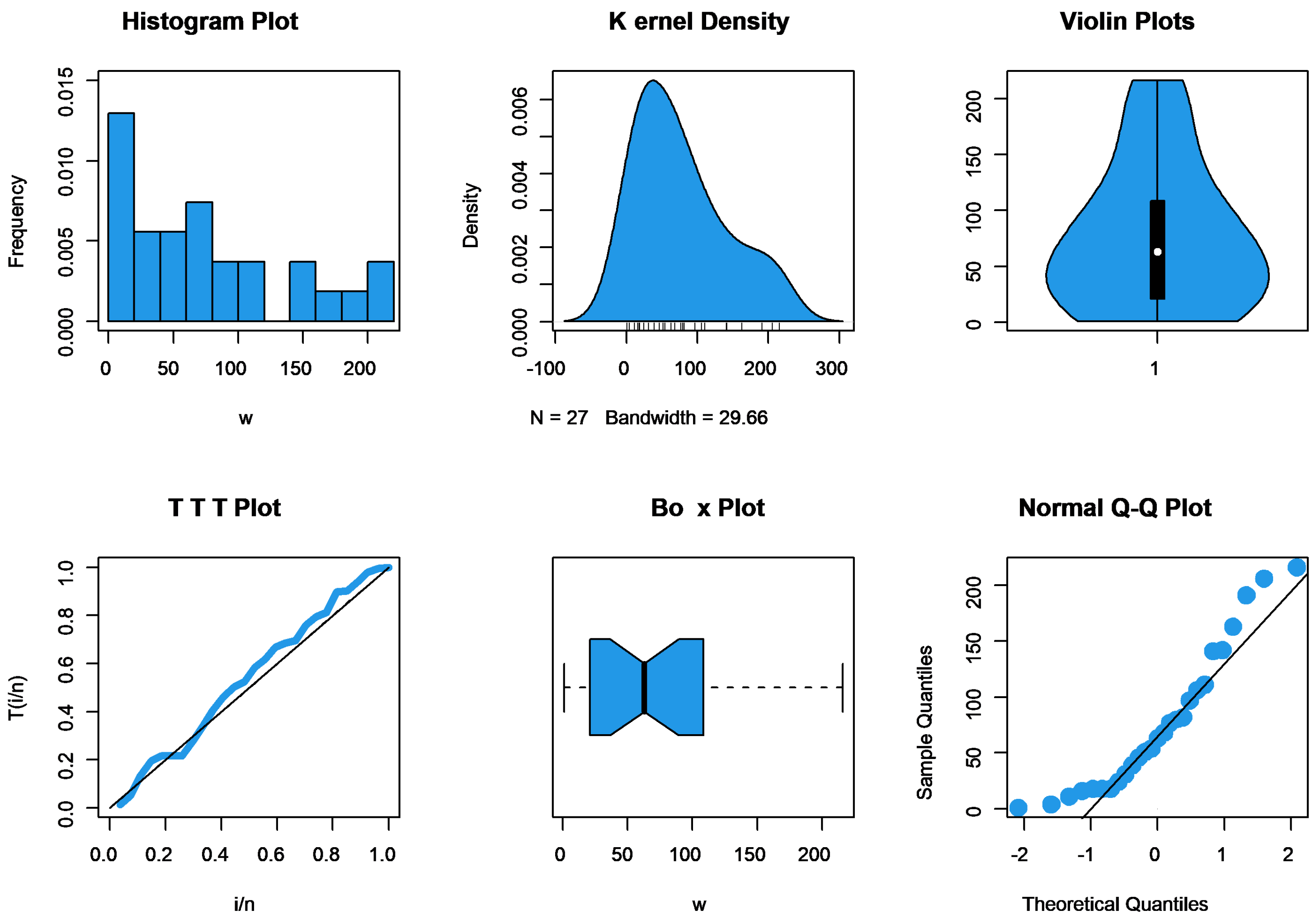
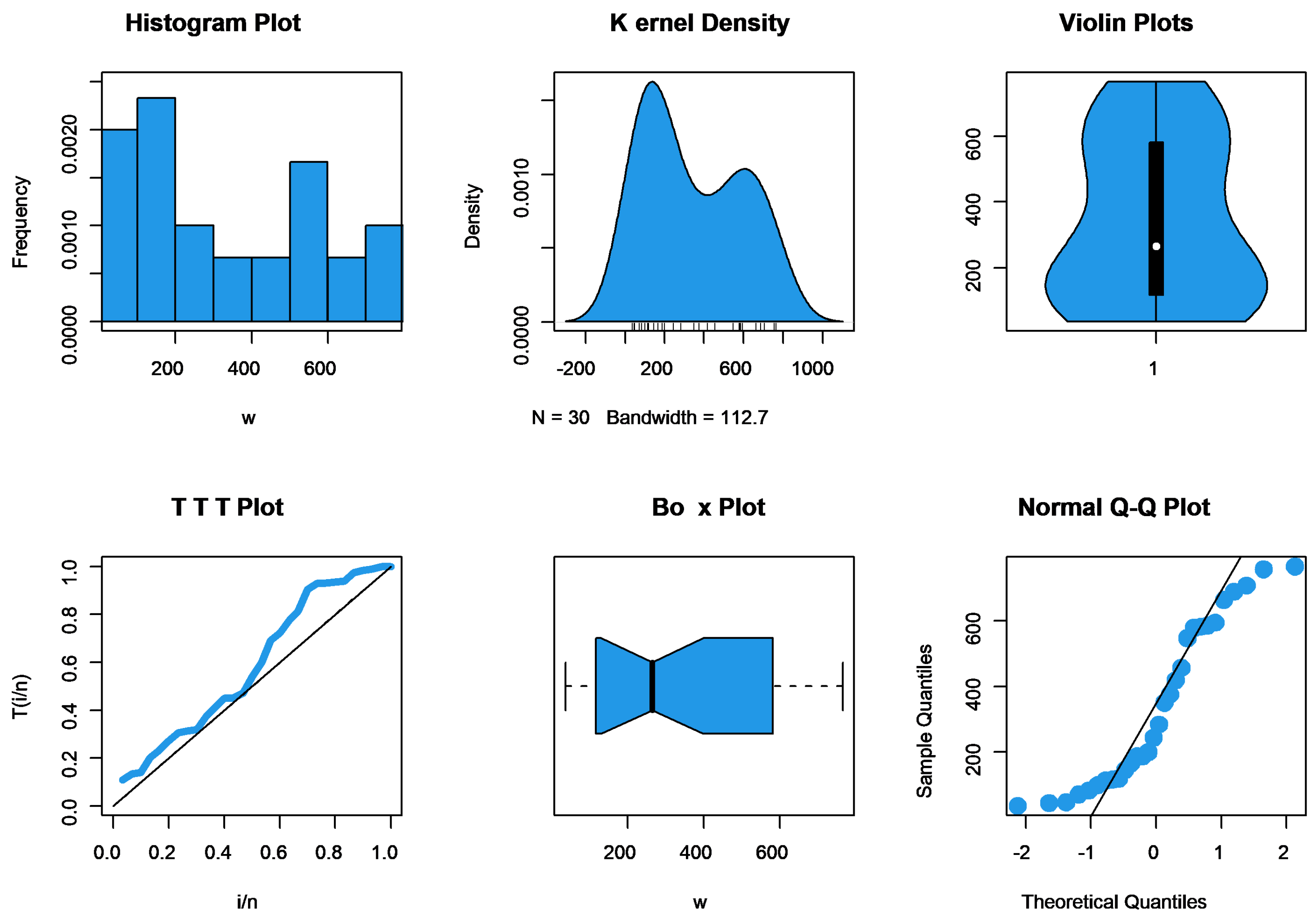
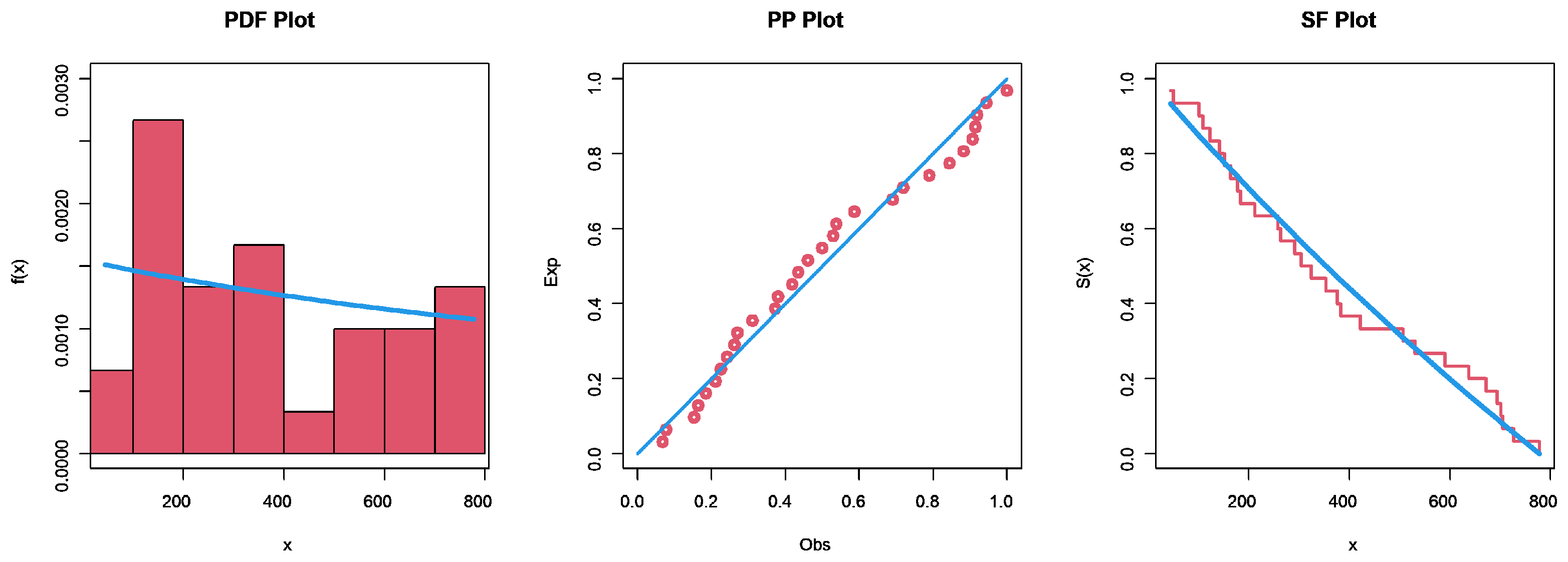
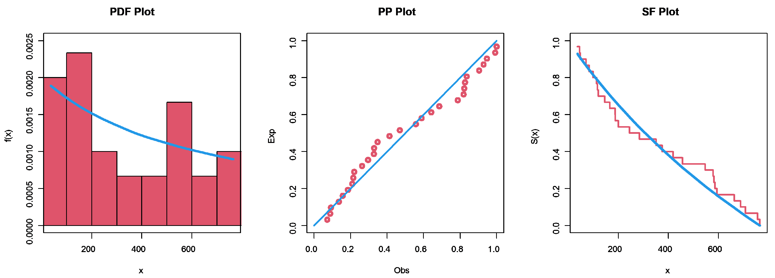
6. Application to Jute Fiber

To clarify the significance of the theoretical discoveries discussed in the preceding sections, this section will detail an application with jute fiber. The analysis of the real-world data set in this section lends validity to the suggested point and interval estimates for the SSR parameter R. In this application, we take into account data of the breaking strengths of jute fiber at two different gauge lengths, which are provided by Xia et al. [36]. Saracoglu et al. [18] also provided an illustration of these data for evaluation. The sets of data are: Breaking strength of jute fiber of gauge length 10 mm (strength—X), 693.73, 704.66, 323.83, 778.17, 123.06, 637.66, 383.43, 151.48, 108.94, 50.16, 671.49, 183.16, 257.44, 727.23, 291.27, 101.15, 376.42, 163.40, 141.38, 700.74, 262.90, 353.24, 422.11, 43.93, 590.48, 212.13, 303.90, 506.60, 530.55, 177.25. Breaking strength of jute fiber of gauge length 20 mm (stress—Y), 71.46, 419.02, 284.64, 585.57, 456.60, 113.85, 187.85, 688.16, 662.66, 45.58, 578.62, 756.70, 594.29, 166.49, 99.72, 707.36, 765.14, 187.13, 145.96, 350.70, 547.44, 116.99, 375.81, 581.60, 119.86, 48.01, 200.16, 36.75, 244.53, 83.55. Figure 1 and Figure 2 illustrate the nonparametric kernel density (KD) estimation approach used to examine the initial density shape. It is noticed that for data sets I and II, respectively, the initial density shape is asymmetric and unimodal (bimodal) functions. Figure 1 and Figure 2’s quantile–quantile (Q-Q) and TTT plots are used to test the normality condition and hazard rate shapes. The box and violin plots in Figure 1 and Figure 2 reveal the extremes, and it is demonstrated that several extreme observations were supported. For the purposes of the goodness of fit test, the Kolmogorov–Smirnov (K-S) separation between the fitted distribution function and the empirical distribution function was determined. This value is $0.095255$ for set I and has a p-value of $0.9244$, whereas it is $0.12041$ for set II and has a p-value of $0.7325$. As a result, the p-value for K-S was highest for sets I and II. It is safe to say that the UTNBD better fits the two real data sets. The empirical plots in Figure 3 and Figure 4 show how the UTNBD clearly fits the data.

By using the censoring scheme $S=(2,0,2,0,1,0,3,0,2,0,0,1,0,1,0,0,0,0),$ we generate a progressively type-II censored (PTIIC) sample of size $m_1=18,$ from set I with $n_1=30$. The obtained PT2C sample is 43.93, 50.16, 101.15, 108.94, 141.38, 151.48, 163.4, 177.25, 183.16, 212.13, 257.44, 353.24, 376.42, 383.43, 422.11, 590.48, 700.74, and 727.23. For set II, suppose that the censoring scheme is given by $T=(1,1,2,1,1,2,1,2,1,1,2,0,0,0,0)$, then a PTIIC sample of size $m_2=15$ out of $n_2=30$ items of data is obtained as 36.75, 45.58, 48.01, 71.46, 83.55, 145.96, 166.49, 187.13, 187.85, 200.16, 578.62, 581.6, 585.57, 662.66, and 756.7.

The MLE of R and its associated ACI are calculated under the PTIIC implementation on the strength variable X and stress variable Y as follows: ${\widehat{R}}_{ML}=0.477182$ and $(0.37526,0.58538)$ with average interval width $0.21012$. Additionally, the BP and BT are computed as $0.473537$ and $0.445765$ by including the iterative techniques discussed in Section 3, and their associated ACIs are computed as $(0.346753,0.552464)$ and $(0.357472,0.519763)$, with AWs of $0.205711$ and $0.162291$, respectively. In order to delve into the uniqueness property, we have generated log-likelihood profiles and observed that all estimators exhibit unimodal shapes. Please consult Figure 5, which serves as an illustrative schema for further details for the model estimators.

It is now necessary to describe the prior distributions for the parameters $\alpha ,$${\lambda }_1$ and ${\lambda }_2$ in order to obtain the Bayesian estimate of R. We make the assumption that the noninformative gamma priors for $\alpha ,$${\lambda }_1$ and ${\lambda }_2$, i.e., when the hyperparameters are $a_i=0.0001$ and $b_i=0.0001,$$i=1,2,3$ are applicable as we lack prior knowledge. The initial values for the parameters $\alpha ,$${\lambda }_1$, ${\lambda }_2$ and $\theta$ were taken to be their MLEs and ${\theta }_0=765.14$ in order to run the MCMC procedure outlined in Section 4. Furthermore, 12,000 MCMC samples were produced. We remove the first 2000 samples as ’burn-in’ to eliminate the impact of the initial values. As a result, the Bayesian estimate of R and its corresponding CRI is calculated as ${\widehat{R}}_{MC}=0.46876$ and $(0.399967,0.561374)$ with average interval width $0.161407$. Figure 6 shows R’s 12,000 chain values. The R kernel density estimation and histogram are displayed in Figure 7.

7. Summary Findings

In this article, we explored the estimation of the stress–strength reliability (SSR) parameter $R=P(Y<X)$ within the context of progressive type-II interval censoring (PTIIC) for two independent random variables: strength X and stress Y. Both X and Y followed a uniform truncated negative binomial distribution with identical shape and scale parameters. We employed various estimation methods in this study. First, we derived maximum likelihood estimators (MLEs) and asymptotic confidence intervals for the SSR parameter R using the observed Fisher information matrix. Additionally, we proposed two parametric bootstrap methods for constructing confidence intervals, with the finding that one of them, referred to as BT, remained highly effective even with small effective sample sizes. Furthermore, we explored the Bayesian estimation of R under the squared error loss function, utilizing an independent gamma prior. Because Bayesian estimators involved ratios of integrals that could not be analytically solved, we employed importance sampling techniques coupled with the Metropolis–Hastings algorithm to compute Bayes estimates along with credible intervals. To assess the performance of these estimation methods, we conducted a comprehensive simulation study that considered various sample sizes $(n_i,m_i),i=1,2$, censoring schemes (I, II, and III), and combinations of unknown parameters $\left(\alpha ,{\lambda }_1,{\lambda }_2\right)$. This empirical comparison was necessary because a theoretical comparison was not feasible. The simulation results led us to two key conclusions. First, in cases where PTIIC data from multiple uniform truncated negative binomial distributions were available, the Bayesian technique was effectively employed to estimate the SSR parameter R and generate approximate confidence intervals. Second, the importance sampling approach consistently outperformed the maximum likelihood and bootstrap methods, demonstrating commendable performance. Overall, this study underscored the utility of the uniform truncated negative binomial distribution in accurately modeling real-world data, particularly in medical and engineering applications.

References

1. Kotz, S.; Lumelskii, Y.; Pensky, M. The Stress-Strength Model and Its Generalization: Theory and Applications; World Scientific: Singapore, 2003. [Google Scholar]
2. Church, J.D.; Harris, B. The estimation of the reliability from stress–strength relationships. Technometrics 1970, 12, 49–54. [Google Scholar] [CrossRef]
3. Surles, J.G.; Padgett, W.J. Inference for P(Y < X) in the Burr Type X model. J. Appl. Stat. Sci. 1998, 7, 225–238. [Google Scholar]
4. Surles, J.G.; Padgett, W.J. Inference for reliability and stress–strength for a scaled Burr-Type X distribution. Lifetime Data Anal. 2001, 7, 187–200. [Google Scholar] [CrossRef]
5. Kundu, D.; Gupta, R.D. Estimation of P(Y < X) for generalized exponential distribution. Metrika 2005, 61, 291–308. [Google Scholar]
6. Raqab, M.Z.; Kundu, D. Comparison of different estimators of P(Y < X) for a scaled Burr type X distribution. Commun. Stat. Simul. Comput. 2005, 34, 465–483. [Google Scholar]
7. Kundu, D.; Gupta, R.D. Estimation of P(Y < X) for Weibull Distribution, IEEE Trans. Reliab. 2006, 55, 270–280. [Google Scholar]
8. Nadar, M.; Kizilaslan, F.; Papadopoulos, A. Classical and Bayesian estimation of P(Y < X) for Kumaraswamy distribution. Stat. Comput. Simul. 2014, 84, 1505–1529. [Google Scholar]
9. Sharma, V.K.; Singh, S.K.; Singh, U.; Agiwal, V. The inverse Lindley distribution: A stress-strength reliability model with application to head and neck cancer data. J. Ind. Prod. 2015, 32, 162–173. [Google Scholar] [CrossRef]
10. Ahmed, A.; Batah, F. On the estimation of stress-strength model reliability parameter of power rayleigh distribution. Iraqi J. Sci. 2023, 64, 809–822. [Google Scholar] [CrossRef]
11. Baklizi, A. Estimation of P(Y < X) using record values in the one and two parameter exponential distributions. Valiollahi 2008, 37, 692–698. [Google Scholar]
12. Nadar, M.; Kizilaslan, F. Classical and Bayesian estimation of P[Y < X] using upper record values from Kumaraswamy distribution. Stat. Pap. 2014, 55, 751–783. [Google Scholar]
13. Mahmoud, A.W.M.; EL-Sagheer, R.M.; Soliman, A.A.; Abd Ellah, A.H. Bayesian estimation of P[Y < X] based on record values from the Lomax distribution and MCMC technique. J. Mod. Appl. Stat. 2016, 15, 488–510. [Google Scholar]
14. Hasan, A.S.; Abd-Allah, M.; Nagy, H.F. Estimation of P(Y < X) using record values from the generalized inverted exponential distribution. Pak. J. Stat. Oper. Res. 2018, XIV, 645–660. [Google Scholar]
15. Balakrishnan, N.; Sandhu, R.A. A simple simulation algorithm for generating progressive type-II censored samples. Am. Assoc. 1995, 49, 229–230. [Google Scholar]
16. Yu, Y.; Wang, L.; Dey, S.; Liu, J. Estimation of stress-strength reliability from unit-Burr III distribution under records data. Math. Biosci. Eng. 2023, 20, 12360–12379. [Google Scholar] [CrossRef]
17. Koul, S.; Chaturvedi, A. Estimation and testing procedures for the reliability functions of one parameter generalized exponential distribution. Thail. Stat. 2023, 21, 268–290. [Google Scholar]
18. Saracoglu, B.; Kinaci, I.; Kundu, D. On estimation of R = P(Y < X) for exponential distribution under progressive type II censoring. Stat. Comput. Simul. 2012, 82, 729–744. [Google Scholar]
19. Valiollahi, R.; Asgharzadeh, A.; Raqab, M.Z. Estimation of P(Y < X) for Weibull distribution under progressive type II censoring. Commun. Stat. Theory Methods 2013, 42, 4476–4498. [Google Scholar]
20. Kumar, K.; Krishna, H.; Garg, R. Estimation of P(Y < X) in Lindley distribution using progressively first failure censoring. Int. J. Syst. Assur. Eng. Manag. 2015, 6, 330–341. [Google Scholar]
21. Krishna, H.; Dube, M.; Garg, R. Estimation of P(Y < X) for progressively first failure censored generalized inverted exponential distribution. Stat. Comput. Simul. 2017, 87, 2274–2289. [Google Scholar]
22. EL-Sagheer, R.M.; Mansour, M.M.M. The efficacy measurement of treatment methods: An application to stress-strength model. Appl. Math. Inf. Sci. 2020, 14, 487–492. [Google Scholar]
23. Kamel, B.I.; Abo Youssef, S.E.; Sief, M.G. The Uniform truncated negative binomial distribution and its properties. J. Math. Stat. 2016, 12, 290–301. [Google Scholar] [CrossRef]
24. EL-Sagheer, R.M. Estimation of parameters of Weibull-Gamma distribution based on progressively censored data. Stat. Pap. 2018, 59, 725–757. [Google Scholar] [CrossRef]
25. Casella, G.; Berger, R.L. Statistical Inference, 2nd ed.; Duxbury Press: Pacific Grove, CA, USA, 2002. [Google Scholar]
26. Xu, J.; Long, J.S. Using the delta method to construct confidence intervals for predicted probabilities, rates, and discrete changes. Stata J. 2005, 5, 537–559. [Google Scholar] [CrossRef]
27. Efron, B. Bootstrap methods: Another look at the jackknife. Ann. Stat. 1979, 27, 1–26. [Google Scholar] [CrossRef]
28. Davison, A.C.; Hinkley, D.V. Bootstrap Methods and Their Application; Cambridge University Press: Cambridge, UK, 1997. [Google Scholar]
29. DiCiccio, T.J.; Efron, B. Bootstrap confidence intervals. Stat. Sci. 1996, 11, 189–212. [Google Scholar] [CrossRef]
30. Efron, B.; Tibshirani, R. An Introduction to the Bootstrap; Chapman & Hall: New York, NY, USA, 1994. [Google Scholar]
31. Arnold, B.C.; Press, S.J. Bayesian inference for Pareto populations. Econometrics 1983, 21, 287–306. [Google Scholar] [CrossRef]
32. Upadhyay, S.K.; Vasistha, N.; Smith, A.F.M. Bayes inference in life testing and reliability via Markov chain Monte Carlo simulation. Sankhya A 2001, 63, 15–40. [Google Scholar]
33. Kundu, D.; Howlader, H. Bayesian inference and prediction of the inverse Weibull distribution for Type-II censored data. Comput. Stat. Data Anal. 2010, 54, 1547–1558. [Google Scholar] [CrossRef]
34. Chen, M.-H.; Shao, Q.-M. Monte Carlo estimation of Bayesian credible and HPD intervals. J. Comput. Graph. 1999, 8, 69–92. [Google Scholar]
35. Hastings, W.K. Monte Carlo sampling methods using Markov chains and their applications. Biometrika 1970, 57, 97–109. [Google Scholar] [CrossRef]
36. Xia, Z.P.; Yu, J.Y.; Cheng, L.D.; Liu, L.F.; Wang, W.M. Study on the breaking strength of jute fibres using modified Weibull distribution. Compos. Part Appl. Sci. Manuf. 2009, 40, 54–59. [Google Scholar] [CrossRef]
Figure 1. The KD, box, TTT, QQ, and violin plots for data set I.
Axioms 12 00949 g001
Figure 2. The KD, box, TTT, QQ, and violin plots for set II.
Axioms 12 00949 g002
Figure 3. Empirical, PP, and SF plots for set I.
Axioms 12 00949 g003
Figure 4. Empirical, PP, and SF plots for set II.
Axioms 12 00949 g004
Figure 5. The log-likelihood profiles.
Axioms 12 00949 g005
Figure 6. MCMC trace plot of R.
Axioms 12 00949 g006
Figure 7. Histogram of R.
Axioms 12 00949 g007