Article

Lattice Boltzmann Model for a Class of Time Fractional Partial Differential Equation

College of Science, Shenyang University of Technology, Shenyang 110870, China
*
Author to whom correspondence should be addressed.
Axioms 2023, 12(10), 959; https://doi.org/10.3390/axioms12100959
Submission received: 1 September 2023 / Revised: 3 October 2023 / Accepted: 9 October 2023 / Published: 11 October 2023

Abstract

:
This paper is concerned with the lattice Boltzmann (LB) method for a class of time fractional partial differential equations (FPDEs) in the Caputo sense. By utilizing the properties of the Caputo derivative and discretization in time, FPDEs can be approximately transformed into standard partial differential equations with integer orders. Through incorporating an auxiliary distribution function into the evolution equation, which assists in recovering the macroscopic quantity u, the LB model with spatial second-order accuracy is constructed. The numerical experiments verify that the numerical results are in good agreement with analytical solutions and that the accuracy of the present model is better than the previous solutions.

1. Introduction

Fractional partial differential equations (FPDEs) have received an increasing attention in recent years and have been widely applied in fields such as viscoelastic materials, chemistry, engineering, biology, physics, economics, and so on [1,2,3,4,5,6,7,8,9]. Compared with the classical integer order model, the main advantage of the fractional order model lies in its capacity to effectively describe materials and processes with genetic and memory properties. Therefore, it is both theoretical and practical to study the properties and numerical methods of FPDEs. In this paper, we consider the following time FPDE in the Caputo sense
0 C D t α u ( x , t ) B Δ u ( x , t ) = F ( x , t , u ) , ( x , t ) Ω × ( 0 , T ] ,
with the initial conditions
u ( x , 0 ) = u 0 ( x ) , x Ω ,
and boundary conditions
u ( x , t ) = φ ( x , t ) , x 𝜕 Ω , 0 < t T ,
where 0 < α < 1 is the fractional order, B is a constant, u ( x , t ) is a scalar function of position x and time t, Δ is the Laplace operator, φ ( x , t ) is the boundary condition and φ ( x , 0 ) = 0 , and Ω is a continuous domain in space with suitable boundary conditions prescribed on its boundary 𝜕 Ω . The Caputo fractional derivative 0 C D t α u ( x , t ) can be written as
0 C D t α u ( x , t ) = 1 Γ ( 1 α ) 0 t 𝜕 u ( x , ξ ) 𝜕 ξ d ξ ( t ξ ) α , 0 < α < 1 , 𝜕 u ( x , t ) 𝜕 t , α = 1 ,
where Γ ( · ) is the Gamma function. It is worth noting that the nonlinear term F ( x , t , u ) of Equation (1) can be taken of different forms, which corresponds to different equations. Some special cases of Equation (1) have been seen as follows:
(i)
When F = f ( x , t ) , Equation (1) reduces to a classical time fractional sub-diffusion equation
0 C D t α u ( x , t ) B Δ u ( x , t ) = f ( x , t ) ,
which is used to describe anomalous diffusion behaviors with a very wide range of applications in mechanics and chemistry [10].
(ii)
When F = a u ( x , t ) ( 1 u b ( x , t ) ) , Equation (1) reduces to a classical time fractional Fisher’s equation
0 C D t α u ( x , t ) B Δ u ( x , t ) = a u ( x , t ) ( 1 u b ( x , t ) ) ,
which was originally proposed by Fisher [11] in 1937 as a model for the spatial and temporal propagation of a virile gene in an infinite medium, where a and b are real parameters.
(iii)
When F = c ( 1 u ) ( u d ) , Equation (1) reduces to a classical time fractional Huxley equation
0 C D t α u ( x , t ) B Δ u ( x , t ) = c ( 1 u ( x , t ) ) ( u ( x , t ) d ) ,
which is a nonlinear reaction-diffusion model describing neural dynamics and has important applications in various fields, such as biology, fluid dynamics [12,13], etc.
The analytical solutions of FPDEs are usually studied using the Fourier transform method or the Green function method [1,14,15]. However, for most FPDEs it is difficult to obtain analytical solutions due to the limitations of the initial boundary problem and the complexity of the fractional derivative. For these reasons, some numerical methods have been proposed, including the finite difference method [16,17], the meshless method [18,19], the spectral method [20], the finite element method [21,22], the natural decomposition method [23], and so on [24,25]. Since most numerical methods in the literature are either too complicated to implement or have low computational efficiency, it is desirable to have alternative ways to solve the FPDEs.
In recent decades, the lattice Boltzmann (LB) method originated from kinetic theory has been used with great success in hydrodynamics [26,27]. Compared with conventional numerical methods, it involves only simple arithmetic calculations, high parallelism, and efficiently handles complicated boundary conditions. In addition, the LB method has been developed to simulate linear and nonlinear partial differential equations, and interested readers may wish to consult these documents [28,29,30,31,32,33,34,35,36,37]. Compared with the extensive LB method studies on the classical partial differential equations, there are limited studies on FPDEs. Du et al. [38] constructed a general LB model for time fractional sub-diffusion equation in the Caputo sense by using a composite integration rule and linear interpolation. Zhang et al. [39] presented a LB model for the fractional sub-diffusion equation in a Riemann–Liouville sense and an intermediate quantity which is approximated using the definition of Grünwald–Letnikov fractional derivative was introduced into the model. Recently, liang and zhang et al. [40] proposed a new LB method for the fractional Cahn–Hilliard equation. The idea of the model is to first approximate the fractional derivative based on the Caputo sense using a composite integration rule and linear interpolation, then the modified equilibrium distribution function and proper source term are incorporated into the LB method in order to recover the targeting equation. In this paper, we construct an LB model for FPDEs in the Caputo sense by adding a distribution function which is completely independent from the distribution function of the source term in order to auxiliary recover the macroscopic term u ( x , t ) . The model presented in this paper has a simple form and can be easily implemented in numerical simulations.
This paper is organized as follows. In Section 2, the LB model for a class of FPDEs is described. The proposed model is verified by several numerical examples in Section 3. Finally, conclusions are summarized in Section 4.

2. Lattice Boltzmann Method for FPDEs

2.1. Governing Equation

Since it is difficult to construct LB methods for FPDEs directly, it is necessary to transform Equation (1) into an appropriate form using the composite integration rule and the piecewise linear interpolation. Let t n = n Δ t , where Δ t = T / N t is the time step, and let n = 0 , 1 , , N t be mesh points, where N t is a positive integer. At t = t n , the derivative term 0 C D t α u ( x , t ) can be approximated by [38]
0 C D t α u ( x , t n ) = 1 Γ ( 1 α ) k = 1 n 1 t k 1 t k 𝜕 u ( x , ξ ) 𝜕 ξ d ξ ( t n ξ ) α + 1 Γ ( 1 α ) t n 1 t n 𝜕 u ( x , ξ ) 𝜕 ξ d ξ ( t n ξ ) α Δ t α Γ ( 2 α ) k = 1 n 1 ( n k + 1 ) 1 α ( n k ) 1 α u x , t k u x , t k 1 + Δ t 1 α Γ ( 2 α ) 𝜕 u ( x , t n ) 𝜕 t .
Substituting Equation (8) into Equation (1), we have
γ 𝜕 u ( x , t n ) 𝜕 t B Δ u ( x , t n ) = H ( t n , u ) + F ( x , t n , u ) ,
where γ = Δ t 1 α Γ ( 2 α ) and H ( t n , u ) denotes
H ( t n , u ) = γ Δ t k = 0 n 1 ( n k + 1 ) 1 α ( n k ) 1 α u x , t k u x , t k 1 .

2.2. Lattice Boltzmann Model

The lattice Boltzmann model applied in this paper is the Bhatnagar–Gross–Krook model with DnQb lattice (b is the number of discrete directions in nD space) [41]. The evolution equation for Equation (9) is written as
f α ( x + e α Δ t , t + Δ t ) f α ( x , t ) = 1 τ [ f α ( x , t ) f α e q ( x , t ) ] + Δ t H α ( t , u ) + Δ t F α ( x , t , u ) ,
where f α ( x , t ) is the local particle distribution function with velocity e α , f α e q ( x , t ) is the equilibrium distribution function, and Δ x and Δ t represent the discrete steps of space and time, respectively. τ is the dimensionless relaxation time. H α ( t , u ) is the distribution function which is used to auxiliary recover the macroscopic term u ( x , t ) , F α ( x , t , u ) is the distribution function of the source term. And the macroscopic expression for u ( x , t ) can be written as
γ u ( x , t ) = α f α ( x , t ) + τ Δ t 2 τ 1 H α ( t , u ) .
By applying the Taylor expansion to Equation (11), we have
Δ t ( 𝜕 𝜕 t + e α 𝜕 𝜕 x ) f α + Δ t 2 2 ( 𝜕 𝜕 t + e α 𝜕 𝜕 x ) 2 f α + O ( ε 3 ) = 1 τ ( f α f α e q ) + Δ t H α ( t , u ) + Δ t F α ( x , t , u ) .
The multi-scale Chapman–Enskog expansion up to first-order in space and second-order in time is applied, we have
𝜕 𝜕 x = ε 𝜕 𝜕 x 1 + O ( ε 2 ) ,
𝜕 𝜕 t = ε 𝜕 𝜕 t 1 + ε 2 𝜕 𝜕 t 2 + O ( ε 3 ) ,
where ε is a small expansion parameter. The distribution function and the auxiliary function are then expanded
f α = f α ( 0 ) + ε f α ( 1 ) + ε 2 f α ( 2 ) + ,
F α = ε 2 F α ( 2 ) + ,
H α = ε H α ( 1 ) + ,
H = ε H ( 1 ) + .
Substituting Equations (14)–(19) into Equation (13), we obtain an equation of order ε 0
f α ( 0 ) = f α e q ,
the equation of order ε 1 is
O ( ε 1 ) : ( 𝜕 𝜕 t 1 + e α 𝜕 𝜕 x 1 ) f α ( 0 ) = 1 τ Δ t f α ( 1 ) + H α ( 1 ) ,
and the equation of order ε 2 is
O ( ε 2 ) : 𝜕 𝜕 t 2 f α ( 0 ) + ( 𝜕 𝜕 t 1 + e α 𝜕 𝜕 x 1 ) f α ( 1 ) + Δ t 2 ( 𝜕 𝜕 t 1 + e α 𝜕 𝜕 x 1 ) 2 f α ( 0 ) = 1 τ Δ t f α ( 2 ) + F α ( 2 ) .
In order to recover the macroscopic Equation (9) correctly, some constraints on the higher moments of the local equilibrium distribution function are imposed as
f α e q = γ u ,
α e α f α e q = 0 ,
α e α e α f α e q = λ u I ,
where I is the unit matrix and λ is a real parameter to be determined by the coefficient B and relaxation time τ . The auxiliary distribution function and the distribution function of source term should satisfy
H α = ε H α ( 1 ) = ( 1 1 2 τ ) H ,
e α H α = ε e α H α ( 1 ) = 0 ,
F α = ε 2 F α ( 2 ) = F .
According to Equations (12), (16), (19), (23), and (26), we have
f α ( 1 ) = Δ t 2 H ( 1 ) ,
f α ( k ) = 0 , k > 1 .
According to Equations (21), (24), (25), and (27), we have
e α f α ( 1 ) = ( τ Δ t ) e α 𝜕 𝜕 t 1 + e α 𝜕 𝜕 x 1 f α ( 0 ) H α ( 1 ) = τ Δ t 𝜕 𝜕 t 1 e α f α ( 0 ) + 𝜕 𝜕 x 1 e α e α f α ( 0 ) e α H α ( 1 ) = τ Δ t 𝜕 𝜕 x 1 e α e α f α ( 0 ) .
Summing Equation (21) over α , and using Equations (19), (23), (24), and (29) we obtain
O ε 1 : 𝜕 ( γ u ) 𝜕 t 1 = H ( 1 ) .
Summing Equation (22) over α , and using Equations (19), (21), (23), (25), and (27)–(31) we obtain
O ( ε 2 ) : 𝜕 ( γ u ) 𝜕 t 2 + ( 1 1 2 τ ) ( τ Δ t ) 𝜕 𝜕 x 1 · ( 𝜕 𝜕 x 1 λ u ) = 1 τ Δ t f α ( 2 ) + 1 ε 2 F .
Finally, the macroscopic equation with the second-order accuracy of truncation error can be obtained by taking Equation (32) × ε + Equation (33) × ε 2 :
γ 𝜕 u 𝜕 t Δ · Δ t τ 1 2 λ u + O ( ε 3 ) = F ( x , t , u ) + H ( t , u ) ,
where λ = B Δ t τ 1 2 .
Different lattice discrete velocity models are chosen in this paper, for D1Q3 model, e 0 , e 1 , e 2 = { 0 , c , c } ; for D1Q5 model, e 0 , e 1 , e 2 , e 3 , e 4 = { 0 , c , c , 2 c , 2 c } ; and for D2Q9 model, e j , j = 0 , , 8 = { ( 0 , 0 ) , ( ± c , 0 ) , ( 0 , ± c ) , ( ± c , ± c ) } . Based on the above velocity models, the equilibrium distribution function f α e q , the auxiliary distribution function H α and the distribution function of source term F α can be obtained from Equations (23)–(29), respectively, as follows
  • D1Q3 lattice
    f α e q = B u 2 Δ t ( τ 1 2 ) c 2 , α = 1 , 2 , γ u B u Δ t ( τ 1 2 ) c 2 , α = 0 , H α = 1 3 ( 1 1 2 τ ) H , α = 0.1 , 2 , F α = 1 6 F , α = 1 , 2 , 2 3 F , α = 0 .
  • D1Q5 lattice
    f α e q = B u 6 Δ t ( τ 1 2 ) c 2 , α = 1 , 2 , B u 12 Δ t ( τ 1 2 ) c 2 , α = 3 , 4 , γ u B u 2 Δ t ( τ 1 2 ) c 2 , α = 0 , H α = 1 5 ( 1 1 2 τ ) H , α = 0 , , 4 , F α = 1 6 F , α = 1 , 2 , 1 12 F , α = 3 , 4 , 1 2 F , α = 0 .
  • D2Q9 lattice
    f α e q = B u 3 Δ t ( τ 1 2 ) c 2 , α = 1 , , 4 , B u 12 Δ t ( τ 1 2 ) c 2 , α = 5 , , 8 , γ u 5 B 3 c 2 u , α = 0 , H α = 1 9 ( 1 1 2 τ ) H , α = 0 , , 8 , F α = 1 9 F , α = 1 , , 4 , 1 36 F , α = 5 , , 8 , 4 9 F , α = 0 .

3. Numerical Simulations

To show the effectiveness of the models proposed above, we simulate several numerical experiments with appropriate initial and boundary conditions at different parameter choices. The distribution functions f α ( x , t ) are initialized by setting to be f α e q ( x , t ) . The non-equilibrium extrapolation scheme proposed by Guo et al. [42] is employed to deal with the boundary conditions. In addition, to test the precision of the present models, the maximum absolute error ( MAE ) and the global relative error ( GRE ) are defined as follows:
MAE = max i | u ( x i , t ) u * ( x i , t ) | ,
GRE = i u x i , t u * x i , t i u * x i , t ,
where u ( x i , t ) and u * ( x i , t ) are the numerical solution and exact solution, respectively.
Example 1.
Consider the following one dimensional sub-diffusion Equation [38]
0 C D t α u = B 𝜕 2 u 𝜕 x 2 + g ( x , t ) , x [ 0 , L ] , 0 < t T ,
u ( x , 0 ) = 0 , x [ 0 , L ] ,
u ( 0 , t ) = t 2 , u ( L , t ) = t 2 e , 0 < t T ,
where g ( x , t ) = [ 2 Γ ( 3 α ) t 2 α B t 2 ] e x ; the exact solution can be given by u ( x , t ) = t 2 e x .
In the computation, we take L = 1.0 , B = 0.0001 , the time step Δ t = 0.0001 , the space step Δ x = 1 / 128 ( M = 128 ) , and τ = 1 for α = 0.2 , 0.3 , τ = 1.01 for α = 0.5 , and τ = 1.1 for α = 0.8 , respectively. Figure 1 shows the numerical solutions and exact solutions at different time, and it can be seen that they are in good agreement. Table 1 shows the comparison results of the GREs and MAEs between the proposed method and the LB method of DU et al. [38] for different lattice sizes and α . As shown in this table, our method has higher accuracy and the errors decrease as the lattice size increases for different α . Table 2 shows the errors when α are taken to smaller values at t = 1.0 . Figure 2 shows the log–log plots of the GREs and MAEs versus space step at t = 1 with different α . From Figure 2, it can be seen that the slopes of the fitting lines for different results are about 2.0, indicating that the model in this paper has the second-order accuracy in space, which is consistent with the theoretical accuracy.
In addition, we take B = 0.001 , α = 0.9 , τ = 1.34 , Δ t = 0.0001 , and Δ x = 1 / 128 . Table 3 presents the comparison results of the GREs and MAEs for the proposed method and the LB method of Zhang et al. [39]. It can be seen that our method has significantly higher accuracy.
Example 2.
Consider the following two dimensional sub-diffusion problem,
0 C D t α u = B 𝜕 2 u 𝜕 x 2 + 𝜕 2 u 𝜕 y 2 + g ( x , y , t ) , ( x , y ) Ω , 0 < t T .
(a)
In this case, the source term of sub-diffusion equation in [38] is
g ( x , y , t ) = 2 Γ ( 3 α ) t 2 α + 8 B π 2 t 2 sin ( 2 π x ) sin ( 2 π y ) ,
the initial conditions are
u ( x , y , 0 ) = 0 , ( x , y ) Ω ,
the boundary conditions are
u ( x , y , t ) 𝜕 Ω = 0 , 0 < t T ,
and the exact solution is
u ( x , y , t ) = t 2 sin ( 2 π x ) sin ( 2 π y ) .
In the computation, we take Ω = [ 0 , 1 ] × [ 0 , 1 ] , B = 0.0001 , Δ x = Δ y = 1 / 64 ( M = N = 64 ) , and Δ t = 0.001 . Figure 3 shows the numerical solutions and exact solutions at different α along x at y = 0.25 . It can be found that the numerical and exact solutions are in good agreement. Figure 4 shows the time evolution of the numerical solutions for different α at t = 1 , and Figure 5 plots the contour graphs of the numerical solutions and errors for α = 0.2 , 0.3 , 0.5 , 0.8 at different times; errors in this figure are denoted by | u ( x i , t ) u * ( x i , t ) | . Table 4 shows the comparison results of the MAEs between the present method and the LB method of DU et al. [38] at different lattice sizes and α . From Table 4 it can be seen that our method has higher accuracy and the errors decrease as the lattice size increases. Table 5 gives the MAEs and GREs with different time and α .
(b)
Consider the two dimensional sub-diffusion equation in [39], the source term of this problem is
g ( x , y , t ) = 2 Γ ( 3 α ) t 2 α 2 B t 2 e x + y ,
the initial conditions are
u ( x , y , 0 ) = 0 , ( x , y ) Ω ,
the boundary conditions are
u ( 0 , y , t ) = t 2 e y ,
u ( 1 , y , t ) = t 2 e 1 + y ,
u ( x , 0 , t ) = t 2 e x ,
u ( x , 1 , t ) = t 2 e 1 + x ,
and the exact solution is
u ( x , y , t ) = t 2 e x + y .
In the computation, we take Ω = [ 0 , 1 ] × [ 0 , 1 ] , B = 0.001 , α is fixed to be 0.9, Δ x = Δ y = 1 / 170 ( M = N = 170 ) , Δ t = 0.001 . Table 6 lists the comparison results solved by the present method with the results by method of Zhang et al. [39]. It can be found that for two dimensional numerical experiment, our method is still more accurate.
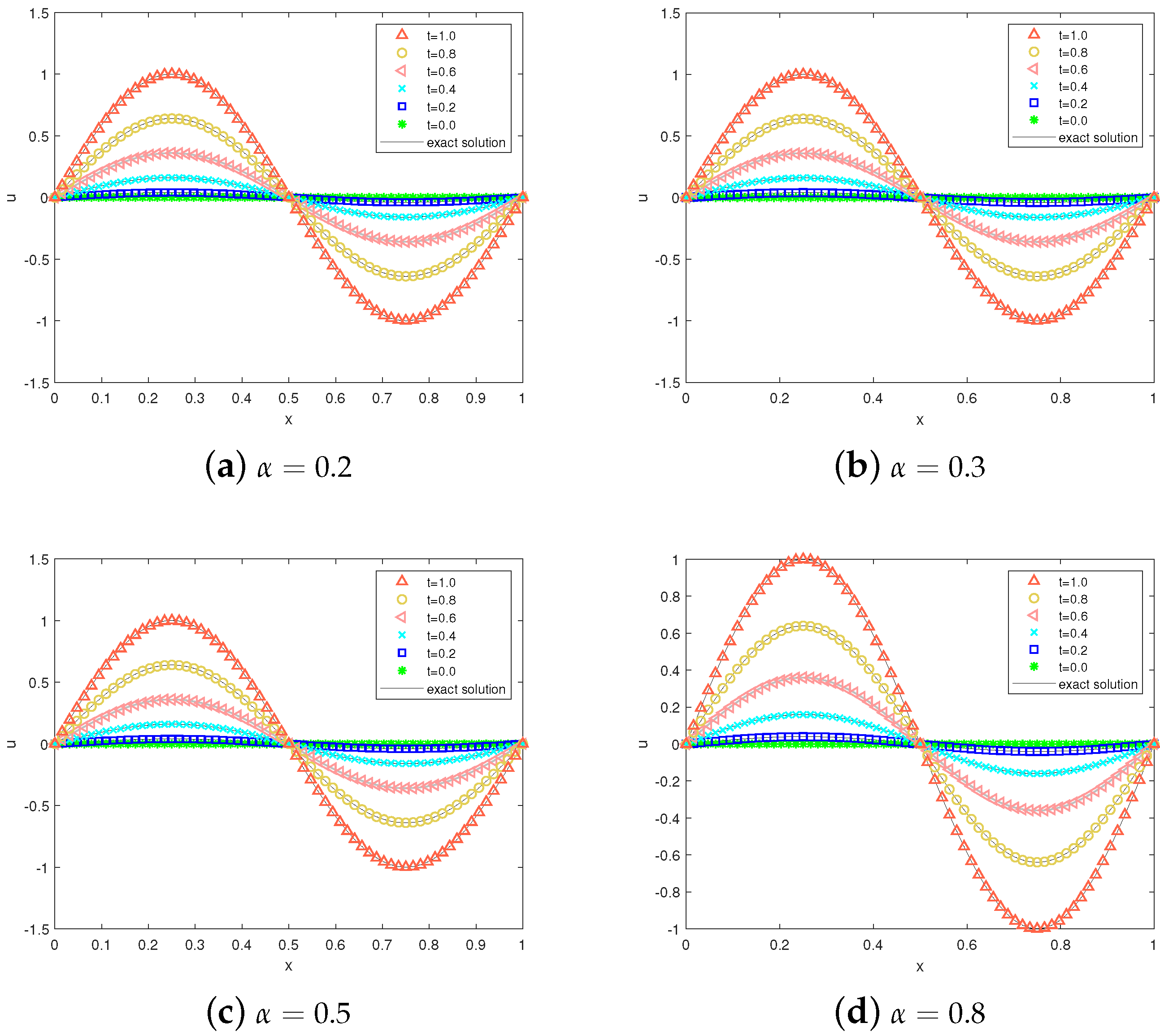
Example 3.
Consider the following time fractional Fisher’s problem [43],
0 C D t α u ( x , t ) Δ u ( x , t ) c u ( x , t ) 1 u d ( x , t ) = f ( x , t ) ( x , t ) L × [ 0 , 1 ]
u ( x , t ) t = 0 = 0 , 𝜕 u ( x , t ) 𝜕 t t = 0 = 0 , x L = [ 2 π , 2 π ]
with c = 1 , d = 1 and f ( x , t ) = 2 t ( 2 α ) / Γ ( 3 α ) + 2 t 2 t 4 sin ( x ) sin ( x ) . The exact solution of the problem is given by u ( x , t ) = t 2 s i n ( x ) .
In the computation, we take Δ t = 0.0002 , Δ x = 1 / 150 , τ = 1.15 , and α = 0.8 . Figure 6 shows the time evolution of the numerical solutions. Table 7 shows the GREs and MAEs with α = 0.4 , 0.5 , 0.8 , 0.9 for different lattice sizes. From Table 7, it can be seen that the errors decrease as the lattice size increases for different α .

4. Conclusions

In this paper, a lattice Boltzmann model with the auxiliary distribution function is proposed for the numerical solution of the FPDEs. Using the multiscale Chapman–Enskog expansion, the macroscopic equation with the second-order accuracy is recovered by choosing appropriate auxiliary distribution functions and equilibrium distribution functions. Numerical simulations are provided to verify the effectiveness of the proposed method. The numerical results are found to be in good agreement with the analytical solutions, and numerical accuracy is consistent with theoretical accuracy. Comparing the results between the numerical experiments for the sub-diffusion equation indicates that the present model achieves higher accuracy than the previous LB models. This proves that the proposed model demonstrates accuracy and efficiency in solving a class of FPDEs and can also be extended to solve more FPDEs. In addition, to solve more types of FPDEs, it would be an ongoing challenge to construct more efficient and accurate auxiliary distribution functions to recover the macroscopic term u in FPDEs. Nonetheless, further relevant research is still needed.

Author Contributions

Conceptualization, methodology, and validation, F.W. and C.L.; writing, software, and data curation, C.L.; formal analysis, F.W.; supervision, project administration, funding acquisition, review, and resources, Y.W. and N.H. All authors have read and agreed to the published version of the manuscript.

Funding

This work was supported by the National Natural Science Foundation of China (Grant No. 62103289) and the education department project of Liaoning Province (Grant No. LJKMZ20220485).

Institutional Review Board Statement

Not applicable.

Informed Consent Statement

Not applicable.

Data Availability Statement

Not applicable.

Conflicts of Interest

The authors declare no conflict of interest.

References

  1. Podlubnv, I. Fractional Differential Equations; Academic Press: San Diego, CA, USA; Boston, MA, USA, 1999; Volume 6. [Google Scholar]
  2. An, N.; Huang, C.; Yu, X. Error analysis of direct discontinuous Galerkin method for two-dimensional fractional diffusion-wave equation. Appl. Math. Comput. 2019, 349, 148–157. [Google Scholar] [CrossRef]
  3. Baillie, R.T. Long memory processes and fractional integration in econometrics. J. Econom. 1996, 73, 5–59. [Google Scholar] [CrossRef]
  4. Diethelm, K.; Ford, N.J. The Analysis of Fractional Differential Equations; Lecture Notes in Mathematics; Springer: Berlin/Heidelberg, Germany, 2010; Volume 2004, pp. 3–12. [Google Scholar]
  5. Kilbas, A.A.; Srivastava, H.M.; Trujillo, J.J. Theory and Applications of Fractional Differential Equations; Elsevier: Amsterdam, The Netherlands, 2006. [Google Scholar]
  6. Mainardi, F. Fractional Calculus: Some Basic Problems in Continuum and Statistical Mechanics; Springer: Vienna, Austria, 1997. [Google Scholar]
  7. Shymanskyi, V.; Sokolovskyy, I.; Sokolovskyy, Y.; Bubnyak, T. Variational Method for Solving the Time-Fractal Heat Conduction Problem in the Claydite-Block Construction. In Advances in Computer Science for Engineering and Education. ICCSEEA 2022; Lecture Notes on Data Engineering and Communications Technologies; Hu, Z., Dychka, I., Petoukhov, S., He, M., Eds.; Springer: Cham, Switzerland, 2022; Volume 134. [Google Scholar] [CrossRef]
  8. AlBaidani, M.M.; Ganie, A.H.; Aljuaydi, F. Application of Analytical Techniques for Solving Fractional Physical Models Arising in Applied Sciences. Fractal Fract. 2023, 7, 584. [Google Scholar] [CrossRef]
  9. Abdulwasaa, M.A.; Abdo, M.S.; Shah, K. Fractal-fractional mathematical modeling and forecasting of new cases and deaths of COVID-19 epidemic outbreaks in India. Results Phys. 2021, 20, 103702. [Google Scholar] [CrossRef]
  10. Yuste, S.B.; Acedo, L. Some exact results for the trapping of subdiffusive particles in one dimension. Phys. A 2004, 336, 334–346. [Google Scholar] [CrossRef]
  11. Fisher, R.A. The wave of advance of advantageous genes. Ann. Eugen. 1937, 7, 355–369. [Google Scholar] [CrossRef]
  12. Wei, Y.; Ullah, G.; Schiff, S.J. Unification of neuronal spikes, seizures, and spreading depression. J. Neurosci. 2014, 34, 11733–11743. [Google Scholar] [CrossRef] [PubMed]
  13. Strassberg, A.F.; DeFelice, L.J. Limitations of the Hodgkin-Huxley formalism: Effects of single channel kinetics on transmembrane voltage dynamics. Neural Comput. 1993, 5, 843–855. [Google Scholar] [CrossRef]
  14. Liu, F.; Anh, V.V.; Turner, I.; Zhuang, P. Time fractional advection-dispersion equation. J. Appl. Math. Comput. 2003, 13, 233–245. [Google Scholar] [CrossRef]
  15. Schneider, W.R.; Wyss, W. Fractional diffusion and wave equations. J. Appl. Math. Comput. 1989, 30, 134–144. [Google Scholar] [CrossRef]
  16. Liu, F.; Shen, S.; Anh, V. Analysis of a discrete non-Markovian random walk approximation for the time fractional diffusion equation. Anziam J. 2004, 46, C488–C504. [Google Scholar] [CrossRef]
  17. Sun, Z.; Wu, X. A fully discrete difference scheme for a diffusion-wave system. Appl. Numer. Math. 2006, 56, 193–209. [Google Scholar] [CrossRef]
  18. Gu, Y.; Zhuang, P.; Liu, F. An advanced implicit meshless approach for the non-linear anomalous subdiffusion equation. CMES Comp. Model. Eng. Sci. 2010, 56, 303–333. [Google Scholar]
  19. Liu, Q.; Gu, Y.; Zhuang, P. An implicit RBF meshless approach for time fractional diffusion equations. Comput. Mech. 2011, 48, 1–12. [Google Scholar] [CrossRef]
  20. Liu, Q.; Liu, F.; Turner, I. Finite element approximation for a modified anomalous subdiffusion equation. Appl. Math. Model. 2011, 35, 4103–4116. [Google Scholar] [CrossRef]
  21. Li, X.; Xu, C. A space-time spectral method for the time fractional diffusion equation. SIAM J. Numer. Anal. 2009, 47, 2108–2131. [Google Scholar] [CrossRef]
  22. Zheng, M.; Liu, F.; Turner, I. A novel high order space-time spectral method for the time fractional Fokker-Planck equation. SIAM J. Sci. Comput. 2015, 37, A701–A724. [Google Scholar] [CrossRef]
  23. Zidan, A.M.; Khan, A.; Shah, R. Evaluation of time-fractional Fisher’s equations with the help of analytical methods. Aims Math. 2022, 7, 18746–18766. [Google Scholar] [CrossRef]
  24. Kbiri, M.; Nonlaopon, K.; Zidan, M. Analytical investigation of fractional-order Cahn-Hilliard and gardner equations using two novel techniques. Mathematics 2022, 10, 1643. [Google Scholar] [CrossRef]
  25. Naeem, M.; Yasmin, H.; Shah, R. Investigation of Fractional Nonlinear Regularized Long-Wave Models via Novel Techniques. Symmetry 2023, 15, 220. [Google Scholar] [CrossRef]
  26. Higuera, F.J.; Jimnez, J. Boltzmann approach to lattice gas simulations. Europhys. Lett. 1989, 9, 663–668. [Google Scholar] [CrossRef]
  27. Chen, S.; Doolen, G. Lattice Boltzmann method for fluid flows. Annu. Rev. Fluid Mech. 1998, 3, 329–364. [Google Scholar] [CrossRef]
  28. Zhang, J.; Yan, G.; Shi, X. Lattice Boltzmann model for wave propagation. Phys. Rev. E 2009, 80, 026706. [Google Scholar] [CrossRef] [PubMed]
  29. Velivelli, A.C.; Bryden, K.M. Parallel performance and accuracy of lattice Boltzmann and traditional finite difference methods for solving the unsteady two-dimensional Burger’s equation. Phys. A 2006, 362, 139–145. [Google Scholar] [CrossRef]
  30. Zhang, J.; Yan, G. A lattice Boltzmann model for the Korteweg-de Vries equation with two conservation laws. Comput. Phys. Commun. 2009, 180, 1054–1062. [Google Scholar] [CrossRef]
  31. Liu, B.; Shi, W. A Non-Equilibrium Interpolation Scheme for IB-LBM Optimized by Approximate Force. Axioms 2023, 12, 298. [Google Scholar] [CrossRef]
  32. Liu, B.; Shi, W. An Explicit-Correction-Force Scheme of IB-LBM Based on Interpolated Particle Distribution Function. Entropy 2023, 25, 526. [Google Scholar] [CrossRef] [PubMed]
  33. Ginzburg, I. Variably saturated flow described with the anisotropic lattice Boltzmann methods. J. Comput. Fluid 2006, 25, 831–848. [Google Scholar] [CrossRef]
  34. Wang, M.; Wang, J.; Chen, S. Roughness and cavitations effect on electro-osmotic flows in rough microchannels using the lattice Poisson-Boltzmann methods. J. Comput. Phys. 2007, 226, 836–851. [Google Scholar] [CrossRef]
  35. Palpacelli, S.; Succi, S. Quantum lattice Boltzmann simulation of expanding Bose-Einstein condensates in random potentials. Phys. Rev. E 2008, 77, 066708. [Google Scholar] [CrossRef] [PubMed]
  36. Yepez, J. Relativistic path integral as a lattice-based quantum algorithm. Quantum Inf. Process. 2005, 4, 471–509. [Google Scholar] [CrossRef]
  37. Zhang, J.; Yan, G. Lattice Boltzmann model for the complex Ginzburg-Landau equation. Phys. Rev. E 2010, 81, 066705. [Google Scholar] [CrossRef] [PubMed]
  38. Du, R.; Sun, D.; Shi, B.; Chai, Z. Lattice Boltzmann model for time sub-diffusion equation in Caputo sense. Appl. Math. Comput. 2019, 358, 80–90. [Google Scholar] [CrossRef]
  39. Zhang, J.; Yan, G. Lattice Boltzmann method for the fractional sub-diffusion equation. Int. J. Numer. Methods Fluids 2016, 80, 490–507. [Google Scholar] [CrossRef]
  40. Liang, H.; Zhang, C.; Du, R. Lattice Boltzmann method for fractional Cahn-Hilliard equation. Commun. Nonlinear Sci. Numer. Simul. 2020, 91, 105443. [Google Scholar] [CrossRef]
  41. Qian, Y.; Succi, S.; Orszag, S. Recent advances in lattice boltzmann computing. Annu. Rev. Comput. Phys. III 1995, 3, 195–242. [Google Scholar]
  42. Guo, Z.; Zheng, C.; Shi, B. Non-equilibrium extrapolation method for velocity and pressure boundary conditions in the lattice Boltzmann method. Chin. Phys. 2002, 11, 366. [Google Scholar]
  43. Zhang, X.; He, Y.; Wei, L. A fully discrete local discontinuous Galerkin method for one-dimensional time-fractional Fisher’s equation. Int. J. Comput. Math. 2014, 91, 2021–2038. [Google Scholar] [CrossRef]
Figure 1. The exact and numerical solutions at different time and α .
Axioms 12 00959 g001
Figure 2. Accuracy analysis for Example 1 at different time and α .
Axioms 12 00959 g002
Figure 3. The exact and numerical solutions at t = 1.0 along y = 0.25 for Example 2(a).
Axioms 12 00959 g003
Figure 4. The numerical solutions at t = 1.0 for Example 2(a).
Axioms 12 00959 g004
Figure 5. Contour plots of the numerical solution and error for Example 2(a).
Axioms 12 00959 g005
Figure 6. The time evolution of the numerical solutions for Example 3.
Axioms 12 00959 g006
Table 1. Errors of different methods for Example 1 at t = 1.0 .
α MPresent MethodMethod of DU [38]
GRE MAE MAE
0.3161.7544 × 10 6 6.1363 × 10 6 2.2998 × 10 3
324.8714 × 10 7 1.4962 × 10 6 2.6936 × 10 4
641.5164 × 10 7 4.0821 × 10 7 5.0138 × 10 5
1286.5658 × 10 8 1.7434 × 10 7 1.7731 × 10 5
0.5163.7669 × 10 6 1.1127 × 10 5 5.3515 × 10 3
326.8474 × 10 7 2.2799 × 10 6 7.6823 × 10 4
641.7924 × 10 7 2.2522 × 10 6 1.2016 × 10 4
1283.8702 × 10 7 1.4508 × 10 6 2.4977 × 10 5
0.8161.0894 × 10 4 3.3249 × 10 4 1.4932 × 10 2
323.6885 × 10 5 1.0992 × 10 4 3.2711 × 10 3
641.5597 × 10 5 4.1596 × 10 5 7.0640 × 10 4
1287.1372 × 10 6 1.8928 × 10 5 1.3470 × 10 4
1.0166.6591 × 10 4 1.8440 × 10 3 2.2417 × 10 2
322.4490 × 10 4 6.7023 × 10 4 6.6025 × 10 3
641.3522 × 10 4 3.6431 × 10 4 1.9798 × 10 3
1281.0616 × 10 4 2.8558 × 10 4 5.3120 × 10 4
Table 2. Errors for Example 1 at t = 1.0 with different lattice sizes and α .
α M GRE MAE
0.01168.0274 × 10 8 2.7868 × 10 7
326.9069 × 10 9 2.0893 × 10 8
487.5300 × 10 9 2.0523 × 10 8
0.05161.3933 × 10 7 4.8418 × 10 7
322.3479 × 10 8 7.0848 × 10 8
487.5422 × 10 10 2.0520 × 10 9
0.1162.4973 × 10 7 8.6881 × 10 7
325.4541 × 10 8 1.6508 × 10 7
481.6335 × 10 8 4.4543 × 10 8
Table 3. GREs and MAEs of different methods for Example 1 at t = 1.0 .
MPresent MethodMMethod of Zhang [39]
GRE MAE GRE MAE
1282.6974 × 10 5 6.9908 × 10 5 1706.418 × 10 3 1.582 × 10 2
Table 4. Errors of different methods for Example 2(a) at t = 1.0 .
α M × N Present MethodMethod of DU [38]
GRE MAE MAE
0.3 16 × 16 6.0864 × 10 3 5.1726 × 10 3 1.4926 × 10 2
32 × 32 2.4343 × 10 4 2.1413 × 10 4 1.6269 × 10 3
48 × 48 1.8666 × 10 5 2.6660 × 10 5 3.8336 × 10 4
64 × 64 6.7115 × 10 6 2.2162 × 10 5 1.2868 × 10 4
128 × 128 7.5001 × 10 5 6.9910 × 10 5 ————–
0.5 16 × 16 1.2182 × 10 2 1.0949 × 10 2 3.4334 × 10 2
32 × 32 1.7267 × 10 3 1.5440 × 10 3 4.9764 × 10 3
48 × 48 4.2174 × 10 4 3.8606 × 10 4 1.4985 × 10 3
64 × 64 8.4348 × 10 5 8.7063 × 10 5 6.3202 × 10 4
128 × 128 7.9122 × 10 5 7.3838 × 10 5 ————–
0.8 16 × 16 4.2584 × 10 2 3.6619 × 10 2 9.1759 × 10 2
32 × 32 5.9819 × 10 3 5.3586 × 10 3 2.1532 × 10 2
48 × 48 2.0374 × 10 3 1.8499 × 10 3 8.4413 × 10 3
64 × 64 9.2507 × 10 4 8.7302 × 10 4 4.3092 × 10 4
128 × 128 8.9203 × 10 5 8.5114 × 10 5 ————–
1.0 16 × 16 1.0489 × 10 1 8.3526 × 10 2 1.5758 × 10 1
32 × 32 1.4115 × 10 2 1.2270 × 10 2 5.0922 × 10 2
48 × 48 4.6832 × 10 3 4.4487 × 10 3 2.3927 × 10 2
64 × 64 2.1425 × 10 3 1.9626 × 10 3 1.3632 × 10 2
128 × 128 6.8370 × 10 5 6.4402 × 10 5 ————–
Table 5. Errors with different times and α for Example 2(a).
t α = 0.2 α = 0.3 α = 0.5 α = 0.8
MAEGREMAEGREMAEGREMAEGRE
0.59.8770 × 10 6 4.2907 × 10 5 9.3553 × 10 6 3.8874 × 10 5 1.1042 × 10 5 4.3162 × 10 5 1.7127 × 10 4 7.3419 × 10 4
1.02.3550 × 10 5 2.5891 × 10 5 2.2162 × 10 5 6.7115 × 10 6 8.7063 × 10 5 8.4348 × 10 5 8.7302 × 10 4 9.2507 × 10 4
1.54.8916 × 10 5 1.8381 × 10 5 3.2139 × 10 5 1.5601 × 10 5 2.8801 × 10 4 1.2841 × 10 4 2.1061 × 10 3 1.0243 × 10 3
2.08.5143 × 10 5 1.7360 × 10 5 5.3616 × 10 5 1.4635 × 10 5 5.7050 × 10 4 1.3603 × 10 4 3.9680 × 10 3 1.0892 × 10 3
Table 6. Errors of different methods for Example 2(b) at t = 1.0 .
M × N Present Method M × N Method of Zhang [39]
GRE MAE GRE MAE
170 × 170 7.5269 × 10 4 4.9622 × 10 3 170 × 170 1.362 × 10 3 8.212 × 10 2
Table 7. Errors for Example 3 at t = 1.0 with different lattice sizes and α .
α M GRE MAE
0.4601.8258 × 10 3 3.6547 × 10 3
907.2793 × 10 4 1.4472 × 10 3
1206.6440 × 10 4 1.7386 × 10 3
1505.4787 × 10 4 1.0451 × 10 3
0.5602.1512 × 10 3 3.6047 × 10 3
908.9675 × 10 4 1.5613 × 10 3
1203.0617 × 10 4 7.8740 × 10 4
1502.4886 × 10 4 4.2818 × 10 4
0.8602.5255 × 10 3 4.2296 × 10 3
901.0036 × 10 3 1.6916 × 10 3
1204.7435 × 10 4 8.3203 × 10 4
1502.2345 × 10 4 4.7212 × 10 4
0.9603.7523 × 10 3 5.8680 × 10 3
901.3023 × 10 3 2.2639 × 10 3
1205.9784 × 10 4 1.0861 × 10 3
1503.2469 × 10 4 5.8540 × 10 4
Disclaimer/Publisher’s Note: The statements, opinions and data contained in all publications are solely those of the individual author(s) and contributor(s) and not of MDPI and/or the editor(s). MDPI and/or the editor(s) disclaim responsibility for any injury to people or property resulting from any ideas, methods, instructions or products referred to in the content.

