Article

Study of Rotavirus Mathematical Model Using Stochastic and Piecewise Fractional Differential Operators

by
Nadiyah Hussain Alharthi
and
Mdi Begum Jeelani
*
Department of Mathematics and Statistics, College of Science, Imam Mohammad Ibn Saud Islamic University (IMSIU), Riyadh 11564, Saudi Arabia
*
Author to whom correspondence should be addressed.
Axioms 2023, 12(10), 970; https://doi.org/10.3390/axioms12100970
Submission received: 16 September 2023 / Revised: 9 October 2023 / Accepted: 11 October 2023 / Published: 16 October 2023

Abstract

:
This manuscript is related to undertaking a mathematical model (susceptible, vaccinated, infected, and recovered) of rotavirus. Some qualitative results are established for the mentioned challenging childhood disease epidemic model of rotavirus as it spreads across a population with a heterogeneous rate. The proposed model is investigated using a novel approach of fractal calculus. We compute the boundedness positivity of the solution of the proposed model. Additionally, the basic reproduction ratio and its sensitivity analysis are also performed. The global stability of the endemic equilibrium point is also confirmed graphically using some available values of initial conditions and parameters. Sufficient conditions are deduced for the existence theory, the Ulam–Hyers ( UH ) stability. Specifically, the numerical approximate solution of the rotavirus model is investigated using efficient numerical methods. Graphical presentations are presented corresponding to a different fractional order to understand the transmission dynamics of the mentioned disease. Furthermore, researchers have examined the impact of lowering the risk of infection on populations that are susceptible and have received vaccinations, producing some intriguing results. We also present a numerical illustration taking the stochastic derivative of the proposed model graphically. Researchers may find this research helpful as it offers insightful information about using numerical techniques to model infectious diseases.

1. Introduction

Rotavirus is the most frequent cause of severe diarrhea in children worldwide and is estimated to be responsible for 215,000 deaths in children under five each year according to a WHO report in 2008 (see [1]). The virus, which is a member of the reoviridae family, is classified into seven sero-types (G1–G7) according to the outer capsid protein ([2]). The rotavirus infection is extremely contagious and can be transmitted orally through feces. Symptoms include fever, vomiting, and diarrhea. Because the virus can persist in an environment for extended periods of time, it is challenging to contain using conventional sanitation techniques (see [3]). The concerned virus also infected adults and it has some history which has been demonstrated in (see [4,5]). One common cause of severe diarrhea in young children is rotavirus, which is particularly dangerous for newborns and young children under five years old. Frequent contact with feces, whether through respiratory droplets, infected items, water, or food is the main method of transmission. Since there is now no cure for rotavirus infection, immunization is still the most effective way to stop its spread. The dynamics of rotavirus outbreaks have been better understood using mathematical modeling, especially in relation to immunization. In addition to the mentioned disease of five common types, some research was conducted in 2020 (see [6]).
According to recent research, mathematical modeling can help in understanding the dynamics of rotavirus transmission, forecasting its consequences in specific nations, and assessing the possible outcomes of interventions. Technology has advanced epidemiology to the point where several infectious diseases are now examined for treatment, control, curing, and other outcomes. As a result, the mathematical modeling of infectious diseases has greatly advanced over the past few decades (see [7,8]). In the last thirty years, mathematical modeling has been used in research more and more. A number of diseases, including those mentioned in citations [9,10], can be effectively controlled by the use of mathematical models in secure public health systems. These mathematical models can be used to study spatiotemporal patterns as well as the dynamic behavior of infections. Researchers have studied rotavirus disease from a variety of angles during the past three years because of the significance of mathematical models. Researchers in this field are employing a variety of strategies to develop practical procedures for controlling this illness (a number of recent studies are listed in citations [11,12,13]). Recently, the effects of immunization in elderly homes were investigated using a mathematical model (see [14]). Scholars [15] investigated intervention strategies for the rotavirus pandemic and mathematical modeling. In all the mentioned studies, researchers have used classical or stochastic type models for their study.
To the best of our knowledge, the field of epidemiology has thoroughly examined the idea of the classical derivative. It is well known that a variety of inherited, long-term, and short-term memory processes can be explained by classical differential operators, which are short because of their local character. Fractional calculus has gained much more attention in recent years in an effort to better understand the previously outlined procedure. Due to its dynamic features, which have demonstrated a range of applications in real-world scenarios, including biological and physical processes, it has become more and more popular (see [16]). Fractional calculus has a long history, just like conventional calculus (see [17]). Numerous writers have examined the subject matter from different angles; some of them are included as [18,19]. Numerous scientific and technological fields employ the previously stated calculus (see [20,21]). Because it is non-local, the fractional order derivative has a greater degree of freedom (see [22]). Consequently, the aforementioned derivative may be selected above the standard order derivative in the mathematical modeling of infectious diseases. The existence theory of solutions to fractional differential equations in [23] and qualitative results in [24], respectively, are among the enlightening works that several writers have. In order to investigate fractional order differential and integral equations (FODIEs) for approximate or analytical results, a variety of tools and methods have been developed (see, for example, the fractional visco-elasticity model in [25]).
Most problems in the actual world are partially unpredictable, which is something that conventional mathematical models cannot explain. In recent decades, the concept of stochastic mathematical differential equations has been proposed and applied with impressive results. Some problems, on the other hand, show non-locality tendencies rather than randomness. These include crossover behaviors, fractal processes, power law processes, and long-range dependencies, which imply that physical phenomena display a range of behaviors. To solve these issues, a class of fractional derivatives was suggested. Still, these operators are not very good at characterizing crossover behavior. For the first time, the concept of short memory with real or complex order derivatives was created to describe the previously indicated behavior. To explain the above behavior, the concept of short memory fractional order derivatives was introduced for the first time (see [26]). To examine the crossover properties, we provide several notions: fractal–fractional derivative, fractional order derivative with singular and non-singular kernels, and several other derivative operator types. Though studies of stochastic equations lead to more realistic conclusions, the crossover dynamical behavior has not been addressed. Numerous real-world process models, such as those involving heat flow, fluid flow, and numerous intricate advection issues, exhibit this behavior. The exponential or Mittag–Leffler mappings cannot be used in fractional calculus to predict the timing of crossings because the typical fractional order derivative is unable to adequately capture the crossover behavior that is prevalent in real-world applications. Due to rapid changes in their state of rest or uniform motion, as well as natural occurrences like earthquakes, pendulum motion, the unstable status of the economy in less developed countries today, etc. Fractional order derivatives of piecewise equations provide an example of this crossover phenomenon. Recent work has identified certain critical components in this regard through the study of multiple models (see [27,28]). The authors developed classical and global piecewise derivatives in addition to a number of applications. We refer to [29] for the mentioned details.
Overall, rotavirus research conducted recently has brought to light the significance of mathematical modeling for understanding the dynamics of rotavirus transmission and for forecasting the possible outcomes of interventions. Furthermore, risk factors for severe rotavirus infection have been found in recent studies, which have also looked into new possibilities for diagnosis and therapy. Continued research in these areas is crucial in the fight against rotavirus and the reduction in deaths caused by this virus. For instance, authors [28] studied a compartmental model for the said disease under vaccination class as
S ˙ ( t ) = ( 1 ϑ ) μ κ S ( t ) I ( t ) + ς V ( t ) ( ρ + λ ) S ( t ) V ˙ ( t ) = ϑ μ + ρ S ( t ) ζ κ V ( t ) I ( t ) ( ς + λ ) V ( t ) I ˙ ( t ) = κ S ( t ) I ( t ) + ζ κ V ( t ) I ( t ) ( τ + ω + λ ) I ( t ) R ˙ ( t ) = ω I ( t ) λ R ( t ) S 0 > 0 , V 0 0 , I 0 0 , R 0 0 ,
where ( 1 ϑ ) μ and ϑ μ represent birth rates in the S and V classes, respectively. κ is the infection rate of S, and an individual is vaccinated from S at the rate denoted by ρ . Further, the vaccine is imperfect and is assumed to wane at the rate ς . Furthermore, the parameter ζ ( 0 , 1 ) represents the expected decrease in the risk of infection as a result of vaccination. Moreover, the induced rate of disease is given by τ , and natural death rate is λ . Furthermore, the rate of recovery is represented by ω .
Keeping in mind the usefulness of piecewise derivatives, we extended the Model (1) to the following form
0 P C C D t p ( S ) ( t ) = ( 1 ϑ ) μ κ S ( t ) I ( t ) + ς V ( t ) ( ρ + λ ) S ( t ) 0 P C C D t p ( V ) ( t ) = ϑ μ + ρ S ( t ) ζ κ V ( t ) I ( t ) ( ς + λ ) V ( t ) 0 P C C D t p ( I ) ( t ) = κ S ( t ) I ( t ) + ζ κ V ( t ) I ( t ) ( τ + ω + λ ) I ( t ) 0 P C C D t p ( R ) ( t ) = ω I ( t ) λ R ( t ) ,
where 0 P C C D t p stands for the piecewise Caputo derivative which can be described by dividing the interval [ 0 , T ] into two subintervals at point t 1 as [ 0 , t 1 ] , and ( t 1 , T ] , respectively, for a differentiable function; say S as
0 P C C D t p ( S ( t ) ) = 0 C D t ( S ( t ) ) = S ˙ ( t ) , 0 < t t 1 , 0 C D t p ( S ( t ) ) = 1 Γ ( 1 p ) t 1 t ( t η ) p S ( η ) d η , t 1 < t T .
Here, it should be kept in mind that to capture crossover behavior, we can divide the interval [ 0 , T ] , T < into several intervals. In addition, t 1 is a fixed value. Here, the schematic diagram of our model is given in Figure 1.
The feasible zone is ascertained once the boundednessfor the presence of the solution is confirmed. Then, using the Banach and Schauder fixed-point theorems, the existence and uniqueness of approximation solutions for the previously described model are examined. Notably, existence theory with piecewise derivatives of fractional orders offers some novel insights into such dynamical issues. According to the hypothesis, it is possible to solve these kinds of physical issues. Numerous numerical methods have been shown to be especially effective for classical fractional order systems in recent years. One of the most effective numerical techniques is the Runge–Kutta method with reliable step size information.The Range-Kutta approach, for example, was used for several fractional order problems in [30]. Furthermore, the results devoted to UH stability are also derived. The concerned stability is investigated for the best approximate or exact solution [31]. The existence theory is established using fixed-point approaches as mentioned in [32,33].
It is amazing how random events affect everything in the real world, even the movements of people and animals. Some interesting work on different biological models can be studied in [34,35,36,37,38,39,40]. This impact is mathematically interpreted in terms of stochastic models. These previously mentioned notions have been used to examine mathematical models. It is important to note that stochastic calculus has important applications in simulating real-world processes. Because of this, academics have recently looked into a few mathematical models using the previously described field (see [41,42]). A growing number of additional infectious diseases have also been modeled using the aforementioned differential equations (see [43,44]). Driven by the aforementioned significance of stochastic calculus, we also endeavor to replicate the suggested Model (3) under the stochastic white noise as
d S ( t ) = ( 1 ϑ ) μ κ S ( t ) I ( t ) + ς V ( t ) ( ρ + λ ) S ( t ) d t + σ 1 S ( t ) d β 1 ( t ) d E ( t ) = ϑ μ + ρ S ( t ) ζ κ V ( t ) I ( t ) ( ς + λ ) V ( t ) d t + σ 2 V ( t ) d β 2 ( t ) d I ( t ) = κ S ( t ) I ( t ) + ζ κ V ( t ) I ( t ) ( τ + ω + λ ) I ( t ) d t + σ 3 I ( t ) d β 3 ( t ) d R ( t ) = ω I ( t ) λ R ( t ) d t + σ 4 R ( t ) d β 4 ( t ) ,
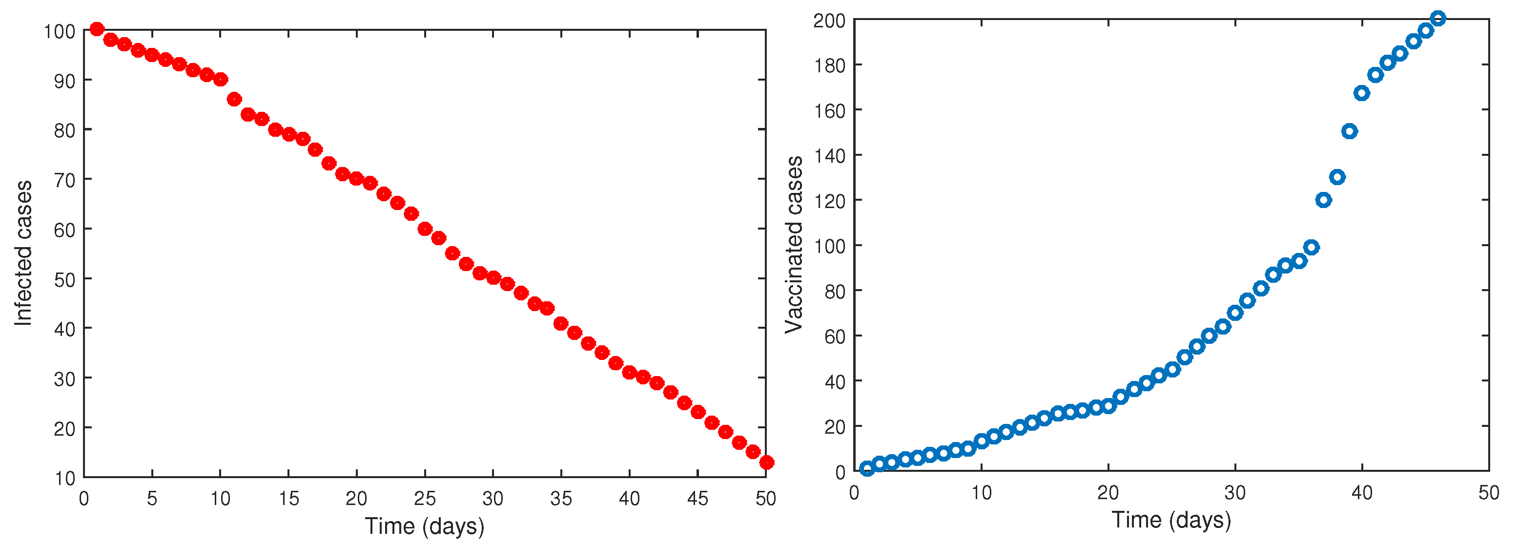
where β i denote Brownian motion with β i ( 0 ) = 0 , and σ i > 0 , for i = 1, 2, 3, 4 denote the intensity of white noise. Here, it should be kept in mind that we will simulate our Model (3) using the numerical scheme developed in [45,46]. Researchers have worked on collecting some real data cases for both infected and vaccinated people [47] in Saudi Arabia, and we present the graphical presentation of the aforesaid cases in Figure 2. In Saudi Arabia, rotavirus infection is a substantial contributor to childhood morbidity.
This text is organized as follows: Part 1 contains a thorough introduction to our work. In Section 2, there are a few essential outcomes that we require for this work. Some of the basic results of the proposed model are also presented here. In Section 3, we use a fixed-point theory to build an existence theory for a rough solution to the suggested model. The numerical method for an approximate solution to the proposed model is covered in Section 4. We provide examples to support our conclusions in Section 5. In conclusion, Section 6 provides a succinct overview and clarification of the numerical results.

2. Elementary Results

Recollecting some basic results as follow:
Definition 1
([29]). If ϱ be a differentiable function with p > 0 , then a piecewise integral is described by considering J = [ 0 , T ] , J 1 = [ 0 , t 1 ] , J 2 = ( t 1 , T ] as
0 P C I t p ϱ ( t ) = 0 t 1 ϱ ( ν ) d ν , t J 1 , 1 Γ ( p ) t 1 t ( t ν ) p 1 ϱ ( ν ) d ( ν ) , t J 2 ,
where 0 P C I t stands for classical integration in J 1 and represents Riemann–Liouville integration in J 2 .
Definition 2
([29]). Let 0 < p 1 and if ϱ C ( J ) be differentiable, then the classical and fractional order piecewise derivative is defined as
0 P C C D t p ϱ ( t ) = ϱ ˙ ( t ) , t J 1 , 0 C D t p ϱ ( t ) , t J 2 .
Lemma 1
([29]). Let ϱ L ( J ) C ( J ) and ψ L ( J ) , then the solution of the given problem
0 P C C D t p ϱ ( t ) = ψ ( t ) , 0 < p 1
is derived as
ϱ ( t ) = ϱ 0 + 0 t ψ ( ν ) d ν , t J 1 , ϱ ( t 1 ) + 1 Γ ( p ) t 1 t ( t ν ) p 1 ψ ( ν ) d ( ν ) , t J 2 .

2.1. Some Fundamental Results about the Model (3)

About the Model (3), we derive some axillary results. The feasible region is given in Remark 1.
Remark 1.
Let N be the total population at any time t, then
N = S + V + I + R .
Applying a piecewise derivative of (4) w.r.t ′t′ from Model (3), we obtain
0 P C C D t p N ( t ) = λ μ N ,
which in taking the Laplace transform and using t yields
N ( t ) λ μ .
Thus, the feasible region is given by
Ω = ( S , V , I , R ) R + 4 : N λ μ .

2.2. Equilibrium Points and Basic Reproduction Number

Putting the left-hand sides of Model (3) equal to zero and solving the equations, the disease-free equilibrium is obtained. From Model (3), one has
( 1 ϑ ) μ κ S ( t ) I ( t ) + ς V ( t ) ( ρ + λ ) S ( t ) = 0 ϑ μ + ρ S ( t ) ζ κ V ( t ) I ( t ) ( ς + λ ) V ( t ) = 0 κ S ( t ) I ( t ) + ζ κ V ( t ) I ( t ) ( τ + ω + λ ) I ( t ) = 0 ω I ( t ) λ R ( t ) = 0 ,
on solving in a disease-free equilibrium state when I 0 = 0 is given by S 0 = ( 1 ϑ ) μ ρ + λ , V 0 = ϑ μ ( ρ + λ ) + ( 1 ϑ ) μ ρ + λ , I 0 = 0 , R 0 = 0 . Hence, local equilibrium is given by
E 0 = ( S 0 , 0 , 0 , 0 ) = ( 1 ϑ ) μ ρ + λ , ϑ μ ( ρ + λ ) + ( 1 ϑ ) μ ρ + λ , 0 , 0 .
Furthermore, the endemic equilibrium E * = ( S * , V * , I * , R * ) is computed as
S * = ζ κ ( a ϑ μ ( τ + ω + λ ) I * ( τ + ω + λ ) ( ζ ϑ μ ( τ + ω + λ ) I * ) κ ( ζ κ 2 I * + κ ( ς + λ ) ζ κ ) , V * ( t ) = κ ϑ μ ( τ + ω + λ ) I * ζ κ 2 I * + κ ( ς + λ ) ζ κ ) , I * = κ ( 1 ϑ ) μ ( ς + λ ρ ζ ) + ζ ( κ ϑ μ ρ ( τ + ω + λ ) ) ζ ( ρ + λ ) ( κ ϑ μ ρ ( ρ + λ ) ) ( ρ + λ ) ( τ + ω + λ ) ( ς + λ ρ ζ ) κ 2 ( 1 ϑ ) μ ζ ζ κ ( κ ϑ μ ρ ( τ + ω + λ ) ) ( ρ + λ ) ( τ + ω + λ ) ζ κ , R * = ω I * λ .
In addition, the fundamental reproductive number can be computed as R 0 = μ κ λ ( τ + ω + λ ) . Clearly, if R 0 < 1 , the trivial equilibrium point is called locally asymptotically stable. Now, the 3D profile of R 0 is given in Figure 3.
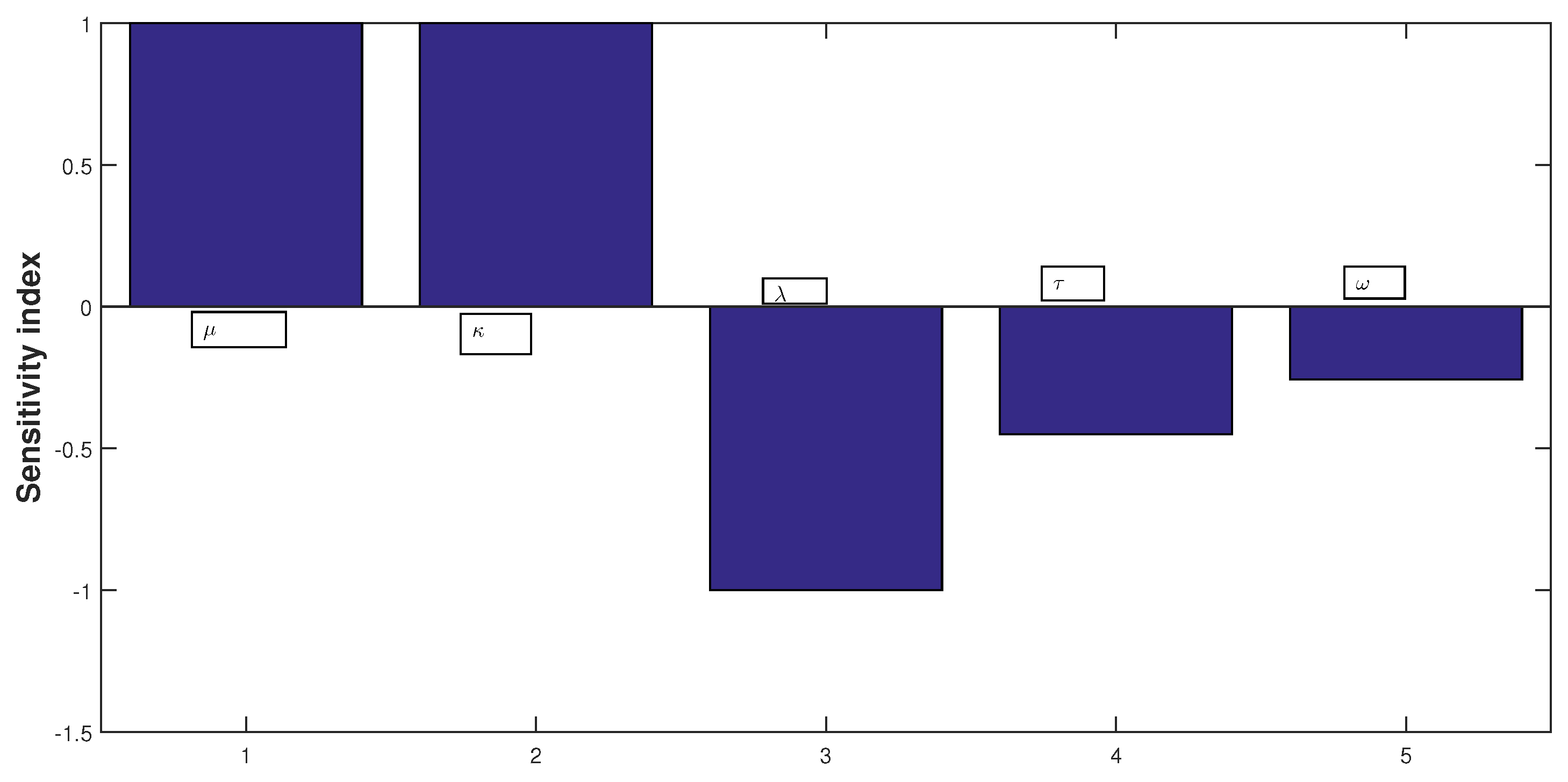
Calculations are made to determine the reproductive number R 0 and sensitivity indices to the model parameters. These indices show the significance of each aspect in the spread and incidence of disease. Sensitivity analysis is used to evaluate the model predictions’ resistance to parameter values. In this regard, we use the following formula for the computation of sensitivity indices
S q R 0 = q R 0 R 0 q .
Using Formula (6), we have
S μ R 0 = μ R 0 R 0 μ = 1 > 0 , S κ R 0 = κ R 0 R 0 κ = 1 > 0 , S λ R 0 = λ R 0 R 0 λ = ( 2 λ + τ + ω ) τ + ω + λ < 0 , S τ R 0 = τ R 0 R 0 τ = τ τ + ω + λ < 0 , S ω R 0 = ω R 0 R 0 ω = ω λ + ω + λ < 0 .
In Figure 4, we present the sensitivity index against the given parameters of the proposed Model (3).
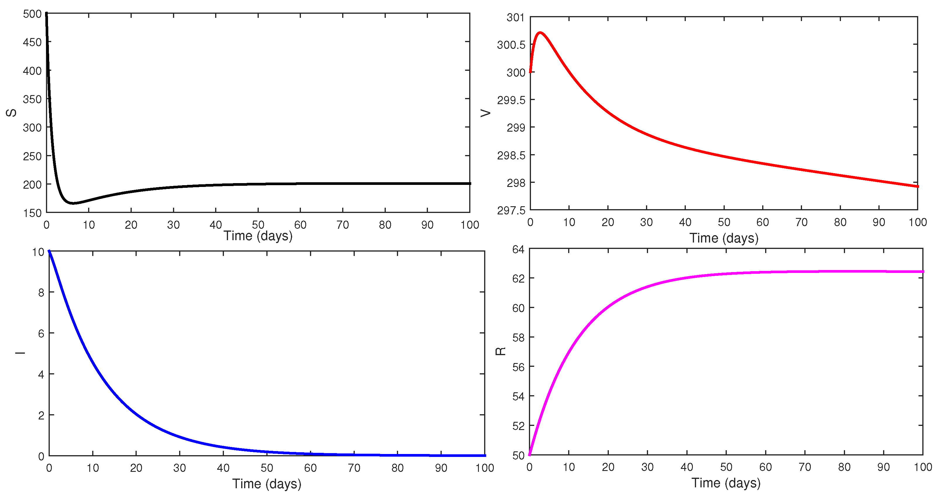
In addition, using the parameter values given in Table 1, we have R 0 = 1.6213 > 1 , which implies that the endemic equilibrium E * = ( S * , V * , I * , R * ) of Model (3) is globally asymptotically stable. The concerned stability has been shown in Figure 5.

3. Existence Theory

Here, we develop sufficient results for the qualitative theory of existence and uniqueness using a fixed-point approach. Here, we write the right sides of our proposed Model (3) using ϱ = ( S , V , I , R ) as
0 P C C D t p ( S ) ( t ) = W 1 ( t , ϱ ( t ) ) 0 P C C D t p ( V ) ( t ) = W 2 ( t , ϱ ( t ) ) 0 P C C D t p ( I ) ( t ) = W 3 ( t , ϱ ( t ) ) 0 P C C D t p ( R ) ( t ) = W 4 ( t , ϱ ( t ) ) ,
and ϱ 0 = ( S 0 , V 0 , I 0 , R 0 ) .
One alternative format for the equation including the piecewise Caputo derivative is considered as
0 P C C D t p ϱ ( t ) = W ( t , ϱ ( t ) ) , 0 < p 1 , ϱ ( 0 ) = ϱ 0 ,
where W : J × R R is a nonlinear continuous function. The solution using Lemma 1 is computed as
ϱ ( t ) = ϱ 0 + 0 t W ( ν , ϱ ( ν ) ) d ν , t J 1 , ϱ ( t 1 ) + 1 Γ ( p ) t 1 t ( t ν ) p 1 W ( ν , ϱ ( ν ) ) d ( ν ) , t J 2 ,
Let T < , the Banach space is defined as X = C ( J ) × C ( J ) × C ( J ) × C ( J ) under the norm
ϱ = max t J | ϱ ( t ) | .
These hypotheses hold for further results.
(C1)
If Δ W > 0 is constant, such that ϱ , ϱ ¯ X , then
| W ( t , ϱ ) W ( t , ϱ ¯ ) | Δ W | ϱ ϱ ¯ | .
(C2)
For constants Λ W > 0 and Υ W > 0 , we have
| W ( t , ϱ ( t ) ) | Λ W | ϱ | + Υ W .
Theorem 1.
For the assumed function W defined in (17), which is a piecewise continuous on J 1 and J 2 which are subintervals of J , and the assumptions ( C 1 ) , ( C 2 ) hold, then the problem (17) has at least one solution. Consequently, Model (3) has at least one solution.
Proof. 
Let Θ = { ϱ X : ϱ J 1 , 2 , J 1 , 2 > 0 } be a closed and bounded subset of X , where
J 1 , 2 max | ϱ 0 | + t 1 Υ W 1 t 1 Λ W , t J 1 , | ϱ ( t 1 ) | Γ ( p + 1 ) + T p Υ W ( Γ ( p + 1 ) T p Λ W , t J 2 .
If N : Θ Θ be the operator defined as
N ( ϱ ) = ϱ 0 + 0 t W ( ν , ϱ ( ν ) ) d ν , t J 1 , ϱ ( t 1 ) + 1 Γ p t 1 t ( t ν ) σ 1 W ( ν , ϱ ( ν ) ) d ( ν ) , t J 2 .
For ϱ Θ , we have
| N ( ϱ ) ( t ) | | ϱ 0 | + 0 t 1 | W ( ν , ϱ ( ν ) ) | d ν , | ϱ ( t 1 ) | + 1 Γ ( p ) t 1 t ( t ν ) p 1 | W ( ν ϱ ( ν ) ) | d ( ν ) , | ϱ 0 | + 0 t 1 [ Λ W | ϱ | + Υ W ] d ν , | ϱ ( t 1 ) | + 1 Γ ( p ) t 1 t ( t ν ) p 1 [ Λ W | ϱ | + Υ W ] d ( ν ) , | ϱ 0 | + t 1 [ Λ W J 1 , 2 + Υ W ] J 1 , 2 , t J 1 , | ϱ ( t 1 ) | + T p Γ ( p + 1 ) [ Λ W J 1 , 2 + Υ W ] J 1 , 2 , t J 2 ,
where for t J 2 , we put | ( t 1 ν ) p ( t 2 ν ) p | T p . Hence, we have that N ( ϱ ) J 1 , 2 which yields N ( Θ ) Θ . Thus, N maps are set to bounded.Thus, N is a bounded operator. Since W is a continuous function, therefore N is also a continuous operator. Next, for complete continuity, consider t m < t n J 1 , then
| N ( ϱ ) ( t n ) N ( ϱ ) ( t m ) | = | 0 t n W ( ν , ϱ ( ν ) ) d ν 0 t m W ( ν , ϱ ( ν ) ) d ν | t m t n | W ( ν , ϱ ( ν ) ) | d ν t m t n [ Λ W | ϱ | + Υ W ] d ν ( Λ W J 1 , 2 + Υ W ) [ t n t m ] .
From (11), we see that t m t n , then
| N ( ϱ ) ( t n ) N ( ϱ ) ( t m ) | 0 , as t m t n .
Furthermore, N is a bounded operator. So
N ( ϱ ) ( t n ) N ( ϱ ) ( t m ) 0 , as t m t n .
Hence, N is equi-continuous in this case. In addition, take t m < t n J 2 and consider
| N ( ϱ ) ( t n ) N ( ϱ ) ( t m ) | = | 1 Γ ( p ) 0 t n ( t n ν ) p 1 W ( ν , ϱ ( ν ) ) d ν 1 Γ ( p ) 0 t m ( t m ν ) p 1 W ( ν , ϱ ( ν ) ) d ν | 1 Γ ( p ) 0 t m [ ( t m ν ) p 1 ( t n ν ) p 1 ] | W ( ν , ϱ ( ν ) ) | d ν + 1 Γ ( p ) t m t n ( t n ν ) p 1 | W ( ν , ϱ ( ν ) ) | d ν 1 Γ ( p ) [ 0 t m [ ( t m ν ) p 1 ( t n ν ) p 1 ] d ν + t m t n ( t n ν ) p 1 d ν ] ( Λ W | ϱ | + Υ W ) ( Λ W J 1 , 2 + Υ W ) Γ ( p + 1 ) [ t n p t m p + 2 ( t n t m ) p ] .
Further, from (12), we see that
| N ( ϱ ) ( t n ) N ( ϱ ) ( t m ) | 0 , as t m t n .
Furthermore, N is bounded over J 2 so it is uniformly continuous. Hence,
N ( ϱ ) ( t n ) N ( ϱ ) ( t m ) 0 , as t m t n .
Therefore, N is equi-continuous in a J 2 interval. Hence, N is an equi-continuous mapping over J 1 J 2 . Thus, N is a relatively compact operator. By using the Arzelá–Ascoli theorem stated in [32], operator N is completely continuous. Therefore, Schauder’s fixed-point theorem is given in [33], and the concerned problem (17) has at least one solution. Hence, in view of the above results, we conclude that the proposed Model (3) has at least one solution. □
Theorem 2.
If assumption ( C 1 ) and the condition max t 1 Δ W , T p Γ ( p + 1 ) Δ W < 1 , hold, then the problem (17) has a unique solution in both subintervals J 1 and J 2 .
Proof. 
Let N : X X be the mapping defined as
N ( ϱ ) = ϱ 0 + 0 t W ( ν , ϱ ( ν ) ) d ν , t J 1 , ϱ ( t 1 ) + 1 Γ p t 1 t ( t ν ) σ 1 W ( ν , ϱ ( ν ) ) d ( ν ) , t J 2 .
Let ϱ , ϱ ¯ X , then over J 1 , one has
N ( ϱ ) N ( ϱ ¯ ) = max t J 1 | 0 t W ( ν , ϱ ( ν ) ) d ν 0 t 1 W ( ν , ϱ ¯ ( ν ) ) d ν | t 1 Δ W ϱ ϱ ¯ .
From (13), we have
N ( ϱ ) N ( ϱ ¯ ) t 1 Δ W ϱ ϱ ¯ .
By the same fashion for t J 2 , we have
N ( ϱ ) N ( ϱ ¯ ) = max t J 2 | 1 Γ ( p ) t 1 t ( t ν ) p 1 W ( ν , ϱ ( ν ) ) d ν 1 Γ ( p ) t 1 t ( t ν ) p 1 W ( ν , ϱ ¯ ( ν ) ) d ν | T p Γ ( p + 1 ) Δ W ϱ ϱ ¯ .
From (15), we have
N ( ϱ ) N ( ϱ ¯ ) T p Γ ( p + 1 ) Δ W ϱ ϱ ¯ .
Hence, from (14) and (16), we see that N is a contraction operator. Hence, (17) has a unique solution in both subintervals J 1 and J 2 . From the aforesaid results, we follow that the proposed Model (2) has a unique solution. □
Remark 2.
Let there exist a non-decreasing function π C ( J ) , such that
( i )
| π ( t ) | ε , t J .
In addition, the solution of the problem
0 P C C D t p ϱ ( t ) = W ( t , ϱ ) + π ( t ) , 0 < p 1 , ϱ ( 0 ) = ϱ 0
is given as
ϱ ( t ) = ϱ 0 + 0 t W ( ν , ϱ ( ν ) ) d ν + 0 t π ( ν ) d ν , t J 1 , ϱ ( t 1 ) + 1 Γ ( p ) t 1 t ( t ν ) p 1 W ( ν , ϱ ( ν ) ) d ( ν ) + 1 Γ ( p ) t 1 t ( t ν ) p 1 π ( ν ) d ( ν ) , t J 2 ,
In view of ( i ) , we have from (18) that
| ϱ ( t ) ϱ 0 + 0 t W ( ν , ϱ ( ν ) ) d ν | ε t 1 , i f t J 1 ,
and
| ϱ ( t ) ϱ ( t 1 ) + 1 Γ ( p ) t 1 t ( t ν ) p 1 W ( ν , ϱ ( ν ) ) d ( ν ) | + ε t 1 Γ ( p + 1 ) , i f t J 2 .
Theorem 3.
If the assumption ( C 1 ) and the condition max Δ W t 1 , ε t 1 Δ W Γ ( p + 1 ) < 1 hold, then the solution of problem (17) is UH stable over both subintervals J 1 and J 2 .
Proof. 
Let ϱ be any solution of (17), for which we have a unique solution ϱ ^ , then for t J 1 , one has by using Remark 2,
| ϱ ( t ) ϱ ^ ( t ) | = | ϱ ( t ) ϱ 0 + 0 t W ( ν , ϱ ^ ( ν ) ) d ν | | ϱ ( t ) ϱ 0 + 0 t W ( ν , ϱ ( ν ) ) d ν | + | 0 t W ( ν , ϱ ( ν ) ) d ν 0 t W ( ν , ϱ ^ ( ν ) ) d ν | ε t 1 + Δ W t 1 ϱ ϱ ^ ,
which further yields that
ϱ ϱ ^ ε t 1 1 Δ W t 1 .
In the same way, if t J 2 , repeating the same process, one has
ϱ ϱ ^ ε t 1 Γ ( p + 1 ) 1 ε t 1 Δ W Γ ( p + 1 ) .
Hence, from (21) and (22), we have that the solution is UH stable over both subintervals J 1 and J 2 . In view of the above results, the solution of the proposed Model (3) is also UH stable. □

4. Numerical Scheme

For the numerical presentation of Model (3), we construct a numerical method for the two subintervals of J . The numerical scheme for the piecewise problem well is like an integer order numerical scheme as established in [46] by using ϱ = ( S , V , I , R ) , as
S ( t n + 1 ) = S n 1 ( t n 1 ) + h 2 W 1 t n 1 + h 2 , ϱ n 1 ( t n 1 ) + M 1 2 , t I 1 , S n ( t n ) + h p Γ ( p + 1 ) W 1 ( t n , ϱ n ( t n ) ) + h p 2 Γ ( p + 1 ) M 2 + M 3 , t I 2 ,
where h = t n + 1 t n , and
M 1 = W 1 ( t n 1 , ϱ n 1 ( t n 1 ) ) , M 2 = W 1 ( t n , ϱ n ( t n ) ) , M 3 = W 1 t n + 2 h p Γ ( p + 1 ) Γ ( 2 p + 1 ) , ϱ ( t n ) + 2 h p Γ ( p + 1 ) Γ ( 2 p + 1 ) W 1 ( t n , ϱ n ( t n ) ) .
In the same way, we can establish for other compartments as given by
V ( t n + 1 ) = S n 1 ( t n 1 ) + h 2 W 2 t n 1 + h 2 , ϱ n 1 ( t n 1 ) + M 1 2 , t I 1 , V n ( t n ) + h p γ ( p + 1 ) W 2 ( t n , ϱ n ( t n ) ) + h p 2 Γ ( p + 1 ) M 2 + M 3 , t I 2 ,
I ( t n + 1 ) = S n 1 ( t n 1 ) + h 2 W 3 t n 1 + h 2 , ϱ n 1 ( t n 1 ) + M 1 2 , t I 1 , I n ( t n ) + h p γ ( p + 1 ) W 3 ( t n , ϱ n ( t n ) ) + h p 2 Γ ( p + 1 ) M 2 + M 3 , t I 2 ,
and for the last class as
R ( t n + 1 ) = S n 1 ( t n 1 ) + h 2 W 4 t n 1 + h 2 , ϱ n 1 ( t n 1 ) + M 1 2 , t I 1 , R n ( t n ) + h p γ ( p + 1 ) W 4 ( t n , ϱ n ( t n ) ) + h p 2 Γ ( p + 1 ) M 2 + M 3 , t I 2 .

5. Simulations and Discussion

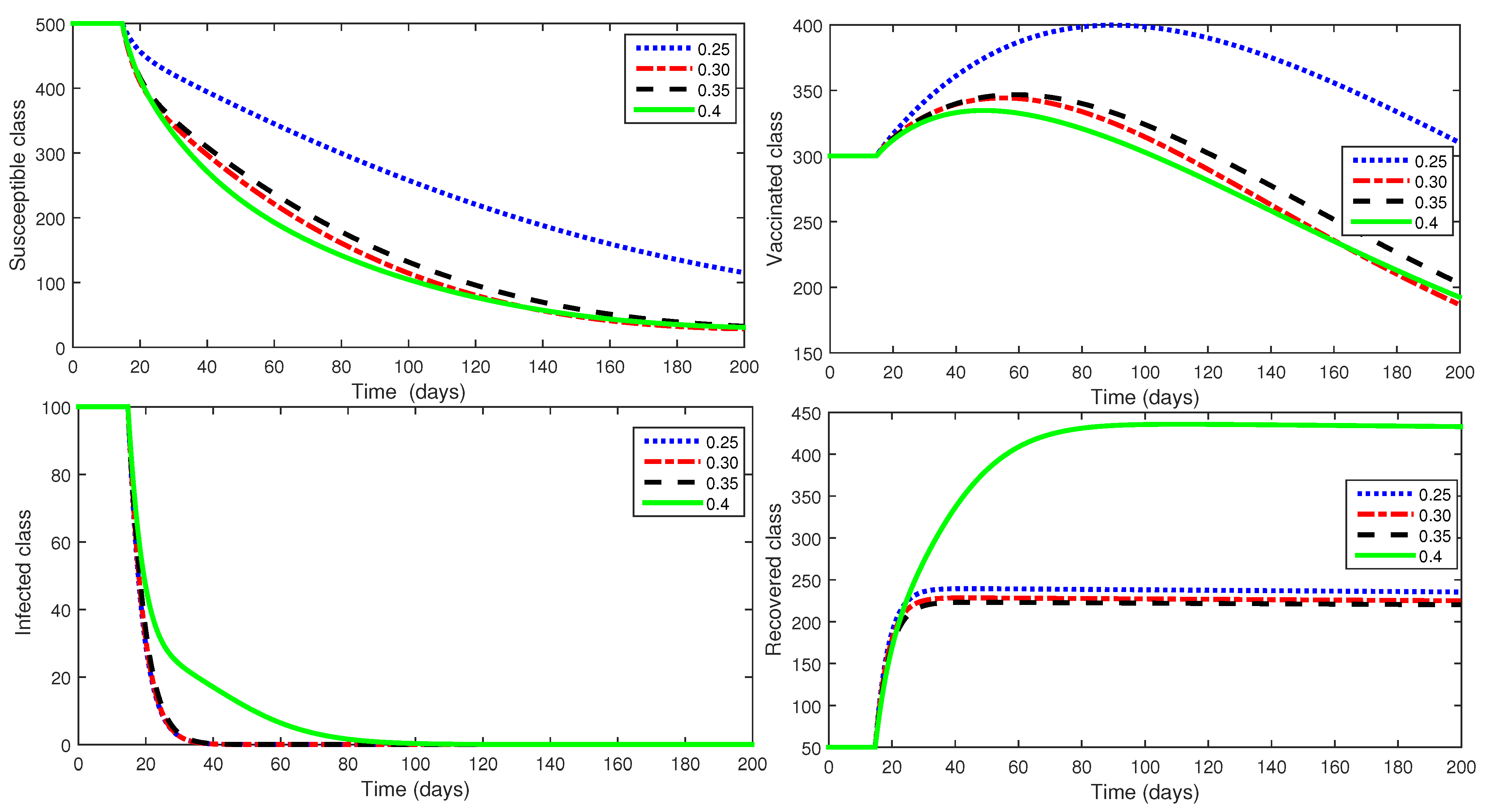
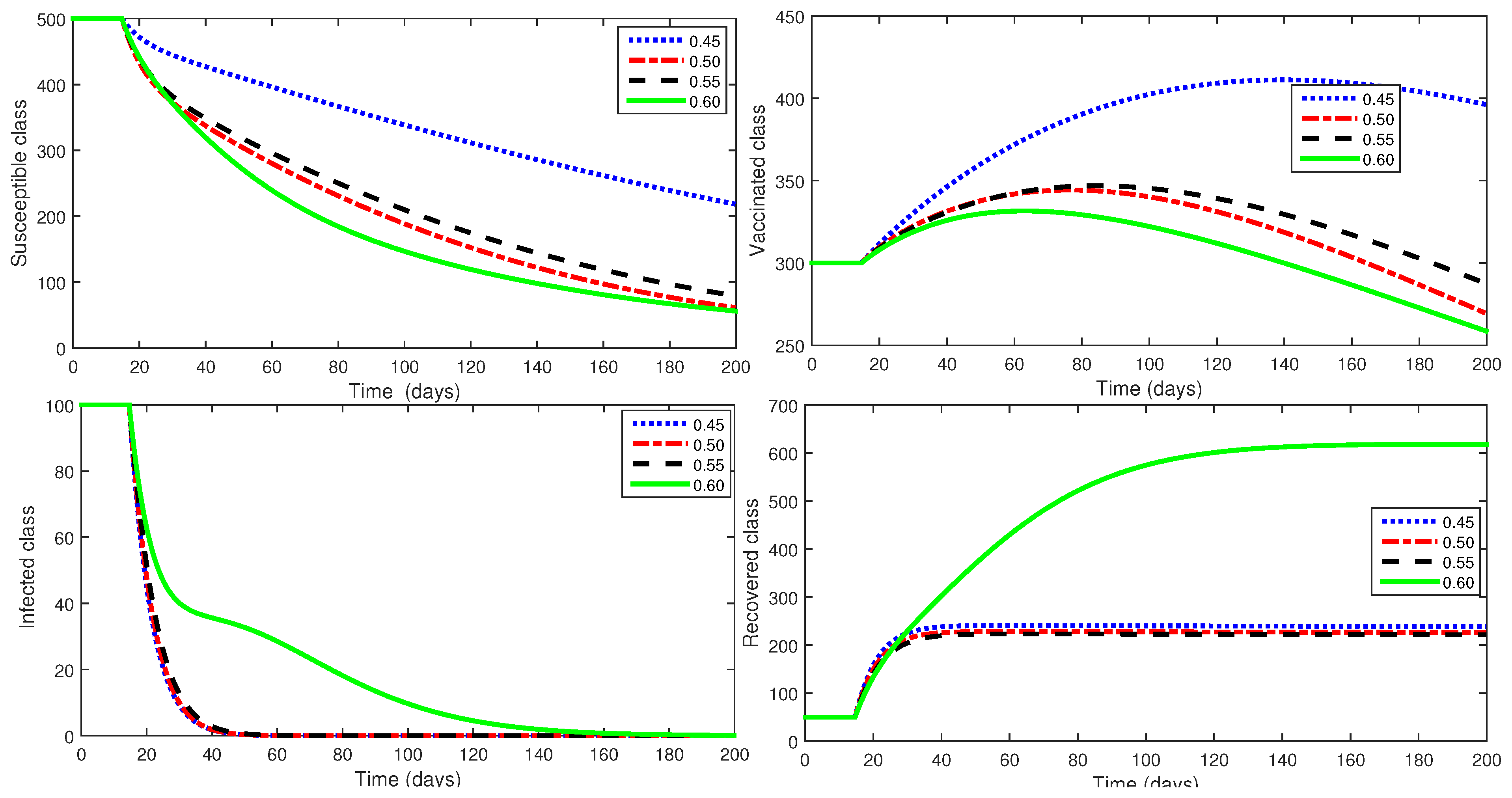
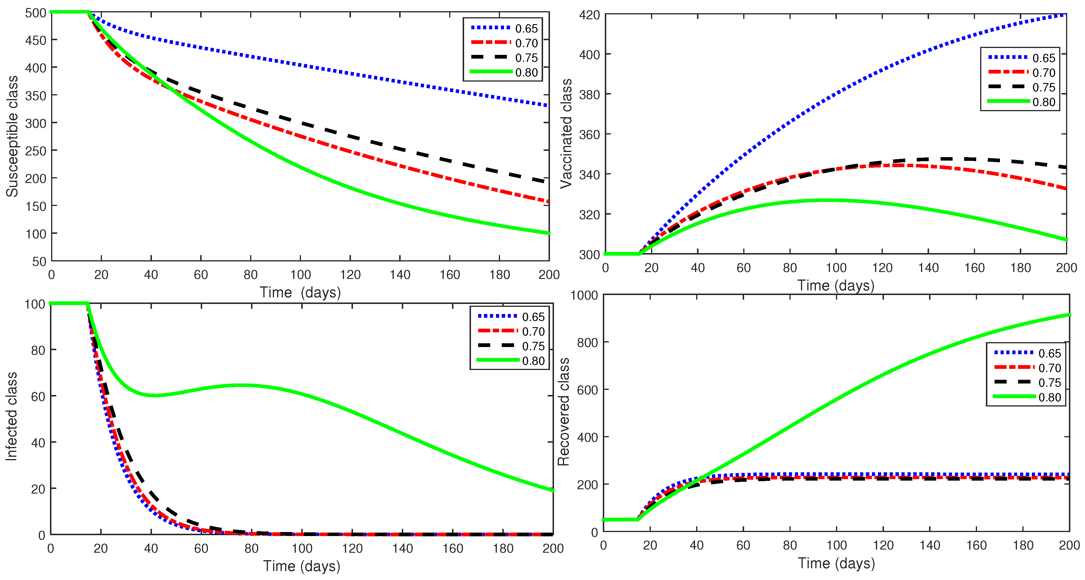
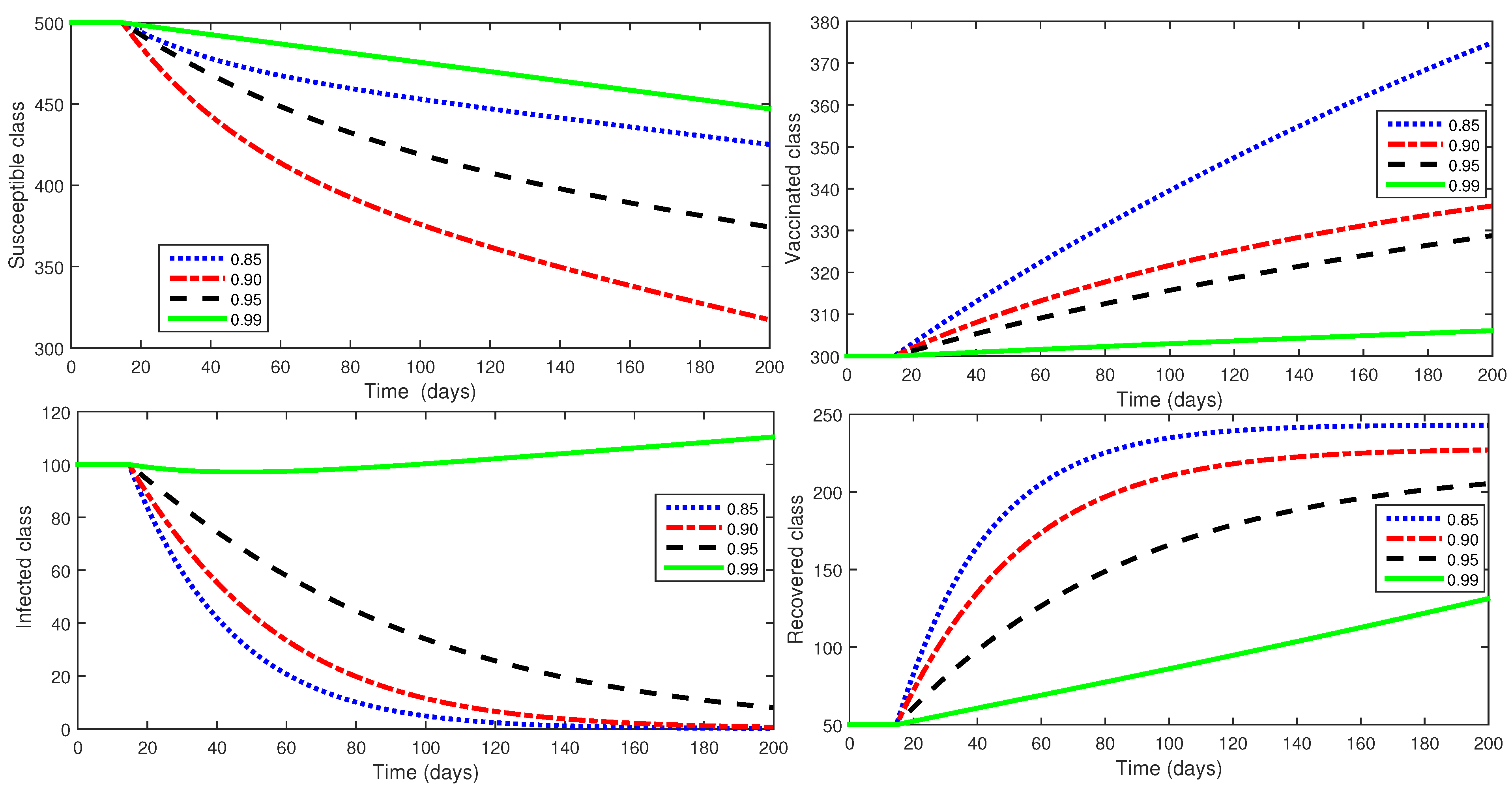
This part presents the numerical simulation employing the resulting method under the ideas of classical and piecewise derivatives, as shown in Figure 6, Figure 7, Figure 8, Figure 9 and Figure 10. The interval is divided into two subintervals. The first interval is checked for an integer order derivative, and the second interval is examined using data from Table 2 on various fractional orders in terms of the Caputo derivative.
In Figure 6, we present the approximate solution to our proposed Model (3) by splitting the domain [ 0 , 200 ] as J 1 = [ 0 , 20 ] , J 2 = ( 20 , 200 ] using the fractional order values in ( 0 , 0.4 ] . Here, T = 200 , t 1 = 20 . We see that as the vaccination process continues increasing, and the infected class shows a decline in its population dynamics. Furthermore, the recovered class increases. The decline is clear from the susceptible class. Due to various fractional order values, the increase and decrease behaviors in various compartments are different. Usually, when a fractional order is smaller, the decay process will be faster and the growth process will be slower. On the other hand, the larger the fractional order, the faster the growth process and the slower the decay process.
In Figure 7, we present the approximate solution to our proposed Model (3) by splitting the domain [ 0 , 200 ] as J 1 = [ 0 , 20 ] , J 2 = ( 20 , 200 ] using the fractional order values in [ 0.45 , 0.60 ] . We see that as the vaccination process goes on increasing, the infected class shows a decline in its population dynamics. Furthermore, the recovered class increases. The decline is clear from the susceptible class.
In Figure 8, we present the approximate solution to our proposed Model (3) by splitting the domain [ 0 , 200 ] as J 1 = [ 0 , 20 ] , J 2 = ( 20 , 200 ] using the fractional order values in [ 0.45 , 0.60 ] . We see that as the vaccination process increases, the infected class shows a decline in its population dynamics. Furthermore, the recovered class increases. The decline is clear in the susceptible class.
With the same process, in Figure 9, we present the approximate solution to our proposed Model (3) using the fractional order values in [ 0.85 , 0.99 ] . We see that as the vaccination process goes on increasing, the infected class shows a decline in its population dynamics. Furthermore, the recovered class increases. The decline is clear in the susceptible class.
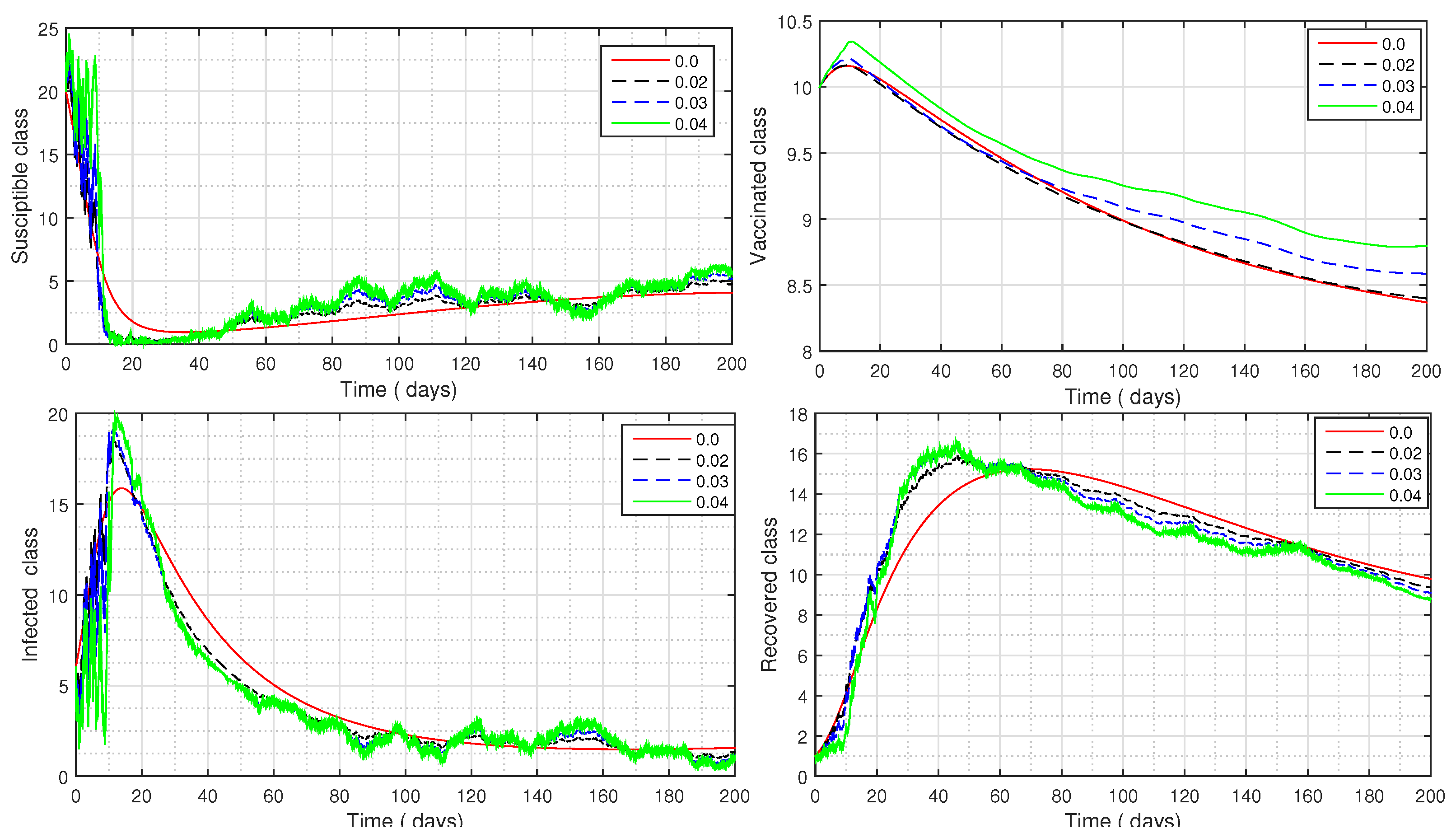
Here, in Figure 10, we present the numerical illustration of Model (3) corresponding to different values of white noise σ i ( i = 1 , 2 , 3 , 4 ) . The concerned variation in the dynamics of a different compartment can be seen in Figure 10.
Due to the exacting mathematical formulation of these connections, a thorough analysis of all dynamic processes involved in disease transmission is required. As a result, creating a mathematical model aids in concentrating thought on the crucial processes that shape the epidemiology of an infectious disease and identifies the parameters that have the most influence and are most amenable to control. Therefore, mathematical modeling is integrative in that it brings together knowledge from widely disparate fields like microbiology, the social sciences, and clinical sciences. Even though rotavirus causes substantial morbidity in both affluent and developing nations, it is also associated with extremely high mortality in the latter. More than 85% of rotavirus-related fatalities are thought to occur in Asia, Latin America, and Africa. Here, we present the said disease model with some new perspectives of fractional calculus. Theoretical results are presented graphically using different fractional orders in Figure 6, Figure 7, Figure 8 and Figure 9. For more sophisticated results, the stochastic version is also presented graphically in Figure 10.

6. Conclusions

Here, a fractional order model in the sense of a piecewise derivative has been investigated in order to examine the complex behavior of the rotavirus infectious disease. Additional analysis is provided, including information on the suggested model’s equilibrium points, fundamental reproduction number, existence, and non-negativity of the solution.The stability effects for local and global scenarios are thoroughly examined. This study has introduced the idea of the piecewise differential and integral operators in a piecewise format. The existence theory of the solution to the suggested model has been demonstrated by the use of Schauder and Banach’s fixed-point theorems. Additionally, a numerical methodology based on the modified Euler technique has been devised. After that, the findings were graphically displayed for a range of fractional orders using some actual data. Furthermore, concerning outcomes have been illustrated and contrasted with actual facts in the instance of persons who have been reported to be infected. Abrupt shifts in their condition of rest or uniform motion, also known as crossover behavior, occur in many real-world scenarios. Conventional derivatives, whether fractional or classical, are unable to adequately illustrate this phenomenon. The phenomenon in question is well-explained using piecewise derivatives of a fractional order. Based on the numerical findings, it can be said that the fractional-order derivative provides more information about the suggested model than the traditional integer-order epidemic models. This kind of research can be applied in the future to more intricate dynamical issues including derivatives of the fractal-fractional and Mittag–Leffler types. Furthermore, employing optimal control procedures and non-singular differential operators, the aforementioned model will be examined under stochastic fractional order differential equations in the future.

Author Contributions

Conceptualization, N.H.A. and M.B.J.; methodology, M.B.J.; software, M.B.J.; validation, N.H.A.; formal analysis, M.B.J.; investigation, M.B.J.; resources, N.H.A.; data curation, N.H.A.; writing—original draft preparation, M.B.J.; writing—review and editing, M.B.J.; visualization, N.H.A.; supervision, N.H.A.; project administration, M.B.J.; funding acquisition, N.H.A. All authors have read and agreed to the published version of the manuscript.

Funding

The authors extend their appreciation to the Deputyship for Research and Innovation, Ministry of Education in Saudi Arabia, for funding this research through project number IFP-IMSIU-2023126. The authors also appreciate the Deanship of Scientific Research at Imam Mohammad Ibn Saud Islamic University (IMSIU) for supporting and supervising this project.

Data Availability Statement

Not applicable.

Acknowledgments

The authors extend their appreciation to the Deputyship for Research and Innovation, Ministry of Education in Saudi Arabia, for funding this research through project number IFP-IMSIU-2023126. The authors also appreciate the Deanship of Scientific Research at Imam Mohammad Ibn Saud Islamic University (IMSIU) for supporting and supervising this project.

Conflicts of Interest

The authors declare no conflict of interest.

References

  1. World Health Organization. Generic Protocol for Monitoring Impact of Rotavirus Vaccination on Gastroenteritis Disease Burdenand Viral Strains; World Health Organization: Geneva, Switzerland, 2008. [Google Scholar]
  2. Ramig, R.F. Pathogenesis of intestinal and systemic rotavirus infection. J. Virol. 2004, 78, 10213–10220. [Google Scholar] [CrossRef]
  3. Muendo, C.; Laving, A.; Kumar, R.; Osano, B.; Egondi, T.; Njuguna, P. Prevalence of rotavirus infection among children with acute diarrhoea after rotavirus vaccine introduction in Kenya, a hospital cross-sectional study. BMC Pediatr. 2018, 18, 1–9. [Google Scholar] [CrossRef]
  4. Anderson, E.J.; Weber, S.G. Rotavirus infection in adults. Lancet Infect. Dis. 2004, 4, 91–99. [Google Scholar] [CrossRef]
  5. Bishop, R.F. Natural history of human rotavirus infection. Viral Gastroenteritis 1996, 119–128. [Google Scholar]
  6. Lambisia, A.W.; Onchaga, S.; Murunga, N.; Lewa, C.S.; Nyanjom, S.G.; Agoti, C.N. Epidemiological trends of five common diarrhea-associated enteric viruses pre-and post-rotavirus vaccine introduction in coastal Kenya. Pathogens 2020, 9, 660. [Google Scholar] [CrossRef]
  7. Shah, K.; Din, R.U.; Deebani, W.; Kumam, P.; Shah, Z. On nonlinear classical and fractional order dynamical system addressing COVID-19. Results Phys. 2021, 24, 104069. [Google Scholar] [CrossRef]
  8. Wang, Y.; Wei, Z.; Cao, J. Epidemic dynamics of influenza-like diseases spreading in complex networks. Nonlinear Dyn. 2020, 101, 1801–1820. [Google Scholar] [CrossRef]
  9. Diekmann, O.; Heesterbeek, J.A.P. Mathematical Epidemiology of Infectious Diseases: Model Building, Analysis and Interpretation; John Wiley & Sons: Hoboken, NJ, USA, 2020; Volume 5. [Google Scholar]
  10. Mondal, J.; Khajanchi, S. Mathematical modeling and optimal intervention strategies of the COVID-19 outbreak. Nonlinear Dyn. 2022, 109, 177–202. [Google Scholar] [CrossRef]
  11. Omondi, O.L.; Wang, C.; Xue, X.; Lawi, O.G. Modeling the effects of vaccination on rotavirus infection. Adv. Differ. Equ. 2015, 2015, 381. [Google Scholar] [CrossRef]
  12. Ilmi, N.B.; Darti, I.; Suryanto, A. Dynamical Analysis of a rotavirus infection model with vaccination and saturation incidence rate. J. Phy. Conf. Ser. 2020, 1562, 012018. [Google Scholar] [CrossRef]
  13. Darti, I.; Suryanto, A.; Ilmi, N.B. Dynamical behavior of a rotavirus transmission model with an environmental effects. In AIP Conference Proceedings; AIP Publishing LLC.: Melville, NY, USA, 2020; p. 020001. [Google Scholar]
  14. Ahmad, S.; Ullah, A.; Arfan, M.; Shah, K. On analysis of the fractional mathematical model of rotavirus epidemic with the effects of breastfeeding and vaccination under atangana-baleanu (ab) derivative. Chaos Solitons Fractals 2020, 140, 110233. [Google Scholar] [CrossRef]
  15. Asare, E.O.; Al-Mamun, M.A.; Armah, G.E.; Lopman, B.A.; Parashar, U.D.; Binka, F.; Pitzer, V.E. Modeling of rotavirus transmission dynamics and impact of vaccination in ghana. Vaccine 2020, 38, 4820–4828. [Google Scholar] [CrossRef]
  16. Asamoah, J.K.K. A fractional mathematical model of heartwater transmission dynamics considering nymph and adult amblyomma ticks. Chaos Solitons Fractals 2023, 174, 113905. [Google Scholar] [CrossRef]
  17. Riewe, F. Mechanics with fractional derivatives. Phys. Rev. E 1997, 55, 3581. [Google Scholar] [CrossRef]
  18. Li, C.; Deng, W. Remarks on fractional derivatives. Appl. Math. Comput. 2007, 187, 777–784. [Google Scholar] [CrossRef]
  19. De Oliveira, E.C.; Tenreiro Machado, J.A. A review of definitions for fractional derivatives and integral. Math. Probl. Eng. 2014, 2014, 238459. [Google Scholar] [CrossRef]
  20. Magin, R. Fractional calculus in bioengineering, part 1. Crit. Rev. Biomed. Eng. 2004, 32, 1–104. [Google Scholar]
  21. Magin, R.L. Fractional calculus in bioengineering: A tool to model complex dynamics. In Proceedings of the 13th International Carpathian Control Conference (ICCC), Podbanske, Slovakia, 28–31 May 2012; pp. 464–469. [Google Scholar]
  22. Magin, R.L. Fractional calculus models of complex dynamics in biological tissues. Comput. Math. Appl. 2010, 59, 1586–1593. [Google Scholar] [CrossRef]
  23. Machado, J.T.; Kiryakova, V.; Mainardi, F. Recent history of fractional calculus. Commun. Nonlinear Sci. Numer. Simul. 2011, 16, 1140–1153. [Google Scholar] [CrossRef]
  24. Gómez-Aguilar, J.F.; Razo-Hernández, R.; Granados-Lieberman, D. A physical interpretation of fractional calculus in observables terms: Analysis of the fractional time constant and the transitory response. Rev. Mex. Física 2014, 60, 32–38. [Google Scholar]
  25. Meral, F.C.; Royston, T.J.; Magin, R. Fractional calculus in viscoelasticity: An experimental study. Commun. Nonlinear Sci. Numer. Simul. 2014, 15, 939–945. [Google Scholar] [CrossRef]
  26. Wu, G.C.; Luo, M.; Huang, L.L.; Banerjee, S. Short memory fractional differential equations for new memristor and neural network design. Nonlinear Dyn. 2020, 100, 3611–3623. [Google Scholar] [CrossRef]
  27. Sang, Y.; Liang, S. Fractional Kirchhoff-Choquard equation involving Schrödinger term and upper critical exponent. J. Geom. Anal. 2022, 32, 5. [Google Scholar] [CrossRef]
  28. Zeb, A.; Atangana, A.; Khan, Z.A.; Djillali, S. A robust study of a piecewise fractional order COVID-19 mathematical model. Alex. Eng. J. 2022, 61, 5649–5665. [Google Scholar] [CrossRef]
  29. Atangana, A.; Araz, S.I. New concept in calculus: Piecewise differential and integral operators. Chaos Solitons Fractals 2021, 145, 110638. [Google Scholar] [CrossRef]
  30. Khalsaraei, M.M. An improvement on the positivity results for 2-stage explicit Runge–Kutta methods. J. Comput. Appl. Math. 2010, 235, 137–143. [Google Scholar] [CrossRef]
  31. Etemad, S.; Tellab, B.; Alzabut, J.; Rezapour, S.; Abbas, M.I. Approximate solutions and Hyers-Ulam stability for a system of the coupled fractional thermostat control model via the generalized differential transform. Adv. Differ. Equations 2021, 2021, 1–25. [Google Scholar] [CrossRef]
  32. Li, R.; Zhong, S.; Swartz, C. An improvement of the Arzela-Ascoli theorem. Topol. Its Appl. 2012, 159, 2058–2061. [Google Scholar] [CrossRef]
  33. Agarwal, R.P.; Arshad, S.; O’Regan, D.; Lupulescu, V. A Schauder fixed point theorem in semilinear spaces and applications. Fixed Point Theory Appl. 2013, 2013, 1–13. [Google Scholar] [CrossRef]
  34. Al Elaiw, A.; Hafeez, F.; Jeelani, M.B.; Awadalla, M.; Abuasbeh, K. Existence and uniqueness results for mixed derivative involving fractional operators. AIMS Math. 2023, 8, 7377–7393. [Google Scholar] [CrossRef]
  35. Jeelani, M.B. Stability and computational analysis of COVID-19 using a higher order galerkin time discretization scheme. Adv. Appl. Stat. 2023, 86, 167–206. [Google Scholar] [CrossRef]
  36. Moumen, A.; Shafqat, R.; Alsinai, A.; Boulares, H.; Cancan, M.; Jeelani, M.B. Analysis of fractional stochastic evolution equations by using Hilfer derivative of finite approximate controllability. AIMS Math. 2023, 8, 16094–16114. [Google Scholar] [CrossRef]
  37. Alharthi, N.H.; Jeelani, M.B. A fractional model of COVID-19 in the frame of environmental transformation with Caputo fractional derivative. Adv. Appl. Stat. 2023, 88, 225–244. [Google Scholar] [CrossRef]
  38. Alnahdi, A.S.; Jeelani, M.B.; Wahash, H.A.; Abdulwasaa, M.A. A Detailed Mathematical Analysis of the Vaccination Model for COVID-19. CMES-Comput. Model. Eng. Sci. 2023, 135, 1315–1343. [Google Scholar] [CrossRef]
  39. Dehingia, K.; Jeelani, M.B.; Das, A. Artificial Intelligence and Machine Learning: A Smart Science Approach for Cancer Control. In Advances in Deep Learning for Medical Image Analysis; CRC Press: Boca Raton, FL, USA, 2022; pp. 87–99. [Google Scholar]
  40. Shaikh, M.B.J. Some Application of Differential Transform Methods to Stiff Differential Equations. Int. J. Appl. Eng. Res. 2019, 14, 877–880. [Google Scholar]
  41. Shah, K.; Abdeljawad, T.; Alrabaiah, H. On coupled system of drug therapy via piecewise equations. Fractals 2022, 30, 2240206. [Google Scholar] [CrossRef]
  42. Banihashemi, S.; Jafari, H.; Babaei, A. A stable collocation approach to solve a neutral delay stochastic differential equation of fractional order. J. Comput. Appl. Math. 2022, 403, 113845. [Google Scholar] [CrossRef]
  43. Jumarie, G. Stochastic differential equations with fractional Brownian motion input. Int. J. Syst. Sci. 1993, 24, 1113–1131. [Google Scholar] [CrossRef]
  44. Shah, K.; Abdeljawad, T. Study of a mathematical model of COVID-19 outbreak using some advanced analysis. Waves Random Complex Media 2022, 1–18. [Google Scholar] [CrossRef]
  45. Platen, E. An introduction to numerical methods for stochastic differential equations. Acta Numer. 1999, 8, 197–246. [Google Scholar] [CrossRef]
  46. Khan, S.; Khan, Z.A.; Alrabaiah, H.; Zeb, S. On using piecewise fractional differential operator to study a dynamical system. Axioms 2023, 12, 292. [Google Scholar] [CrossRef]
  47. Kheyami, A.M.; Cunliffe, N.A.; Hart, C.A. Rotavirus infection in Saudi Arabia. Ann. Saudi Med. 2006, 6, 184–191. [Google Scholar] [CrossRef]
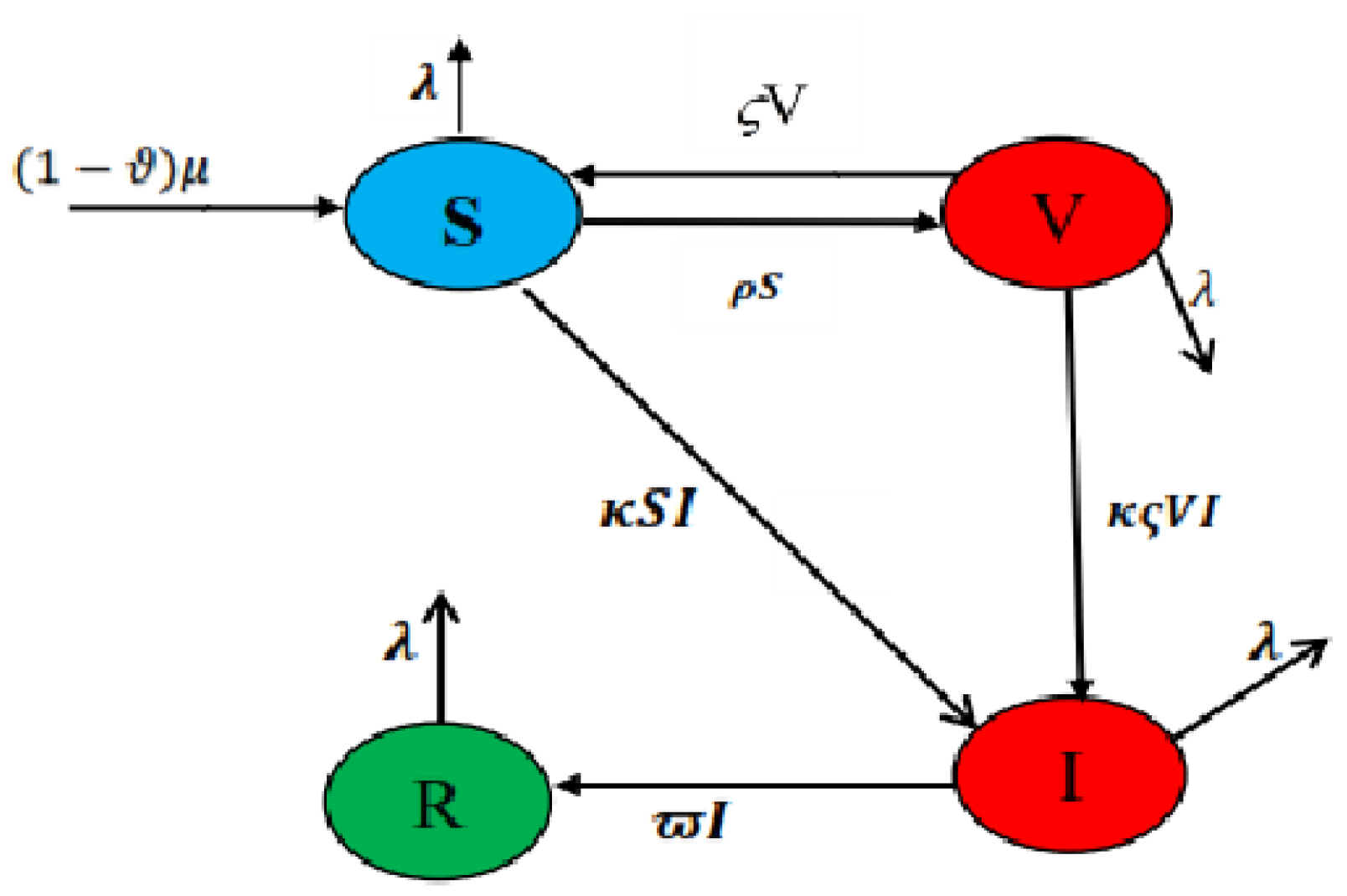
Figure 1. Schematic diagram of our model proposed (3).
Axioms 12 00970 g001
Figure 2. Graphical presentations of reported cases for infected and vaccinated classes of rotavirus in Saudi Arabia.
Axioms 12 00970 g002
Figure 3. A 3D profile of R 0 for the proposed Model (3).
Axioms 12 00970 g003
Figure 4. Presentation of sensitivity index.
Axioms 12 00970 g004
Figure 5. Solution curves of Model (3) at the endemic equilibrium using S 0 = 500 , V 0 = 300 , I 0 = 100 , R 0 = 50 .
Axioms 12 00970 g005
Figure 6. Fractional order dynamics of the proposed Model (3) using fractional orders in ( 0 , 0.4 ] .
Axioms 12 00970 g006
Figure 7. Fractional order dynamics of the proposed Model (3) using fractional orders in [ 0.45 , 0.60 ] .
Axioms 12 00970 g007
Figure 8. Fractional order dynamics of the proposed Model (3) using fractional orders in [ 0.65 , 0.80 ] .
Axioms 12 00970 g008
Figure 9. Fractional order dynamics of the proposed Model (3) using fractional orders in [ 0.65 , 0.80 ] .
Axioms 12 00970 g009
Figure 10. Presentation of stochastic form of the proposed Model (3) using different values of white noise σ i ( i = 1 , 2 , 3 , 4 ) .
Axioms 12 00970 g010
Table 1. Sensitivity of the R 0 versus proposed parameters.
ParameterSensitivity IndexValueParameterSensitivity IndexValue
μ S μ R 0 1 τ S τ R 0 −0.0004507
κ S κ R 0 1 ω S ω R 0 −0.00025608
λ S λ R 0 −1.0002560
Table 2. Description and specification of real values for the variables used in the system (2).
ParametersNumerical Value
S500 [28]
V300 [28]
I100 [28]
R50 [28]
μ 0.4109 [28]
ϑ 0.001884 [28]
λ 0.00002537 [28]
τ 0.00004466 [28]
κ 0.0001 [28]
ω 0.099 [28]
ζ 0.001 [28]
ς 0.001884 [28]
ρ 0.002778 [28]
Disclaimer/Publisher’s Note: The statements, opinions and data contained in all publications are solely those of the individual author(s) and contributor(s) and not of MDPI and/or the editor(s). MDPI and/or the editor(s) disclaim responsibility for any injury to people or property resulting from any ideas, methods, instructions or products referred to in the content.