On the Timelike Circular Surface and Singularities in Minkowski 3-Space

Abstract

In this paper, we have parameterized a timelike ($\mathcal{T}like$) circular surface ($\mathcal{CI}\mathit{surface}$) and have obtained its geometric properties, including striction curves, singularities, Gaussian and mean curvatures. Afterward, the situation for a $\mathcal{T}like$ roller coaster surface ($\mathcal{RCO}\mathit{surface}$) to be a flat or minimal surface is examined in detail. Further, we illustrate the approach’s outcomes with a number of pertinent examples.

1. Introduction

One of the essential goals of the vintage differential geometry is the debate on some categories of surfaces with specific properties in both Minkowski 3-space ${\mathbb{E}}_1^3$ and Euclidean 3-space ${\mathbb{E}}^3$ such as ruled and developable surfaces, minimal surfaces, etc. [1,2,3,4,5,6,7,8,9,10]. A ruled surface is a type of surface that is generated by a moving line that travels along a given curve. The distinct attitudes of the designing lines are the rulings of the surface. Developable surfaces are a specific type of ruled surface, characterized by the property that all points lying on the same generating line share the same tangent plane. It is worth noting that the Gaussian curvature vanishes everywhere on the surface, and the generating lines can be viewed as curvature lines exhibiting the vanishing normal curvature. Hence, the application of ruled surfaces in various fields, including product design, manufacturing, locomotion analysis, imitation of rigid bodies, and model-based target admission frameworks, has been extensive. There is a substantial body of literature available on the subject, which includes various monographs (see, e.g., [11,12,13]).

A canonical $\mathcal{CI}\mathit{surface}$ is a subset of surfaces that are relatively easier to systematically and kinematically characterize. There exist two distinct categories of canonical $\mathcal{CI}\mathit{surfaces}$ (see, e.g., [14,15,16,17,18,19,20]). The first surface is referred to as the canonical $\mathcal{CI}\mathit{surface}$, whereas the second surface is known as the non-canonical $\mathcal{CI}\mathit{surface}$. The cross-section of a canonical $\mathcal{CI}\mathit{surface}$ is a circle, and the normal of the circle plane is largely symmetrical to the cross-section. Previous work has discussed other classes of the canonical $\mathcal{CI}\mathit{surface}$, including the tubular surface, pipe surface, string, and canal surface. These classes exhibit comparative diversity. Occasionally, certain books on differential geometry have made a distinction by referring to them as offset surfaces. The term “canonical $\mathcal{CI}\mathit{surface}$” refers to the surface that encompasses a collection of circles with variable radii [16]. A non-canonical $\mathcal{CI}\mathit{surface}$ is characterized by having a non-circular cross-section and a circle plane with a normal vector that is notably not parallel to the normal vector of the cross-section.

There is an adjacent organization within ruled surfaces and $\mathcal{CI}\mathit{surfaces}$. The characteristics of a tangential ruled surface are straight lines, which are tangential to the limit of regression. The limit of regression interprets the singular points of the tangential developable surface. Izumiya et al. [17] utilized the technique of mobile frames to inspect the $\mathcal{CI}\mathit{surfaces}$ with steady radii. They focused on several symmetrical characteristics of $\mathcal{CI}\mathit{surfaces}$ with ruled surfaces, and reconnoitred the singularities of $\mathcal{CI}\mathit{surfaces}$. In the Minkowski 3-space ${\mathbb{E}}_1^3$, the Lorentzian metric possesses three possible Lorentzian causal characteristics, namely positive, negative, or zero. In contrast, the metric in Euclidean 3-space ${\mathbb{E}}^3$, can only be positive definite. Hence, the kinematic and geometric aspects can yield additional significance in the context of ${\mathbb{E}}_1^3$ [3,4,5].

The current study encompasses the following parts: In Section 2, we sum up the applicable definitions and consequences on curves and surfaces in Minkowski 3-space ${\mathbb{E}}_1^3$. In Section 3, we explain and research geometrical characteristics and singularities of $\mathcal{T}like$ $\mathcal{CI}\mathit{surfaces}$ with steady radii via those of ruled surfaces. Then we extend the characteristics of $\mathcal{T}like$ $\mathcal{CI}\mathit{surfaces}$ to a certain sort of $\mathcal{T}like$ $\mathcal{CI}\mathit{surfaces}$ coined $\mathcal{T}like$ $\mathcal{RCO}\mathit{surface}$. Meanwhile, we designed new epitomes with figures supporting our idea of how to organize $\mathcal{T}like$ $\mathcal{RCO}\mathit{surfaces}$ and $\mathcal{T}like$ $\mathcal{CI}\mathit{surfaces}$.

2. Basic Concepts

This section provides a concise overview of the theory of curves and surfaces in Minkowski 3-space ${\mathbb{E}}_1^3$ [3,4,5]. Let ${\mathbb{E}}_1^3$ denote the Minkowski 3-space. For any $\mathit{\psi }=\left({\psi }_1,{\psi }_2,{\psi }_3\right)$ $\in {\mathbb{E}}_1^3$ the Lorentzian metric $<,>$ can be represented by

$$<\mathit{\psi },\mathit{\psi }>={\psi }_1^2+{\psi }_2^2-{\psi }_3^2.$$

Considering that $<,>$ is not positive definite, it follows that there are three distinct types of vectors in ${\mathbb{E}}_1^3$. A vector $\mathit{\psi }\in {\mathbb{E}}_1^3$ is a spacelike ($\mathcal{S}like$) if $<\mathit{\psi },\mathit{\psi }>>0$ or $\mathit{\psi }=\mathbf{0}$, a $\mathcal{T}like$ if $<\mathit{\psi },\mathit{\psi }><0$, and a lightlike ($\mathcal{L}like$) or null if $<\mathit{\psi },\mathit{\psi }>=0$ and $\psi \ne \mathbf{0}$. Likewise, a regular curve in ${\mathbb{E}}_1^3$ can be $\mathcal{S}like$, $\mathcal{T}like$, or null ($\mathcal{L}like$), if all of its tangent vectors are $\mathcal{S}like$, $\mathcal{T}like$, or null ($\mathcal{L}like$), respectively. For any two vectors $\mathit{\psi }=\left({\psi }_1,{\psi }_2,{\psi }_3\right)$ and $\mathit{\omega }=({\omega }_1,{\omega }_2,{\omega }_3)$ of ${\mathbb{E}}_1^3$, the vector product is

$$\mathit{\psi }\times \mathit{\omega }=\left|\begin{array}{ccc}{\mathit{ϵ}}_1& {\mathit{ϵ}}_2& -{\mathit{ϵ}}_3\\ {\psi }_1& {\psi }_2& {\psi }_3\\ {\omega }_1& {\omega }_2& {\omega }_3\end{array}\right|=\left(-({\omega }_2{\psi }_3-{\omega }_3{\psi }_2),({\omega }_3{\psi }_1-{\omega }_1{\psi }_3),-({\omega }_1{\psi }_2-{\omega }_2{\psi }_1)\right),$$

where ${\mathit{ϵ}}_1$, ${\mathit{ϵ}}_2$, ${\mathit{ϵ}}_3$ is the canonical basis of ${\mathbb{E}}_1^3$. For $\mathit{\psi }\in {\mathbb{E}}_1^3$, the norm is specified by $∥\mathit{\psi }∥=\sqrt{\left|<\mathit{\psi },\mathit{\psi }>\right|}$, and the Lorentzian and hyperbolic unit spheres are, respectively,

$${\mathbb{S}}_1^2=\{\mathit{\psi }\in {\mathbb{E}}_1^3\mid {∥\mathit{\psi }∥}^2={\psi }_1^2+{\psi }_2^2-{\psi }_3^2=1\},$$

and

$${\mathbb{H}}_{+}^2=\{\mathit{\psi }\in {\mathbb{E}}_1^3\mid {∥\mathit{\psi }∥}^2={\psi }_1^2+{\psi }_2^2-{\psi }_3^2=-1,{\psi }_3\ge 1\}.$$

The surface M in ${\mathbb{E}}_1^3$ is denoted by

$$M:\mathbf{q}(v,\mu )=\left(q_1\left(v,\mu \right),q_2\left(v,\mu \right),q_3(\left(v,\mu \right)\right),(v,\mu )\in \mathbb{D}\subseteq {\mathbb{R}}^2.$$

(1)

The unit vector normal is $\zeta (v,\mu )={\mathbf{q}}_v\times {\mathbf{q}}_{\mu }{∥{\mathbf{q}}_v\times {\mathbf{q}}_{\mu }∥}^{-1}$, where ${\mathbf{q}}_i=\frac{\partial \mathbf{q}}{\partial i}$. The first fundamental form I is represented by

$$I=l_{11}d{v}^2+2l_{12}dvd\mu +l_{22}d{\mu }^2,$$

where $l_{11}=<{\mathbf{q}}_v,{\mathbf{q}}_v>$, $l_{12}=<{\mathbf{q}}_v,{\mathbf{q}}_{\mu }>,l_{22}=<{\mathbf{q}}_{\mu },{\mathbf{q}}_{\mu }>$. The 2nd fundamental form $II$ is pointed by

$$II=m_{11}d{v}^2+2m_{12}dvd\mu +m_{22}d{\mu }^2,$$

where $m_{11}=<{\mathbf{q}}_{vv},\mathit{\zeta }>$, $m_{12}=<{\mathbf{q}}_{v\mu },\mathit{\zeta }>,m_{22}=<{\mathbf{q}}_{\mu \mu },\mathit{\zeta }>$. The Gaussian curvature K and the mean curvature H, respectively, are

$$K(v,\mu )=ϵ\frac{m_{11}{m}_{22}-m_{12}^2}{l_{11}{l}_{22}-l_{12}^2},H(v,\mu )=\frac{m_{11}{l}_{11}-2m_{12}{l}_{12}+m_{22}{l}_{22}}{2(l_{11}{l}_{22}-l_{12}^2)},$$

(2)

where $<\mathit{\zeta },\mathit{\zeta }>=\mathit{ϵ}(\pm 1)$.

Definition 1. 

M in ${\mathbb{E}}_1^3$ is a $\mathcal{T}like$ ($\mathcal{S}like$) surface if its normal vector is a $\mathcal{S}like$ ($\mathcal{T}like$) vector [14,15].

3. Timelike Circular Surfaces

This section focuses on the characterization of $\mathcal{T}like$ $\mathcal{CI}\mathit{surfaces}$. Assume a non-null curve $\mathit{\gamma }\left(v\right)$, that is, a curve with ${\mathit{\gamma }}^{\prime }\left(v\right)$ such that $∥{\mathit{\gamma }}^{\prime }\left(v\right)∥\ne 0$ for every $v\in \mathbb{R}$, and a positive number $r>0$. Then a $\mathcal{T}like$ $\mathcal{CI}\mathit{surface}$ can be defined as the surface that is generated by a one-parameter family of Lorentzian circles, where the centers of these circles lie on the given curve $\mathit{\gamma }({}^{\prime }\stackrel{def}{=}\frac{d}{dv})$. Each Lorentzian circle can be described as a creating (generating) circle that lies on a plane referred to as the circle plane. Let $\mathit{\chi }$ symbolize the $\mathcal{S}like$ unit normal vector of a Lorentzian circle plane and $\mathit{\chi }$ be linked with any point of the spine curve $\mathit{\gamma }$, given radii r of the created Lorentzian circle; a $\mathcal{T}like$ $\mathcal{CI}\mathit{surface}$ is represented by both $\mathit{\gamma }$ and $\mathit{\chi }$. The spherical image of $\mathit{\chi }$ is a $\mathcal{T}like$ or $\mathcal{S}like$ curve on a Lorentzian unit sphere, that is, $\mathit{\chi }:I\to {\mathbb{S}}_1^2\subseteq {\mathbb{E}}_1^3$. In this work, we will study the $\mathcal{T}like$ $\mathcal{CI}\mathit{surfaces}$ with the non-null spine curve $\mathit{\gamma }$, and the spherical image of $\mathit{\chi }$ is a $\mathcal{S}like$ curve of class $C^k$ with k sufficiently large.

If v is the arc length of the spherical image of $\mathit{\chi }\in {\mathbb{S}}_1^2$, then the Blaschke frame is

$$\begin{array}{c}{\mathit{\chi }}_1=\mathit{\chi }\left(v\right),{\mathit{\chi }}_2\left(v\right)={\mathit{\chi }}^{\prime }\left(v\right){∥{\mathit{\chi }}^{\prime }\left(v\right)∥}^{-1},{\mathit{\chi }}_3\left(v\right)={\mathit{\chi }}_1\times {\mathit{\chi }}_2,\\ <{\mathit{\chi }}_1,{\mathit{\chi }}_1>=<{\mathit{\chi }}_2,{\mathit{\chi }}_2>=-<{\mathit{\chi }}_3,{\mathit{\chi }}_3>=1,\\ {\mathit{\chi }}_1\times {\mathit{\chi }}_2={\mathit{\chi }}_3,{\mathit{\chi }}_1\times {\mathit{\chi }}_3={\mathit{\chi }}_2,{\mathit{\chi }}_2\times {\mathit{\chi }}_3=-{\mathit{\chi }}_1.\end{array}$$

(3)

Then, the Blaschke formulae are

$$\left(\begin{array}{c}{\mathit{\chi }}_1^{\prime }\hfill \\ {\mathit{\chi }}_2^{\prime }\hfill \\ {\mathit{\chi }}_3^{\prime }\hfill \end{array}\right)=\left(\begin{array}{ccc}0\hfill & 1\hfill & 0\hfill \\ -1\hfill & 0\hfill & \alpha \left(v\right)\hfill \\ 0\hfill & \alpha \left(v\right)\hfill & 0\hfill \end{array}\right)\left(\begin{array}{c}{\mathit{\chi }}_1\hfill \\ {\mathit{\chi }}_2\hfill \\ {\mathit{\chi }}_3\hfill \end{array}\right),$$

(4)

where $\alpha \left(v\right)$ is the spherical (geodesic) curvature function of $\mathit{\chi }\left(v\right)\in {\mathbb{S}}_1^2$. Further, ${\mathit{\chi }}_2$ and ${\mathit{\chi }}_3$ form a basis of the Lorentzian circle plane at each point of $\mathit{\gamma }$. The tangent vector of $\mathit{\gamma }$ is

$${\mathit{\gamma }}^{\prime }\left(v\right)=\delta \left(v\right){\mathit{\chi }}_1\left(v\right)+\sigma \left(u\right){\mathit{\chi }}_2\left(v\right)+\eta \left(v\right){\mathit{\chi }}_3\left(v\right),$$

(5)

where $\delta \left(v\right)$, $\sigma \left(v\right)$, and $\eta \left(v\right)$ are the curvature functions (invariants) of $\mathit{\gamma }\left(v\right)$. Therefore, for a positive value of r, and according to the differential system Equation (4), it is possible to obtain a $\mathcal{T}like$ $\mathcal{CI}\mathit{surface}$ M as follows:

$$M:\mathbf{q}(v,\mu )=\mathit{\gamma }\left(v\right)+r\left(sinh\mu {\mathit{\chi }}_2\left(v\right)+cosh\mu {\mathit{\chi }}_3\left(v\right)\right),(v,\mu )\in \mathbb{D}\subseteq {\mathbb{R}}^2$$

(6)

where $\mu \to$$\mathit{\gamma }$$\left(v\right)+r\left(sinh\mu {\mathit{\chi }}_2\left(v\right)+cosh\mu {\mathit{\chi }}_3\left(v\right)\right)$ creates the Lorentzian circle [15,16,17]. It is evident that Equation (6) assigns a technique for constructing $\mathcal{T}like$ $\mathcal{CI}\mathit{surfaces}$ with a specified radii $r>0$ as

$$\mathit{\gamma }\left(v\right)={\mathit{\gamma }}_0+(\int \delta \left(v\right){\mathit{\chi }}_1\left(v\right)+\sigma \left(v\right){\mathit{\chi }}_2\left(v\right)+\eta \left(v\right){\mathit{\chi }}_3\left(v\right))dv,$$

(7)

where ${\mathit{\gamma }}_0$ is a steady vector. The invariants $\delta \left(v\right)$, $\sigma \left(v\right)$, $\eta \left(v\right)$, and $\alpha \left(v\right)$ allow the geometric advantages of M with $r>0$. In this work, we remove $\mathcal{T}like$ $\mathcal{CI}\mathit{surfaces}$ with ${\mathit{\chi }}_1$ being a constant vector, whose geometrical ownerships are of little benefit.

Through rigorous computational analysis, we obtain

$$\left.\begin{array}{c}{\mathbf{q}}_{\mu }(v,\mu )=r(cosh\mu {\mathit{\chi }}_2+sinh\mu {\mathit{\chi }}_3),\\ {\mathbf{q}}_v(v,\mu )=(\delta -r\alpha sinh\mu ){\mathit{\chi }}_1+(\sigma +r\alpha cosh\mu ){\mathit{\chi }}_2+(\eta +r\alpha sinh\mu ){\mathit{\chi }}_3.\end{array}\right\}$$

(8)

Then,

$$\begin{array}{c}{l}_{11}=<{\mathbf{q}}_v,{\mathbf{q}}_v>={(\delta -rsinh\mu )}^2+{(\sigma +\alpha rcosh\mu )}^2-{(\eta +\alpha rsinh\mu )}^2,\\ l_{12}=<{\mathbf{q}}_v,{\mathbf{q}}_{\mu }>=r(r\alpha +\sigma cosh\mu -\eta sinh\mu ),l_{22}=<{\mathbf{q}}_{\mu },{\mathbf{q}}_{\mu }>=r^2.\end{array}$$

(9)

The $\mathcal{S}like$ unit vector is

$$\zeta (v,\mu )=\frac{r(\eta sinh\mu -\sigma cosh\mu ){\mathit{\chi }}_1+r(\delta -rsinh\mu )\left(sinh\mu {\mathit{\chi }}_2+cosh\mu {\mathit{\chi }}_3\right)}{∥{\mathbf{q}}_v\times {\mathbf{q}}_{\mu }∥},$$

(10)

where

$$∥{\mathbf{q}}_v\times {\mathbf{q}}_{\mu }∥=r\sqrt{{(\eta sinh\mu -\sigma cosh\mu )}^2-{(\delta -rsinh\mu )}^2}.$$

(11)

Further, we have

$$\begin{array}{c}{\mathbf{q}}_{\mu \mu }(v,\mu )=r(sinh\mu {\mathit{\chi }}_2+cosh\mu {\mathit{\chi }}_3),\\ {\mathbf{q}}_{\mu v}(v,\mu )=-rcosh\mu {\mathit{\chi }}_1+r\alpha \left(sinh\mu {\mathit{\chi }}_2+cosh\mu {\mathit{\chi }}_3\right),\\ {\mathbf{q}}_{vv}(v,\mu )=({\delta }^{\prime }-\sigma ){\mathit{\chi }}_1+(\delta +{\sigma }^{\prime }+\eta \alpha +rsinh\mu ){\mathit{\chi }}_2\\ +(\sigma \alpha +{\eta }^{\prime }){\mathit{\chi }}_3+{\alpha }^{\prime }{\mathbf{q}}_{\mu }+\alpha {\mathbf{q}}_{\mu v}.\end{array}$$

(12)

Then,

$$\begin{array}{ccc}\hfill m_{11}& =& \frac{1}{\sqrt{{(\eta sinh\mu -\sigma cosh\mu )}^2-{(\delta -rsinh\mu )}^2}}\hfill \\ & & \times [r(\delta -rsinh\mu )[r\alpha -({\eta }^{\prime }+\sigma \alpha )sinh\mu -(\delta +rcosh\mu +{\sigma }^{\prime })cosh\mu ],\hfill \\ \hfill m_{12}& =& \frac{r\left[(\eta sinh\mu -\sigma cosh\mu )cosh\mu -\alpha (\delta +rcosh\mu )\right]}{\sqrt{{(\eta sinh\mu -\sigma cosh\mu )}^2-{(rsinh\mu +\delta )}^2}},\hfill \\ \hfill m_{22}& =& -\frac{r\left(\delta +rcosh\mu \right)}{\sqrt{{(\eta sinh\mu -\sigma cosh\mu )}^2-{(rsinh\mu +\delta )}^2}}.\hfill \end{array}$$

(13)

The Gaussian and mean curvatures can be acquired, respectively, as

$$\begin{array}{ccc}\hfill K(v,\mu )& =& \frac{1}{\sqrt{{(\eta sinh\mu -\sigma cosh\mu )}^2-{(rsinh\mu +\delta )}^2}}\{[rsinh\mu (\sigma sinh\mu -\eta cosh\mu )]\hfill \\ & & \times [sinh\mu (\eta sinh\mu -\sigma cosh\mu )+\alpha (rsinh\mu +\delta \left)\right]\hfill \\ & & -(\delta -rsinh\mu )\times [({\delta }^{\prime }-\sigma )(\eta sinh\mu -\sigma cosh\mu )\hfill \\ & & +(\delta -rsinh\mu )(\delta sinh\mu +r{sinh}^2\mu \hfill \\ & & +{\eta }^{\prime }sinh\mu -{\sigma }^{\prime }cosh\mu +\alpha (\sigma \eta sinh\mu -\sigma cosh\mu )\left)\right]\},\hfill \end{array}$$

(14)

and

$$\begin{array}{ccc}\hfill H(v,\mu )& =& \frac{1}{2r{\left[{(\eta sinh\mu -\sigma cosh\mu )}^2-{(\delta -rsinh\mu )}^2\right]}^{3/2}}\{r(\eta sinh\mu -\sigma cosh\mu )\hfill \\ & & \times [{\sigma }^{\prime }+\sigma +\alpha r(cosh\mu -sinh\mu )+2(\eta sinh\mu -\sigma cosh\mu )+\alpha \sigma ]\hfill \\ & & -(\delta -rsinh\mu )\left[\right(\delta -rsinh\mu \left)\right(2rsinh\mu +\sigma )\hfill \\ & & +r({\eta }^{\prime }sinh\mu -{\sigma }^{\prime }cosh\mu )+r({\sigma }^2-{\eta }^2)\}.\hfill \end{array}$$

(15)

Definition 2. 

For a $\mathcal{T}like$ $\mathcal{CI}\mathit{surface}$ M, we have the following:

(1) M is a $\mathcal{T}like$ canal (tubular) surface if γ is perpendicular to the Lorentzian circular plane, that is, χ${}_1\left(v\right),$χ${}_2\left(v\right)$, χ${}_3\left(v\right)$, and ${\mathit{\gamma }}^{\prime }\left(v\right)$ satisfy

$$\delta \left(v\right)=<{\mathit{\chi }}_1,{\mathit{\gamma }}^{\prime }>\ne 0,and<{\mathit{\chi }}_2,{\mathit{\gamma }}^{\prime }>=<{\mathit{\chi }}_3,{\mathit{\gamma }}^{\prime }>=0\iff \sigma \left(v\right)=\eta \left(v\right)=0.$$

(16)

(2) M is a non-canal ($\mathcal{T}like$ $\mathcal{RCO}$) $\mathcal{T}like$ $\mathcal{CI}\mathit{surface}$ if γ is tangent to the Lorentzian circular plane, that is, χ${}_1\left(v\right),$χ${}_2\left(v\right)$, χ${}_3\left(v\right)$, and ${\mathit{\gamma }}^{\prime }\left(v\right)$ satisfy

$$\delta \left(v\right)=<{\mathit{\chi }}_1,{\mathit{\gamma }}^{\prime }>=0,and\sigma \left(v\right)=<{\mathit{\chi }}_2,{\mathit{\gamma }}^{\prime }>=0or\eta \left(v\right)=<{\mathit{\chi }}_3,{\mathit{\gamma }}^{\prime }>=0.$$

(17)

Therefore, the Lorentzian sphere, the $\mathcal{T}like$ canal surface, and the $\mathcal{T}like$ $\mathcal{RCO}\mathit{surface}$ correspond to the cone, the cylinder surface, and the tangent developable surface, respectively. Hence, it is imperative to conduct a comprehensive investigation into the characteristics of $\mathcal{T}like$ $\mathcal{CI}\mathit{surfaces}$, particularly in relation to their similarities to ruled surfaces.

Example 1. 

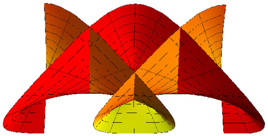
In the next discussion, we will postulate the $\mathcal{T}like$ canal surface for which the parametric curves are principal lines. Since $\sigma \left(v\right)=\eta \left(v\right)=0$, from Equations (9) and (13) it follows that $l_{12}=m_{12}=0\iff \alpha =0$. If we substitute this into Equation (4), we obtain the ODE ${\mathit{\chi }}_1^{″}+{\mathit{\chi }}_1=\mathbf{0}$. The $\mathcal{S}like$ curve that satisfies this ODE is a great circle on ${\mathbb{S}}_1^2$. For example, a $\mathcal{S}like$ great circle can be represented as ${\mathit{\chi }}_1\left(v\right)=(sinv,cosv,0)$. The normal vector can be given from ${\mathit{\chi }}_2={\mathit{\chi }}_1^{\prime }$ as ${\mathit{\chi }}_2\left(v\right)=(cosv,-sinv,0)$. Thus ${\mathit{\chi }}_3\left(v\right)=(0,0,1)$. In this case, via Equation (7), $\mathit{\gamma }\left(v\right)$ can be specified by

$$\mathit{\gamma }\left(v\right)={\mathit{\gamma }}_0+\int \delta \left(v\right)(sinv,cosv,0)dv,$$

where ${\mathit{\gamma }}_0$ is a fixed point. Then, the $\mathcal{T}like$ canal surface pencil is

$$\mathbf{q}(v,\mu )={\mathit{\gamma }}_0+\left(\begin{array}{c}\int \delta \left(v\right)sinvdv+rsinh\mu cosv\\ \int \delta \left(v\right)cosvdv-rsinh\mu sinv\\ rcosh\mu \end{array}\right).$$

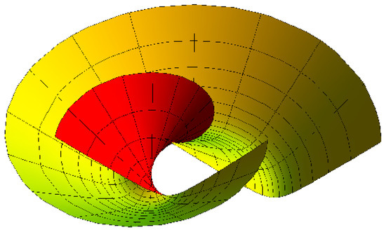
With ${\mathit{\gamma }}_0=\mathbf{0}$, Figure 1 and Figure 2 show members in the pencil with $\delta \left(v\right)=sinv$, v and $r=1$.

Figure 1. $\mathcal{T}like$ canal surface with $r=1$, and $\delta =sinv$.

Figure 2. $\mathcal{T}like$ canal surface with $r=1$, and $\delta =v$.

3.1. Striction Curve

The striction curve of a ruled surface is significant for studying the singularities. Then, we expound a parallel idea for a $\mathcal{T}like$ $\mathcal{CI}\mathit{surface}$ as follows. The curve

$$\mathbf{x}\left(v\right)=\mathit{\gamma }\left(v\right)+r\left(cosh\mu \left(v\right){\mathit{\chi }}_2\left(v\right)+sinh\mu \left(v\right){\mathit{\chi }}_3\left(v\right)\right),$$

is a striction curve on M if and only if

$$<{\mathit{\gamma }}^{\prime },cosh\mu \left(v\right){\mathit{\chi }}_2\left(v\right)+sinh\mu \left(v\right){\mathit{\chi }}_3\left(v\right)>=0.$$

(18)

From Equations (5) and (18), it follows that

$$\sigma \left(v\right)cosh\mu \left(v\right)-\eta \left(v\right)sinh\mu \left(v\right)=0.$$

(19)

From Equation (19), it can be found that

$$sinh\mu \left(v\right)=\frac{\sigma \left(v\right)}{\sqrt{{\eta }^2-{\sigma }^2}},\mathrm{and}cosh\mu \left(v\right)=\frac{\eta \left(v\right)}{\sqrt{{\eta }^2-{\sigma }^2}}.$$

(20)

Thus, from Equations (6) and (20), the striction curve is

$$\mathbf{x}\left(v\right)=\mathit{\gamma }\left(v\right)+\frac{r}{\sqrt{{\eta }^2-{\sigma }^2}}\left(\eta \left(v\right){\mathit{\chi }}_2\left(v\right)+\sigma \left(v\right){\mathit{\chi }}_3\left(v\right)\right),\mathrm{with}\left|\eta \right|>\left|\sigma \right|.$$

(21)

Hence, it may be concluded that any $\mathcal{T}like$ $\mathcal{CI}\mathit{surface}$ which is non-canal (either tangential or a $\mathcal{RCO}$) possesses a single striction curve. As a result, by utilizing Equations (16) and (21), all curves on the $\mathcal{T}like$ canal surface are transverse to the created circle, that is, $\mathbf{x}\left(v\right)=\mathit{\gamma }\left(v\right)$. Thus, $\mathcal{T}like$ canal surfaces have similarities to Lorentzian cylindrical surfaces.

3.2. Principal Lines and Local Singularities

Principal lines and singularities are significat features of $\mathcal{CI}\mathit{surface}$ and are indicated as follows.

3.2.1. Principal Lines

From Equations (9) and (13), the $\mu$-curves and v-curves are commonly not principal lines ($l_{12}\ne m_{12}\ne 0$). Then, it can be shown that the $\mu$-curve is a principal line if and only if ${\mathit{\zeta }}_{\mu }\Vert {\mathbf{q}}_{\mu }$ for all the values of $\mu$. Then, after some algebraic calculations, we have

$$\left(\delta -rcosh\mu \right)(\delta \sigma sinh\mu +\delta \eta cosh\mu +r\eta )=0,\forall \mu \in \mathbb{R}.$$

(22)

Hence, we have the following situations:

Situation (a)—If $\eta \left(v\right)=\sigma \left(v\right)=\delta \left(v\right)=0$, then ${\mathit{\gamma }}^{\prime }=\mathbf{0}$, that is, the spine curve is a steady point. This signifies that M is a Lorentzian sphere with radii r, that is,

$$M=\{\mathit{q}\in {\mathbb{E}}_1^3\mid {∥\mathit{q}-{\mathit{\gamma }}_0∥}^2=r^2\}.$$

Situation (b)—If $\sigma \left(v\right)=\eta \left(v\right)=0$, the spine curve is perpendicular to the Lorentzian circular plane, that is, ${\mathit{\gamma }}^{\prime }\Vert$$\mathit{\chi }$${}_1$. This demonstrates that the vector ${\mathit{\chi }}_1$ is perpendicular to the normal plane at every point along the $\mathcal{S}like$ spine curve $\mathit{\gamma }$. In the current situation, the surface denoted as M can be characterized as a $\mathcal{T}like$ canal surface, which is constructed by a spine curve that possesses $\mathcal{S}like$ properties.

Situation (c)—If $\delta \left(v\right)=\eta \left(v\right)=0$, then ${\mathit{\gamma }}^{\prime }\left(v\right)=\sigma \left(u\right)$$\mathit{\chi }$${}_2\left(v\right)$, in other words, the $\mathcal{S}like$ tangent vector of the spine curve occurring in the the normal plane at any given location along the spine curve. In the current situation, the surface denoted as M can be described as a $\mathcal{T}like$ tangential $\mathcal{CI}\mathit{surface}$ ($\mathcal{T}like$ $\mathcal{RCO}\mathit{surface}$). This surface is generated by a spine curve that is $\mathcal{S}like$. Further, if $\sigma$ is steady, it follows that

$$\mathit{\gamma }\left(v\right)={\mathit{\gamma }}_0+{\sigma }_0{\mathit{\chi }}_1\left(v\right),$$

(23)

where ${\mathit{\gamma }}_0$ is a constant vector. From Equations (6) and (23), it can be obtained that

$${∥\mathit{q}-{\mathit{\gamma }}_0∥}^2={\sigma }_0^2+r^2.$$

(24)

This demonstrates that all the Lorentzian circles lie on a Lorentzian sphere of radii $\sqrt{{\sigma }_0^2+r^2}>r$, having ${\mathit{\gamma }}_0$ as its center point in ${\mathbb{E}}_1^3$.

Therefore, we present the following theorem.

Theorem 1. 

In addition to the $\mathcal{T}like$ $\mathcal{CI}\mathit{surfaces}$, there exist two sets of non-$\mathcal{T}like$ $\mathcal{CI}\mathit{surfaces}$ characterized by their generating Lorentzian circles being principal lines. The aforementioned sets consist of $\mathcal{T}like$ $\mathcal{RCO}\mathit{surfaces}$ and Lorentzian spheres, wherein the radii of the spheres are greater than those of the generating Lorentzian circles.

A comprehensive analysis of the characteristics and properties of a $\mathcal{T}like$ tangent $\mathcal{CI}$($\mathcal{RCO}\mathit{surface}$) will be provided in the subsequent sections.

3.2.2. Singularities

From Equation (11), M has a singular point at ($v_0$, ${\mu }_0$) if and only if

$$∥{\mathbf{q}}_v\times {\mathbf{q}}_{\mu }∥=r\sqrt{{(\eta \left(v_0\right)sinh{\mu }_0-\sigma \left(v_0\right)cosh{\mu }_0)}^2-{(rsinh{\mu }_0+\delta \left(v_0\right))}^2}=0,$$

which leads to the two (linearly attached) equations:

$$rsinh{\mu }_0+\delta \left(v_0\right)=0,\mathrm{and}\eta \left(u_0\right)sinh{\mu }_0-\sigma \left(v_0\right)cosh{\mu }_0=0.$$

(25)

Thus, we inspect the following:

Situation (A). When $rsinh{\mu }_0+\delta \left(v_0\right)=0$. For M to have a singular point, it is necessary that $\eta \left(v_0\right)sinh{\mu }_0-\sigma \left(v_0\right)cosh{\mu }_0=0$. Thus, we have the following:

(a) If $\delta \left(v_0\right)\ne 0$, and $\eta \left(v_0\right)\ne 0$, then the singular points are at $cosh{\mu }_0=(-\frac{\delta \left(v_0\right)\eta \left(v_0\right)}{r\sigma \left(v_0\right)})$. Since ${cosh}^2{\mu }_0-{sinh}^2{\mu }_0=1$, we obtain ${\delta }^2\left(v_0\right)({\eta }^2\left(v_0\right)-{\sigma }^2\left(v_0\right))=r^2{\sigma }^2\left(v_0\right)$. Further, one can see that

$${\mu }_0={tanh}^{-1}\left(\frac{\sigma \left(v_0\right)}{\eta \left(v_0\right)}\right)\iff {\mu }_0=\frac{1}{2}ln\left|\frac{\eta \left(v_0\right)+\sigma \left(v_0\right)}{\eta \left(v_0\right)-\sigma \left(v_0\right)}\right|.$$

Hence, the $\mathcal{T}like$ $\mathcal{CI}\mathit{surface}$ M exhibits a singular point located at ($v_0$, ${\mu }_0$) such that

$$r=\frac{\delta \left(v_0\right)}{\sigma \left(v_0\right)}\sqrt{{\eta }^2\left(v_0\right)-{\sigma }^2\left(v_0\right)},\mathrm{and}{\mu }_0=\frac{1}{2}ln\left|\frac{\sigma \left(v_0\right)+\eta \left(v_0\right)}{\sigma \left(v_0\right)-\eta \left(v_0\right)}\right|.$$

(26)

Subsequently, it can be shown that the $\mathcal{T}like$ $\mathcal{CI}\mathit{surface}$ M possesses a singular point located at ($v_0$, ${\mu }_0$), where the inequality $\sigma \left(v_0\right)<\eta \left(v_0\right)$ holds.

(b) If $\sigma \left(v_0\right)=0$, then we obtain $\eta \left(v_0\right)=0$. Thus, the singular point of M is at ($v_0$, ${\mu }_0$) such that $\sigma \left(v_0\right)=\eta \left(v_0\right)=0$, and ${\mu }_0={sinh}^{-1}(-\frac{\delta \left(v_0\right)}{r})$.

Situation (B). When $\eta \left(v_0\right)sinh{\mu }_0-\sigma \left(v_0\right)cosh{\mu }_0=0$. In this situation, it is necessary that $rsinh{\mu }_0+\delta \left(v_0\right)=0$. Let $\delta \left(v_0\right)=0$, which leads to ${\mu }_0=0$. Then, we attain $\sigma \left(v_0\right)=0$, which leads to ${\mathit{\gamma }}^{\prime }\left(v_0\right)=\eta \left(v_0\right){\mathit{\chi }}_3\left(v_0\right)$. Then, in view of Equation (21), the striction curve is specified by $\mathbf{x}\left(v_0\right)=\mathit{\gamma }\left(v_0\right)+r{\mathit{\chi }}_2\left(v_0\right)$. Further, if $\eta \left(v_0\right)=0$, then the spine curve $\mathit{\gamma }$ also has a singular point at $v_0$.

The above considerations are illustrated by the following example:

Example 2. 

Via Example 1, in terms of the Blaschke frame with $\alpha \left(v\right)=0$, we have

$$\left(\begin{array}{c}{\mathit{\chi }}_1\hfill \\ {\mathit{\chi }}_2\hfill \\ {\mathit{\chi }}_3\hfill \end{array}\right)=\left(\begin{array}{ccc}sinv\hfill & cosv\hfill & 0\hfill \\ cosv\hfill & -sinv\hfill & 0\hfill \\ 0\hfill & 0\hfill & 1\hfill \end{array}\right)\left(\begin{array}{c}{\mathit{ϵ}}_1\hfill \\ {\mathit{ϵ}}_2\hfill \\ {\mathit{ϵ}}_3\hfill \end{array}\right).$$

We discuss the following:

(i) If $\delta \left(v\right)=\sigma \left(v\right)=1$ and $\eta \left(v\right)=\sqrt{2}$, then

$${\mathit{\gamma }}^{\prime }\left(v\right)=(sinv+cosv,cosv-sinv,\sqrt{2}).$$

Taking the integral with zero integration gives

$$\mathit{\gamma }\left(v\right)=(-cosv+sinv,sinv+cosv,\sqrt{2}v).$$

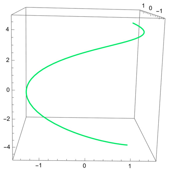
It may be observed that γ$\left(v\right)$ does not possess any singular points (Figure 3). Then, via the conditions of Equation (26), we have

$$r=1,and{\mu }_0=\frac{1}{2}ln\left|\frac{\sqrt{2}+1}{\sqrt{2}-1}\right|.$$

Figure 3. $\mathit{\gamma }\left(v\right)$ has no singular points.

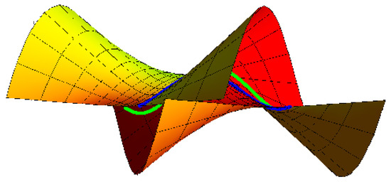
Subsequently, considering Equation (21), the striction curve is

$$\mathbf{x}\left(v\right)=\left((-1+\sqrt{2})cosv+sinv,(1-\sqrt{2})sinv+cosv,1+\sqrt{2}v\right),$$

The $\mathcal{T}like$ $\mathcal{CI}\mathit{surface}$ M with the spine curve $\mathit{\gamma }\left(u\right)$ is obtained by

$$M:\mathbf{q}(v,\mu )=((-1+cosh\mu )cosv+sinv,(1-cosh\mu )sinv+cosv,\sqrt{2}v+sinh\mu ).$$

Singularities become manifest on the striction curve (blue), where $-\pi \le v\le \pi$, and $-2.5\le \mu \le 2.5$ (Figure 4).

Figure 4. M has different singular points along the striction curve (blue).

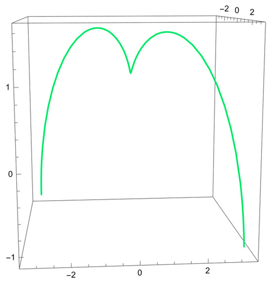
(ii) Let $\delta \left(v\right)=v$, $\eta \left(v\right)=1$, and $\sigma \left(v\right)=0$. Then ${\mathit{\gamma }}^{\prime }\left(v\right)=v$$\mathit{\chi }$${}_1\left(v\right)+$$\mathit{\chi }$${}_3\left(v\right)$. Similarly, we derive

$$\mathit{\gamma }\left(v\right)=(-vcosv+sinv,vsinv+cosv,v),$$

which has a cusp at $v=0$ (Figure 5). The striction curve is

$$\mathbf{x}\left(v\right)=\left(\right(r-v)cosv+sinv,(-r+v)sinv+cosv,v).$$

Figure 5. $\mathit{\gamma }\left(v\right)$ has a cusp at $v=0$.

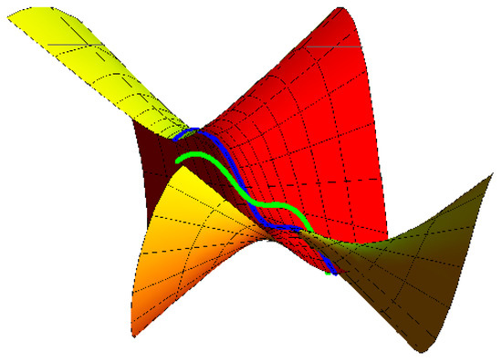
The $\mathcal{T}like$ $\mathcal{CI}surface$ with the spine curve $\mathit{\gamma }\left(v\right)$ is

$$M:\mathbf{q}(v,\mu )=\left(\right(-v+rcosh\mu )cosv+sinv,(v-rcosh\mu )sinv+cosv,v+rcosh\mu ).$$

Singularities appear on the striction curve (blue), where $r=1$, $-\pi \le v\le \pi$, and $-2.5\le \mu \le 2.5$ (Figure 6).

Figure 6. M has different singular points along the striction curve (blue).

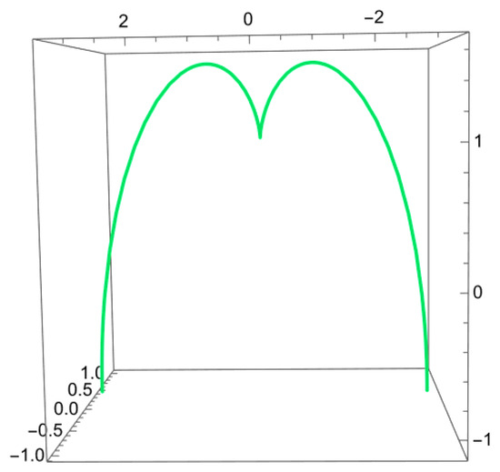
(iii) If $\delta \left(v\right)=v$ and $\sigma \left(v\right)=\eta \left(v\right)=0$, then we have ${\mathit{\gamma }}^{\prime }\left(v_0\right)=v$${\mathit{\chi }}_1\left(v\right)$, which is a $\mathcal{S}like$. By the integration, we obtain

$$\mathit{\gamma }\left(v\right)=(-vcosv+sinv,vsinv+cosv,0),$$

which contains a cusp point at $v_0=0$ (Figure 7). The $\mathcal{T}like$ canal $\mathcal{CI}\mathit{surface}$ with the spine curve$\mathit{\gamma }$$\left(v\right)$ is given by

$$M:\mathbf{q}(v,\mu )=\left(\right(-v+rcosh\mu )cosv+sinv,(v-rcosh\mu )sinv+cosv,rsinh\mu ).$$

Figure 7. $\mathit{\gamma }\left(v\right)$ has a cusp at $v=0$.

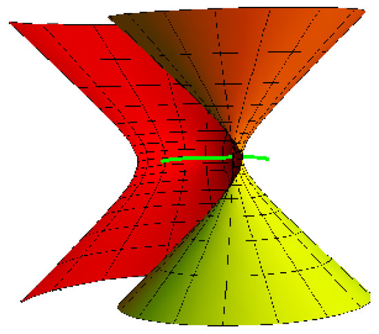
The existence of a singular point at $(v_0,{\mu }_0)=(0,0)$ on the $\mathcal{T}like$ $\mathcal{CI}\mathit{surface}$ M can be easily observed by Situation (B) of singularity. For $r=1$, $-\pi \le v\le \pi$, and $-2.5\le \mu \le 2.5$ the surface is explained in Figure 8.

Figure 8. M has a singular point at $(0,0)$.

3.3. Timelike Roller Coaster Surfaces

$\mathcal{T}like$ $\mathcal{RCO}\mathit{surfaces}$ are appointed to be those for which the tangent vector of spine curve $\mathit{\gamma }$ is lying in the Lorentzian circle plane at each point of $\mathit{\gamma }$. This signifies that $\delta \left(v\right)=\eta \left(v\right)=0$ or $\delta \left(v\right)=\sigma \left(v\right)=0$. We will take $\delta \left(v\right)=\sigma \left(v\right)=0$, and $\eta \left(v\right)\ne 0$. If so, such a surface is a $\mathcal{T}like$ $\mathcal{RCO}\mathit{surface}$ with a $\mathcal{T}like$ spine curve, that is, ${\mathit{\gamma }}^{\prime }\left(v\right)=\eta \left(v\right)$$\mathit{\chi }$${}_3\left(v\right)$. Then, the norm $∥{\mathbf{q}}_v\times {\mathbf{q}}_{\mu }∥$ can be specified by

$$∥{\mathbf{q}}_v\times {\mathbf{q}}_{\mu }∥=rsinh\mu \sqrt{{\eta }^2-r^2}.$$

(27)

From Equation (27), it follows that singularities only appear if $\mu =0$, and $\left|\eta \right|>r$. Then, from Equation (21), the striction curve is given by

$$\mathbf{x}\left(v\right)=\mathit{\gamma }\left(v\right)+r{\mathit{\chi }}_2\left(v\right).$$

(28)

Since $\delta \left(v\right)=\sigma \left(v\right)=0$, the Gaussian and mean curvatures are

$$K(v,\mu )=\frac{\left({\eta }^2-r^2\right)sinh\mu -r{\eta }^{\prime }}{{\left({\eta }^2-r^2\right)}^{2}sinh\mu },H(v,\mu )=\frac{\left({\eta }^2-r^2\right)(1+r^2)sinh\mu -r^2{\eta }^{\prime }}{2r{\left({\eta }^2-r^2\right)}^{3/2}sinh\mu }.$$

(29)

Equation (29) shows that the Gaussian and mean curvatures, whose simplifications make substantial use of the situation of a surface in the space, are not based on the geodesic curvature of the spherical indicatrix of $\mathit{\chi }\left(v\right)\in {\mathbb{S}}_1^2$, but only on $\mu$ and $\eta$. However, if a pencil of $\mathcal{T}like$ $\mathcal{RCO}\mathit{surfaces}$ has the identical value of $\eta \left(v\right)$, then the values of their Gaussian and mean curvatures are identical at the matching points, which is a geometrically significant observation. Hence, we may state the following:

Theorem 2. 

If a set of $\mathcal{T}like$ $\mathcal{RCO}\mathit{surfaces}$ possesses the same radii r, invariant $\eta \left(v\right)$, and its derivative ${\eta }^{\prime }\left(v\right)$, then the Gaussian curvature and principal lines at corresponding points are the same. Furthermore, it should be noted that these values are independent of the geodesic curvature of $\mathit{\chi }\left(v\right)\in {\mathbb{S}}_1^2$.

Since every generating Lorentzian circle is a principal line, the value of one principal curvature is

$${\mathit{\chi }}_1(v,\mu ):=∥{\mathbf{q}}_{\mu }\times {\mathbf{q}}_{\mu \mu }∥{∥{\mathbf{q}}_{\mu }∥}^{-3}=\frac{1}{r}.$$

The other principal curvature is

$${\mathit{\chi }}_2(v,\mu )=\frac{K(v,\mu )}{{\mathit{\chi }}_1}=\frac{\left({\eta }^2-r^2\right)sinh\mu -r{\eta }^{\prime }}{r{\left({\eta }^2-r^2\right)}^{2}sinh\mu }.$$

Therefore, it is possible to formulate the subsequent corollary:

Corollary 1. 

The principal line of a $\mathcal{T}like$ $\mathcal{RCO}\mathit{surface}$ is steady on each Lorentzian circle.

However, to conclude with the kinematic geometry of a $\mathcal{T}like$ $\mathcal{RCO}\mathit{surface}$, it is necessary to construct the Serret–Frenet ($\mathbf{SF}$) of the spine curve $\mathit{\gamma }$$\left(v\right)$. Then, let s be the arc length of the $\mathcal{T}like$ spine curve $\mathit{\gamma }\left(v\right)$ and $\eta \left(v\right)>0$, ∀$v\in \mathbb{R}$, where the $\mathbf{SF}$ frame of $\mathit{\gamma }$$\left(v\right)$ can be represented as

$${\mathit{\upsilon }}_1={\mathit{\gamma }}^{\prime }{∥{\mathit{\gamma }}^{\prime }∥}^{-1}={\mathit{\chi }}_3,{\mathit{\upsilon }}_2\left(s\right)=\frac{d{\mathit{\upsilon }}_1}{ds}{∥\frac{d{\mathit{\upsilon }}_1}{ds}∥}^{-1}={\mathit{\chi }}_2,{\mathit{\upsilon }}_3={\mathit{\chi }}_1,$$

where

$$\begin{array}{c}-<{\mathit{\upsilon }}_1,{\mathit{\upsilon }}_1>=<{\mathit{\upsilon }}_2,{\mathit{\upsilon }}_2>=<{\mathit{\upsilon }}_3,{\mathit{\upsilon }}_3>=1,\\ {\mathit{\upsilon }}_1\times {\mathit{\upsilon }}_{\mathbf{2}}={\mathit{\upsilon }}_3,{\mathit{\upsilon }}_1\times {\mathit{\upsilon }}_3=-{\mathit{\upsilon }}_2,{\mathit{\upsilon }}_2\times {\mathit{\upsilon }}_3={\mathit{\upsilon }}_1.\end{array}$$

Then, the $\mathbf{SF}$ equations are

$$\frac{d}{ds}\left(\begin{array}{c}{\mathit{\upsilon }}_1\hfill \\ {\mathit{\upsilon }}_2\hfill \\ {\mathit{\upsilon }}_3\hfill \end{array}\right)=\left(\begin{array}{ccc}0\hfill & \kappa \left(s\right)\hfill & 0\hfill \\ \kappa \left(s\right)\hfill & 0\hfill & \tau \left(s\right)\hfill \\ 0\hfill & -\tau \left(s\right)\hfill & 0\hfill \end{array}\right)\left(\begin{array}{c}{\mathit{\upsilon }}_1\hfill \\ {\mathit{\upsilon }}_2\hfill \\ {\mathit{\upsilon }}_3\hfill \end{array}\right),$$

(30)

where

$$\kappa \left(s\right)=\frac{\alpha }{\eta },\tau \left(s\right)=-\frac{1}{\eta },\mathrm{with}\eta \ne 0.$$

(31)

From Equation (31), it follows that if $\alpha$ is steady, the $\mathcal{T}like$ spine curve $\mathit{\gamma }$$\left(s\right)$ is a helix. From Equations (6) and (30), we have

$$M:\mathbf{q}(s,\mu )=\mathit{\gamma }\left(s\right)+r\left(cosh\mu {\mathit{\upsilon }}_1\left(s\right)+sinh\mu {\mathit{\upsilon }}_2\left(s\right)\right),s\in I,\mu \in \mathbb{R}.$$

(32)

Further, the striction curve is

$$\mathbf{x}\left(s\right)=\mathit{\gamma }\left(s\right)+r{\mathit{\upsilon }}_2\left(s\right).$$

(33)

Therefore, we not only ascertain the existence of the $\mathcal{T}like$ $\mathcal{RCO}\mathit{surface}$, but we also provide a precise characterization of the surface. This has significant importance in terms of practical applications.

• Flat and Minimal $\mathcal{T}\mathit{like}$ $\mathcal{RCO}\mathbf{Surface}$

A flat surface is one with zero Gaussian curvature. For M to be a flat surface, we have

$$K(v,\mu )=0\iff \left({\eta }^2-r^2\right)sinh\mu -r{\eta }^{\prime }=0.$$

Then, for all $\mu \in I\subseteq \mathbb{R}$, we obtain

$$\frac{{\partial }^{2}K(v,\mu )}{{\partial }^2\mu }+K(v,\mu )=0\iff {\eta }^{\prime }\left(v\right)=0.$$

(34)

From Equations (31) and (34), ${\eta }^{\prime }\left(v\right)$ via the $\mathbf{SF}$ invariant becomes

$${\eta }^{\prime }\left(v\right)=0\iff \frac{1}{\tau \left(s\right)}\frac{d\tau \left(s\right)}{ds}=0.$$

Thus, in a neighborhood of all points on M, we find that $\tau \left(s\right)$ is a non-zero constant. So, a $\mathcal{T}like$ $\mathcal{RCO}\mathit{surface}$ with $K(v,\mu )=0$ is a part of a $\mathcal{T}like$ plane. Comparably, we find that M is a minimal flat surface. Thus, we have the following corollary:

Corollary 2. 

All the flat minimal $\mathcal{T}like$ $\mathcal{RCO}\mathit{surfaces}$ are subsets of Lorentzian planes.

Example 3. 

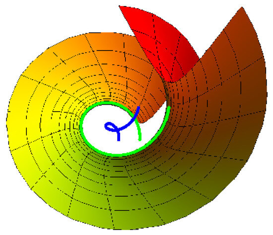
Let $\mathit{\gamma }\left(s\right)$ be a $\mathcal{T}like$ helix specified by

$$\mathit{\gamma }\left(s\right)=(acoss,asins,bs),$$

where $a>0$, $b\ne 0$, and $a^2-b^2=-1$. Then,

$$\left.\begin{array}{c}{\mathit{\upsilon }}_1\left(s\right)=(-asins,acoss,b),\\ {\mathit{\upsilon }}_2\left(s\right)=(-coss,-sins,0),\\ {\mathit{\upsilon }}_3\left(s\right)=(bsins,-bcoss,\mathit{\chi },),\\ \kappa \left(s\right)=a,\mathrm{and}\tau \left(s\right)=-b.\end{array}\right\}$$

Thus, the $\mathcal{T}like$ $\mathcal{RCO}\mathit{surface}$ pencil is

$$\mathbf{q}(s,\mu )=(acoss,asins,bs)+r(cosh\mu ,sinh\mu ,0)\times \left(\begin{array}{ccc}-asins& acoss& b\\ -coss& -sins& 0\\ bsins& -bcoss& a\end{array}\right).$$

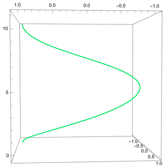
For $b=\sqrt{3}$ and $r=0.5$, $0\le s\le 2\pi$, and $-2\le \mu \le 2,$ the $\mathcal{T}like$ $\mathcal{RCO}\mathit{surface}$ with the spine curve $\mathit{\gamma }\left(s\right)$ (green) is shown in Figure 9. Singularities become evident on the striction curves (blue). It is clear that $\mathit{\gamma }\left(s\right)$ has no singular point; see Figure 10.

Figure 9. $\mathcal{T}like$ $\mathcal{RCO}\mathit{surface}$ with its spine curve (green) and striction curve (blue).

Figure 10. $\mathit{\gamma }\left(s\right)$ has no singular points.

4. Conclusions

Through the differential procedure of the mobile frame, the geometrical characteristics of the $\mathcal{T}like$ $\mathcal{CI}\mathit{surface}$ are demonstrated, and their geometrical significance is discussed. In addition, the situations for $\mathcal{T}like$ $\mathcal{RCO}\mathit{surfaces}$ to be flat or minimal surfaces are studied. Lastly, some interpretative epitomes were furnished. Additionally, interdisciplinary discussions can supply worthy unprecedented insights, but synthesizing treatises across corrections with highly assorted standards, shapes, designation, and procedures requires an appropriate approach. Recently, there has been a growth of noteworthy studies that explore various topics such as symmetry, the analysis of molecular cluster geometry, submanifold theory, singularity theory, eigenproblems, and related subjects [21,22,23,24,25,26,27,28,29]. In future works, we plan to investigate the $\mathcal{T}like$ $\mathcal{CI}\mathit{surfaces}$ and their singularities in order to enhance the results presented in this paper. We will also explore the approaches and results discussed in [26,27,28,29] to further improve our analysis.

References

- Carmo, M.P.D. Differential Geometry of Curves and Surfaces; Prentice-Hall: Englewood Cliffs, NJ, USA, 1976. [Google Scholar]
- Spivak, M.A. Comprehensive Introduction to Differential Geometry, 2nd ed.; Publish or Perish: Houston, TX, USA, 1979. [Google Scholar]
- Mc-Nertney, L.V. One-Parameter Families of Surfaces with Constant Curvature in Lorentz Three-Space. Ph.D. Thesis, Brown University, Providence, RI, USA, 1980. [Google Scholar]
- Walfare, J. Curves and Surfaces in Minkowski Space. Ph.D. Thesis, K.U. Leuven, Faculty of Science, Leuven, Belgium, 1995. [Google Scholar]
- Lopez, R. Differential Geometry of Curves and Surfaces in Lorentz-Minkowski Space. arXiv 2008, arXiv:0810.3351. [Google Scholar] [CrossRef]
- Izumiya, S.; Takeuchi, N. Singularities of ruled surfaces in R3. Math. Proc. Camb. Phil. Soc. 2001, 130, 1–11. [Google Scholar] [CrossRef]
- Izumiya, S. Special curves and ruled surfaces. Contrib. To Algebra Geom. 2003, 44, 203–212. [Google Scholar]
- Dillen, F.; Sodsiri, W. Ruled surfaces of Weingarten type in Minkowski 3-space. J. Geom. 2005, 83, 10–21. [Google Scholar] [CrossRef]
- Dillen, F.; Sodsiri, W. Ruled surfaces of Weingarten type in Minkowski 3-space, II. J. Geom. 2005, 84, 37–44. [Google Scholar] [CrossRef]
- Abdel-Baky, R.A.; Abd-Ellah, H.N. Ruled W-surfaces in Minkowski 3-space . Arch. Math. 2008, 44, 251–263. [Google Scholar]
- Zhang, X.P.; Che, W.j.; Paul, J.C. Computing lines of curvature for implicit surfaces. Comput. Aided Geom. Des. 2009, 26, 923–940. [Google Scholar] [CrossRef]
- Li, C.-Y.; Wang, R.-H.; Zhu, C.-G. Parametric representation of a surface pencil with a common line of curvature. Comput.-Aided Des. 2011, 43, 1110–1117. [Google Scholar] [CrossRef]
- Li, C.-Y.; Wang, R.-H.; Zhu, C.-G. An approach for designing a developable surface through a given line of curvature. Comput.-Aided Des. 2013, 45, 621–627. [Google Scholar] [CrossRef]
- Blum, R. Circles on Surfaces in the Euclidean 3-Space; Lecture Notes in Mathematics; Springer: Berlin/Heidelberg, Germany, 2005; Volume 792, pp. 213–221. [Google Scholar]
- Ro, J.S.; Yoon, D.W. Tubes of Weingarten types in Euclidean 3-space. J. Chungcheong Math. Soc. 2009, 22, 359–366. [Google Scholar] [CrossRef][Green Version]
- Xu, Z.; Feng, R.S. Analytic and algebraic properties of canal surfaces. J. Comput. Appl. Math. 2006, 195, 220–228. [Google Scholar] [CrossRef]
- Izumiya, S.; Saji, K.; Takeuchi, N. Circular surfaces. Adv. Geom. 2007, 7, 295–313. [Google Scholar] [CrossRef]
- Cui, L.; Wang, D.L.; Dai, J.S. Kinematic geometry of circular surfaces with a fixed radius based on Euclidean invariants. ASME J. Mech. 2009, 131, 101009. [Google Scholar] [CrossRef]
- Abdel-Baky, R.A.; Unlütürk, Y. On the curvatures of spacelike circular surface. Kuwait J. Sci. 2016, 43. [Google Scholar]
- Saad, M.K.; Ansari, A.Z.; Akram, M.; Alharbi, F. Spacelike surfaces with a common line of curvature in Lorentz-Minkowski 3-space. Wseas Trans. Math. 2021, 20, 207–217. [Google Scholar] [CrossRef]
- Sharma, J.R.; Kumar, S.; Jäntschi, L. On a class of optimal fourth order multiple root solvers without using derivatives. Symmetry 2019, 11, 1452. [Google Scholar] [CrossRef]
- Joita, D.M.; Tomescu, M.A.; Bàlint, D.; Jäntschi, L. An Application of the Eigenproblem for Biochemical Similarity. Symmetry 2021, 13, 1849. [Google Scholar] [CrossRef]
- Jäntschi, L. Introducing Structural Symmetry and Asymmetry Implications in Development of Recent Pharmacy and Medicine. Symmetry 2022, 14, 1674. [Google Scholar] [CrossRef]
- Jäntschi, L. Binomial Distributed Data Confidence Interval Calculation: Formulas, Algorithms and Examples. Symmetry 2022, 14, 1104. [Google Scholar] [CrossRef]
- Jäntschi, L. Formulas. Algorithms and Examples for Binomial Distributed Data Confidence Interval Calculation: Excess Risk, Relative Risk and Odds Ratio. Mathematics 2021, 9, 2506. [Google Scholar] [CrossRef]
- Yanlin Li, F. Mofarreh and R.A. Abdel-Baky. Timelike circular surfaces and singularities in Minkowski 3-space. Symmetry 2022, 14, 1914. [Google Scholar]
- Abdel-Baky, R.A.; Khalifa Saad, M. Singularities of non-developable ruled surface with space-like ruling. Symmetry 2022, 14, 716. [Google Scholar] [CrossRef]
- Nazra, S.; Abdel-Baky, R.A. Singularities of non-lightlike developable surfaces in Minkowski 3-space. Mediterr. J. Math. 2023, 20, 45. [Google Scholar] [CrossRef]
- Almoneef, A.A.; Abdel-Baky, R.A. Singularity properties of spacelike circular surfaces. Symmetry 2023, 15, 842. [Google Scholar] [CrossRef]
Disclaimer/Publisher’s Note: The statements, opinions and data contained in all publications are solely those of the individual author(s) and contributor(s) and not of MDPI and/or the editor(s). MDPI and/or the editor(s) disclaim responsibility for any injury to people or property resulting from any ideas, methods, instructions or products referred to in the content. |
© 2023 by the authors. Licensee MDPI, Basel, Switzerland. This article is an open access article distributed under the terms and conditions of the Creative Commons Attribution (CC BY) license (https://creativecommons.org/licenses/by/4.0/).