Abstract
Spatial capture models are broadly used for population analysis in ecological statistics. Spatial capture models for unidentified individuals rely on data augmentation to create a zero-inflated population. The unknown true population size can be considered as the number of successes of a binomial distribution with an unknown number of independent trials and an unknown probability of success. Augmented population size is a realization of the unknown number of trials and is recommended to be much larger than the unknown population size. As a result, the probability of success of binomial distribution, i.e., the unknown probability that a hypothetical individual in the augmented population belongs to the true population, can be obtained by dividing the unknown true population size by the augmented population size. This is an inverse problem as neither the true population size nor the probability of success is known, and the accuracy of their estimates strongly relies on the augmented population size. Therefore, the estimated population size in spatial capture models is very sensitive to the size of a zero-inflated population and in turn to the estimated probability of success. This is an important issue in spatial capture models as a typical count model with censored data (unidentified and/or undetected). Hence, in this research, we investigated the sensitivity and accuracy of the spatial capture model to address this problem with the objective of improving the robustness of the model. We demonstrated that the estimated population size using the proposed enhanced capture model was more accurate in comparison with the previous spatial capture model.
Keywords:
spatial Bayesian models; virtual trap; probability of success; distance sampling; count models; unidentified individuals; data augmentation; Markov chain Monte Carlo MSC:
62P10; 62C10; 62N01; 60J05; 60J22; 60K40
1. Introduction
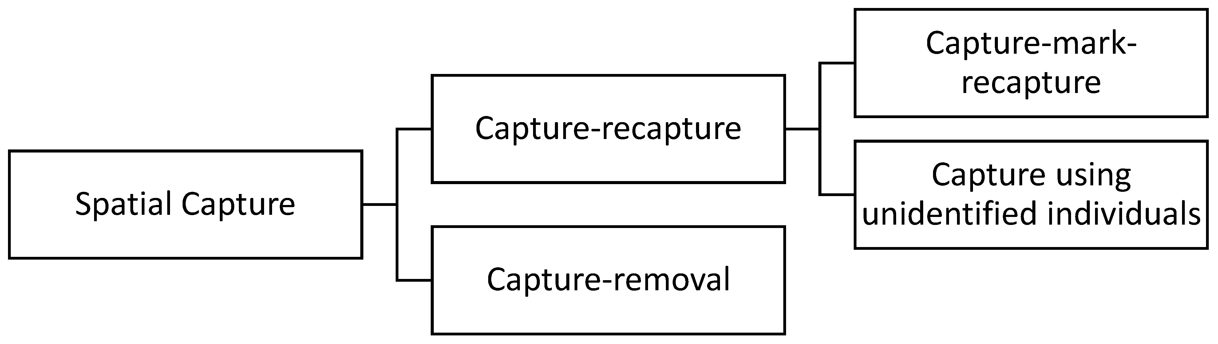
Population analysis based on spatial sampling is an emerging field of research due to its broad range of applications. Some important applications of spatial population analysis are to preserve endangered species and to control invasive species. One of the first steps required to manage a population is estimating the population size. Several methods have been developed to estimate the abundance of animals [1,2,3]. A standard approach is counting the members of the population in a random sample to estimate the population size. Population density can be then estimated by dividing the population size by the area of the animals’ habitat. The spatial capture methods can be split into two major groups, capture–removal methods and capture–recapture methods, as demonstrated in Figure 1. In capture–removal methods, the individuals that are captured will be counted, recorded, and then removed from the habitat.
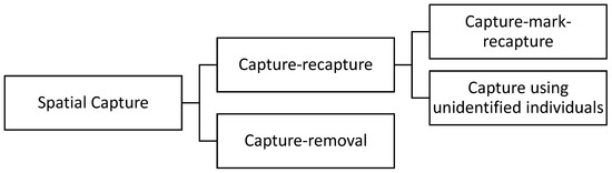
Figure 1.
Lineage of spatial capture methods.
In contrast, in capture–recapture methods, the individuals that are captured will be counted, recorded, and then released back into the habitat. Capture–recapture methods are commonly used in ecological statistics for estimating population size [1,3,4,5,6,7]. Capture–recapture methods can be split into two sub-groups, capture–mark–recapture and capture-unidentified individuals. The distinction between the two sub-groups is whether the captured individuals are marked, identified, and released, or whether individuals are virtually captured without being identified. The intuition behind the capture–mark–recapture method is that the proportion of the individuals that were captured, marked, and released in the first sample and were then recaptured in the second sample can be used to estimate the population size [1]. In the capture-unidentified-individuals method, animals are virtually captured without being identified, obtaining only the number of encountered individuals.
Capture–mark–recapture methods rely on the physical capture of individuals to collect the individual encounter history. Due to technological advances, the ability to capture individuals has been improved through more efficient methods, such as camera traps [8], acoustic recordings, and DNA samples [9,10]. Individuals can be virtually captured using their signs without being identified. Camera traps can be effectively used for the virtual capture of individuals. The inherent characteristics of sampling using camera traps include the following: (1) the same individual can be captured multiple times by the same camera, (2) the same individual can be captured by different cameras, (3) often, only a subset of individuals will be captured, and (4) captured individuals are not identified.
Conventionally, capture methods do not use spatial information about the captured individuals. Advanced spatial capture models have been implemented in the past decade [11,12,13,14,15,16]. A spatial capture model that has been broadly used was introduced by Chandler and Royle [17]. This model yields promising outcomes using unmarked or partially marked individuals to estimate the population size and density. However, due to the complexity of the spatial capture-unidentified approach, the error in the estimated population size and density could be prohibitively high. An open-ended problem is to address the shortcomings of this method and make the model robust regarding spatial sampling and spatiotemporal population analysis. The objective of this study is to improve the estimated population size by reducing the estimation error to make it robust. To this end, the proposed method performs the following tasks:
- (1)
- Employs a prior distribution for the essential parameter of the zero-inflated population;
- (2)
- Regularizes the Markov chain Monte Carlo (MCMC) by controlling the effective sample size;
- (3)
- Reduces the order of the chain by controlling the correlation of generated samples through Gibbs sampling [18,19,20].
2. Methods
The capture–recapture method is one of the most common methods to estimate the population size. The capture–recapture method has its strengths and limitations based on the species, habitat, and available resources.
2.1. Hierarchical Spatial Capture–Recapture Model
Hierarchical spatial capture–recapture (HSCR) is a statistical model widely used in wildlife ecology to estimate population size [11]. It combines information from multiple trapping sites and accounts for spatial dependences among the captured encounters to estimate the population size [21].
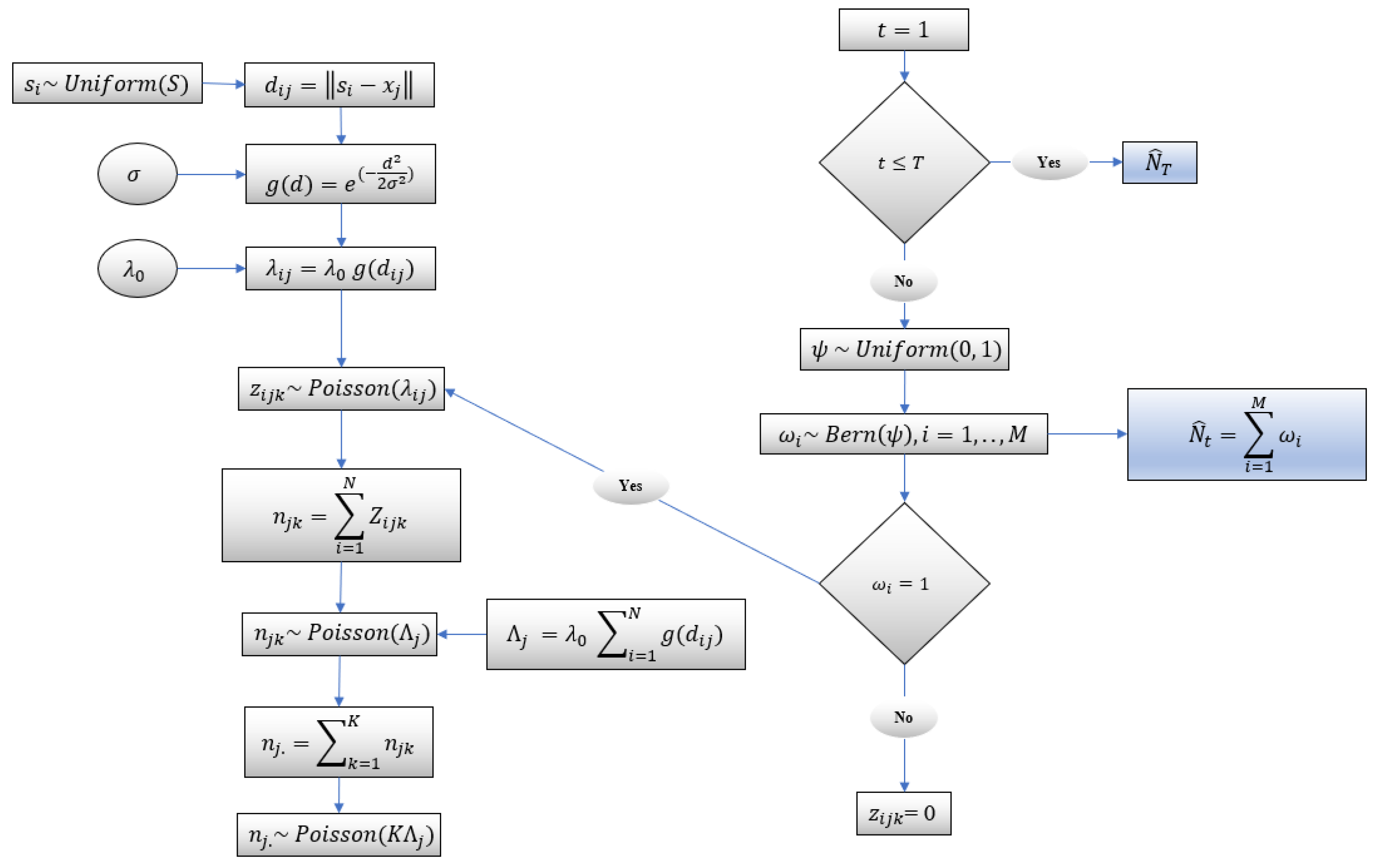
In this model, each individual is associated with an unknown spatial activity center and home range radius. Considering population size , there are unknown activity centers. It is assumed that individuals in the same habitat have the same unknown home range radius. Individual encounters in the study area are recorded using camera traps. The schematic of the capture–recapture model [22] is depicted in Figure 2 and is discussed below.
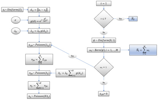
Figure 2.
Schematic of capture–recapture model.
Using distance sampling, the distance between the camera locations and the unknown center of activities is reflected in the model. It is assumed that an individual has a fixed center of activity defined with the coordinates where , and centers of activities are randomly distributed over the area of study . A bivariate uniform prior is used to model the unknown activity center :
There are camera locations; each is defined by the coordinate . Notice that an individual can be detected at multiple cameras and/or at multiple times by the same camera during a sampling occasion. A Poisson distribution is used to model a camera encounter history for individual , at camera , on occasion :
where is the encounter rate for individual at camera . The expected number of the captures or detections of an individual at camera , which is a function of the Euclidean distance between activity center and the camera location , is
where is the baseline encounter rate, and is a function of the distance which monotonically decreases and is modeled using a half Gaussian function:
where is a scale parameter and will be estimated using the collected data. If an individual can be captured once during a sampling occasion, the encounter history takes binary values; that is, takes a value of one if the individual is captured, or zero otherwise. However, an individual can be captured more than once during a sampling occasion. In this case, will be the number of times that the individual has been encountered at camera on occasion . Therefore, a encounter history matrix is considered for each individual. Obviously, the capture histories cannot be directly observed for unmarked individuals. A data augmentation method has been implemented to estimate the unknown population size. The number of camera encounters at camera on occasion is modeled by
The full conditional latent encounter data are defined by a multinomial distribution:
where . The camera encounter counts are modeled using a Poisson distribution:
where
The number of camera encounters at camera can be obtained by
Because and are independent,
In the data augmentation method used in Chandler and Royle [22], Royle et al. [17], and Royle and Dorazio [23], the camera encounter histories were augmented with a set of all-zero camera encounter histories to create a hypothetical augmented population of size in the study area. The augmented parameter is an integer and is recommended to be much greater than unknown , i.e., to avoid the truncation of the posterior distribution of . Notice that, a very large value of will increase the computational time. Uninformative prior distributions are assumed for the unknown parameters. Prior distributions of and are considered , where , probability of success, is the probability that an individual in the occupancy model of size is a member of the true population of size . A binomial prior distribution, , is assumed for where . Assuming a discrete uniform distribution for the detection of individuals in the hypothetical population of size , individuals are associated with all-zero encounter histories. In turn, indicator variables are introduced such that
where , with expected value and variance . Hence, the encounter data for each individual in the augmented population can be modeled by
and in turn, the population size can be obtained by
Assuming mutual independence of the prior distributions, the joint prior distribution is
and in turn, the joint posterior distribution of the parameters is
where is a coordinate matrix of camera locations. Notice that in the original model, the assumed prior distributions for and are uninformative. A spatial Metropolis–Gibbs Markov chain Monte Carlo (MCMC) algorithm for estimating the model parameters is used in Chandler and Royle [22].
2.2. Proposed Method
For a random sample from a given population with unknown probability distribution , the unknown parameter can be estimated using a point estimator to construct a confidence interval for the unknown parameter. In Bayesian statistics, the samples are often generated from an uninformative prior. However, an informative prior to sample parameter can be inferred empirically or could be available from previous studies [21,22,23]. In the next section, an informative prior to sample is introduced.
2.3. Sensitivity of the Model to
The probability of success that an individual is a member of the population is
where is the unknown true population size, and is the size of the zero-inflated population. In the data augmentation model, an arbitrary large zero-inflated population is generated. As a result, the upper bound of augmented population size can increase indefinitely. It has been demonstrated using simulations that by increasing the zero-inflated populationsize, the true estimation error will be increased. In turn, the spatial models can substantially overestimate the unknown population size. To address the inflated estimation error due to the inflated size of the population, we suggest bounding the size of the augmented data. A practical lower bound of the augmented data is twice as high as the unknown population size. By increasing the size of the inflated population above twice the true population size, the error of the estimated population size will increase, and in turn, the width of the credible interval will be increased.
To investigate the sensitivity of the model to , simulations were designed, and the impact of on the estimated population size was studied. In the first set of simulations, an uninformative prior with no constraints was considered to sample the probability of success . It means all values in the range of [0, 1] will be accepted for by the Gibbs sampling. In the next set of simulations, different constraints for sampling were enforced. An estimate of can be obtained by , where is sampled from a Beta distribution with parameters:
and
The estimated number of individuals, in Equation (13), is given by The expected population size at camera is given by
where is the indicator function for individual , and is the estimated probability of success, that is, the probability that an individual belongs to the true population. The variance of the estimated can be derived from
and the standard deviation of the estimated is
2.4. Autocorrelation Plot
The autocorrelation plot is an effective tool to assess the correlation of the samples produced by a Markov chain and inspect whether the samples are well mixed [24]. The correlation coefficient range is [−1, 1], with −1 indicating perfect negative correlation, zero representing no correlation, and one indicating perfect positive correlation. It will also quantify the correlation between the current value of the chain and its past values (lags). Generated samples by MCMC from one iteration to the next will be somewhat correlated. In a well-mixed chain, the correlation is small, and the autocorrelation drops relatively quickly. However, if the chain does not mix well, samples will be highly correlated, and the correlation will decay slowly. In turn, a large number of iterations is required to reach the stationary distribution of the Markov chain [25,26]. Lag autocorrelation represents the autocorrelation between the current sample and kth preceding sample [19].
2.5. Effective Sample Size
Effective sample size (ESS) is another way to study the convergence of the chain. ESS provides an estimated number of independent observations equivalent to the samples generated by a Markov chain [27] that iterates times (Figure 2). In other words, it represents the number of independent samples in the simulation and gives an estimate of how well the simulation represents the target distribution. As we have mentioned, the samples generated by MCMC are somewhat correlated. It means, less information is provided by highly correlated or poor mixing chains. A high ESS indicates a well-mixed chain, while a low ESS indicates poor convergence. A chain with a low ESS must run for a larger number of iterations to improve the convergence of the chain toward its stationary distribution [26].
3. Results
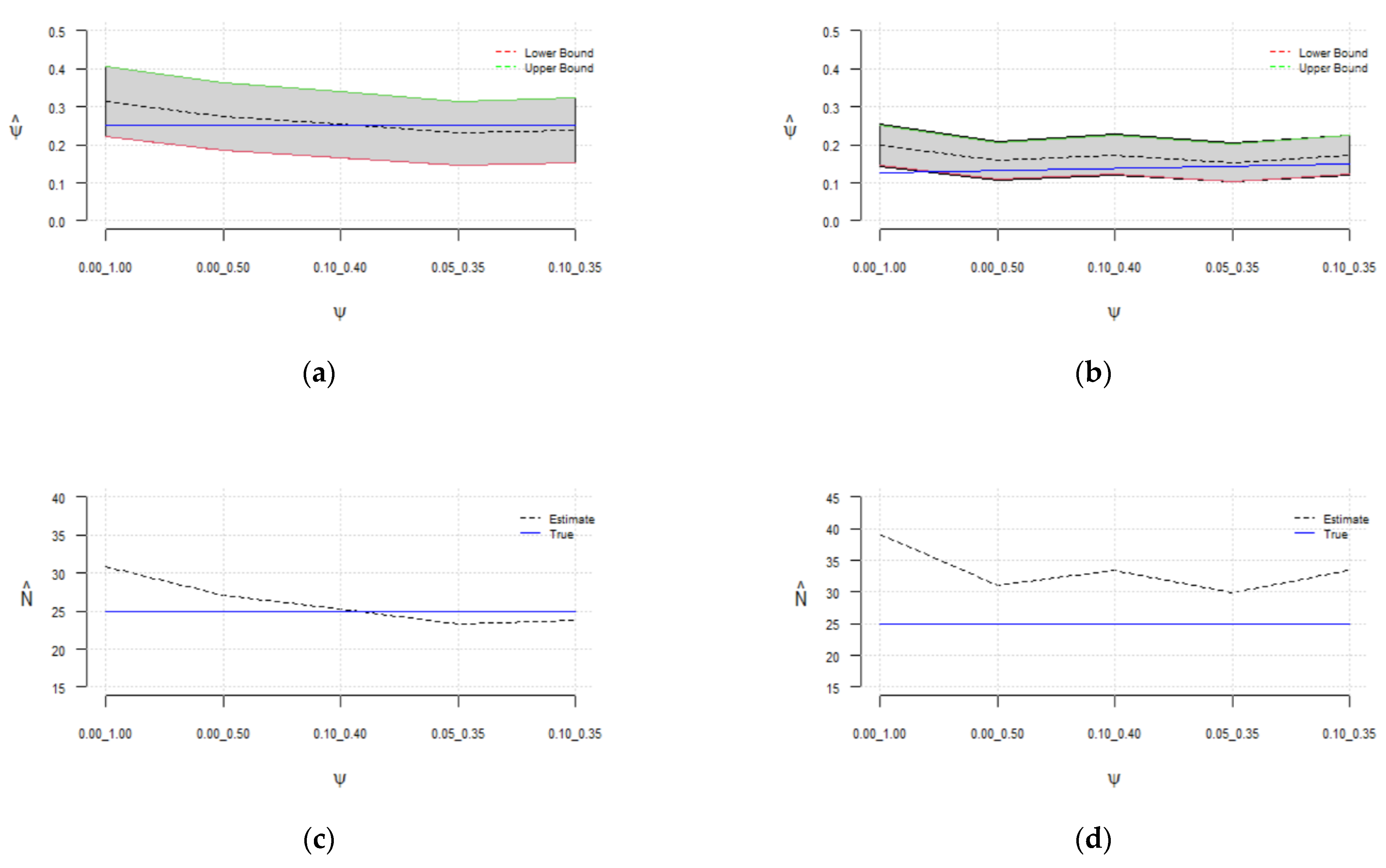
The simulations were implemented using R v4.2.2 (a statistical analysis programming language) within the RStudio and a range of specialized packages for Markov chain Monte Carlo (MCMC), the Metropolis–Hasting algorithm, and the Gibbs sampler (see [19,28,29,30,31]). Statistical simulations were implemented to study the sensitivity of the spatial capture model to the data augmentation parameter (added number of zeros) by estimating unknown population size , home range , and . In this model, a hypothetical population size () for the upper bound of the true population size () is selected such that . In turn, the estimated can assume values between zero and . Several simulations were performed to test the sensitivity of the model to the selected value of for the true value of , and the results are shown in Table 1 and Figure 3. The estimated values of , and were calculated along with the ESS and autocorrelation. The estimated population size is obtained by running simulations with and without constraint on the sampling range of (Table 1). For the true probability of success () is , and it is for .

Table 1.
Summary of the estimated mean of , and population size for different ranges of and .
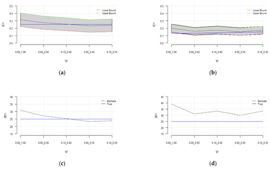
Figure 3.
Sensitivity of the estimated probability of success () to the selected range of for (a) and (b); sensitivity of the estimated population size () to the selected range of for (c) and (d).
It can be observed (in Table 1 and Figure 3) that the estimated has assumed a broad range of values. The sensitivity of the model to the added number of zeros is more noticeable when sampling the probability of success from [0, 1], i.e., without constraint. In all cases, the estimated values of are more accurate with the constraints on . It was observed that by decreasing the sampling range of the , the effective sample size will increase, while the rejection rate and in turn computational cost increase.
It is recommended to choose large values for the data augmentation parameter . However, it must be pointed out that may not be increased indefinitely, as it may produce very small close to zero and in turn significant overestimation of . Hence, two different constraints, [0.0, 0.5] and [0.1, 0.4], were set for the range of parameter , and the simulation results were compared with the uninformed prior of and sampling it from [0, 1]. We ran 50 simulations for each scenario and computed the average to be able to generalize the results.
As depicted in Figure 3, regardless of the number of added zeros , the sensitivity decreases by constraining the probability of success, and true is contained in the estimated confidence interval highlighted in gray. Furthermore, the estimated is consistent for , as depicted in Figure 2. A fair estimate of is obtained when sampling from [0.0, 0.5] regardless of . The results show that a reasonable estimate of between 23 and 33 can be obtained by constraining , and with a higher probability of success of 0.25, the estimated is more accurate (between 23 and 27).
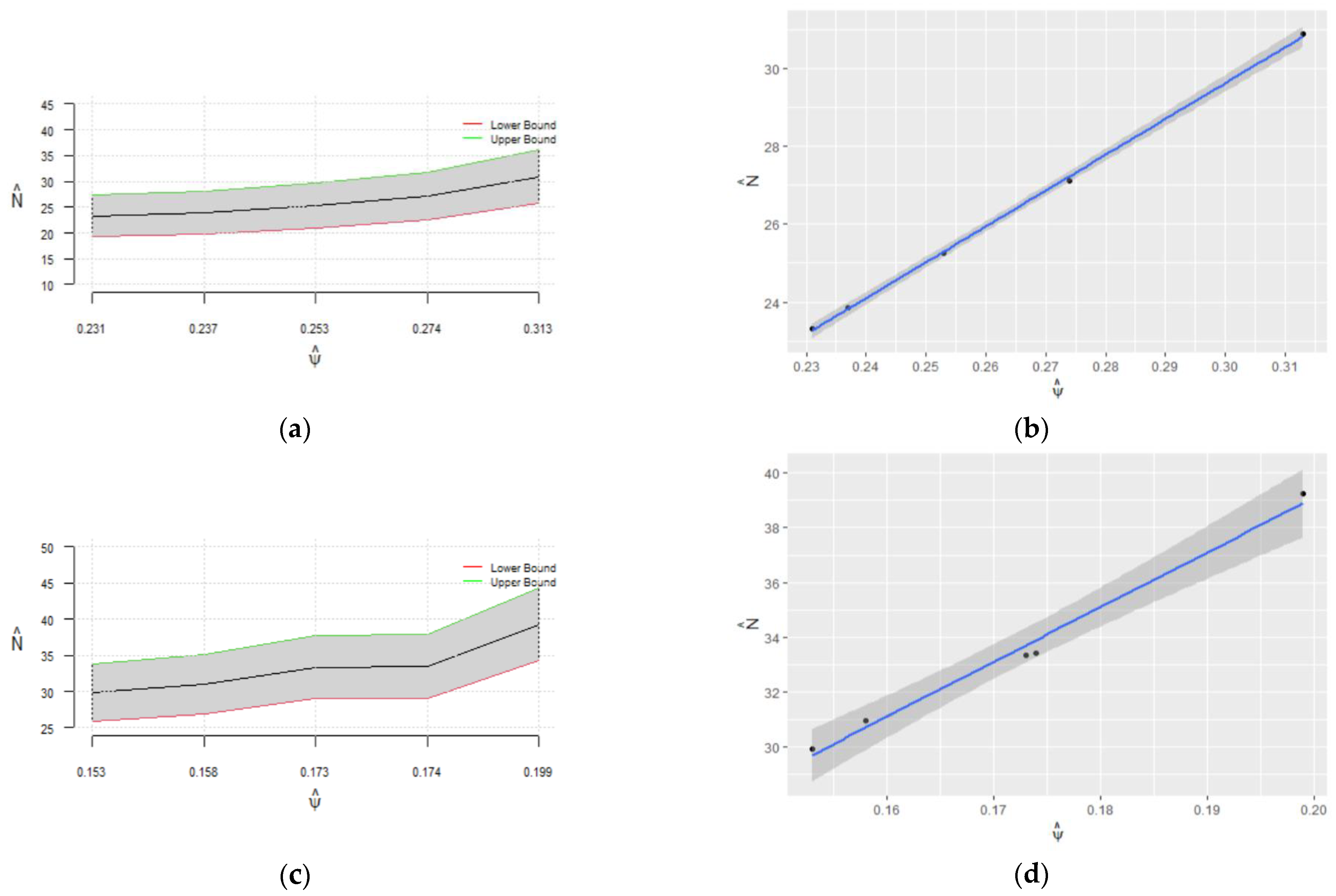
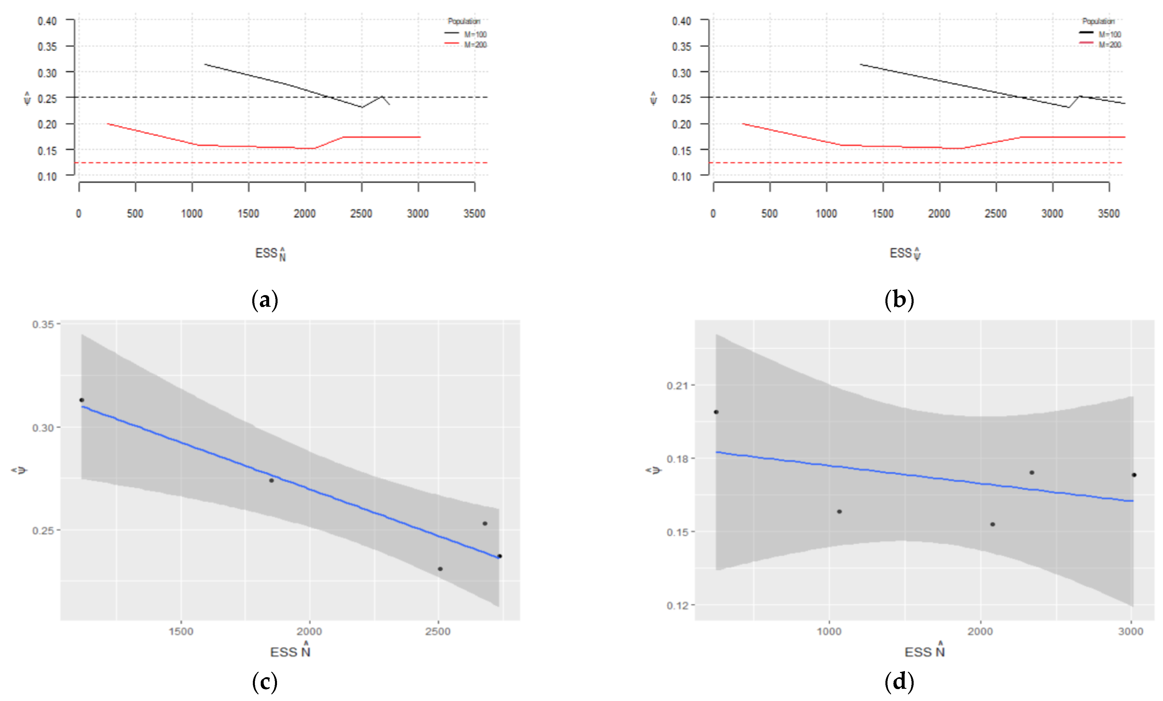
Table 2 shows the estimated values of , and , along with ESS and autocorrelation for and . For , the estimated value of the population size in the case of no constraint on the parameter is about 32, with an ESS equal to 1862. After enforcing the constraint [0, 0.5] on the range of to reject all samples with , the estimated value of is about 27 with an ESS of 4368. Moreover, by limiting the range of to [0.10, 0.40], the estimated population size is 26 with the ESS of 7678. Pointwise nonparametric confidence intervals for population size given the range of are compared for different values of (Figure 4). As we can see in this figure, more robust estimates of the population size and are obtained for , while the estimation error and bias are increased for . Figure 5 shows the estimated and its confidence interval regarding the ESS of and ESS of for different values of It is clear that the estimated is more robust and converges to its true value within an ESS of 3000 for , while it is overestimated and does not converge to the true value of for
Table 2.
Summary of 50 runs of the estimated mean of , and population size for different ranges of and .
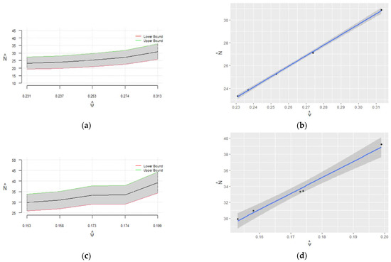
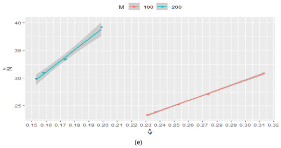
Figure 4.
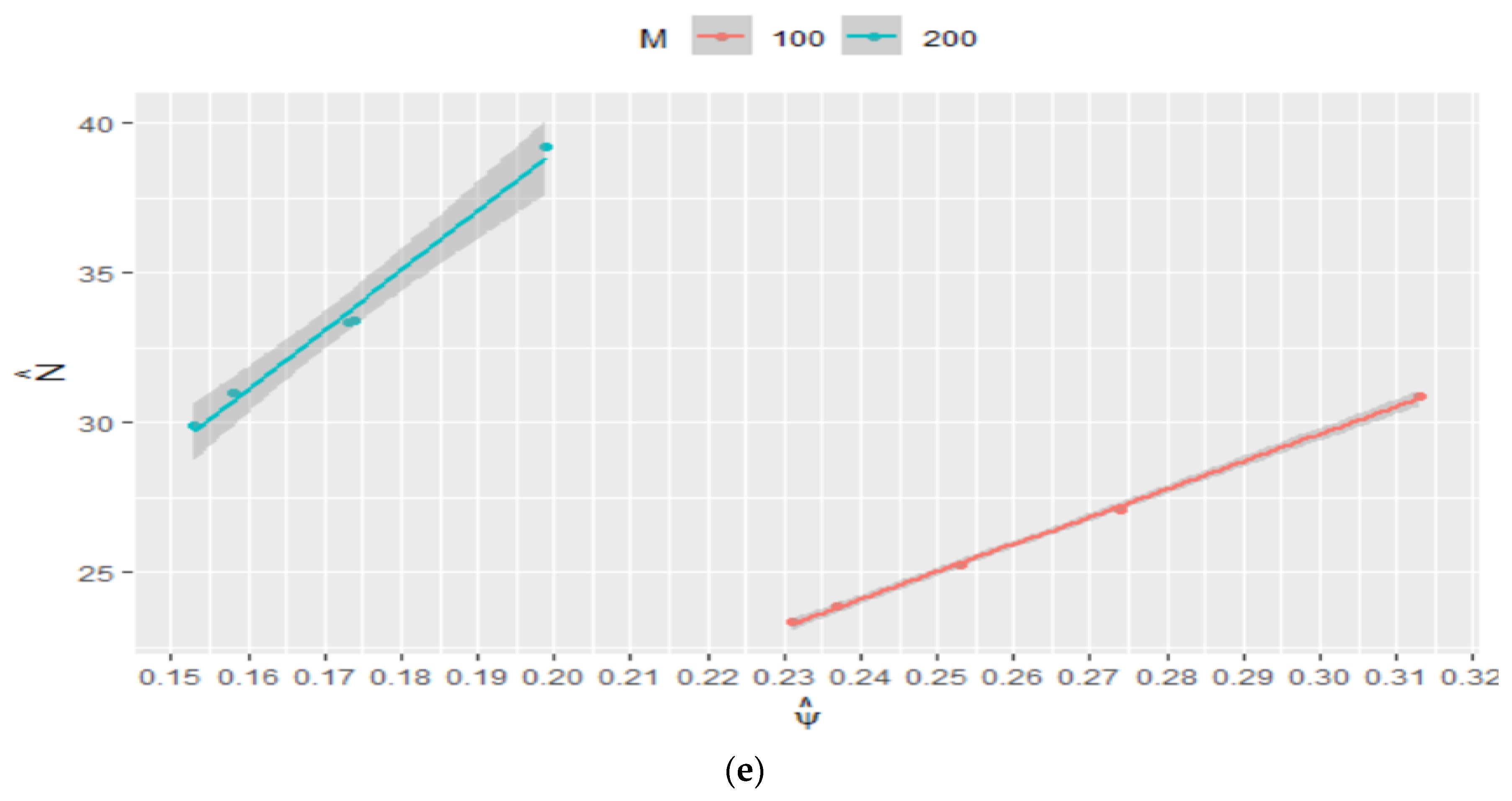
Pointwise 95% confidence intervals for regarding for (a) and (c); nonparametric 95% confidence intervals for regarding for (b) and (d); (e) combined plot of the confidence intervals in panels (b,d) for comparison.

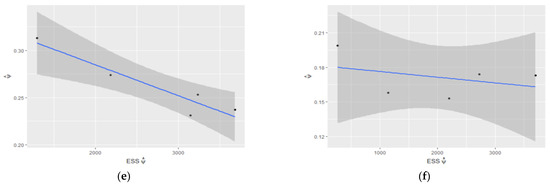
Figure 5.
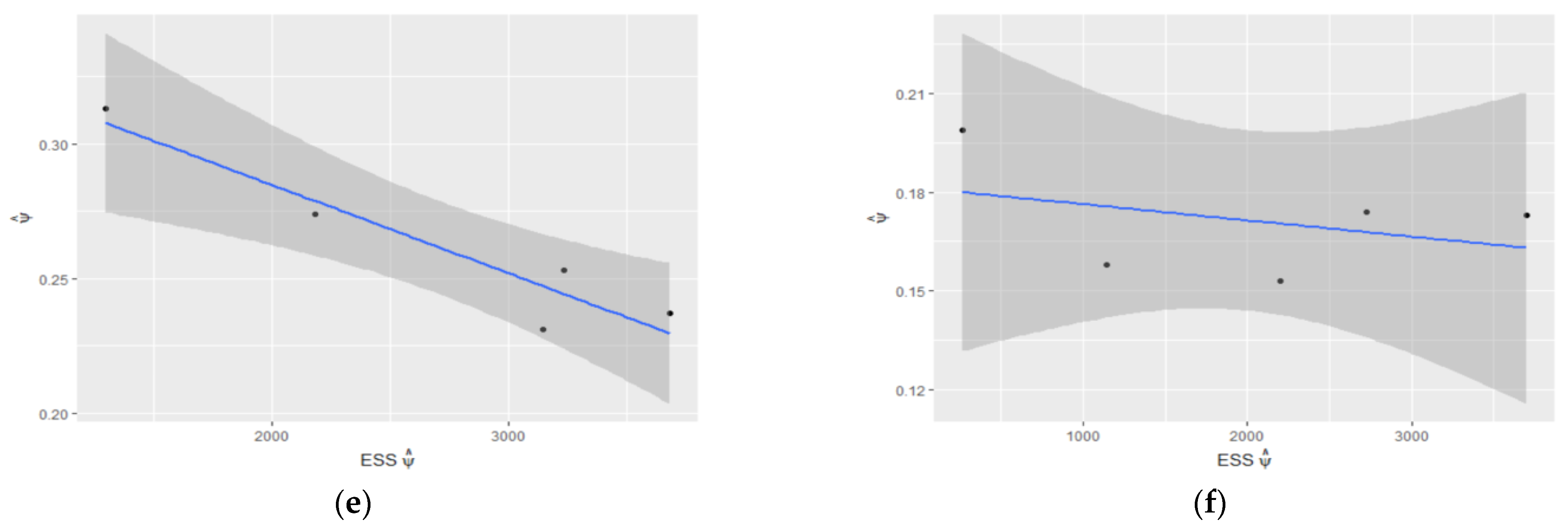
Estimated : (a) vs. ESS of and (b) vs. ESS of ; estimated 95% confidence interval for regarding ESS of for (c) and (d); estimated 95% confidence interval for regarding ESS of for (e) and for (f).
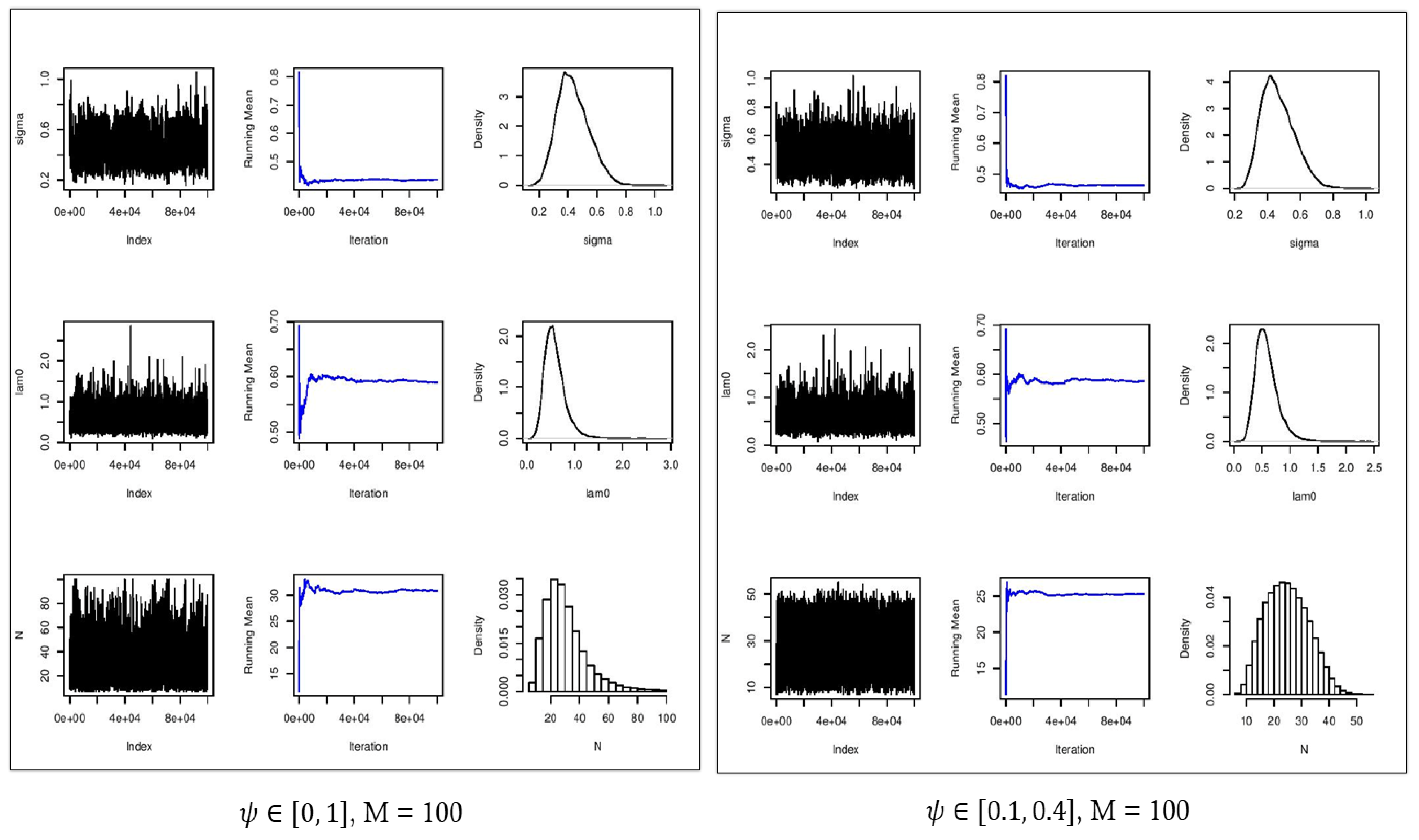
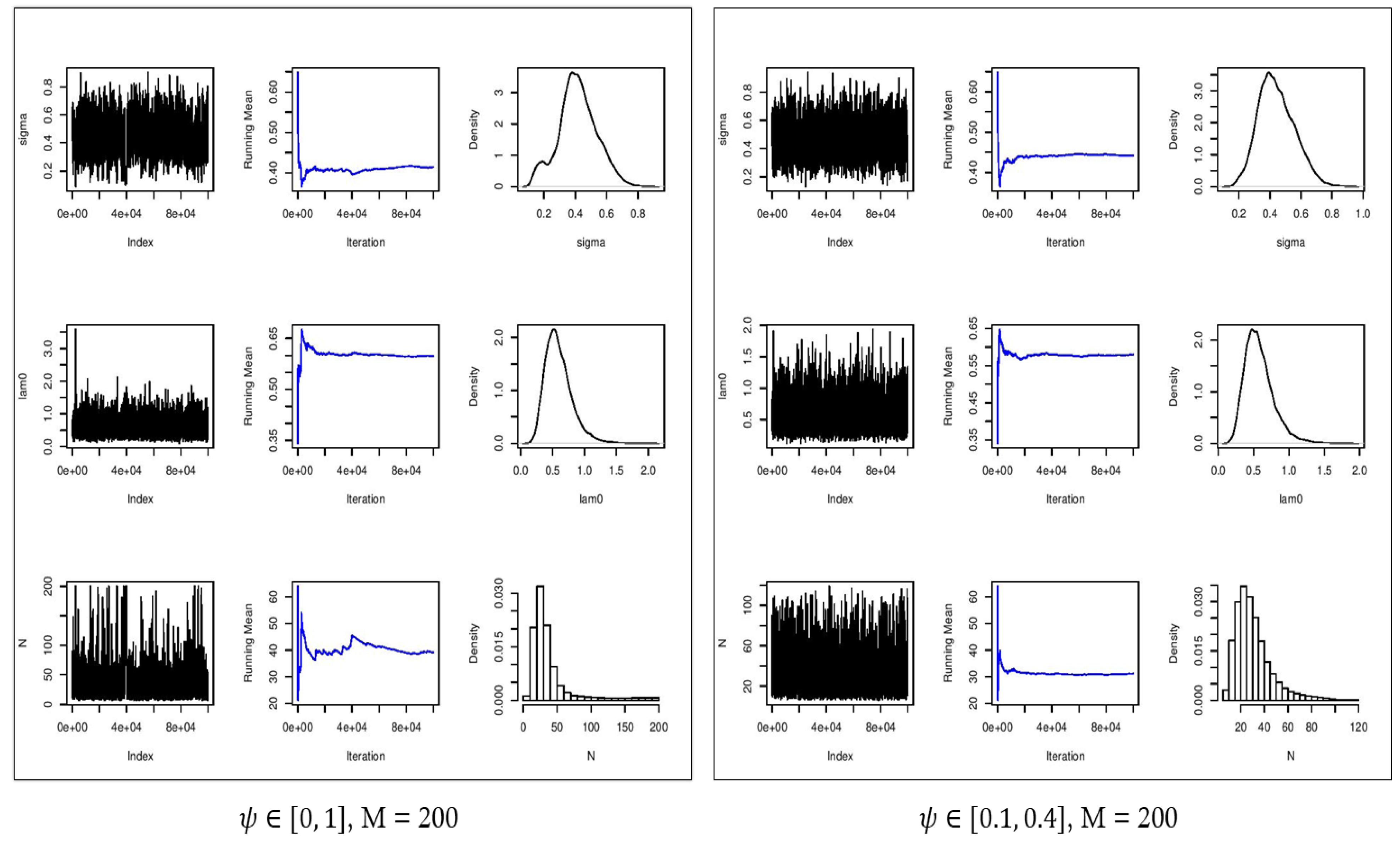
Figure 6 and Figure 7 show the estimated parameters and in comparison with their true values. In all cases, the densities of the estimated parameters converged to the stationary distribution. With the constraint on parameter , the mixing of samples in the chains were improved, providing more accurate estimates of . With no constraint on the parameter and , the Monte Carlo average of the estimated population size was about 33 with an ESS of 1779. By enforcing the constraints on the parameter , the estimated population size was 31 which demonstrated a smaller absolute error as well as improved accuracy with a narrower confidence interval in comparison with the scenario with an uninformative prior distribution (Table 2). We should point out that with , the augmented population size is eight times larger than the true population size of , as a result of which, is substantially overestimated, and is well outside of the confidence interval of [LB = 34.0,UB = 44.0] (Table 3).
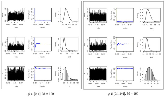
Figure 6.
Convergence plots (first column), running mean (second column), and estimated posterior densities (third column) for (first row), (second row), and (third row) for . Left: no constraint on . Right: constrained on [0.1, 0.4].
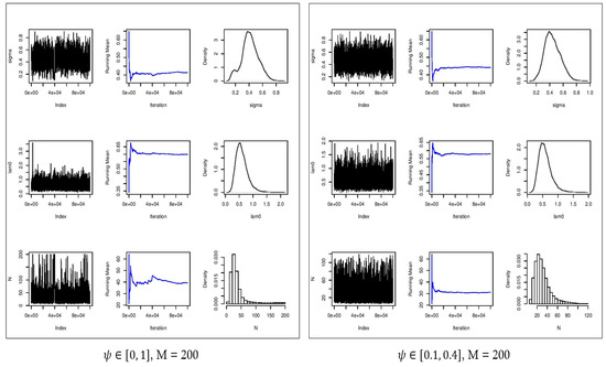
Figure 7.
Convergence plots (first column), running mean (second column), and estimated posterior densities (third column) for (first row), (second row), and (third row) for . Left: no constraint on . Right: constrained on [0.1, 0.4].
Table 3.
Estimated 95% confidence interval for population size and probability of success .
The estimated for the constrained in [0.10, 0.40] and has the minimum absolute error and provides the highest number of independent samples with generated through 90,000 MCMC iterations. With an uninformative prior for , the range of estimated is [0.30, 2.03] with an average of 0.56. By regularizing and constraining its range to [0, 0.50], the range of the estimated is [0.40, 1.70]. Moreover, by constraining to [0.10, 0.40], the range of the estimated is [0.39, 0.8] with an average of 0.52 and the narrowest range for the estimated containing true and with the lowest absolute error of the estimate. The estimated for the aforementioned ranges of is 0.497, 0.546, and 0.557, respectively. The estimated population size ranges from 8 to 61 with an average of 32 for no restriction on , from 6 to 37 with an average of 27 for belongs to [0, 0.50], and from 16 to 37 with an average of 26 for belongs to [0.1, 0.40]. The estimated value of the population size is more accurate, and the range of the estimated value is narrower after regularizing (Table 1, Table 2 and Table 3). Moreover, the standard error for the estimated population size ranges from 5.8 to 24.7, with an average of 14.37 with no restriction on . The standard error is between 5.8 and 13 with an average of 8.56 for . With constrained between 0.10 and 0.40, the standard error ranges from 5 to 9 with an average of 6.8.
The estimated values for with = 200 are 0.546, 0.527, and 0.496 (Table 2) for all three scenarios regarding , i.e., no constraint, [0, 0.5], and [0.1, 0.4]. Also, the estimated values of are 0.527, 0.564, and 0.545 (Table 2) for the aforementioned constraints on . As it can be observed, the range of the estimated parameter is smaller with a constraint on (Table 1 and Table 2). The estimated population size ranges from 6 to 107 with an average of 33 with no constraint on , from 11 to 61 with an average of 31 by constraining to [0, 0.5], and from 19 to 47 with an average of 31 by constraining to [0.10, 0.40]. As depicted in Figure 7, we can see that by constraining to [0.10, 0.40], the distribution of has a shorter tail and converges to the stationary posterior distribution. Moreover, there is better mixing of the chains providing more accurate estimates of the parameters.
4. Discussion
By constraining the parameter to the range [0, 0.50], can assume any value greater than (). In contrast, by restricting to the range [0.10, 0.40], is double-bounded within . Enforcing an upper bound of is a sufficient assumption that satisfies recommended for spatial capture models, while we prevent indefinitely large that can result in prohibitively small estimates of (close to zero) with a highly skewed distribution. In practical applications, determining an accurate prediction for the value of can be challenging. In cases where no prior information about is known, the range [0, 0.5] can be considered for . However, if prior information about the population size is known, and the camera grid provides adequate coverage of the habitat of interest, the range [0.1, 0.4] for is preferred to avoid underestimation of toward zero.
It was observed that the estimated population size using the spatial capture models with camera encounters is subject to overestimation and bias. The estimation bias tends to increase by increasing . ESS and lag 10 can be used to control the convergence of MCMC and in turn controling the estimation bias. Specifically, lower ESS values are associated with higher bias, whereas higher ESS values are associated with lower bias. Additionally, larger values of lag 10 tend to correspond to higher levels of bias, and vice versa.
In terms of , by setting it within five times of the estimated is relatively accurate with low bias, while by increasing toward 10 times of the estimated converges to higher values (overestimates) with increased bias. It should be noticed that the values of and depend on each other, and in turn, their estimated values are not mutually exclusive. Specifically, there is a trade-off between the two estimated parameters. If the estimate of increases, the estimates of will decrease, and vice versa. Potentially, the estimated population size could be further improved by considering a prior distribution for , which is the subject of our future work. Nonetheless, regularizing the value of by a prior distribution in conjunction with controlling the ESS and log 10 improved the accuracy of the estimated population size.
5. Conclusions
Population management is important to preserve the populations of endangered species and to control the populations of invasive species. Estimating the population size is an essential task in managing the population. Collecting a random sample of individuals from the population is a feasible practice to study the population when it is not possible to count every individual. Capture–recapture methods based on spatial sampling and count models have become the standard methods in the analytical framework for ecological statistics and are widely used for population analysis to estimate population size and density.
The unknown size of a population is considered as the number of successes in a binomial distribution. The parameters of this binomial distribution are an unknown number of independent trials and an unknown probability of success. This is an inverse problem as none of the parameters including the population size, the probability of success, and the number of independent trials is known. An initial realization of the unknown number of trials is required to approach a solution while the accuracy of the estimated parameters strongly relies on the initial value for the zero-inflated population size. Hence, the estimated population size in spatial capture models is quite sensitive to the size of a zero-inflated population and in turn to the estimated probability of success. This is a typical count model with censored data as captured individuals are not identified, and some individuals are not detected. To address this problem and improve the estimation accuracy, in this research, we investigated the sensitivity and accuracy of the spatial capture-unidentified models (using virtual encounters) with the objective of improving their robustness. Statistical simulations were implemented to study the sensitivity of the spatial capture models to the zero-inflated population parameter .
In capture-unidentified models, augmented population size () is allowed to be increased indefinitely, and so will be allowed to belong to [0, 1]. As a result, the population size will be highly overestimated, and the accuracy of the estimate declines for large values of while the estimated moves toward zero. Consequently, the credible interval becomes wider, and the distribution of displays a heavy and long right tail. Moreover, the true estimation error and estimation bias increase, while ESS tends to remain low. To address the aforementioned issues, a lower and an upper bound for were recommended to prevent overestimation of population size that is caused by excessive underestimation of when it is not regularized. In this way, the accuracy and bias were retained providing fairly narrow credible intervals, while ESS was improved.
Author Contributions
Conceptualization, M.J., F.H., R.D.B. and N.N.K.; methodology, M.J., F.H., R.D.B. and N.N.K.; software, M.J., F.H., R.D.B. and N.N.K.; validation, M.J., F.H., R.D.B. and N.N.K.; formal analysis, M.J. and F.H.; investigation, M.J., F.H., R.D.B. and N.N.K.; resources, N.N.K.; data curation, M.J., F.H. and R.D.B.; writing—original draft preparation, M.J., F.H., R.D.B. and N.N.K.; writing—review and editing, M.J., F.H., R.D.B. and N.N.K.; visualization, M.J., F.H., R.D.B. and N.N.K.; supervision, N.N.K.; project administration, N.N.K. All authors have read and agreed to the published version of the manuscript.
Funding
This research received no external funding.
Data Availability Statement
No data was collected. Rather, data was randomly sampled in the simulation study.
Conflicts of Interest
The authors declare no conflict of interest.
Abbreviations
| MCMC | Markov chain Monte Carlo |
| HSCR | Hierarchical spatial capture–recapture |
| Population size | |
| Estimated population size | |
| Sampling occasion | |
| Camera encounter history for individual , at camera , on occasion | |
| The encounter rate for individual at camera | |
| The baseline encounter rate | |
| Home range radius. | |
| The Euclidean distance between activity center and the camera location | |
| The number of camera encounters at camera on occasion | |
| The augmented parameter (the total number of hypothetical individuals) | |
| Probability of success, i.e., the probability that an individual in the occupancy model of size is a member of the original model of size | |
| and | Parameters of Beta probability distribution |
| ESS | The effective sample size |
| The number of zeros added to the model (data augmentation size) | |
| The autocorrelation between the current sample and kth preceding sample |
References
- Pollock, K.H. Capture-Recapture Models: A Review of Current Methods, Assumptions and Experimental Design. Stud. Avian Biol. 1981, 6, 426–435. [Google Scholar]
- Schwarz, C.J.; Seber, G.A. Estimating Animal Abundance: Review III. Stat. Sci. 1999, 14, 427–456. [Google Scholar] [CrossRef]
- Nichols, J.D. Capture-Recapture Models. BioScience 1992, 42, 94–102. [Google Scholar] [CrossRef]
- Pollock, K.H. A Capture-Recapture Design Robust to Unequal Probability of Capture. J. Wildl. Manag. 1982, 46, 752–757. [Google Scholar] [CrossRef]
- Pollock, K.H.; Nichols, J.D.; Brownie, C.; Hines, J.E. Statistical Inference for Capture-Recapture Experiments. Wildl. Monogr. 1990, 48, 3–97. [Google Scholar]
- Karanth, K.U. Estimating Tiger Panthera Tigris Populations from Camera-Trap Data Using Capture—Recapture Models. Biol. Conserv. 1995, 71, 333–338. [Google Scholar] [CrossRef]
- O’Connell, A.F.; Nichols, J.D.; Karanth, K.U. Camera Traps in Animal Ecology: Methods and Analyses; Springer: Berlin/Heidelberg, Germany, 2011; Volume 271. [Google Scholar]
- Jaber, M.; Woesik, R.V.; Kachouie, N.N. Probabilistic Detection Model for Population Estimation; Old Dominion University: Norfolk, VA, USA, 2018; p. 43. [Google Scholar]
- Distiller, G.; Borchers, D.L. A spatially explicit capture–recapture estimator for single-catch traps. Ecol. Evol. 2015, 5, 5075–5087. [Google Scholar] [CrossRef]
- Engeman, R.; Massei, G.; Sage, M.; Gentle, M.N. Monitoring Wild Pig Populations: A Review of Methods. Environ. Sci. Pollut. Res. 2013, 20, 8077–8091. [Google Scholar] [CrossRef]
- Royle, J.A.; Young, K.V. A Hierarchical Model for Spatial Capture–Recapture Data. Ecology 2008, 89, 2281–2289. [Google Scholar] [CrossRef]
- Royle, J.A.; Karanth, K.U.; Gopalaswamy, A.M.; Kumar, N.S. Bayesian Inference in Camera Trapping Studies for a Class of Spatial Capture–Recapture Models. Ecology 2009, 90, 3233–3244. [Google Scholar] [CrossRef]
- Kery, M.; Gardner, B.; Stoeckle, T.; Weber, D.; Royle, J.A. Use of Spatial Capture-recapture Modeling and DNA Data to Estimate Densities of Elusive Animals. Conserv. Biol. 2011, 25, 356–364. [Google Scholar] [CrossRef] [PubMed]
- Borchers, D. A Non-Technical Overview of Spatially Explicit Capture–Recapture Models. J. Ornithol. 2012, 152, 435–444. [Google Scholar] [CrossRef]
- Royle, J.A.; Chandler, R.B.; Sollmann, R.; Gardner, B. Spatial Capture-Recapture; Academic Press: Cambridge, MA, USA, 2013; ISBN 0-12-407152-X. [Google Scholar]
- Gardner, B.; Reppucci, J.; Lucherini, M.; Royle, J.A. Spatially Explicit Inference for Open Populations: Estimating Demographic Parameters from Camera-trap Studies. Ecology 2010, 91, 3376–3383. [Google Scholar] [CrossRef] [PubMed]
- Royle, J.A.; Dorazio, R.M.; Link, W.A. Analysis of Multinomial Models with Unknown Index Using Data Augmentation. J. Comput. Graph. Stat. 2007, 16, 67–85. [Google Scholar] [CrossRef]
- Jiao, G.; Liang, J.; Wang, F.; Chen, X.; Chen, S.; Li, H.; Jin, J.; Cai, J.; Zhang, F. Longitudinal Data Analysis Based on Bayesian Semiparametric Method. Axioms 2023, 12, 431. [Google Scholar] [CrossRef]
- Carlo, C.M. Markov Chain Monte Carlo and Gibbs Sampling. Lect. Notes EEB 2004, 581, 3. [Google Scholar]
- Alotaibi, R.; Nassar, M.; Elshahhat, A. Statistical Analysis of Inverse Lindley Data Using Adaptive Type-II Progressively Hybrid Censoring with Applications. Axioms 2023, 12, 427. [Google Scholar] [CrossRef]
- Sollmann, R.; Tôrres, N.M.; Furtado, M.M.; de Almeida Jácomo, A.T.; Palomares, F.; Roques, S.; Silveira, L. Combining Camera-Trapping and Noninvasive Genetic Data in a Spatial Capture–Recapture Framework Improves Density Estimates for the Jaguar. Biol. Conserv. 2013, 167, 242–247. [Google Scholar] [CrossRef]
- Chandler, R.B.; Royle, J.A. Spatially explicit models for inference about density in unmarked or partially marked populatioins. Ann. Appl. Stat. 2013, 7, 936–954. [Google Scholar] [CrossRef]
- Royle, J.A.; Dorazio, R.M. Parameter-Expanded Data Augmentation for Bayesian Analysis of Capture–Recapture Models. J. Ornithol. 2012, 152, 521–537. [Google Scholar] [CrossRef]
- Christensen, O.F.; Roberts, G.O.; Sköld, M. Robust Markov Chain Monte Carlo Methods for Spatial Generalized Linear Mixed Models. J. Comput. Graph. Stat. 2006, 15, 1–17. [Google Scholar] [CrossRef]
- Kuzmanovska, I. Markov Chain Monte Carlo Methods in Biological Mechanistic Models. 2012. Available online: https://www.research-collection.ethz.ch/handle/20.500.11850/153590 (accessed on 8 August 2023).
- Lewis, A. Efficient Sampling of Fast and Slow Cosmological Parameters. Phys. Rev. D 2013, 87, 103529. [Google Scholar] [CrossRef]
- Martino, L.; Elvira, V.; Louzada, F. Effective Sample Size for Importance Sampling Based on Discrepancy Measures. Signal Process. 2017, 131, 386–401. [Google Scholar] [CrossRef]
- Fabreti, L.G.; Höhna, S. Convergence Assessment for Bayesian Phylogenetic Analysis Using MCMC Simulation. Methods Ecol. Evol. 2022, 13, 77–90. [Google Scholar] [CrossRef]
- Zhang, J.; Cui, S. Investigating the Number of Monte Carlo Simulations for Statistically Stationary Model Outputs. Axioms 2023, 12, 481. [Google Scholar] [CrossRef]
- Jaber, M. A Spatiotemporal Bayesian Model for Population Analysis. 2022. Available online: https://repository.fit.edu/etd/880/ (accessed on 8 August 2023).
- Martin, A.D.; Quinn, K.M.; Park, J.H. MCMCpack: Markov Chain Monte Carlo in R. J. Stat. Softw. 2011, 42, 1–21. [Google Scholar] [CrossRef]
Disclaimer/Publisher’s Note: The statements, opinions and data contained in all publications are solely those of the individual author(s) and contributor(s) and not of MDPI and/or the editor(s). MDPI and/or the editor(s) disclaim responsibility for any injury to people or property resulting from any ideas, methods, instructions or products referred to in the content. |
© 2023 by the authors. Licensee MDPI, Basel, Switzerland. This article is an open access article distributed under the terms and conditions of the Creative Commons Attribution (CC BY) license (https://creativecommons.org/licenses/by/4.0/).