Application of the Euler–Lagrange Approach and Immersed Boundary Method to Investigate the Behavior of Rigid Particles in a Confined Flow

Abstract

The presence of particles with a small but finite size, suspended in viscous fluids with low volumetric concentrations, is observed in many applications. The present study focuses on the tridimensional and incompressible lid-driven flow of Newtonian fluids through the application of the immersed boundary method and the Euler–Lagrange approach. These methods are used to numerically predict three-dimensional particle motion by considering nearly neutrally buoyant conditions as well as all relevant elementary processes (drag and lift forces, particle rotation, particle–wall interactions, and coupling between phases). Considering the current stage of the numerical platform, two coupling approaches between phases are considered: one-way and two-way coupling. A single particle is inserted in the cavity after steady-state conditions are achieved. Its three-dimensional motion is obtained from numerical simulations and compared with research data, considering the same conditions, evidently showing that the particle trajectory follows the experimental data until the first collision with a solid surface. After this first contact, there is a deviation between the results, with the two-way coupling results better representing the experimental data than the one-way coupling results. The dimensionless forces’ peaks acting on the particles are associated with the relative velocity of the particle near the wall–particle collision position. In terms of magnitude, in general, the drag force has shown greater influence on the particle’s motion, followed by the rotation-induced and shear-induced lift forces. Finally, a special application is presented, in which 4225 particles are released into the domain and their dynamic is evaluated throughout dimensionless time, showing similar behavior for both couplings between phases, with variations in local concentrations observed in certain regions. The mean square displacement used to quantify the dispersion evolution of the particles showed that the particulate flow reaches an approximately homogeneous distribution from the moment of dimensionless time tU/S = 130.

1. Introduction

The simulation of particulate flows in which the viscous fluid interacts dynamically with rigid, solid, suspended particles (with a low volumetric concentration) has been addressed through the application of the Euler–Lagrange method. This method treats the fluid as a Eulerian continuous phase, while particles are described as a Lagrangian dispersed phase. The mass conservation and momentum equations are solved for the continuous phase while the position and velocity of each particle is obtained from Newton’s second law for the dispersed phase.

Particles of small but finite size suspended in viscous flows, with a low volumetric concentration, are observed in many applications, including the flow of pollutants in rivers and the atmosphere, blood clots in veins and arteries, and particle deposition in the human lung, among others.

Taking advantage of the various applications of the Euler–Lagrange approach, many studies have been conducted, such as the evaluation of the deposition of pharmaceutical aerosols in human airways under different respiratory conditions [1], the design modification of cyclone separators [2], the insertion of a twisted tape to reduce elbow erosion [3], and the evaluation of the hydraulic performance of fixed cutter drill bits [4]. Another advantage is providing full information on particle trajectories and predicting differences in local particles’ velocities, particle–particle collisions, and particle–wall interactions [5]. Experiments using stereoscopic imaging have been conducted to investigate the behavior of nearly neutrally buoyant rigid particles suspended in a fully three-dimensional viscous flow [6]. The latter will be extensively explored and compared with the work presented in this research paper.

The Euler–Lagrange approach can be classified according to the kind of coupling between the phases. In a one-way coupled system, the volume fraction of the particles (${\mathsf{\Phi }}_p$) may have very low values, i.e., ${\mathsf{\Phi }}_p{\le 10}^{-6}$, so the presence of the particles has a negligible effect on the continuous phase. However, for cases where the volume fraction of the particles increases, i.e., ${10}^{-6}<{\mathsf{\Phi }}_p{\le 10}^{-3}$, the influence of the particles on the continuous phase cannot be ignored [5,7,8]. The feedback of the particles on the fluid leads to a two-way coupled system. In order to account for the momentum exchange between the phases, a source term that represents the forces exerted by the particles onto the fluid flow is added.

The force exerted on the flow field, which is the mutual interaction force between the fluid and particles in the present work, is enabled by the immersed boundary method (IBM). In this method, the force is an artificial quantity that is calculated from the governing equations so as to satisfy the velocity boundary conditions exactly on the immersed boundary. This approach is valid for any surface, such as the geometry of a body or a particle, and since it has been developed [9], this method has undergone successive refinements and modifications [10,11,12].

Successful results can be obtained when the IBM is employed to deal with static geometries [13,14,15,16] and imposed motion geometries with considerable displacements and fluid–structure interaction problems [17,18,19]. The greatest advantage of IBM is that the geometry, particles’ motion, or deformation do not imply the need for grid restructuring at every single time step.

In the present work, the immersed boundary method and the Euler–Lagrange approach have been employed to represent confined flow in the case of lid-driven cavity flow, in order to numerically predict the three-dimensional particles’ motion by considering nearly neutrally buoyant conditions. The immersed boundary method allows for the quantifying of the force exerted by the flow on the particles, thus obtaining the resulting force which allows for the calculation of the particles’ velocities and positions. The motivation of the present work relies on showing the reliability of producing the physics of the proposed problem by comparing the present results with experimental data. In this context, the numerical platform using the proposed methods can be used for the analysis of particulate systems in complex flows.

This paper is organized as follows. Section 2 provides a description of the mathematical methodology and numerical methods used, where the fluid flow motion for the continuous phase and the Lagrangian framework for the dispersed phase are both presented. In Section 3, a description of the problem and the process of validation are given, and in Section 4, the results of the behavior of rigid spherical particles in a lid-driven cavity flow are presented.

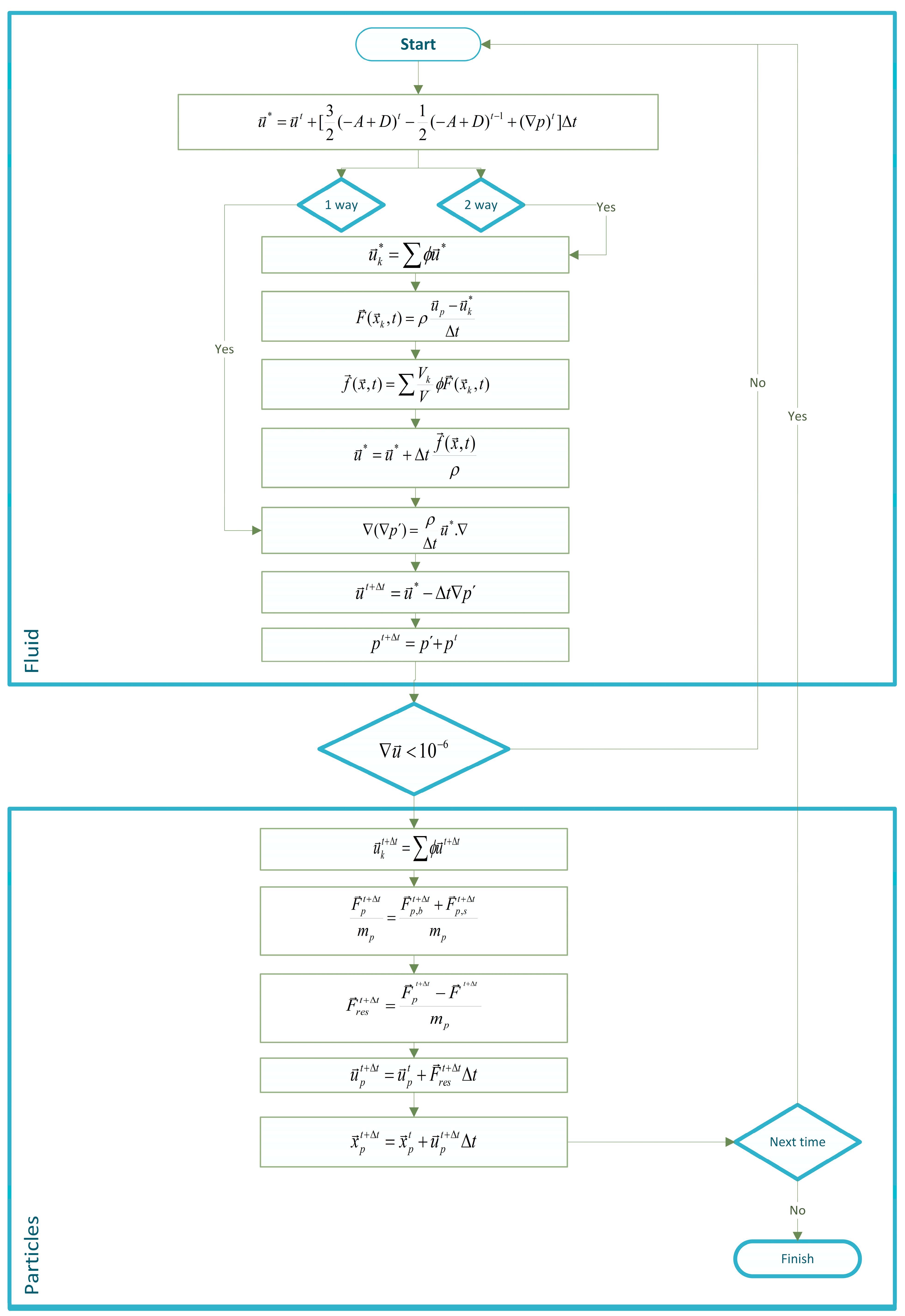
2. Mathematical Model and Numerical Methods

2.1. Fluid Flow Motion Model

The mathematical model used to describe the incompressible and Newtonian fluid, considering constant physical properties throughout space and time, is presented in Equation (1) [20] (mass conservation) and Equation (2) [20] (Navier–Stokes).

$$\nabla .\overrightarrow{u}=0,$$

(1)

$$\frac{\partial \overrightarrow{u}}{\partial t}+\nabla .\left(\overrightarrow{u}\overrightarrow{u}\right)=-\frac{1}{\rho }\nabla p+\nabla .\left[\nu \left(\nabla \overrightarrow{u}+\nabla {\overrightarrow{u}}^T\right)\right]+\frac{\overrightarrow{f}}{\rho },$$

(2)

where $\overrightarrow{u}(\overrightarrow{x},t)$ is the velocity field, $p(\overrightarrow{x},t)$ is the pressure field, $\rho$ is the specific mass and ν is the kinematic viscosity.

The IBM allows for the specification of a particular boundary condition in the fluid flow through the addition of a force field $\overrightarrow{f}(\overrightarrow{x},t)$ which represents any external force acting on the fluid flow. In the present study, this force field is due to the particles immersed in the fluid flow. This source term is calculated in the Lagrangian domain and then transmitted to the Eulerian domain to account for the presence of the particles [13]. The force field $\overrightarrow{f}(\overrightarrow{x},t)$ is null in all Eulerian volumes, except in those neighbouring the Lagrangian markers. Mathematically, the force field is expressed as follows [13]:

$$\overrightarrow{f}\left(\overrightarrow{x},t\right)=\int {\overrightarrow{F}}_k\left(\overrightarrow{x},t\right)\delta \left(\overrightarrow{x}-{\overrightarrow{x}}_k\right)d{x}_k,$$

(3)

where $\delta \left(\overrightarrow{x}-{\overrightarrow{x}}_k\right)$ is a distribution function, $k$ denotes a Lagrangian variable ${\overrightarrow{x}}_k$ is the position of the Lagrangian markers set at the immersed boundary, $\overrightarrow{x}$ is the position of the computational Eulerian mesh and ${\overrightarrow{F}}_k\left(\overrightarrow{x},t\right)$ is the Lagrangian force exerted on the Lagrangian marker ${\overrightarrow{x}}_k$.

Numerically, the Navier–Stokes equations are spatially discretized using the finite volume method, where the spatial derivatives are discretized using the central differencing scheme in a staggered arrangement, as proposed by Patankar [21]. Both advective and diffusive terms are advanced explicitly, using the Adams–Bashforth scheme. The velocity components $u$, $v$ and $w$ are positioned on the volume’s normal faces in the $x$, $y$ and $z$ directions, respectively, whereas scalar values, such as the pressure, are located at the volume’s center. The fractional step method of two steps is employed to deal with the velocity–pressure coupling [22]. From this method, in the predictor step, the velocity field ${\overrightarrow{u}}^{\ast }(\overrightarrow{x},t)$ is calculated by the following:

$$\frac{{\overrightarrow{u}}^{\ast }-{\overrightarrow{u}}^t}{\mathsf{\Delta }t}=\frac{3}{2}(-A+D{)}^t-\frac{1}{2}(-A+D{)}^{t-∆t}-\frac{1}{\rho }\nabla p^t,$$

(4)

where $t$ and $t-∆t$ are an instant in time and a time before the previous instant in time, respectively, $A$ is the net flow of linear momentum by advection and $D$ is the net flow of linear momentum by diffusion. Next, the discretization of the Poisson equation for the pressure fluctuation is expressed by

$$\nabla \left(\nabla p^{\prime }\right)=\frac{\rho }{∆t} {\overrightarrow{u}}^{\ast }.\nabla ,$$

(5)

which leads to a system of algebraic equations which is performed by the packages Epetra, AztecOO and ML, in the Trilinos framework [14]. Then, the corrector step can be performed, in which the velocity field ${\overrightarrow{u}}^{t+∆\mathrm{t}}(\overrightarrow{x},t)$ is obtained as follows:

$$\frac{{\overrightarrow{u}}^{t+∆t}-{\overrightarrow{u}}^{\ast }}{\mathsf{\Delta }t}=-\frac{1}{\rho }\nabla p^{\prime },$$

(6)

which finally leads to the corrected pressure field ${\mathrm{p}}^{t+∆\mathrm{t}}(\overrightarrow{x},t)$:

$$p^{t+∆t}=p^t+p^{\prime },$$

(7)

The numerical solution for the IBM has been described in detail in a previous publication [13]. The method of direct forcing (MDF) was employed to represent the presence of solid boundaries in the fluid flow [11]. The Lagrangian force on the Lagrangian markers ${\overrightarrow{F}}_k\left(\overrightarrow{x},t\right)$, is calculated as follows:

$$\frac{{\overrightarrow{F}}_k\left(\overrightarrow{x},t\right)}{\rho }={\overrightarrow{u}}_p-{\overrightarrow{u}}_k^{\ast },$$

(8)

where ${\overrightarrow{u}}_p$ is the desired velocity at the immersed boundary markers and ${\overrightarrow{u}}_k^{\ast }$ is the interpolated velocity at the Lagrangian marker from the Eulerian field. The moving-least-squares reconstruction method (MLS) is employed to build the transfer functions between the Eulerian and Lagragian mesh [23]. Further details are found in the flowchart shown in Figure 1.

2.2. Particles’ Motion Model

The dispersed phase is treated as a Lagrangian framework, where each particle is considered to be a smooth sphere and the differential equations for calculating the particles’ location, linear and angular velocities in vector form can be written, respectively, as [24]

$$\frac{d{\overrightarrow{x}}_p}{dt}={\overrightarrow{u}}_p,$$

(9)

$$m_p\frac{d{\overrightarrow{u}}_p}{dt}=m_p\frac{3\rho C_D}{4{\rho }_p{d}_p}\left(\overrightarrow{u}-{\overrightarrow{u}}_p\right)\left|\overrightarrow{u}-{\overrightarrow{u}}_p\right|+{\overrightarrow{F}}_{ls}+{\overrightarrow{F}}_{lr}+\left(1-\frac{\rho }{{\rho }_p}\right)m_p\overrightarrow{g},$$

(10)

$$I_p\frac{d{\overrightarrow{\omega }}_p}{dt}={\overrightarrow{T}}_p,$$

(11)

where $m_p$ is the particle mass, $d_p$ is the particle diameter, ${\overrightarrow{x}}_p$ is its position, ${\overrightarrow{u}}_p$ is its velocity, $I_p=0.1 m_p{d}_p^2$ is its moment of inertia, ${\overrightarrow{\omega }}_p$ is its angular velocity, ${\overrightarrow{T}}_p$ is the torque acting on a rotating particle and $\overrightarrow{u}-{\overrightarrow{u}}_p$ is the relative velocity between the phases at the particle’s position. The first term on the right side of Newton’s second law (Equation (10)) is the drag force, the second term is the shear-induced lift force, the third term is the rotation-induced lift force and the last term gathers the terms of the gravity and buoyancy forces. Forces such as Basset and virtual mass have been neglected.

In order to quantify the drag force, the non-dimensional drag coefficient must be defined. The drag coefficient past each particle is evaluated through their correlation [25]:

$$C_D=\frac{24}{{Re}_p}+\frac{2.6({Re}_p/5)}{{\left({Re}_p/5\right)}^{1.52}}+\frac{0.411{({Re}_p/2.63x{10}^5)}^{-7.94}}{1+{({Re}_p/2.63x{10}^5)}^{-8}}+\frac{\mathrm{0,25}({Re}_p/{10}^6)}{1+({Re}_p/{10}^6)},$$

(12)

where the Reynolds number is defined as ${Re}_p=d_p\left|\overrightarrow{u}-{\overrightarrow{u}}_p\right|/\upsilon$, which is based on the particles’/fluid’s relative velocity. Correlation is recommended for use when ${Re}_p<{10}^6$ [25]. The shear-induced lift force is evaluated through [26]

$${\overrightarrow{F}}_{ls}=\frac{\rho }{2}\frac{\pi }{4}{d}_p^3{C}_{ls}[(\overrightarrow{u}-{\overrightarrow{u}}_p)x\overrightarrow{\omega }],$$

(13)

where $\overrightarrow{\omega }$ is the vorticity, ${Re}_s=d_p^2\left|\overrightarrow{\omega }\right|/\upsilon$ is the particle’s Reynolds number for shear flow and $C_{ls}$ represents the ratio of the extended lift force to the Saffman force [27,28]:

$$C_{ls}=\frac{4.1126}{\sqrt{{Re}_s}}[(1-0.3314{\beta }^{0.5})e^{-0.1{Re}_p}+0.3314{\beta }^{0.5}] if {Re}_p\le 40,$$

(14)

$$C_{ls}=\frac{4.1126}{\sqrt{{Re}_s}}[0.0524{(\beta {Re}_p)}^{0.5}] if {Re}_p>40,$$

(15)

where $\beta =0.5{Re}_s/{Re}_p$ for $0.005<\beta <0.4$.

The rotation-induced lift force is evaluated as [29]

$${\overrightarrow{F}}_{lr}=\frac{\rho }{2}\frac{\pi }{4}{d}_p^2{C}_{lr}\left|\overrightarrow{u}-{\overrightarrow{u}}_p\right|\frac{\overrightarrow{\Omega }x(\overrightarrow{u}-{\overrightarrow{u}}_p)}{\left|\overrightarrow{\Omega }\right|},$$

(16)

where the relative rotation is $\overrightarrow{\Omega }=0.5 \nabla x\overrightarrow{u}-{\overrightarrow{\omega }}_p$. The lift coefficient $C_{lr}$ is obtained from the correlation proposed by Oesterlé and Dinh [30], in the range 10 < ${Re}_p$< 140:

$$C_{lr}=0.45+(\frac{{Re}_r}{{Re}_p}-0.45)e^{(-0.05674{{Re}_r}^{0.4}{Re}_p^{0.3})},$$

(17)

with the Reynolds number of particle rotation being ${Re}_r=\rho d_p^2\left|\overrightarrow{\Omega }\right|/\mu$. The torque acting on a rotating particle due to its viscous interaction with the fluid can be computed through

$$T=\frac{\rho d_p^5}{64}{C}_r\left|\overrightarrow{\Omega }\right|\overrightarrow{\Omega },$$

(18)

where $C_r$ is the coefficient of rotation. In case of smaller particle rotation Reynolds numbers, the expression for the $C_r$ is obtained by [31]

$$C_r=\frac{64\pi }{{Re}_r} if {Re}_r\le 32,$$

(19)

while the coefficient for larger particle rotation Reynolds numbers is found to be [32]

$$C_r=\frac{12.9}{{Re}_r^{0.5}}+\frac{128.4}{{Re}_r} if 32<{Re}_r\le 1000.$$

(20)

2.3. Particle–Wall Interactions

The change of the particle’s linear and angular velocities during a wall impact can be obtained from the conservation equations of classical mechanics, assuming infinitesimally short contact times and negligible deformations [33]. The post-collision linear and angular velocities in case of non-sliding are defined as

$${\overrightarrow{u}}_p^{+}={\overrightarrow{u}}_p^{-}-\frac{2}{7}(1+e_t){\overrightarrow{u}}_{pr}^{-}-(1+e_n)({\overrightarrow{u}}_p^{-}.\overrightarrow{n})\overrightarrow{n},$$

(21)

$${\overrightarrow{\omega }}_p^{+}={\overrightarrow{\omega }}_p^{-}+\frac{10}{7}\frac{(1+e_t)}{d_p}\overrightarrow{n}\times {\overrightarrow{u}}_{pr}^{-},$$

(22)

and in case of sliding collision, as

$${\overrightarrow{u}}_p^{+}={\overrightarrow{u}}_p^{-}+(1+e_n)({\overrightarrow{u}}_p^{-}.\overrightarrow{n})\left[{\mu }_{dy}\frac{{\overrightarrow{u}}_{pr}^{-}}{\left|{\overrightarrow{u}}_{pr}^{-}\right|}-\overrightarrow{n}\right],$$

(23)

$${\overrightarrow{\omega }}_p^{+}={\overrightarrow{\omega }}_p^{-}-\frac{5}{d_p}(1+e_n)({\overrightarrow{u}}_p^{-}.\overrightarrow{n})\frac{{\mu }_{dy}}{\left|{\overrightarrow{u}}_{pr}^{-}\right|}\overrightarrow{n}\times {\overrightarrow{u}}_{pr}^{-},$$

(24)

where ${\overrightarrow{u}}_p^{-}$ and ${\overrightarrow{u}}_p^{+}$ are the particle velocities before and after the wall impact. Accordingly, ${\overrightarrow{\omega }}_p^{-}$ and ${\overrightarrow{\omega }}_p^{+}$ are the angular velocities before and after the wall impact. The linear (${\overrightarrow{u}}_p^{-}$) and angular (${\overrightarrow{\omega }}_p^{-}$) velocities of the particles before the collision are known. $e_n$ is the wall’s normal restitution coefficient, $e_t$ is the tangential restitution coefficient, ${\mu }_{st}$ is the static coefficient of friction, $\overrightarrow{n}$ is the normal unit vector pointing outwards from the element face being impacted and ${\overrightarrow{u}}_{pr}$ is the relative velocity at the contact point, given by

$${\overrightarrow{u}}_{pr}={\overrightarrow{u}}_p-({\overrightarrow{u}}_p.\overrightarrow{n})\overrightarrow{n}+\frac{d_p}{2}{\overrightarrow{\omega }}_p\times \overrightarrow{n}.$$

(25)

Considering the present stage of the numerical platform, two coupling approaches between phases are considered: one- and two-way coupling. In a one-way coupled system, the presence of the dispersed phase in the continuous phase is neglected, while, in a two-way coupled system, the dispersed phase is computed into the Navier–Stokes equations through the addition of a force source term. The computational algorithm needed in order to deal with the coupling between phases is described in the flow chart on the following page. The algorithm can be explained in two parts: the fluid flow, and the particle motion solutions.

Considering the fluid flow solution and two-way coupling, an intermediate velocity field ${\overrightarrow{u}}^{\ast }$ without a source term $\overrightarrow{f}$ is computed (Equation (4)). In the next step, ${\overrightarrow{u}}^{\ast }$ is interpolated to the interface through the MLS reconstruction procedure, yielding ${\overrightarrow{u}}_k^{\ast }$. The Lagrangian force $\overrightarrow{F}$ is then determined directly at the surface makers, given by the difference between the desired velocity ${\overrightarrow{u}}_p$ at the interface and the actual velocity ${\overrightarrow{u}}_k^{\ast }$ at the interface, multiplied by the specific mass and divided by the time step $∆t$, with ${\overrightarrow{\mathrm{u}}}_p$ resulting from the equation of the sphere’s motion. Next, $\overrightarrow{F}$ is spread to the Eulerian volumes using an MLS reconstruction method and the resulting Eulerian force $\overrightarrow{f}$ is introduced in the intermediate velocity field ${\overrightarrow{u}}^{\ast }$ [34]. The value of the pressure is obtained from the Poisson equation (Equation (5)), after which the divergence-free velocity field ${\overrightarrow{u}}^{t+∆t}$ (Equation (6)) and the pressure field $p^{t+∆t}$ (Equation (7)) are obtained.

As the fluid flow solution is obtained, the particle motion solution takes place, where the velocity field ${\overrightarrow{u}}^{t+∆t}$ is interpolated to the interface using the MLS method, yielding ${\overrightarrow{u}}_k^{\ast t+∆t}$. In the next step, the sum of drag, shear-induced lift, rotation-induced lift, gravity and buoyancy forces are gathered, yielding ${\overrightarrow{F}}_p^{t+∆t}$. The resulting force action on the particles, ${\overrightarrow{F}}_{res}^{t+∆t}$, is then obtained, which is the difference between the sum of all forces ${\overrightarrow{F}}_p^{t+∆t}$, and the Lagrangian force ${\overrightarrow{F}}^{t+∆t}$. Next, the translation velocity ${\overrightarrow{u}}_p^{t+∆t}$ and position ${\overrightarrow{x}}_p^{t+∆t}$ of the particle are achieved. Furthermore, upon the particle colliding with a wall, the particle’s new linear and angular velocities after rebound are calculated and a new particle position is obtained.

There is no restriction on when the particles may be released into the fluid flow, thus transient phase and steady state can be considered. However, there are some restrictions, as can be seen in the right side of the Newton’s second law equation, which represents the total force exerted by the fluid on the particle. In order to calculate the forces’ terms, the relative velocity between the phases at the sphere position, $\overrightarrow{u}-{\overrightarrow{u}}_p$, is required. The restriction comes from the fact that the velocity $\overrightarrow{\mathrm{u}}$ at the particle’s position is obtained by interpolation (MLS method) of the fluid velocity in the neighboring volumes, in which case an accurate estimate requires that the particle has to be much smaller than the mesh grid.

The time step is obtained by the CFL (Courant–Friedrichs–Lewy) criterion in order to ensure the stability of the methodology, due to the explicit time-marching method employed. The time step calculation is performed by [35]

$$∆t=\mathit{min}\left[1/(\frac{1}{∆t_a}+\frac{1}{∆t_d})\right],$$

(26)

with

$$∆t_a=1/(\overrightarrow{u}/∆\overrightarrow{x}), ∆t_d=1/(2\nu /{∆\overrightarrow{x}}^2),$$

(27)

where $∆t_a$ is the advection limit stability, $∆t_d$ is the diffusion limit stability, $∆\overrightarrow{x}$ is the grid spacing for each direction, and ν is the kinematic viscosity.

In the case of a non-uniform grid, the grid is refined near the walls with an expansion/reduction factor $G$, in accordance with [35,36]

$$∆\overrightarrow{x}=G^{i-1}\left(\frac{1-G}{1-G^{M/2}}\right)\left(\frac{S}{2}\right).$$

(28)

where $∆\overrightarrow{x}$ is the grid spacing for each direction, $M$ is the volume’s number in Cartesian directions and $1\le i\le M/2$.

3. Flow Configuration and Parameters

The fluid flow within a lid-driven cubic cavity containing spherical particles immersed, for an incompressible Newtonian fluid with kinematic viscosity $\mathsf{\nu }$, is considered.

The flow takes place in a cavity of side length $S=0.10$ m, having a depth-to-width aspect ratio and a span-to-width aspect ratio of $1:1$. The lid of the cubic cavity moves parallel to the positive $\mathrm{x}$-axis with steady velocity, where the velocity component $\mathrm{u}$ is set equal to U. No flux and no slip boundary conditions are applied along the other five static faces. The initial condition is zero velocity everywhere, except in the lid.

Two dimensionless numbers can be used to assess the relative influence of viscosity and inertia on the fluid and particle motions, which are the Reynolds and Stokes numbers, respectively. The fluid flow pattern inside the lid-driven cavity depends on the Reynolds number $Re=US/\nu$, while the motion of solid particles suspended in the flow can be characterized by the Stokes number $St={\rho }_p{d_p}^{2}Re/18\rho S^2$, which represents the ratio of the particle’s response time to a characteristic time scale.

Despite its simplicity, the flow in a lid-driven cavity exhibits features of the more complex flow that can possibly occur in incompressible flows such as eddies, secondary flows, complex three-dimensional patterns, chaotic particle motions, instabilities, transition and turbulence. The characteristics and topology of the lid-driven cavity flow depend on the Reynolds number. In the present work, the Re for steady state flow is used.

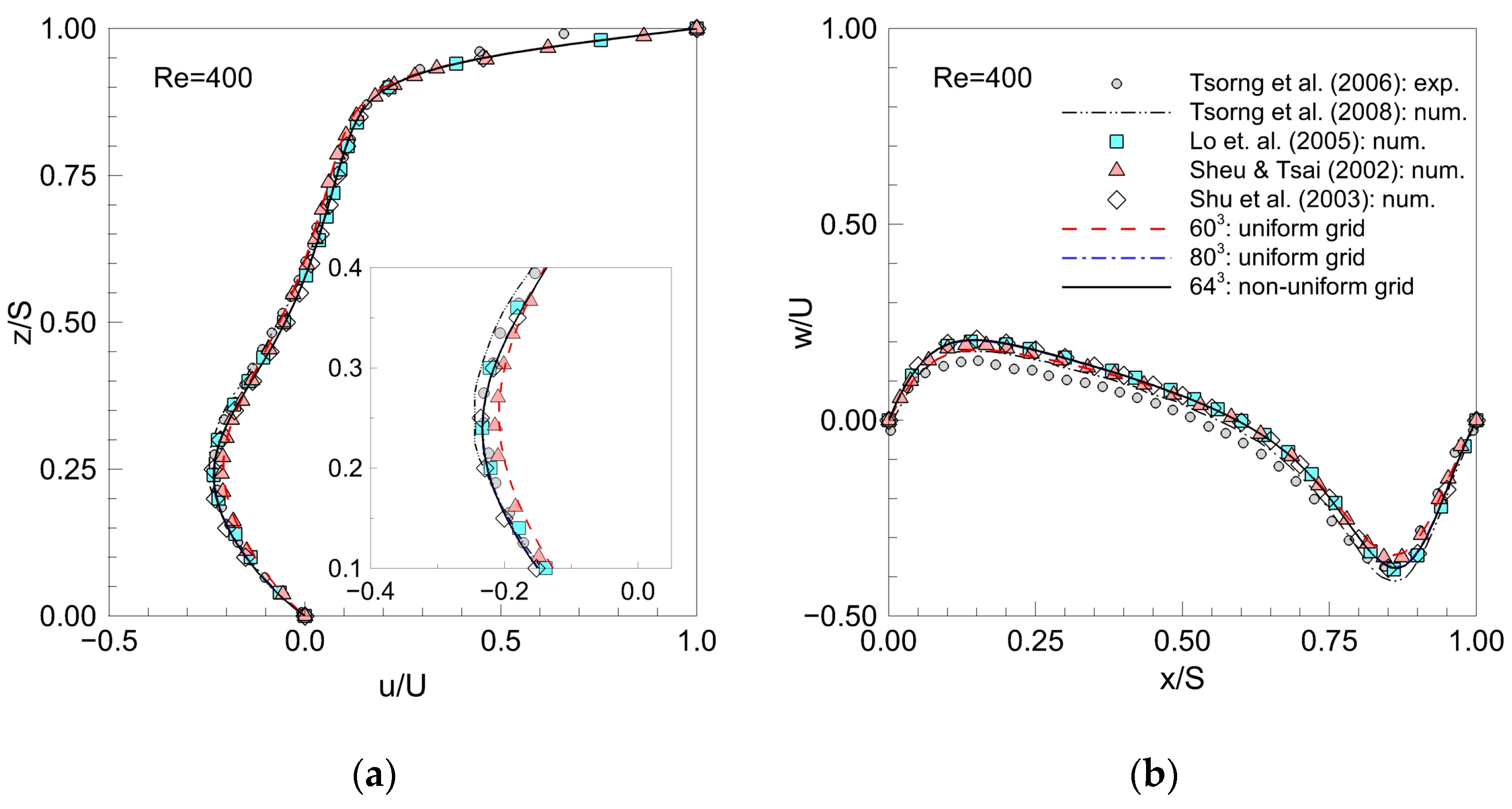
3.1. Validation Process: Lid-Driven Cavity Flow

The reliability of the numerical platform is supported by previously performed verification processes (with manufactured solutions for the pressure field and other expressions for the velocity components and pressure) and validations (incompressible laminar jet, laminar and turbulent lid-driven cavity flows) [14,15]. Based on the proposed problem to be studied, a specific $\mathrm{R}\mathrm{e}$ is considered. The simulations were performed at $\mathrm{R}\mathrm{e}=400$ and $470,\mathrm{c}\mathrm{o}\mathrm{n}\mathrm{s}\mathrm{i}\mathrm{d}\mathrm{e}\mathrm{r}\mathrm{i}\mathrm{n}\mathrm{g}$ uniform grids with ${60}^3$ and ${80}^3$ volumes and a non-uniform mesh with ${64}^3$ volumes where the $∆\mathrm{x}$, $∆\mathrm{y}$ and $∆\mathrm{z}$ have been increased continuously by 2.5% from the cavity wall.

The results were compared with the experimental particle imaging velocimetry measurements [37] and with the numerical results [6,38,39,40]. The results are in good agreement with the referenced data shown in Figure 2, which plots velocity profiles along the vertical and horizontal centerlines of 3D lid-driven cavity. Both profiles showed excellent agreement with Lo et al. [38], who solved the proposed problem using a fine mesh of 101 × 101 × 101 volumes. Since grid-independent solutions are revealed, the uniform mesh of ${80}^3$ volumes has shown similar results to the non-uniform mesh of ${64}^3$ volumes. These results are based on the non-uniform grid due to computational costs.

In order to visualize the 3D flow topology, without considering immersed particles, the streamlines in the selected longitudinal ($\mathrm{x}$-direction) and transverse ($\mathrm{y}$-direction) planes are shown in Figure 3, where the results were compared with the numerical results at a $Re=470$ [6]. The flow pattern is characterized by a large primary eddy, occupying most of the cavity and driven by the moving top lid (red arrow indicates the direction), which can be clearly observed in the longitudinal planes ($y/S=0.5$ and $0.9$). Near the end wall, an inward spiral is associated with suction of the fluid particles towards the core of the primary eddy, known as the spanwise inward current. However, along the cavity’s center plane ($y/S=0.5$), fluid particles spiral outwards, away from the core of the primary eddy and towards the perimeter of the cavity, forming the spanwise outward current. Also, a secondary eddy in the lower downstream corner of the cavity is observed. The center of the primary eddy is located away from the cavity’s center, displaced towards the downstream end wall and the top lid.

In the cavity center’s transverse plane ($x/S=0.5$), the flow has a pattern of symmetric vortices. The vortices bounded by the end walls and the bottom/top walls and are called end-wall vortices (EWVs). The lower part of the EWVs seem to span the width of the cavity, while the upper part of the EWVs do not span the whole width. EWVs are observed on both sides of the cavity, with outward spiral nodes near the bottom, and inward spiral nodes near the top [41]. Considering this particular Reynolds number, Taylor–Görtler-like vortices are not seen in the cavity. The comparison of the left (present) and right (reference [6]) planes of Figure 3 indicates a very good agreement between both simulated results.

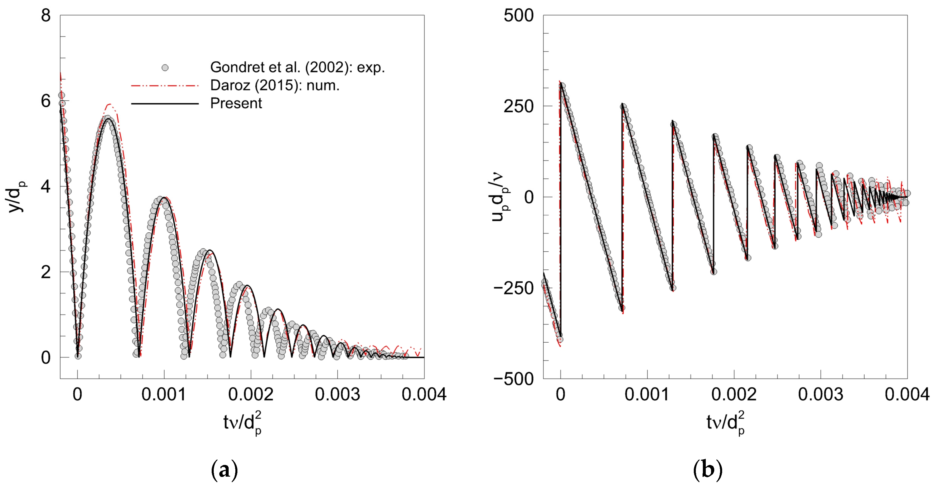
3.2. Validation Process: Bouncing Motion of a Particle–Wall Collision in Fluid

Based on experimental data, the trajectory of a solid sphere falling under gravity in a fluid onto a solid wall is evaluated. The fluid domain is a rectangular vessel with a dimension of $10\times 10\times 30$ cm³. The fluid is still at its initial moment and the spherical particle starts to fall from rest under gravity. The physical properties of the Teflon sphere include a diameter ${\mathrm{d}}_p=6$ mm, density ${\rho }_s=2.15\times {10}^3$ kg/m³, Young’s elastic modulus $E=0.4\times {10}^9$ Pa, Poisson’s ratio $\zeta =0.46$ and a coefficient of restitution $\mathrm{e}=0.80\pm 0.02$ (as if impacting a glass wall in air). The physical properties of air are the specific mass $\mathsf{\rho }=1.2$ kg/m³ and dynamic viscosity $\mu =1.85\times {10}^{-5}$ Pa.s. The Reynolds number and Stokes number at the first impact are, respectively, $Re=210$ and $St=7.8\times {10}^4$ [42].

Figure 4 shows the dimensionless distance of the bottom apex of the sphere to the wall and its instantaneous velocity as a function of dimensionless time. The first collision time was taken as dimensionless time $t\upsilon /{d_p}^2=0$. The rebound trajectories are parabolic and the velocity between collision decreases linearly with time. As kinetic energy is lost due to fluid viscosity and material damping, rebounds become progressively smaller. The present results are in good agreement with experimental [42] and numerical [43] data.

4. Results and Discussion

The numerical simulation of the lid-driven cubic cavity flow with a rigid spherical particle immersed into the flow is now examined. Based on available data from Tsorng et al. [6], the particle has a diameter $d_p=0.003$ m and density ${\rho }_p=1210$ kg/m³, with a relative density $(\rho -{\rho }_p)/\rho \approx 0.05\%$, thus there is a positive buoyancy in which the fluid is slightly heavier than the particle, causing it to rise slowly in the liquid at rest. The kinematic viscosity of the liquid is $\upsilon =3.72\times {10}^{-5}$ ${\mathrm{m}}^2/\mathrm{s}$. The dimensionless numbers $Re=470$ and $St=0.023$ are considered. In order to avoid a start-up transient, the particle is released into the flow at dimensionless time $tU/S=160$.

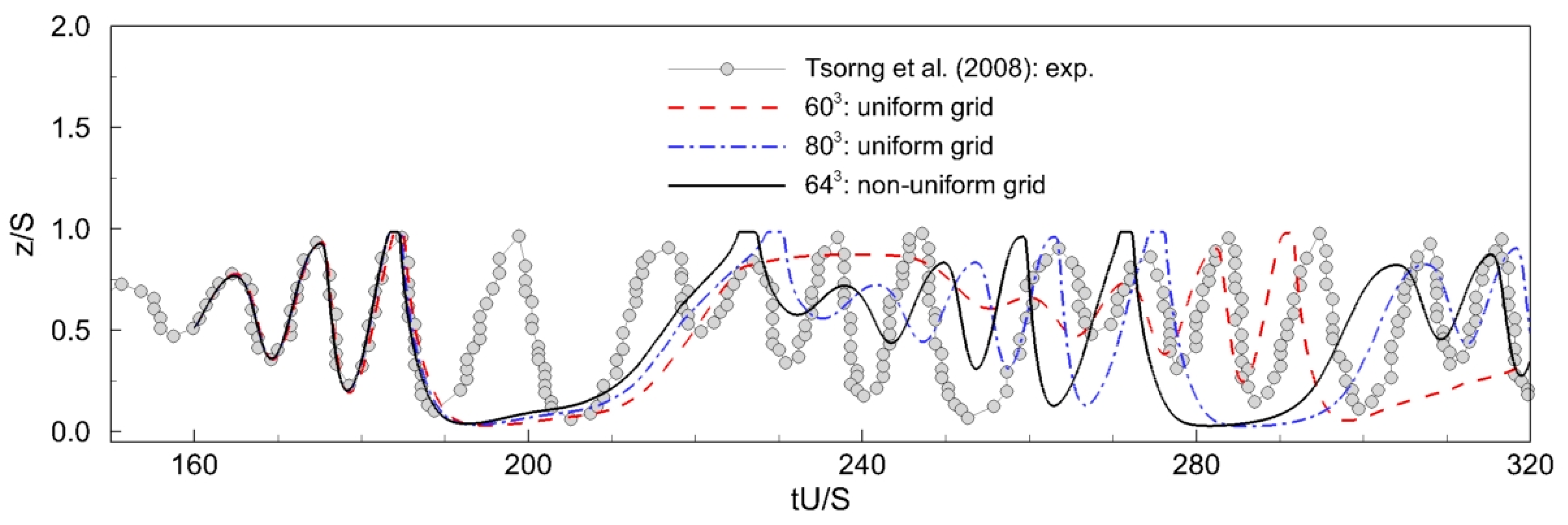
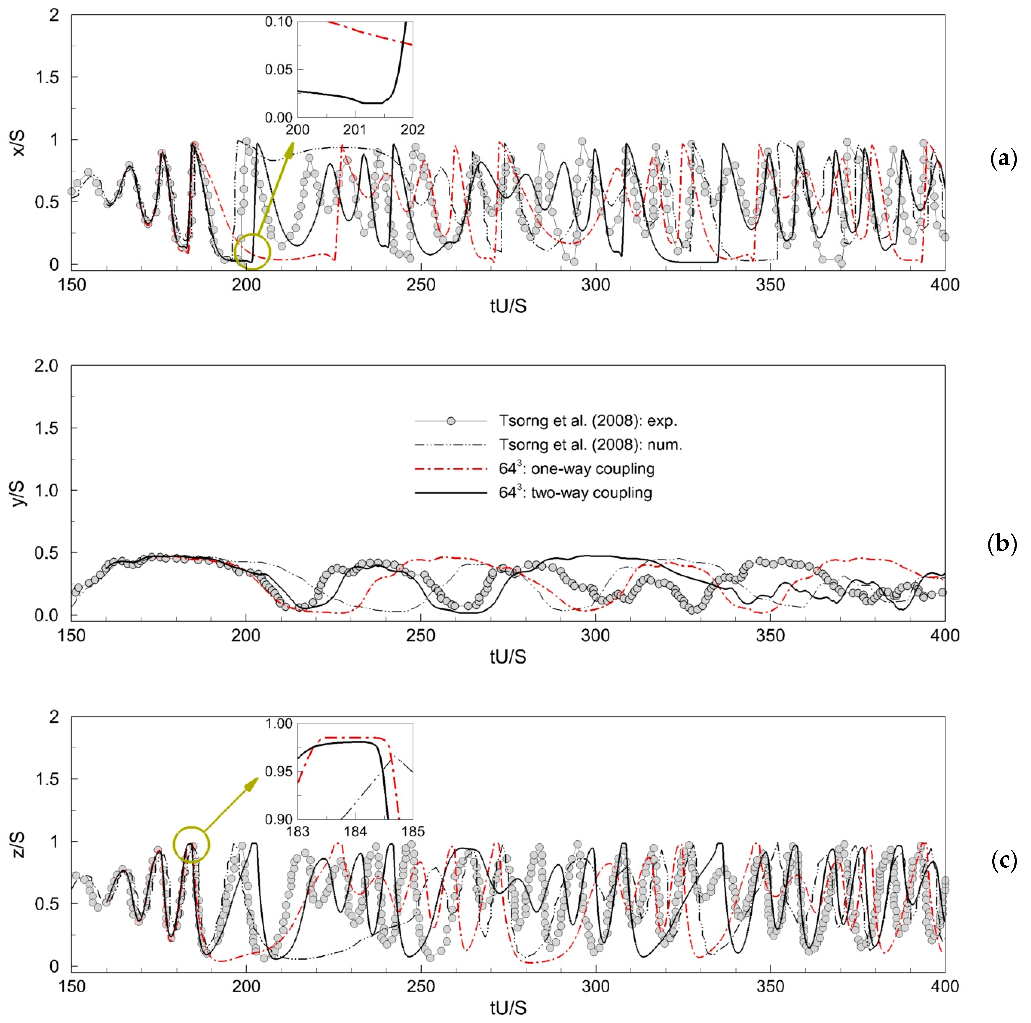
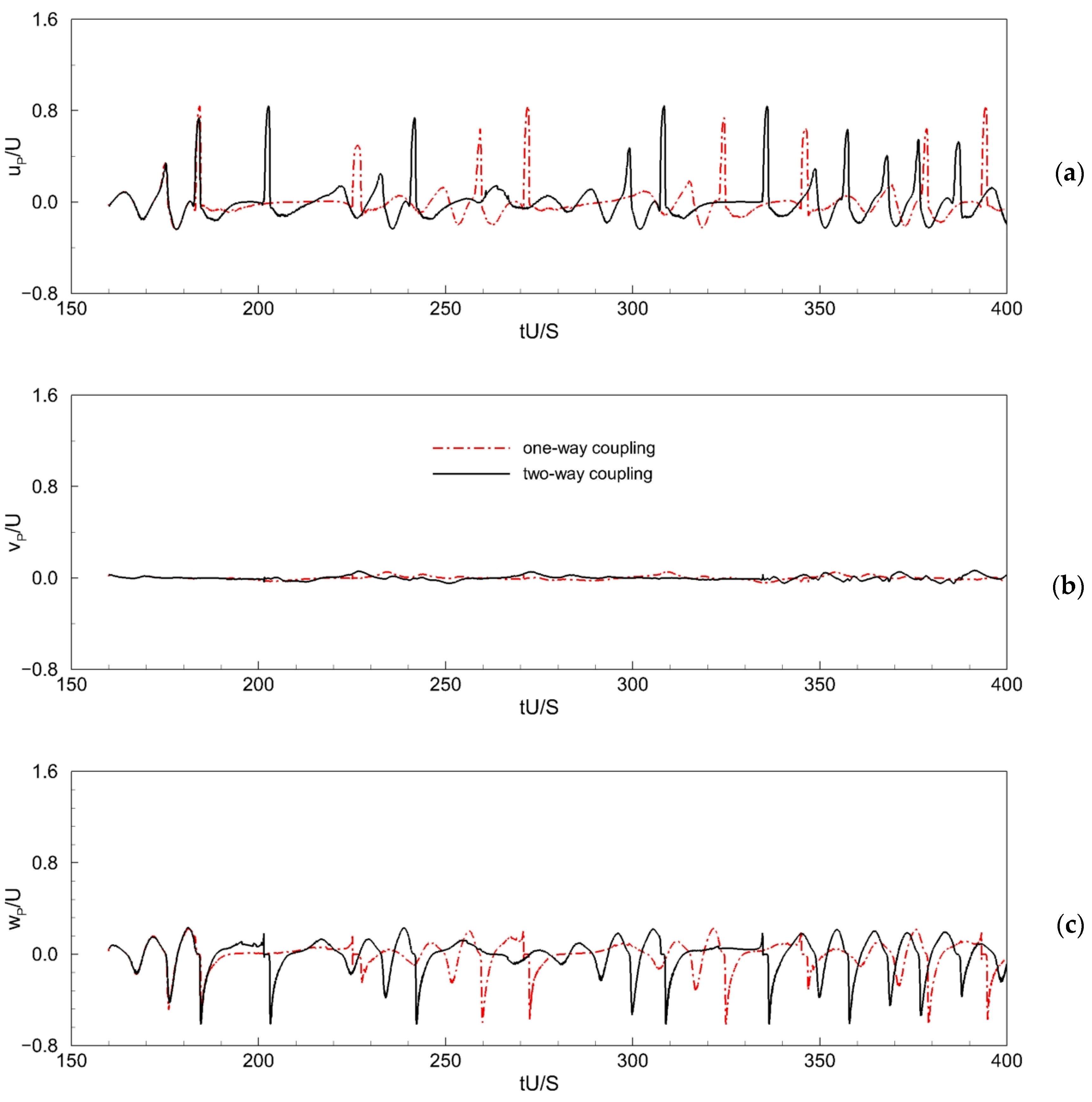
4.1. Three-Dimensional Position Histories and Trajectories of the Particle

Using the same grids employed in the validation process, the complete spatial history of the sphere motion was simulated for each grid (Figure 5). The results of the trajectory in the $\mathrm{z}$ direction come closer to the experimental results as the grid is refined, considering one-way coupling, due to the fact that the velocity gradient is better calculated, mainly in the vicinity of the solid walls. This approach has its limitations, in that the fluid completely influences the motion of the sphere via drag and other forces and the sphere does not affect the fluid flow. Even though the results come closer to the experimental ones as the grid is refined, there is a significant deviation between them. This will be addressed through the application of the two-way coupling approach.

In the work of Tsorng et al. [6], stereoscopic measurements were able to the track particle’s motion throughout the flow and compare the obtained results with numerical ones, where the passive tracers were advected by the flow at the same Reynolds number. These numerical results were obtained by integration of the steady flow field, derived from the Navier–Stokes equations. The particle velocity was assumed to coincide with the local fluid velocity interpolated from the calculated flow field at every single time step, and the simulated path is integrated both forward and back to obtain the complete temporal history of the particle throughout the domain.

A comparison of the experimental and simulated spatial histories over the time interval $160<tU/s<400$ is shown in Figure 6, exhibiting a sequence of repeating irregular cycles where the $\mathrm{x}$ and $\mathrm{z}$ directions are associated with loops inside the cavity (see Figure 7), flowing through currents which make up the first half of the primary eddy.

The particle’s trajectory follows the experimental data until the first collision with a solid surface. In one-way coupling, the spherical particle collides with the top lid ($z/S=1$) around dimensionless time $tU/S=183$ (beginning of the horizontal plateau of the red dash-dotted line, as shown in the inset of Figure 6c), while for the two-way coupling it occurs first with the backward wall ($x/S=0$) in the upper half, and then with the top lid, around dimensionless time $tU/S=201$ (beginning of the horizontal plateau of the black solid line, as shown in the inset of Figure 6a). After this first contact, there is a deviation between the results, however, the two-way coupling results better approximate the experimental data, followed by the one-way coupling and then the passive tracer.

In the $\mathrm{y}$ direction, the particle is first carried by the spanwise outward current to the near-wall region ($y/S=0$), and then the particle is carried by the spanwise inward current from the near-wall region towards the center plane ($y/S=0.5$). From the simulated time interval, three cycles can be clearly seen in Figure 6b, where the particle spends more time near the centre plane than the near-wall region. In the one-way coupling, the particle reaches the most extreme layers with the spanwise outward current, getting close to the cavity bottom, where the velocities are lower. This is the reason why it takes longer to move near this region, forming a plateau. The same observation is reported for the numerical solution of the reference using the passive tracer, which however, happens on a different layer.

Although the two-way approach better represented the experimental data, there is a slight discrepancy from the first collision, which may be associated with the empirical coefficients employed in the collision model.

Figure 8 shows the dimensionless velocity components of the particle throughout dimensionless time, which is directly associated with its position in the cavity. Due to the loop around the primary eddy, in the top lid region, the sphere reaches a maximum velocity of $u_p=0.84U$ many times, for both couplings between phases. There is a quick sphere translation in this region due to the imposed top lid velocity $U$, which can be seen in the dimensionless velocity in Figure 8a. As the particle comes closer to the frontal top lid border, the particle decelerates in the $x$ direction, and starts its downward translation in the $\mathrm{z}$ direction, accelerating and reaching higher negative velocity of $w_p=-0.61U$ for both couplings between phases (Figure 8c). Next, the particle continues to loop around the primary eddy, decelerating in the $z$ direction and accelerating in the $\mathrm{x}$ direction, limited by the secondary eddy, reaching a minimum velocity of $u_p=-0.24U$ (Figure 8a). The particle remains in this region for a prolonged period of time when compared to its time in the top lid region. In order to complete the cycle, the particle decelerates in the $x$ direction and accelerates in the $z$ direction, reaching a maximum speed of $w_p=0.23U$. In the $y$ component, the particle makes its way from the wall to the cavity center and back again. Since the flow is not preferential in this direction, the particle velocity displays low values.

Three-dimensional views of the associated particle trajectories are presented in Figure 7. The spherical particle stays confined to a single side of the cavity, which is associated with the steady state flow once the flow is symmetric in relation to the median plane ($y/S=0.5$). When comparing the present results, the sphere continues to loop around the primary eddy. This same behavior is obtained experimentally [6]. However, the simulated results [6] show that the tracer passes from the primary to the corner eddy along the downstream end wall, slowly drifts towards the sidewall, and then turns back to the primary eddy, which is highlighted in gray (Figure 7d), between the dimensionless times $tU/S=200$ and $250$. When comparing both couplings between phases, the particle reaches the most extreme layers of the spanwise outward current for the one-way coupling between the dimensionless times $tU/S=200$ and $210$. The particle remains near the cavity bottom for longer until it continues to loop around the primary eddy. The same behavior with less intensity can be seen in this region, between the dimensionless times $tU/S=285$ and $292$. From the dimensionless velocity (Figure 8) components, it is clearly observed that the very slow particle motion in this region induces a small displacement in a large time interval (Figure 6).

As expected, the two-way coupling simulation has better represented the dynamics of the particle inside the cavity. The presence of the particle in the continuous phase affects the momentum locally, leading to a lower acceleration when compared to the one-way coupling. This fact causes all the differences pointed out in the analysis of the present results and in the quantification of the associated forces.

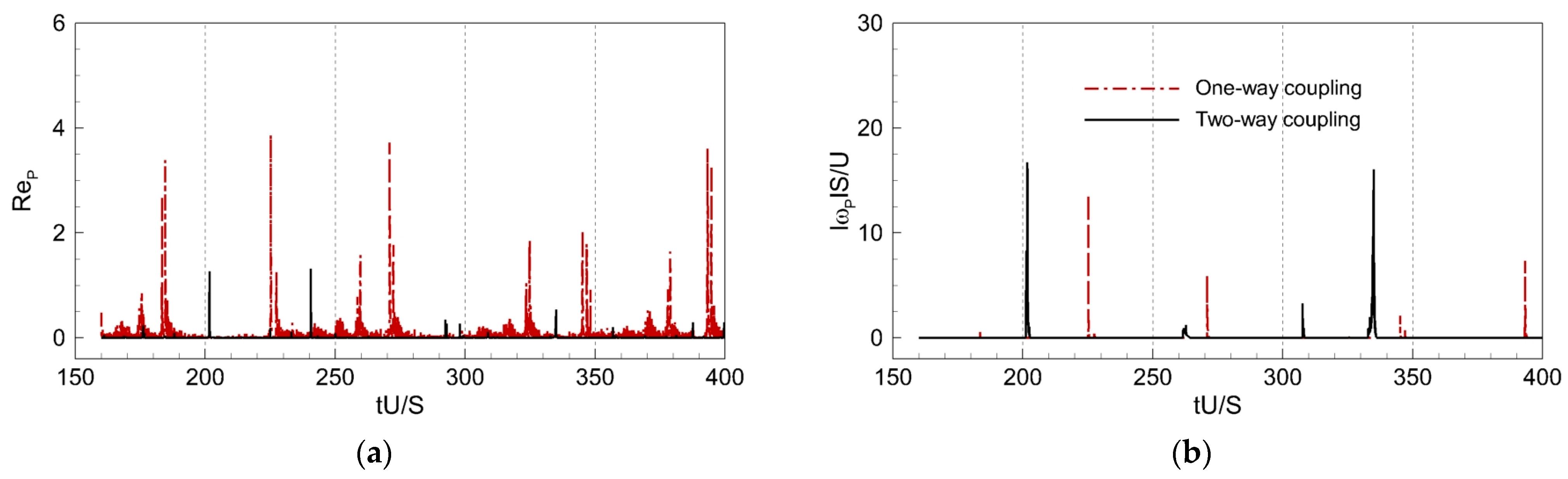
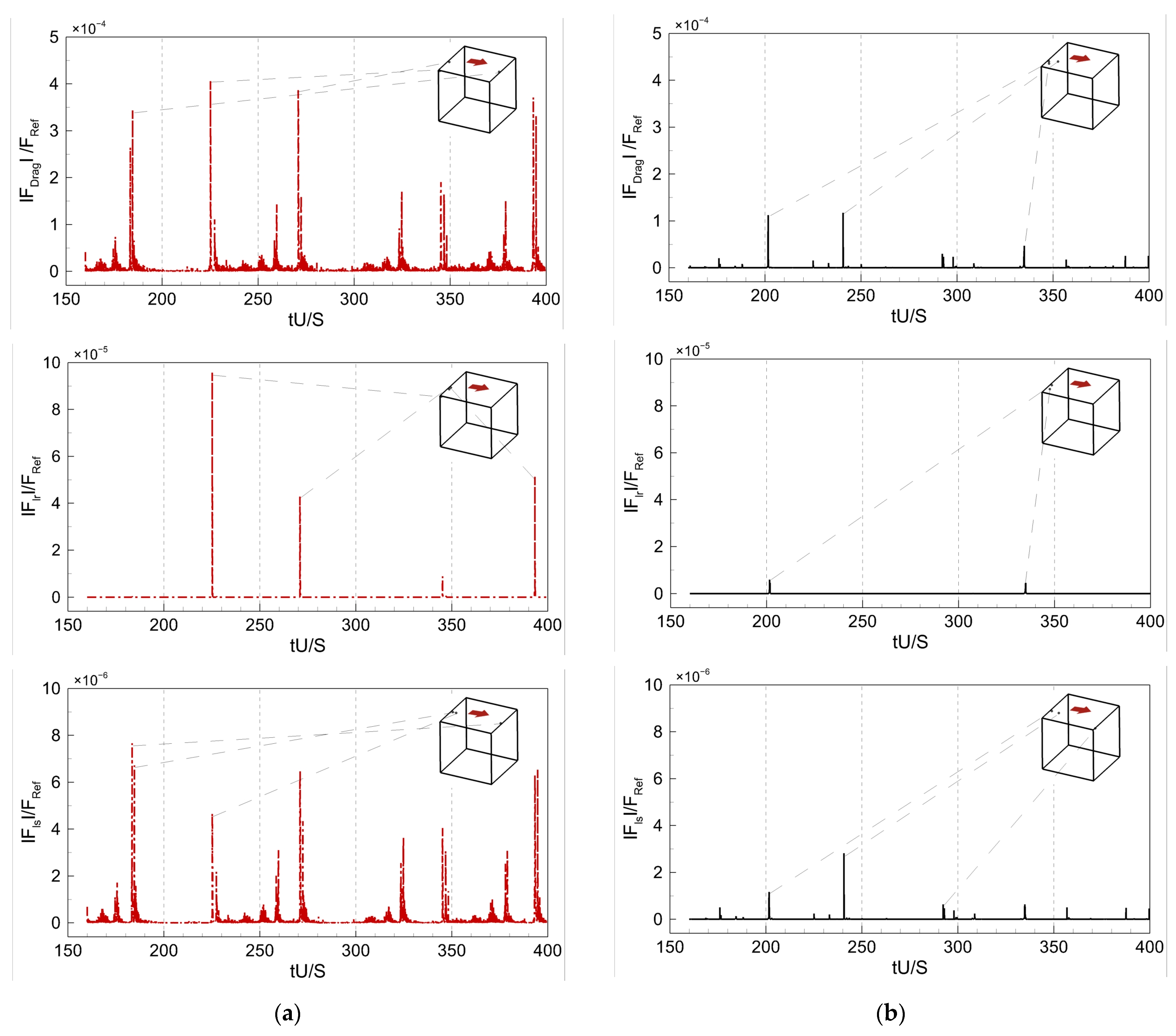
4.2. Forces Acting on the Particle

When dealing with the particle’s motion, the relative velocity between the phases at the sphere position, $\overrightarrow{u}-{\overrightarrow{u}}_p$, has the important role of influencing the ${Re}_p$ and the forces acting on the particle. The velocity $\overrightarrow{u}$ at the particle’s position is obtained by interpolation of the fluid velocity in the neighboring volumes, while ${\overrightarrow{u}}_p$ is the particle’s velocity. The relative velocity shows higher values when the particle collides with the top lid region, and its magnitude is higher for the one-way coupling than the two-way coupling. As the particle approaches the top lid, there is a rapid acceleration of the particle. Once the top lid has an imposed its velocity $U$, this momentarily leads to a higher relative velocity, as represented by the peaks. The wall–particle collisions with the top lid lead to higher values of the relative velocity and, consequently, a higher ${Re}_p$ (Figure 9a). Also, particle–wall collisions induce particle rotations, which can be seen in the higher values of the normalized particle rotation magnitude $\left|{\omega }_p\right|S/U$ (Figure 9b).

Figure 10 shows the drag, shear-induced lift and rotation-induced lift forces which have been normalized with the reference force $F_{ref}=\rho U^2{S}^2/2$. The dimensionless force peaks are associated with the relative velocity of the particle near the wall–particle collision position (as identified in Figure 10). In terms of the rotation magnitude, in general, the drag force has demonstrated a higher influence on the sphere’s motion, followed by the rotation-induced lift force and shear-induced lift force.

An examination of the first collision with the top lid, for one-way coupling, shows that around dimensionless time $tU/S=183,$ the magnitude of the drag force is 34 times higher than the shear-induced lift force and that a very low value of the rotation-induced lift force is present. The shear-induced lift force is associated with the velocity gradient near the wall, while the rotation-induced lift force is associated with the particle’s rotation. On the other hand, in the first collision of the two-way coupling simulation, the drag force is 96 times higher than the shear-induced lift force and 19 times higher than the rotation-induced lift force when the particle collides first with the backward wall ($x/S=0$) and then with the top lid ($z/S=1$), around dimensionless time $tU/S=201$.

In the second particle–wall collision, for the one-way coupling, a higher value of the drag force is achieved, which is associated with a higher relative velocity and higher ${\mathrm{R}\mathrm{e}}_{\mathrm{p}}$ (Figure 9a). Unlike the first collision, this time the collision with the top lid induces significant particle rotation (Figure 9b), achieving higher values of rotation-induced lift force, around dimensionless time $tU/S=225$. The drag force is 87 times higher than the shear-induced lift force and 4 times higher than the rotation-induced lift force. Around dimensionless time $tU/S=240$, for the two-way coupling, the particle achieved a position very close to the top lid without colliding with the wall. In this case, the drag force is 42 times higher than the shear-induced lift force and the rotation-induced lift force is neglected.

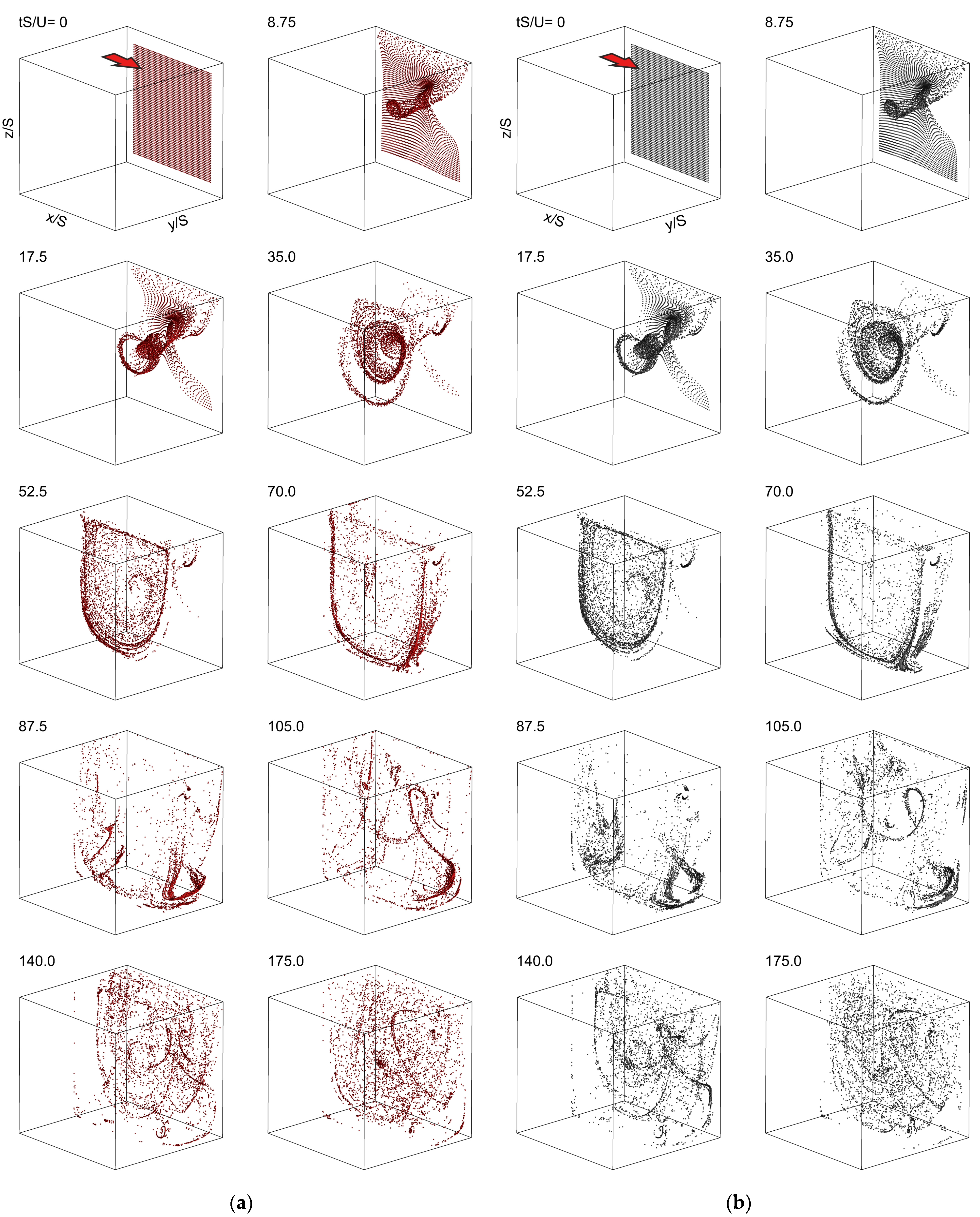
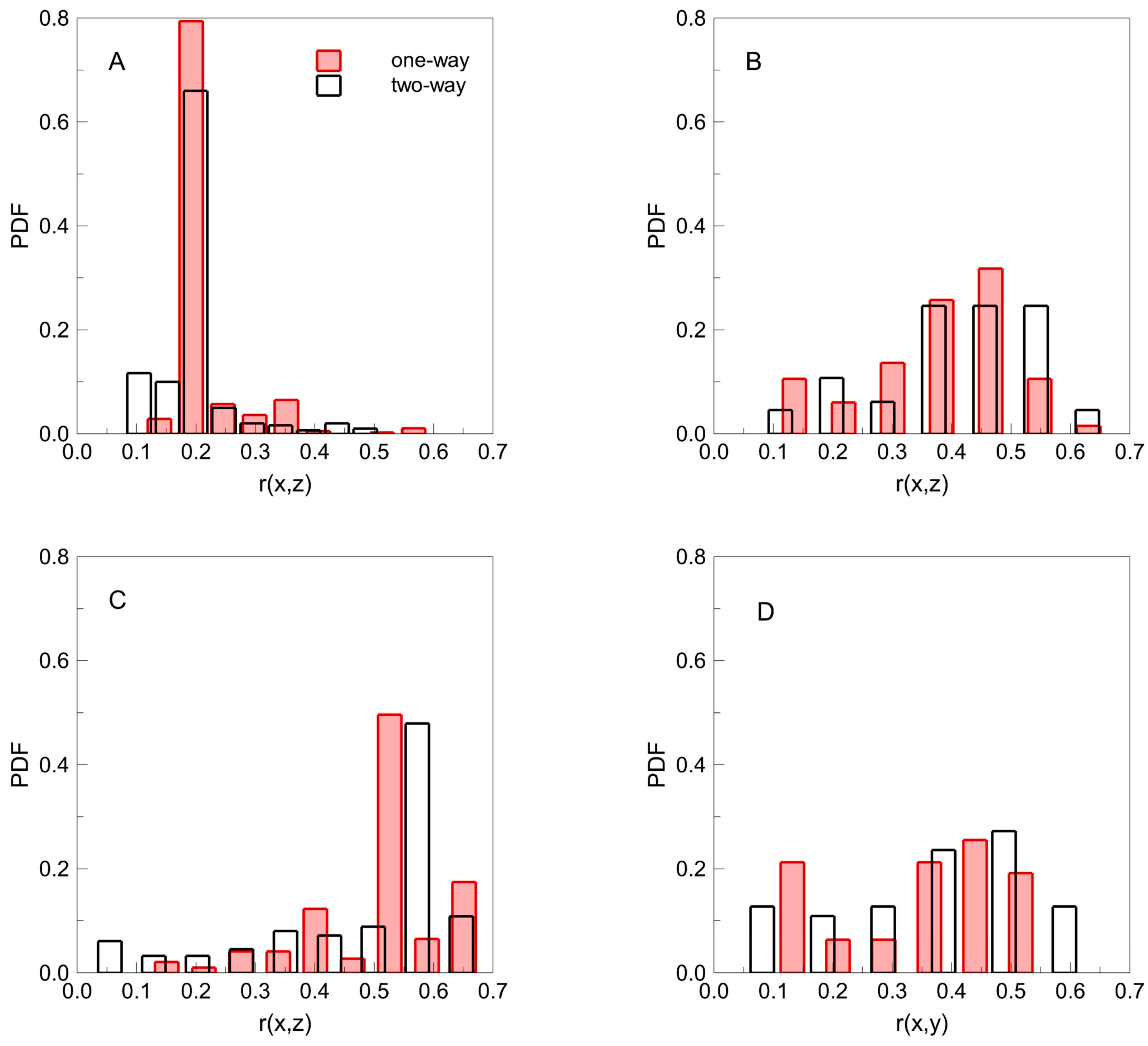
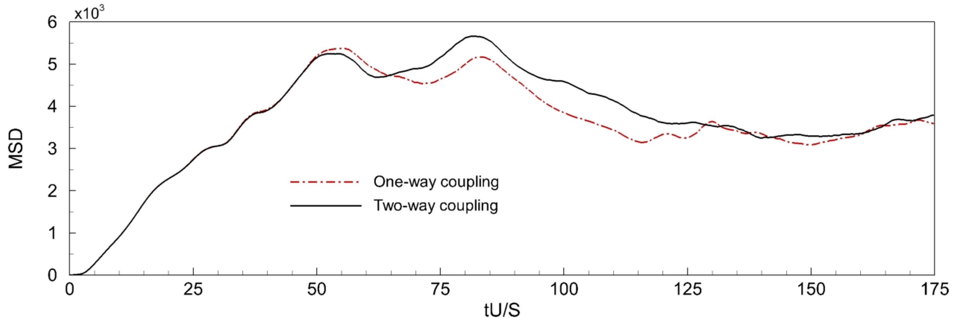
4.3. Simulation of Proposed Problem with 4225 Particles

Once a single spherical particle’s motion had been examined, 4225 particles were included in the fluid flow, the latter being uniformly distributed on the plane $y/S=0.975$, as shown in Figure 11. The volume fraction of the particles is ${\mathsf{\Phi }}_{\mathrm{p}}=0.0011$. Initially, both the fluid and the particles are at rest. In order to deal with the higher number of particles and considering the rate of $L_c/d_p=1.5625$ (where $L_c$ is the distance between the particles’ centre), particles with a smaller diameter $d_p=8.0\times {10}^{-4} m$ are employed, leading to $St=0.00167$. Also, a $Re=470$ is considered. As recommended in the case of many particles immersed in the fluid flow, the particles’ diameter employed in the simulations is smaller than the mesh grid [44]. The normal and tangential restitution coefficients are 0.8 and 1.0, respectively. Also, the static and dynamic friction coefficients are, respectively, 0.9 and 0.5 for the particle–wall collision modeling.

The particle dynamics throughout dimensionless time is shown in Figure 11, where both couplings between phases exhibit similar qualitative behaviors, with their concentrations’ variation observed in certain regions. The particles start from close to the end wall ($tU/S=0$), after which the particles are conducted into the primary core through the spanwise inward current, spiraling along the central axis of the cavity towards the center of the plane ($tU/S=8.75$ and $17.5$). Along the cavity median plane, fluid particles spiral outwards, away from the core of the primary eddy ($tU/S=35.0$ and $52.5$), with most particles reaching the spanwise outward current. The particles that reach the upper downstream corner ($tU/S=70.0$) proceed through a narrow corridor down the end wall until they reach the secondary eddy (as indicated in Figure 11a,b) in the lower downstream corner ($tU/S=87.5$ and $105.0$). When the particles approach the end wall, the cycle starts again, directing them to the spanwise inward current and occupying half of the cavity.

Figure 12 shows the spatial distribution of the particles in planes A–D (detailed in

Table 1. Planes’ position and their number of particles.

Plane	Position	Number of Particles	Fraction of Particles (%)
A	y/S = 0.994	300	7.10
B	y/S = 0.750	65	1.54
C	y/S = 0.501	461	10.91
D	z/S = 0.500	55	1.30

) and the statistical analysis of these planes. These Cartesian planes show the particles’ positions at dimensionless time $tU/S=175.0$ in the two-way coupling simulation. The particles’ positions were converted into a radial position $r$. A histogram from all the calculated radial positions $r$ on the planes, when normalized, yields the probability density function (PDF) which indicates the probability of a particle being located at radius $r$ [45]. Figure 12b shows the PDF extracted from the referred planes.

The number of particles contained in the referred planes and that fraction in relation to the total number of particles are also shown in Table 1. The number of particles in the planes ranges from 55 to 461 particles, which correspond to 1.30% and 10.91% of the total number of particles, respectively. The largest number of particles are in plane C, while the smallest number of particles are in plane D for this specific instant of dimensionless time.

The histogram corresponding to plane A shows the high probability of particles being close to $r=0.2$ ($PDF=0.66$), where the particles are drawn inwards into the primary vortex. In plane B, there is a range of $r=0.35-0.55$ ($PDF=0.25$), with evidence showing that 75% of particles in this plane are concentrated in this spatial interval. The higher value of PDF for the plane C is near $r=0.6$ ($PDF=0.48$), which includes the corresponding entrance region of the secondary vortex. In plane D, the particles are better distributed when compared to the other planes.

When comparing the probability density function of both couplings between phases at the same dimensionless time, they show similar distribution patterns for the referred planes. The differences found between them are shown in Figure 13. When considering the places of high concentration, higher values of $PDF$ are found for the one-way coupling when compared to the two-way coupling, except in plane D. In general, the distribution difference in the histograms must be in agreement with the relative percentage difference (relative to the two-way coupling) of the total number of particles found in the four planes. With 881 particles in the four planes for the two-way coupling, the relative difference between the coupling phases is 10.44%.

In order to better quantify the dynamics of the particles, the following statistical analysis is performed using the so-called mean square displacement (MSD) method:

$$MSD(t)=\frac{1}{N}\sum [{(x_{ki}(t)-x_{k0i})}^2+{(y_{ki}(t)-y_{k0i})}^2+{(z_{ki}(t)-z_{k0i})}^2],$$

(29)

where, $x_{ki}, y_{ki}, z_{ki}$ is the particle’s position at the dimensionless time $tU/S$, $x_{k0i}, y_{k0i}, z_{k0i}$ is the particle’s initial position and $N$ is the number of particles. This expression allows us to quantify the dispersion of the particles [46].

The variation of the mean square displacement for both couplings between phases is shown in Figure 14. Over the sub-interval $0<tU/S<47.2$, both results are in rather close agreement. In this interval, most of the particles reach the median plane (see Figure 11). Going forward in time, there is a deviation between them. The maximum MSD values for each simulation are given at different dimensionless times. From $tU/S=130.0$, the mean square displacement oscillates around the same value for both cases, indicating little variation in the particles’ distribution within the cavity, and good agreement between them. The variation observed in the last instant of the dimensionless time ($tU/S=175.0$) and is reflected in specific planes that are shown in Figure 13.

5. Conclusions

In the present work, the immersed boundary method and the Euler–Lagrange approach have been employed in the case of a lid-driven cavity flow to represent confined flow, in order to numerically predict three-dimensional particle motion by considering nearly neutrally buoyant conditions. Drag and lift forces, particle rotation, particle–wall interactions and the coupling between phases (one- and two-way coupling) have been considered.

Despite its simplicity, the flow in a lid-driven cavity exhibits features of a complex flow. The flow pattern is characterized by a large primary eddy, occupying most of the cavity and driven by the moving top lid. Near the end wall, an inward spiral is associated with suction of the fluid particles towards the core of the primary eddy. Along the cavity center plane, fluid particles spiral outwards, away from the core of the primary eddy and towards the perimeter of the cavity. Additionally, a secondary eddy in the lower downstream corner of the cavity is observed. Based on simulations with a $Re=470$, the flow is symmetric with respect to the median plane.

When dealing with a single spherical particle immersed into the fluid flow, the particle is released at a steady state flow. A comparison of the experimental and simulated spatial histories was performed, where the particle trajectory follows the experimental data until the first collision with a solid surface. After this first contact, there is a deviation between the results, however, the two-way coupling results are in better agreement with the experimental data, when compared to the one-way coupling results. The peaks of the dimensionless forces acting on the particles are associated with the relative velocity of the particles near the wall–particle collision position. In terms of magnitude, in general, the drag force has shown a higher influence on the sphere’s motion, followed by the rotation-induced lift and shear-induced lift forces.

A simulation with 4225 particles, uniformly distributed on the plane $\mathrm{y}/\mathrm{S}=0.975$, released at the beginning of the flow, which corresponds to a volume fraction of approximately $0.11$%, was also evaluated. The particle dynamics throughout dimensionless time has shown similar behaviour for both couplings between phases, with variations in local concentrations observed in certain regions. The probability density function which indicates the probability of a particle being located at a specific position was also evaluated for different planes, showing that the particles’ concentration is associated with the inward/outward spiral into the primary vortex. The mean square displacement used to quantify the dispersion evolution of the particles showed that the particulate flow reaches an approximately homogeneous distribution from the moment of dimensionless time $tU/S=130.0$.

The work presented in this research paper has shown its reliability in reproducing the physics of the problem, showing a very good agreement with experimental data. Although it has limitations, such as high values of the particle volume fraction and particle–particle interaction, the numerical platform can be confidently used for the analysis of particulate systems in complex flows (pollutant dispersion and downhole flow with particles).

References

1. Augusto, L.L.X.; Lopes, G.C.; Gonçalves, J.A.S. A CFD Study of Deposition of Pharmaceutical Aerosols under Different Respiratory Conditions. Braz. J. Chem. Eng. 2016, 33, 549–558. [Google Scholar] [CrossRef]
2. De Souza, F.J.; Salvo, R.D.V.; Martins, D.D.M. Simulation of the Performance of Small Cyclone Separators through the Use of Post Cyclones (PoC) and Annular Overflow Ducts. Sep. Purif. Technol. 2015, 142, 71–82. [Google Scholar] [CrossRef]
3. dos Santos, V.F.; de Souza, F.J.; Duarte, C.A.R. Reducing Bend Erosion with a Twisted Tape Insert. Powder Technol. 2016, 301, 889–910. [Google Scholar] [CrossRef]
4. Moslemi, A.; Ahmadi, G. Study of the Hydraulic Performance of Drill Bits Using a Computational Particle-Tracking Method. SPE Drill. Complet. 2014, 29, 28–35. [Google Scholar] [CrossRef]
5. Jadhav, A.J.; Barigou, M. Eulerian-Lagrangian Modelling of Turbulent Two-Phase Particle-Liquid Flow in a Stirred Vessel: CFD and Experiments Compared. Int. J. Multiph. Flow 2022, 155, 104191. [Google Scholar] [CrossRef]
6. Tsorng, S.J.; Capart, H.; Lo, D.C.; Lai, J.S.; Young, D.L. Behaviour of Macroscopic Rigid Spheres in Lid-Driven Cavity Flow. Int. J. Multiph. Flow 2008, 34, 76–101. [Google Scholar] [CrossRef]
7. Elghobashi, S. On Predicting Particle-Laden Turbulent Flows. Appl. Sci. Res. 1994, 52, 309–329. [Google Scholar] [CrossRef]
8. Greifzu, F.; Kratzsch, C.; Forgber, T.; Lindner, F.; Schwarze, R. Assessment of Particle-Tracking Models for Dispersed Particle-Laden Flows Implemented in OpenFOAM and ANSYS FLUENT. Eng. Appl. Comput. Fluid Mech. 2016, 10, 30–43. [Google Scholar] [CrossRef]
9. Peskin, C.S. Flow Patterns around Heart Valves: A Numerical Method. J. Comput. Phys. 1972, 10, 252–271. [Google Scholar] [CrossRef]
10. Lima, E.; Silva, A.L.F.; Silveira-Neto, A.; Damasceno, J.J.R. Numerical Simulation of Two-Dimensional Flows over a Circular Cylinder Using the Immersed Boundary Method. JCoPh 2003, 189, 351–370. [Google Scholar] [CrossRef]
11. Uhlmann, M. An Immersed Boundary Method with Direct Forcing for the Simulation of Particulate Flows. J. Comput. Phys. 2005, 209, 448–476. [Google Scholar] [CrossRef]
12. Wang, Z.; Fan, J.; Luo, K. Combined Multi-Direct Forcing and Immersed Boundary Method for Simulating Flows with Moving Particles. Int. J. Multiph. Flow 2009, 34, 283–302. [Google Scholar] [CrossRef]
13. Borges, J.E.; Lourenço, M.; Padilla, E.L.M.; Micallef, C. Immersed Boundary Method Application as a Way to Deal with the Three-Dimensional Sudden Contraction. Computation 2018, 6, 50. [Google Scholar] [CrossRef]
14. Borges, J.E.; Padilla, E.L.M.; Lourenço, M.A.S.; Micallef, C. Large-Eddy Simulation of Downhole Flow: The Effects of Flow and Rotation Rates. Can. J. Chem. Eng. 2021, 99, S751–S770. [Google Scholar] [CrossRef]
15. de Souza Lourenço, M.A.; Padilla, E.L.M. An Octree Structured Finite Volume Based Solver. Appl. Math. Comput. 2020, 365, 124721. [Google Scholar] [CrossRef]
16. Nascimento, A.A.; Mariano, F.P.; Padilla, E.L.M.; Silveira-Neto, A. Comparison of the Convergence Rates between Fourier Pseudo-Spectral and Finite Volume Method Using Taylor-Green Vortex Problem. J. Braz. Soc. Mech. Sci. Eng. 2020, 42, 491. [Google Scholar] [CrossRef]
17. Borges, J.E.; de Souza Lourenço, M.A.; Padilla, E.L.M.; Micallef, C. A Simplified Model for Fluid–Structure Interaction: A Cylinder Tethered by Springs in a Lid-Driven Cavity Flow. J. Braz. Soc. Mech. Sci. Eng. 2021, 43, 504. [Google Scholar] [CrossRef]
18. Borges, J.E.; Padilla, E.L.M. Influence of Forced Oscillation, Orbital Motion, Axial Flow and Free Motion of the Inner Pipe on Taylor–Couette Flow. J. Braz. Soc. Mech. Sci. Eng. 2021, 43, 85. [Google Scholar] [CrossRef]
19. Monteiro, L.M.; Mariano, F.P. Flow Modeling over Airfoils and Vertical Axis Wind Turbines Using Fourier Pseudo-Spectral Method and Coupled Immersed Boundary Method. Axioms 2023, 12, 212. [Google Scholar] [CrossRef]
20. White, F.M. Viscous Fluid Flow, 3rd ed.; McGraw-Hill Series in Mechanical Engineering; McGraw-Hill: Boston, MA, USA, 2006; ISBN 978-0-07-240231-5. [Google Scholar]
21. Patankar, S.V. Numerical Heat Transfer and Fluid Flow, 1st ed.; CRC Press: Boca Raton, FL, USA, 2018; ISBN 978-1-315-27513-0. [Google Scholar]
22. Kim, J.; Moin, P. Application of a Fractional-Step Method to Incompressible Navier-Stokes Equations. J. Comput. Phys. 1985, 59, 308–323. [Google Scholar] [CrossRef]
23. Vanella, M.; Balaras, E. A Moving-Least-Squares Reconstruction for Embedded-Boundary Formulations. J. Comput. Phys. 2009, 228, 6617–6628. [Google Scholar] [CrossRef]
24. Bodnár, T.; Galdi, G.P.; Nečasová, Š. (Eds.) Particles in Flows, 1st ed.; Advances in Mathematical Fluid Mechanics; Birkhäuser: Cham, Switzerland, 2017; ISBN 978-3-319-60282-0. [Google Scholar]
25. Morrison, F.A. An Introduction to Fluid Mechanics, 1st ed.; Cambridge University Press: Cambridge, UK, 2013; ISBN 978-1-139-04746-3. [Google Scholar]
26. Sommerfeld, M. Theoretical and Experimental Modelling of Particulate Flows. Available online: https://www.yumpu.com/en/document/view/18701972/theoretical-and-experimental-modelling-of-particulate-flows (accessed on 20 November 2023).
27. Saffman, P.G. The Lift on a Small Sphere in a Slow Shear Flow. J. Fluid. Mech. 1965, 22, 385–400. [Google Scholar] [CrossRef]
28. Mei, R. An Approximate Expression for the Shear Lift Force on a Spherical Particle at Finite Reynolds Number. Int. J. Multiph. Flow 1992, 18, 145–147. [Google Scholar] [CrossRef]
29. Crowe, C.T.; Schwarzkopf, J.D.; Sommerfeld, M.; Tsuji, Y. (Eds.) Multiphase Flows with Droplets and Particles, 2nd ed.; CRC Press: Boca Raton, FL, USA, 2012; ISBN 978-1-4398-4050-4. [Google Scholar]
30. Oesterlé, B.; Bui Dinh, T. Experiments on the Lift of a Spinning Sphere in a Range of Intermediate Reynolds Numbers. Exp. Fluids 1998, 25, 16–22. [Google Scholar] [CrossRef]
31. Rubinow, S.I.; Keller, J.B. The Transverse Force on a Spinning Sphere Moving in a Viscous Fluid. J. Fluid. Mech. 1961, 11, 447–459. [Google Scholar] [CrossRef]
32. Dennis, S.C.R.; Singh, S.N.; Ingham, D.B. The Steady Flow Due to a Rotating Sphere at Low and Moderate Reynolds Numbers. J. Fluid. Mech. 1980, 101, 257–279. [Google Scholar] [CrossRef]
33. Breuer, M.; Alletto, M.; Langfeldt, F. Sandgrain Roughness Model for Rough Walls within Eulerian–Lagrangian Predictions of Turbulent Flows. Int. J. Multiph. Flow 2012, 43, 157–175. [Google Scholar] [CrossRef]
34. Kempe, T.; Fröhlich, J. An Improved Immersed Boundary Method with Direct Forcing for the Simulation of Particle Laden Flows. J. Comput. Phys. 2012, 231, 3663–3684. [Google Scholar] [CrossRef]
35. Padilla, E.L.M.; Silveira-Neto, A. Large-Eddy Simulation of Transition to Turbulence in a Heated Annular Channel. Comptes Rendus. Mécanique 2005, 333, 599–604. [Google Scholar] [CrossRef]
36. Padilla, E.L.M.; Silveira-Neto, A. Large-Eddy Simulation of Transition to Turbulence in Natural Convection in a Horizontal Annular Cavity. Int. J. Heat Mass Transf. 2008, 51, 3656–3668. [Google Scholar] [CrossRef]
37. Tsorng, S.J.; Capart, H.; Lai, J.S.; Young, D.L. Three-Dimensional Tracking of the Long Time Trajectories of Suspended Particles in a Lid-Driven Cavity Flow. Exp. Fluids. 2006, 40, 314–328. [Google Scholar] [CrossRef]
38. Lo, D.C.; Murugesan, K.; Young, D.L. Numerical Solution of Three-Dimensional Velocity–Vorticity Navier–Stokes Equations by Finite Difference Method. Int. J. Numer. Methods Fluids 2005, 47, 1469–1487. [Google Scholar] [CrossRef]
39. Shu, C.; Wang, L.; Chew, Y.T. Numerical Computation of Three-Dimensional Incompressible Navier-Stokes Equations in Primitive Variable Form by DQ Method. Int. J. Numer. Methods Fluids 2003, 43, 345–368. [Google Scholar] [CrossRef]
40. Sheu, T.W.H.; Tsai, S.F. Flow Topology in a Steady Three-Dimensional Lid-Driven Cavity. Comput. Fluids 2002, 31, 911–934. [Google Scholar] [CrossRef]
41. Shankar, P.N.; Deshpande, M.D. Fluid Mechanics in the Driven Cavity. Annu. Rev. Fluid Mech. 2003, 32, 93–136. [Google Scholar] [CrossRef]
42. Gondret, P.; Lance, M.; Petit, L. Bouncing Motion of Spherical Particles in Fluids. Phys. Fluids 2002, 14, 643–652. [Google Scholar] [CrossRef]
43. Daroz, V. Investigação Numérica Da Circulação Direta e Reversa No Processo de Perfuração de Poços de Petróleo; Universidade Tecnológica Federal do Paraná: Curitiba, Brazil, 2015. [Google Scholar]
44. Sommerfeld, M. Best Practice Guidelines for Computational Fluid Dynamics of Dispersed Multi-Phase Flows. Ercoftac 2008, 129. [Google Scholar]
45. Matas, J.P.; Morris, J.F.; Guazzelli, É. Inertial Migration of Rigid Spherical Particles in Poiseuille Flow. J. Fluid. Mech. 2004, 515, 171–195. [Google Scholar] [CrossRef]
46. Kosinski, P.; Kosinska, A.; Hoffmann, A.C. Simulation of Solid Particles Behaviour in a Driven Cavity Flow. Powder Technol. 2009, 191, 327–339. [Google Scholar] [CrossRef]
Figure 1. Flow chart of particle-laden flow modeling.
Axioms 12 01121 g001
Figure 2. The velocity profiles along the vertical and longitudinal centerlines of the cavity: (a) u / U component; (b) w / U component [6,37,38,39,40].
Axioms 12 01121 g002
Figure 3. Streamlines visualization of the three dimensional structures at R e = 470 : (a) present; (b) reference [6].
Axioms 12 01121 g003
Figure 4. Bouncing motion of a particle–wall collision throughout dimensionless time: (a) dimensionless position; (b) dimensionless velocity [40,43].
Axioms 12 01121 g004
Figure 5. Comparison of the three-dimensional position trajectories for three grids [6].
Axioms 12 01121 g005
Figure 6. Spherical particle’s dimensionless position components throughout dimensionless time: (a) x direction, with inset; (b) y direction; (c) z direction, with inset [6,37].
Axioms 12 01121 g006
Figure 7. Comparison of the three-dimensional position trajectories: (a) one-way coupling; (b) two-way coupling; (c) experimental data [6]; (d) computational data [6].
Axioms 12 01121 g007
Figure 8. Spherical particle’s dimensionless velocity components throughout dimensionless time: (a) u p component; (b) v p component; (c) w p component.
Axioms 12 01121 g008
Figure 9. Influence of the particle–wall collisions throughout dimensionless time: (a) particle’s Reynolds number; (b) normalized rotation magnitude.
Axioms 12 01121 g009
Figure 10. Dimensionless drag, shear-induced lift and rotation-induced lift forces on particle motion throughout dimensionless time: (a) one-way coupling; (b) two-way coupling.
Axioms 12 01121 g010
Figure 11. Particle dynamics over time: (a) one-way coupling; (b) two-way coupling.
Axioms 12 01121 g011
Figure 12. Statistical analysis of the planes AD (sketch on the left side): (a) spatial distribution of the particles; (b) histogram showing the PFD as a function of the dimensionless radius.
Axioms 12 01121 g012
Figure 13. Histograms of particles showing probability as function of the dimensionless radius: comparison between one-way (red) and two-way coupling (black), in the planes (AD).
Axioms 12 01121 g013
Figure 14. The history of the mean square displacement.
Axioms 12 01121 g014