KCC Theory of the Oregonator Model for Belousov-Zhabotinsky Reaction

Abstract

The behavior of the simplest realistic Oregonator model of the BZ-reaction from the perspective of KCC theory has been investigated. In order to reduce the complexity of the model, we initially transformed the first-order differential equation of the Oregonator model into a system of second-order differential equations. In this approach, we describe the evolution of the Oregonator model in geometric terms, by considering it as a geodesic in a Finsler space. We have found five KCC invariants using the general expression of the nonlinear and Berwald connections. To understand the chaotic behavior of the Oregonator model, the deviation vector and its curvature around equilibrium points are studied. We have obtained the necessary and sufficient conditions for the parameters of the system in order to have the Jacobi stability near the equilibrium points. Further, a comprehensive examination was conducted to compare the linear stability and Jacobi stability of the Oregonator model at its equilibrium points, and We highlight these instances with a few illustrative examples.

1. Introduction

In the early 1950’s, Belousov studied the behavior of chemical model of the oxidation for organic molecules and found that chemical reaction is also taking place at the end position (equilibrium), but was unable to publish his observation because at that time researchers were convinced that oscillations in homogeneous chemical reactions are not possible. Later, Zhabotinsky [1] confirmed Belousov’s discovery and explained that the oscillation is due to the contrast between chemical homogeneous oscillating systems and thermodynamics. Since 1984, oscillating chemical reactions (OCRs) have been recognized, a well-known example is the Belousov–Zhabotinsky (BZ)-reaction [1]. The first mechanism to explain the temporal oscillation of the BZ-reaction was suggested by Field, Koros, and Noyes (FKN) [2]. The FKN mechanism are divided into three subprocesses which are defined according to the factors that control the kinetics of the whole reaction, the concentrations of bromide and cerium ions. OCRs are considered a special case because the oscillating behavior prohibits the second law of thermodynamics which states that “heat always moves from hotter objects to colder objects, unless energy is supplied to reverse the direction of heat flow”. There are alot of FKN mechanism like Lotka [3] and Brusselator mechanism [4] which are capable of generating oscillations. The oscillatory BZ-reaction has a simple realistic model called the Oregonator model. The Oregonator is a reduced model of the FKN mechanism [2], containing only a five-steps involving three independent chemical intermidiates that summarises the main features of the BZ reaction. The simplified mechanism is often used to refer the term ‘model’, instead of attempting to capture the entire chemistry of the process, its goal is to develop a set of differential equations that represents the fundamental features of the original method.

The five fundamental reactions of the Oregonator model are used for the construction of a system of three nonlinear differential equations and the kinetic behavior of the Oregonator can be described by equations [2]

$$\begin{array}{cc}\hfill \frac{dX}{dt}& =k_{1}AY-k_{2}XY+k_{3}AX-2k_4{X}^2,\hfill \\ \hfill \frac{dY}{dt}& =-k_{1}AY-k_{2}XY+f{k}_{5}BZ,\hfill \\ \hfill \frac{dZ}{dT}& =k_{3}AX-k_{5}BZ,\hfill \end{array}$$

(1)

where $X=HBr{O}_2,Y=B{r}^{-},Z=Ce\left(IV\right),A=Br{O}_3^{-}$ and $B=BrMA$ ($k_i^{\prime }s$ are kinetic constants). Here f is a stoichiometric factor and to ensure the existence of oscillations its value has to be in a certain range, i.e., $0.5<f<2.4.$ The reactions are treated as irreversible and the acidity effects are included in the rate constants. For the sake of simplicity, Cassani et al. [5] rescaled the system of Equation (1) and gave the following system:

$$\left\{\begin{array}{cc}\hfill \frac{dx}{dt}& =\frac{1}{ϵ}\left(ax+qay-x^2-xy\right)\hfill \\ \hfill \frac{dy}{dt}& =\frac{1}{\delta }\left(-qay+fbz-xy\right)\hfill \\ \hfill \frac{dz}{dt}& =ax-bz,\hfill \end{array}\right.$$

(2)

where $ϵ=\frac{k_5{B}_0}{K_3{A}_0}$, $\delta =\frac{2k_5{k}_4{B}_0}{k_2{k}_3{A}_0}$, $a=\frac{A}{A_0}$, $b=\frac{B}{B_0}$ and the scaling factor are described on

Table 1. Scaling factor of the simplified Oregonator model.

Scaling Factor of the Oregonator Model ${\mathit{A}}_0={\mathit{B}}_0=1\mathit{M}$
X	$x=\frac{X}{X_0}$	$X_0=\frac{k_3{A}_0}{2k_4}$
Y	$y=\frac{Y}{Y_0}$	$Y_0=\frac{k_3{A}_0}{2k_2}$
Z	$z=\frac{Z}{Z_0}$	$Z_0=\frac{{\left(k_3{A}_0\right)}^2}{k_3{k}_4{B}_0}$
T	$t=\frac{T}{T_0}$	$\frac{1}{k_5{B}_0}=1s$

, with ‘0’ denoting the reference value [6].

Mathematical terms for describing the stability of the dynamical system’s solution include linear stability and Lyapunov stability. This method yields the Lyapunov exponents, which measure the exponential deviation from the provided trajectories. Since the method of Lyapunov stability is well established, it would be interesting to study the stability of a dynamical system from another viewpoint and comparing the results with corresponding Lyapunov exponents. The KCC theory approach is an alternative method for examining the characteristics of dynamical systems known as geometro-dynamical approach which was first initiated by Kosambi [7], Cartan [8] and Chern [9]. The concept of KCC theory is based on the assumption that the geodesics equation in Finsler space and second-order dynamical systems are topologically equivalent. Antonelli et al. [10,11] initially started the study of Jacobi stability for the geodesic corresponding to a Finslerian metric by deviating the geodesics and using the KCC-covariant derivative for the variation in differential system. The KCC theory is a differential geometric theory for variational equations describing deviations of entire trajectories from neighbouring ones. Each dynamical system in the geometrical description provided by the KCC theory has two types of coefficients of the connection, the first of which is a nonlinear connection and the second of which is a Berwald type connection. With the help of the nonlinear and Berwald connections the five geometrical invariants can be constructed of which the second invariant plays an important role as it gives the Jacobi stability of dynamical system. Jacobi stability analysis for different systems like Lorenz system [12], Chua circuit system [13] and other systems [14,15,16,17,18,19,20,21] have been studied. According to the articles [22,23], one of the geometrical invariants that identifies the beginning of chaos is the deviation vector from the so-called Jacobi equation. Jacobi stability has been analyzed by a large number of authors in the past years as an effective method for predicting chaotic behaviour of the systems [24,25,26]. Yamasaki and Yajima [27,28] has discussed the KCC stability in the intermediate nonequilibrium region of the Catastrophe and Brusselator model.

In this paper, we discuss the Oregonator model using KCC theory by formulating a set of 2-second order differential equation. Section 2, devotes the basic of KCC theory. In Section 3, we have investigated the general expression and Jacobi stability of the Oregonator model at different equilibrium points. We have analyzed chaotic behavior for the Oregonator model and vector field analysis for deviation vector, in Section 4. Section 5, presents the comparison with the linear stability analysis. At the last section, conclusion is given.

2. KCC Theory and Jacobi Stability

Let us consider a real, smooth n-dimensional manifold M and $TM$ be its tangent bundle, with $(x^1,x^2,\cdots ,x^n)=x^i$ and $(\frac{d{x}^1}{dt},\frac{d{x}^2}{dt},\cdots \frac{d{x}^n}{dt})=\frac{d{x}^i}{dt}=y^i$. Let $(x^i,y^i,t),i=\{1,2,\cdots ,n\}$ be the $(2n+1)$-dimensional coordinate system on a subset $\Omega$ of the Euclidean $(2n+1)$-dimensional space ${\mathbb{R}}^n\times {\mathbb{R}}^n\times {\mathbb{R}}^1$, we assume that the time t is an absolute invariant. Consider the following system of second order differential equation (SODE) as

$$\frac{d^2{x}^i}{d{t}^2}+2G^i(x^i,y^i)=0,i=1,2$$

(3)

where $G^i$ are smooth function defined on an open neighborhood of some initial conditions $({\left(x\right)}_0,{\left(y\right)}_0,{\left(t\right)}_0)$ in $\Omega$.

The intrinsic geometric properties of SODE (3), are given by the five different KCC-invariants, under the non-singular coordinate transformations

$$\begin{array}{cc}\hfill {\overline{x}}^i& =f^i(x^1,x^2,\cdots ,x^n),i=1,2,\cdots ,n\hfill \\ \hfill \overline{t}& =t\hfill \end{array}$$

(4)

where $f^i$ are n-smooth functions, possesing derivatives of all orders in their domain of definition. The KCC covariant derivatives of a contravariant vector field ${\xi }^i\left(t\right)$ on the open subset $\Omega$, under the local coordiante system (4), is defined as

$$\frac{D{\xi }^i}{dt}=\frac{d{\xi }^i}{dt}+N_j^i{\xi }^j,$$

(5)

where $N_j^i=\frac{\partial G^i}{\partial y^i}$ is the coefficient of the nonlinear connection on $TM$.

Substituting ${\xi }^i=y^i$, we get

$$\frac{D{y}^i}{dt}=N_j^i{y}^j-2G^i=-{\epsilon }^i,$$

(6)

where the contravariant vector field ${\epsilon }^i$ is known as the first KCC-invariant. Now, let us assume the transformation of the trajectories $x^i\left(t\right)$ into the nearby ones as follows:

$${\overline{x}}^i\left(t\right)=x^i\left(t\right)+\eta {\xi }^i\left(t\right),\left|\eta \right|<<1$$

(7)

where $\eta$ is the very small parameter defined along the trajectory $x^i\left(t\right)$ of the SODE (3) and ${\xi }^i$ is the component of contravariant vector.

Substituting Equation (7) into Equation (3) and taking the limit $\eta \to 0$, we obtain

$$\frac{d^2{\xi }^i}{d{t}^2}+2N_j^i\frac{d{\xi }^j}{dt}+2\frac{\partial G^i}{\partial x^j}{\xi }^j=0.$$

(8)

Theabove equation represents Jacobi field equation which can be can be reformulate in the covariant form with the use of the KCC-covariant differential as

$$\frac{D^2{\xi }^i}{d{t}^2}=P_j^i{\xi }^j,$$

(9)

where $P_j^i$ is a $(1,1)$-type tensor, defined as

$$P_j^i=-2\frac{\partial G^i}{\partial x^j}-2G_{jk}^i{G}^k+y^k\frac{\partial N_k^i}{\partial x^j}+N_k^i{N}_j^k+\frac{\partial N_j^i}{\partial t},$$

(10)

and the coefficient $G_{jk}^i=\frac{\partial N_k^i}{\partial y^j}$ represents the Berwald connection coefficient. Geometrically, the deviation tensor $P_j^i$ is interpreted as the second KCC-invariant. When the SODE (3) describes about the geodesic equation in Finsler geometry then Equation (9) is called the Jacobi field equation. The torsion tensor, Riemann curvature tensor and Douglas curvature tensor are called the third, fourth and fifth KCC-invariants respectively of the SODE (3) and are defined as

$$P_{jk}^i=\frac{1}{3}\left(\frac{\partial P_j^i}{\partial y^k}-\frac{\partial P_k^i}{\partial y^j}\right),P_{jkl}^i=\frac{\partial P_{jk}^i}{\partial y^l},D_{jkl}^i=\frac{\partial G_{jk}^i}{\partial y^l}.$$

(11)

Jacobi Stability of Dynamical System

The Jacobi stability is a natural generalization of the stability of the geodesic flow on a differentiable manifold endowed with a metric (Finslerian) to the non-metric setting [29]. This kind of stability refers to the focusing tendency of trajectories of systems of ordinary differential equations with respect to nearby trajectories and satisfy the conditions [30].

$$\left|\right|x^i\left(t_0\right)-{\overline{x}}^i\left(t_0\right)\left|\right|=0,\left|\right|{\dot{x}}^i\left(t_0\right)-{\dot{\overline{x}}}^i\left(t_0\right)\left|\right|\ne 0.$$

Definition 1

([30]). The trajectories of SODEs are called Jacobi stable at $(x^i\left(t_0\right),{\overline{x}}^i\left(t_0\right))$ if and only if the real parts of the all the eigenvalues of second KCC invariants $P_j^i$ at point $t_0$ are strictly negative and Jacobi unstable, otherwise.

The curvature deviation tensor or the second KCC-invariant can be written in a matrix form as

$$P_j^i=\left(\begin{array}{c}{P}_1^1{P}_2^1\hfill \\ P_1^2{P}_2^2\hfill \end{array}\right)$$

where the eigenvalues of the curvature deviation tensor are the solutions of the quadratic equation

$${\lambda }^2-tr\left(P_j^i\right)\lambda +det\left(P_j^i\right)=0,$$

where

$$\begin{array}{c}\hfill tr\left(P_j^i\right)=P_1^1+P_2^2,det\left(P_j^i\right)=P_1^1{P}_2^2-P_2^1{P}_1^2.\end{array}$$

We use the Routh–Hurwitz criteria [31], to obtain the signs of the eigenvalues of the curvature deviation tensor. According to which, all roots of the $2\times 2$ matrix are negative or have negative real parts if the trace and determinant of the deviation curvature matrix is strictly negative and strictly positive, respectively.

3. Mathematical Model of Oregonator for BZ-Reaction

The Oregonator model uses three independent intermediate, five irreversible reaction step controlled by five kinetic constsnts and a stoichiometric factor. Cassani et al. [5] kept the variables a and b constant and set a unitary value in order to obtain a simplifed version of Equation (2) are as follows:

$$\left\{\begin{array}{cc}\hfill \frac{dx}{dt}& =\frac{1}{ϵ}\left(x+qy-x^2-xy\right),\hfill \\ \hfill \frac{dy}{dt}& =\frac{1}{\delta }\left(-qy+fz-xy\right),\hfill \\ \hfill \frac{dz}{dt}& =x-z.\hfill \end{array}\right.$$

(12)

Differentiating first equation of the system (12) with respect to time, we obtain

$$\frac{d^{2}x}{d{t}^2}=\frac{1}{ϵ}\left(\frac{dx}{dt}+q\frac{dy}{dt}-2x\frac{dx}{dt}-x\frac{dy}{dt}-y\frac{dx}{dt}\right)$$

(13)

Second equation of the system (12) can also be written as

$$z=\frac{1}{f}\left(\delta \frac{dy}{dt}+qy+xy\right).$$

(14)

Differentiating above equation with respect to ${}^{\prime }{t}^{\prime }$, we get

$$\frac{dz}{dt}=\frac{1}{f}\left(\delta \frac{d^{2}y}{d{t}^2}+q\frac{dy}{dt}+y\frac{dx}{dt}+x\frac{dy}{dt}\right).$$

(15)

Using third equation of the system (12) and (14), above equation can be written as

$$\frac{d^{2}y}{d{t}^2}+\frac{1}{\delta }\left\{\left(q+\delta +x\right)\frac{dy}{dt}+\left(q+x+\frac{dx}{dt}\right)y-fx\right\}=0$$

(16)

Let us alter the notation to read as

$$x=x^1,\frac{dx}{dt}=y^1,y=x^2,\frac{dy}{dt}=y^2,$$

then from Equations (13) and (16), the system takes the form

$$\begin{array}{cc}\hfill & \frac{d^2{x}^1}{d{t}^2}+\frac{1}{ϵ}\left[\left(2x^1+x^2-1\right)y^1+\left(x^1-q\right)y^2\right]=0\hfill \\ \hfill & \frac{d^2{x}^2}{d{t}^2}+\frac{1}{\delta }\left[x^2{y}^1+\left(q+\delta +x^1\right)y^2+\left(x^1{x}^2+q{x}^2-f{x}^1\right)\right]=0\hfill \end{array}$$

(17)

4. Jacobi Stability of Oregonator Model for BZ-Reaction

In this section, we study the dynamical properties of the Oregonator model by using the KCC-theory approach. We will find the non-linear connections, Berwald connections and the deviation curvature tensor for the Oregonator. We also study the eigenvalue of deviation tensor at equilibrium points.

4.1. KCC-Invariants of the Oregonator Model

Now, Equation (3) of Oregonator system can be rewritten as follows:

$$\frac{d^2{x}^i}{d{t}^2}+2G^i(x^i,y^i)=0,i=1,2$$

(18)

where

$$\begin{array}{cc}\hfill G^1& =\frac{1}{2ϵ}\left[\left(2x^1+x^2-1\right)y^1+\left(x^1-q\right)y^2\right]\hfill \\ \hfill G^2& =\frac{1}{2\delta }\left[x^2{y}^1+\left(q+\delta +x^1\right)y^2+\left(x^1{x}^2+q{x}^2-f{x}^1\right)\right]\hfill \end{array}$$

(19)

The components of the non-linear connection of Oregonator model can be calculated using $N_j^i=\frac{\partial G^i}{\partial y^j}$, are as follows:

$$\begin{array}{cc}\hfill N_1^1& =\frac{1}{2ϵ}\left(2x^1+x^2-1\right),N_2^1=\frac{1}{2ϵ}\left(x^1-q\right)\hfill \\ \hfill & N_1^2=\frac{1}{2\delta }{x}^2,N_2^2=\frac{1}{2\delta }\left(q+\delta +x^1\right)\hfill \end{array}$$

(20)

which implies $G_{jk}^i:=\frac{\partial N_j^i}{\partial y^k}=0,i,j,k=1,2$. Thus, for the Oregonator model the components of Berwald connection vainshes identically. The components of the First KCC-invariant can be obtained using Equation (6) as:

$$\begin{array}{cc}\hfill {\epsilon }^1& =\frac{1}{2ϵ}\left[\left(2x^1+x^2-1\right)y^1+\left(x^1-q\right)y^2\right]\hfill \\ \hfill {\epsilon }^2& =\frac{1}{\delta }\left[x^2{y}^1+\left(q+\delta +x^1\right)y^2+2\left(x^1{x}^2+q{x}^2-f{x}^1\right)\right]\hfill \end{array}$$

(21)

From Equation (10), the components of the curvature deviation tensor or the second KCC-invariant of the Oregonator model are given by

$$\begin{array}{cc}\hfill P_1^1& =-\frac{1}{ϵ}{y}^1-\frac{1}{2ϵ}{y}^2+\frac{1}{4{ϵ}^2}\left(2x^1+x^2-1\right)+\frac{1}{4ϵ\delta }\left(x^1-q\right)x^2\hfill \\ \hfill P_2^1& =-\frac{1}{2ϵ}{y}^1+\frac{1}{4{ϵ}^2}\left(2x^1+x^2-1\right)\left(x^1-q\right)+\frac{1}{4ϵ\delta }\left(x^1-q\right)\left(q+\delta +x^1\right)\hfill \\ \hfill P_1^2& =-\frac{1}{\delta }{y}^2-\frac{1}{\delta }\left(x^2-f\right)+\frac{1}{4ϵ\delta }\left(2x^1+x^2-1\right)x^2+\frac{1}{{\delta }^2}\left(q+\delta +x^1\right)x^2\hfill \\ \hfill P_2^2& =-\frac{1}{\delta }{x}^1+\frac{1}{2\delta }{y}^1+\frac{1}{4ϵ\delta }\left(x^1-q\right)x^2+\frac{1}{4\delta }\left(q+\delta +x^1\right)\hfill \end{array}$$

(22)

The third invariant of KCC theory can be interpreted geometrically as torsion tensor and defined as $P_{jk}^i=\frac{1}{3}\left(\frac{\partial P_j^i}{\partial y^k}-\frac{\partial P_k^i}{\partial y^j}\right)$. For Oregonator system

$$\begin{array}{cc}\hfill P_{11}^1=P_{12}^1=& P_{21}^1=P_{22}^1=P_{11}^2=P_{22}^2=0,\hfill \\ & P_{12}^2=-P_{21}^2=\frac{1}{2\delta }.\hfill \end{array}$$

The fourth and fifth invariant of the Oregonator system for BZ-reaction vanishes identically as $P_{jk}^i$, $G_{jk}^i$ dosenot contain any term of $y^i$, for $i=1,2$. The time variation of the components of curvature deviation tensor for Oregonator system is represented in Figure 1. The selection of parameters and the initial conditions are purely fictitious and do not necessarily have a geometrical significance.

4.2. The Jacobi Stability of the Equilibrium Points of the Oregonator Model

The equilibrium points for the Oregonator system (12) is given by

$$\begin{array}{c}\hfill S\left(E_0\right)=(0,0,0),S\left(E_1\right)=\left(\frac{u-v}{2},\frac{w+v}{4},\frac{u-v}{2}\right),S\left(E_2\right)=\left(\frac{u+v}{2},\frac{w-v}{4},\frac{u+v}{2}\right),\end{array}$$

where

$$\begin{array}{c}\hfill u=1-f-q,v=\sqrt{{(1-f-q)}^2+4q(q+f)},w=1+3f+q.\end{array}$$

With the concern of the system of Equation (17), the equilibrium points are

$$E_0=(0,0),E_1=\left(\frac{u-v}{2},\frac{w+v}{4}\right),E_2=\left(\frac{u+v}{2},\frac{w-v}{4}\right).$$

Theorem 1.

For any value of the parameter $ϵ,\delta ,q$ and f the trivial equilibrium point $E_0$ of Oregonator model is Jacobi unstable.

Proof. 

In view of Equation (21), the first KCC-invariant for the equilibrium point $E_0$ vanishes identically, i.e., ${\epsilon }^1={\epsilon }^2=0.$ The deviation curvature matrix at the Equilibrium point $E_0$ is given by

$$\begin{array}{c}\hfill P\left(E_0\right)=\left(\begin{array}{cc}& 0\frac{q}{4{ϵ}^2}-\frac{q(q+\delta )}{4ϵ\delta }\\ & \frac{f}{\delta }\frac{1}{4{\delta }^2}{(q+\delta )}^2\end{array}\right)\end{array}$$

and its trace and determinant are $tr{P}_j^i\left(E_0\right)=\frac{1}{4{\delta }^2}{(q+\delta )}^2$ and $det{P}_j^i\left(E_0\right)=\frac{f}{\delta }\left(\frac{q}{4{ϵ}^2}-\frac{q(q+\delta )}{4ϵ\delta }\right)$ respectively. At Equilibrium point $E_0$, the characteristic equation of deviation curvature tensor is

$$\begin{array}{c}\hfill {\lambda }^2-tr{P}_j^i\left(E_0\right)\lambda +det{P}_j^i\left(E_0\right)=0.\end{array}$$

From Routh-Hurwitz criteria, the eigenvalue of the characteristic equation are negative or have negative real parts if and only if $tr{P}_j^i\left(E_0\right)<0$ and $det{P}_j^i\left(E_0\right)>0$ holds. Since, trace $\frac{1}{4{\delta }^2}{(q+\delta )}^2$ is always positive. Therfore, the system is Jacobi unstable at $E_0$. □

Now, from Equation (21), the component of the first KCC-invariant and the deviation tensor of Oregonator model at equilibrium point $E_1$ are

$$\begin{array}{c}\hfill {ϵ}^1\left(E_1\right)=0,{ϵ}^2\left(E_1\right)=\frac{1}{4\delta }\left[(u-v)(w+v)+4q(w+v)-4f(u-v)\right].\end{array}$$

The components of the second KCC-invariant at the equilibrium point $E_1$ are given as

$$\begin{array}{cc}\hfill P_1^1\left(E_1\right)& =\frac{1}{64\delta {ϵ}^2}\left\{{(4u-4-3v+w)}^2\delta -2(2q-u+v)(v+w)ϵ\right\},\hfill \\ \hfill P_2^1\left(E_1\right)& =-\frac{1}{32\delta {ϵ}^2}\left\{(2q-u+v)\left[2(2q+u-v)ϵ+\delta (4u-4-3v+w+4ϵ)\right]\right\},\hfill \\ \hfill P_1^2\left(E_1\right)& =\frac{1}{64\delta {ϵ}^2}\left\{(4u-4-3v+w)(v+w)\delta +2(v+w)(2q+u-v-6\delta )ϵ+64f\delta ϵ\right\},\hfill \\ \hfill P_2^2\left(E_1\right)& =\frac{1}{32\delta {ϵ}^2}\left\{-(2q-u+v)(v+w)\delta +2{(2q+u-v-2\delta )}^2ϵ\right\}.\hfill \end{array}$$

Now, from the above deviation tensors at equilibrium point $E_1$ the trace and determinant are given by

$$\begin{array}{cc}\hfill tr{P}_j^i\left(E_1\right)=& \frac{1}{64{\delta }^2{ϵ}^2}\left\{{(4u-4-3v+w)}^2{\delta }^2-4(2q-u+v)(v+w)\delta ϵ+4{(2q+u-v-2\delta )}^2{ϵ}^2\right\},\hfill \\ \hfill det{P}_j^i\left(E_1\right)=& \frac{1}{2048{\delta }^3{ϵ}^3}\{\left[{(4u-4-3v+w)}^2\delta -2(2q-u+v)(v+w)ϵ\right](-(2q-u+v)(v+w)\delta \hfill \\ \hfill +& 2{(2q+u-v-2\delta )}^2ϵ)+(2q-u+v)((4u-4-3v+w)(v+w)\delta \hfill \\ \hfill +& 2(v+w)(2q+u-v-6\delta )ϵ+64f\delta ϵ)\left[2(2q+u-v)ϵ+\delta (4u-4-3v+w+4ϵ)\right]\}\hfill \end{array}$$

The characteristic equation of the deviation curvature tensor at equilibrium point $E_1$ can be written as

$${\lambda }^2-tr{P}_j^i\left(E_1\right)\lambda +det{P}_j^i\left(E_1\right)=0$$

In view of Routh-Hurwitz criteria, the eigenvalue of the characteristic equation are negative or have negative real part if and only if $tr{P}_j^i\left(E_1\right)<0$ and $det{P}_j^i\left(E_1\right)>0$ holds. Thus, we have

Theorem 2.

The equilibrium point $E_1$ is Jacobi stable if it satisfies simultaneously the constraints

$$tr{P}_j^i\left(E_1\right)<0,det{P}_j^i\left(E_1\right)>0,$$

and Jacobi unstable, otherwise.

Now, using Equation (21), the component of the first KCC-invariant at equilibrium point $E_2$ are

$${ϵ}^1\left(E_2\right)=0,{ϵ}^2\left(E_2\right)=\frac{1}{4\delta }\left[(u+v)(w-v)+4q(w-v)-4f(u+v)\right].$$

The components of the second KCC-invariant at the equilibrium point $E_2$ are given as

$$\begin{array}{cc}\hfill P_1^1\left(E_2\right)& =\frac{1}{64\delta {ϵ}^2}\left\{{(4-4u-5v+w)}^2\delta +2(-2q+u+v)(v-w)ϵ\right\},\hfill \\ \hfill P_2^1\left(E_2\right)& =-\frac{1}{32\delta {ϵ}^2}\left\{(2q-u-v)\left(2\right(2q+u+v)ϵ+\delta (-4+4u+5v-w+4ϵ\left)\right)\right\},\hfill \\ \hfill P_1^2\left(E_2\right)& =\frac{1}{64{\delta }^2ϵ}\left\{(v-w)(-4+4u+5v-w)\delta +2(v-w)(2q+u+v-6\delta )ϵ+64f\delta ϵ\right\},\hfill \\ \hfill P_2^2\left(E_2\right)& =-\frac{1}{32{\delta }^2ϵ}\left\{-(2q-u-v)(v-w)\delta +2{(2q+u+v-2\delta )}^2ϵ\right\}.\hfill \end{array}$$

Now, from the above deviation tensors at equilibrium point $E_2$ the trace and determinant are given by

$$\begin{array}{ccc}\hfill tr{P}_j^i\left(E_2\right)& = & \frac{1}{64{\delta }^2{ϵ}^2}\left\{4{(2q+u+v-2\delta )}^2{ϵ}^2+{(4-4u-5v+w)}^2{\delta }^2-4\delta ϵ(2q-u-v)(v-w)\right\},\hfill \\ \hfill det{P}_j^i\left(E_2\right)& = & \frac{1}{2048{\delta }^3{ϵ}^3}\left\{\left[{(4-4u-5v+w)}^2\delta +2(u-2q+v)(v-w)ϵ\right]\right[2{(2q+u+v-2\delta )}^2ϵ\hfill \\ & -& (2q-u-v)(v-w)\delta ]+(2q-u-v\left)\right[(v-w)(4u-4+5v-w)\delta \hfill \\ & +& 2(v-w)(2q+u+v-6\delta )ϵ+64f\delta ϵ\left]\right[2(2q+u+v)ϵ+\delta (4u-4+5v-w+4ϵ)\left]\right\}\hfill \end{array}$$

At equilibrium point $E_2$, the characteristic equation of the deviation curvature tensor can be written as

$${\lambda }^2-tr{P}_j^i\left(E_2\right)\lambda +det{P}_j^i\left(E_2\right)=0$$

In view of Routh-Hurwitz criteria, the eigenvalue of the characteristic equation are negative or have negative real part if and only if $tr{P}_j^i\left(E_2\right)<0$ and $det{P}_j^i\left(E_2\right)>0$ holds. Therefore, we obtain

Theorem 3.

The equilibrium point $E_2$ is Jacobi stable if it satisfies simultaneously the constraints

$$tr{P}_j^i\left(E_2\right)<0,det{P}_j^i\left(E_2\right)>0,$$

and Jacobi unstable, otherwise.

Next, we assume different set of parameter for the Oregonator model and calculate the eigenvalue of Jacobi matrix by using MATHEMATICA 12.0.

Example 1.

For $ϵ=2$, $\delta =0.004$, $q=0.08$, $f=1$, the stability at equilibrium points are as follows:

(i) 

$E_0(0,0)$ has conjuagte pairs of eigenvalues $\{0.15625+0.784991i,0.15625-0.784991i\}.$

(ii) 

$E_1(-0.130554,1.06528)$ has one positive and one negative eigenvalues $\{241.46,-0.432151\}.$

(iii) 

$E_2(0.122554,0.938723)$ has one positive and one negative eigenvalues $\{257.402,-0.42911\}.$

At each of these three points of equilibrium, the system exhibits Jacobi instability.

Example 2.

For $ϵ=0.10$, $\delta =0.004$, $q=0.0008$, $f=2.4$, the stability at equilibrium points are as follows:

• $E_0(0,0)$ has one positive and one negative eigenvalues $\{25.4181,-0.258084\}.$
• $E_1(-1.40274,2.40137)$ has positive eigenvalues $\{26327,394.663\}.$
• $E_2(0.00193,1.69903)$ has one positive and one negative eigenvalues $\{15.4788,-0.682798\}.$

Thus, we can say that the system is Jacobi unstable at each of these three equilibrium points.

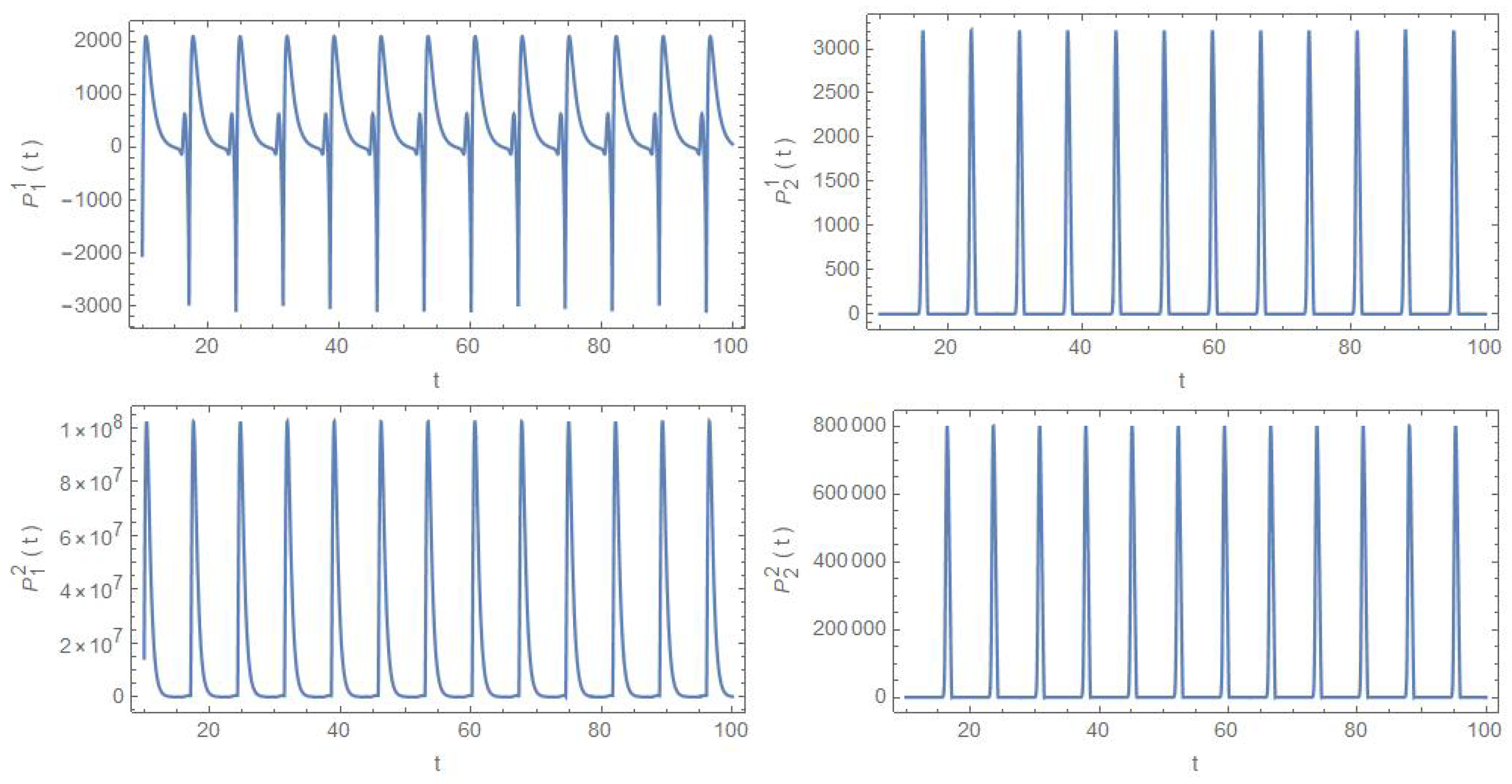
5. Chaotic Behavior of Oregonator Model

The trajectory behavior of deviation vector ${\xi }^i,i=1,2$ near fixed point is obtained by using the following Equation (8)

$$\begin{array}{c}\hfill \begin{array}{cc}\hfill & \frac{d^2{\xi }^1}{d{t}^2}+\frac{1}{ϵ}\left(2x^1+x^2-1\right)\frac{d{\xi }^1}{dt}+\frac{1}{ϵ}\left(x^1-q\right)\frac{d{\xi }^2}{dt}+\frac{1}{ϵ}\left(2y^1+y^2\right){\xi }^1+\frac{1}{ϵ}{y}^1{\xi }^2=0,\hfill \\ & \frac{d^2{\xi }^2}{d{t}^2}+\frac{1}{\delta }{x}^2\frac{d{\xi }^1}{dt}+\frac{1}{\delta }\left(q+\delta +x^1\right)\frac{d{\xi }^2}{dt}+\frac{1}{\delta }\left(x^2+y^2-f\right){\xi }^1+\frac{1}{\delta }{x}^1{\xi }^2=0.\hfill \end{array}\end{array}$$

(23)

The value of deviation vector can be obtained from its components ${\xi }^1$ and ${\xi }^2$ is given as

$$\xi =\sqrt{{\left[{\xi }^1\left(t\right)\right]}^2+{\left[{\xi }^2\left(t\right)\right]}^2.}$$

(24)

In order to obtain the chaotic behaviour of the Oregonator model, we introduce the Lyapunov exponents similar to the instability exponents. The Lyapunov exponents describes the rate of divergence of nearby trajectories, i.e., the presence of chaos in the system as

$${\Delta }_i\left(E\right)=\underset{t\to \infty }{lim}\frac{1}{t}ln\frac{{\xi }^i\left(t\right)}{{\dot{\xi }}^i\left(0\right)},i=1,2,$$

and

$$\Delta \left(E\right)=\underset{t\to \infty }{lim}\frac{1}{t}ln\frac{\xi \left(t\right)}{\dot{\xi }\left(0\right)},$$

Now, we examine the deviation vectors behaviour close to equilibrium positions. The initial conditions used to integrate the deviation equations are ${\xi }^1\left(t\right)={\xi }^2\left(t\right)=0,\dot{{\xi }^1}\left(t\right)={10}^{-10},\dot{{\xi }^2}\left(t\right)={10}^{-9}$ and values of the parameter are shown in their respective figures.

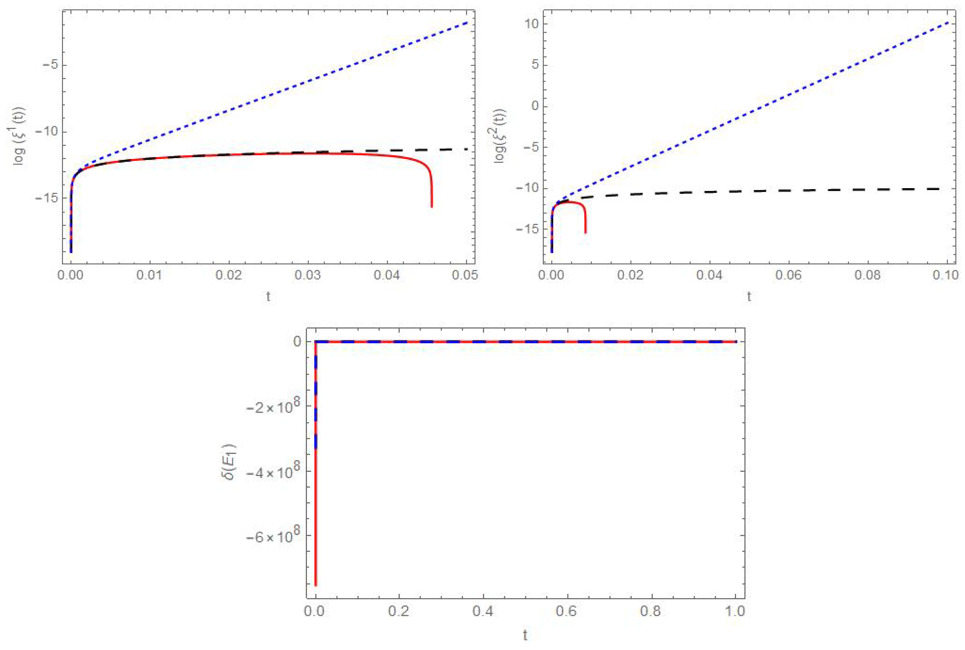
5.1. Behavior of the Deviation Vector near $E_0$

The dynamics of deviation vector near equilibrium point $E_0$ are calculated using Equation (23) as follows:

$$\begin{array}{cc}\hfill \frac{d^2{\xi }^1}{d{t}^2}-\frac{1}{ϵ}\frac{d{\xi }^1}{dt}-\frac{1}{ϵ}\frac{d{\xi }^2}{dt}& =0\hfill \\ \hfill \frac{d^2{\xi }^2}{d{t}^2}+\frac{(q+\delta )}{\delta }\frac{d{\xi }^2}{dt}-\frac{f}{\delta }{\xi }^1& =0\hfill \end{array}$$

(25)

The behaviour of components of the deviation curvature vector and instability exponents are shown in Figure 2.

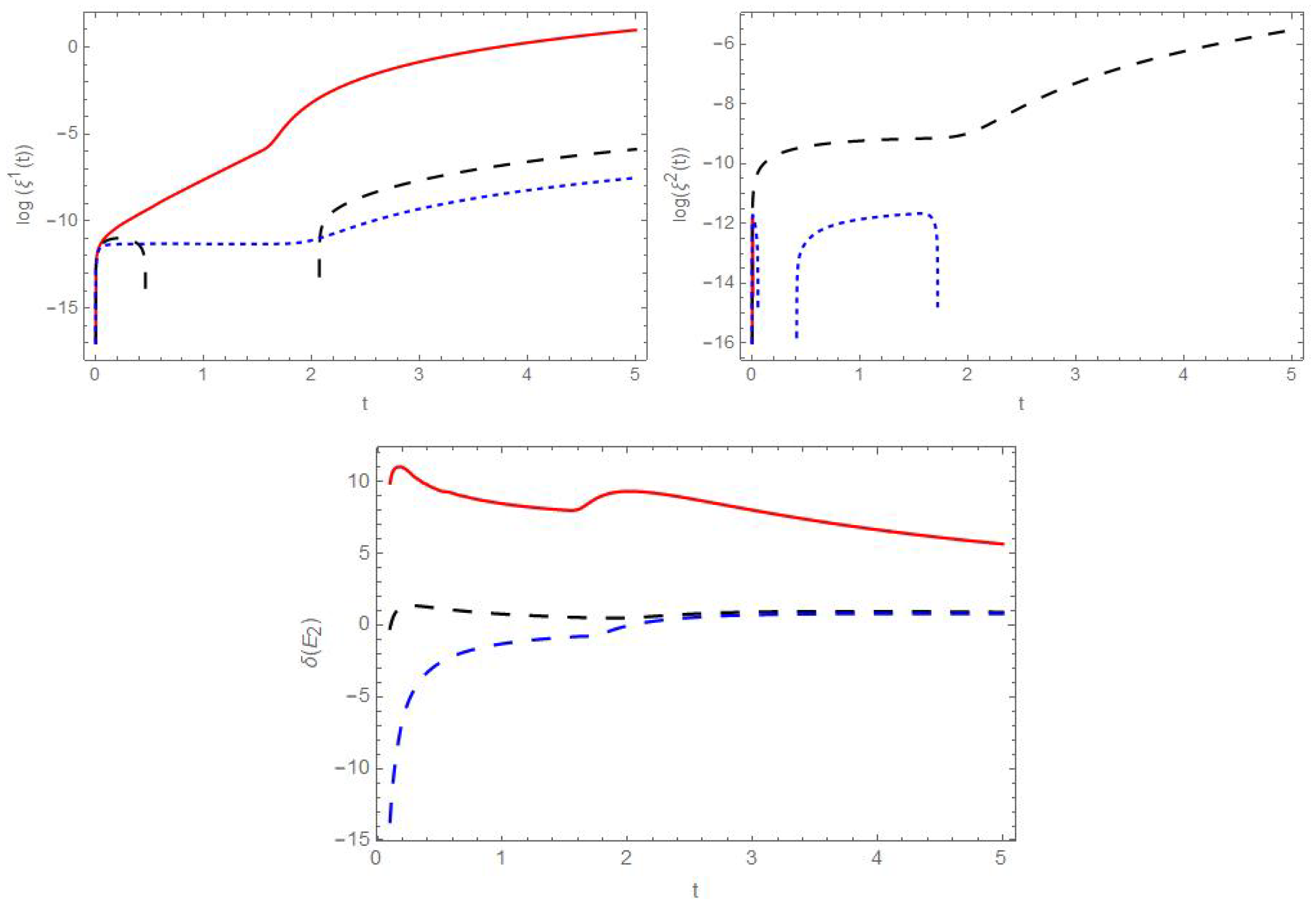
5.2. Behavior of the Deviation Vector near $E_1$

By using Equation (8), the dynamics of deviation vector near the equilibrium point $E_1$ are obtained as follows:

$$\begin{array}{cc}\hfill & \frac{d^2{\xi }^1}{d{t}^2}+\frac{1}{4ϵ}\left(4u-3v+w-4\right)\frac{d{\xi }^1}{dt}+\frac{1}{2ϵ}\left(u-v-2q\right)\frac{d{\xi }^2}{dt}=0\hfill \\ \hfill & \frac{d^2{\xi }^2}{d{t}^2}+\frac{1}{4\delta }(w+v)\frac{d{\xi }^1}{dt}+\frac{1}{2\delta }\left(2q+2\delta +u-v\right)\frac{d{\xi }^2}{dt}+\frac{1}{4\delta }\left(w+v-4f\right){\xi }^1+\frac{1}{2\delta }(u-v){\xi }^2=0\hfill \end{array}$$

The behaviour of components of the deviation curvature vector and instability exponents are shown in Figure 3.

5.3. Behavior of the Deviation Vector near $E_2$

The dynamics of deviation vector near equilibrium point $E_2$ are calculated using Equation (8) as follows:

$$\begin{array}{cc}\hfill & \frac{d^2{\xi }^1}{d{t}^2}+\frac{1}{4ϵ}(4u+3v+w-4)\frac{d{\xi }^1}{dt}+\frac{1}{2ϵ}(u+v-2q)\frac{d{\xi }^2}{dt}=0\hfill \\ \hfill & \frac{d^2{\xi }^2}{d{t}^2}+\frac{1}{4\delta }(w-v)\frac{d{\xi }^1}{dt}+\frac{1}{2\delta }\left(2q+2\delta +u+v\right)\frac{d{\xi }^2}{dt}+\frac{1}{4\delta }\left(w-v-4f\right){\xi }^1+\frac{1}{2\delta }(u+v){\xi }^2=0\hfill \end{array}$$

The behaviour of the components of the deviation curvature vector and instability exponents are shown in Figure 4.

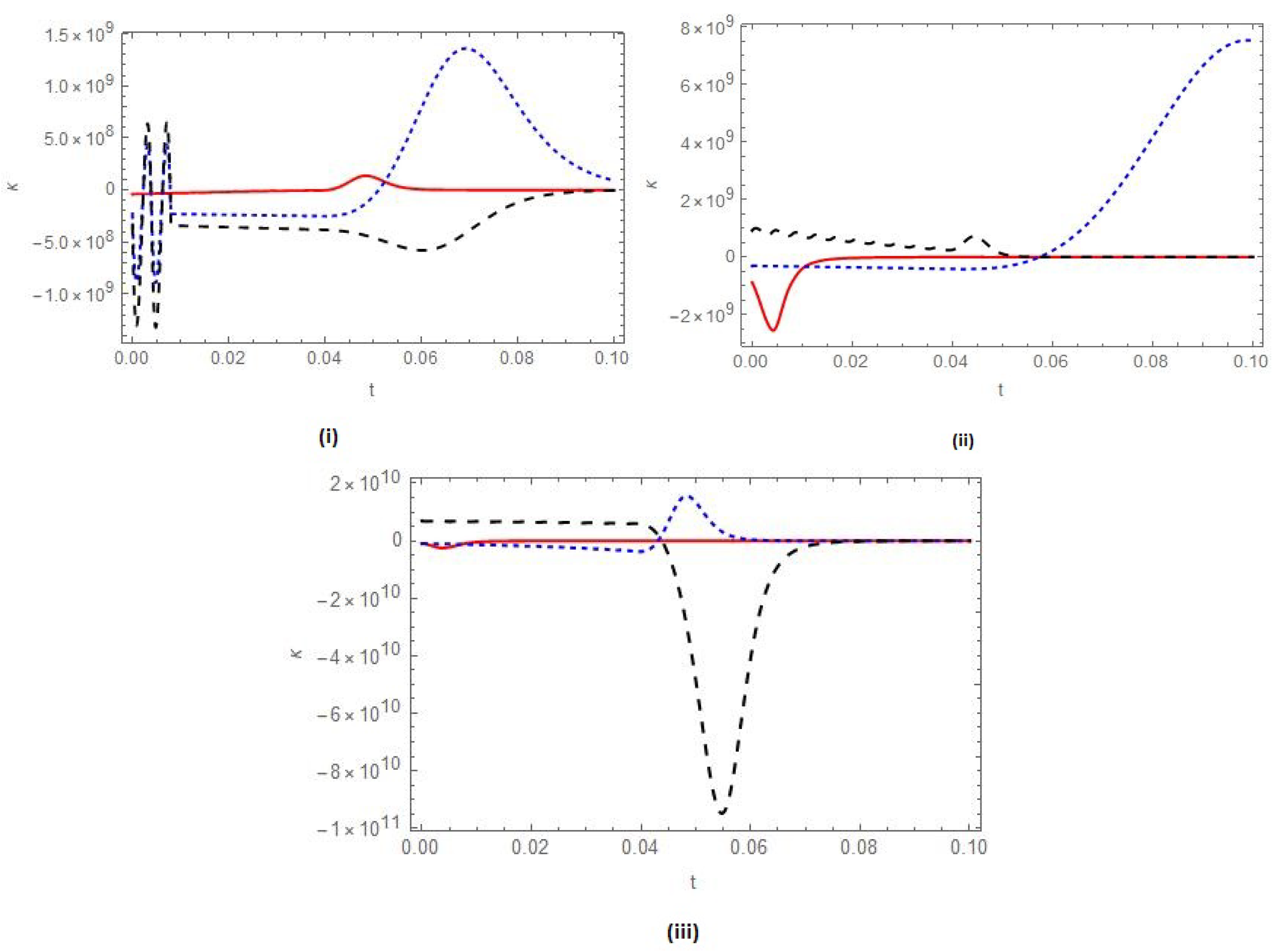
5.4. Curavture of the Deviation Tensor

The geometric curvature $\kappa$ of the curve $\xi \left(t\right)=({\xi }^1\left(t\right),{\xi }^2\left(t\right))$, examines the quantitative explanation of the deviation tensors behaviour which we define, according to the standard approach used in differential geometry of plane curve as [12]

$$\kappa =\frac{\dot{{\xi }^1}\left(t\right)\ddot{{\xi }^2}\left(t\right)-\dot{{\xi }^2}\left(t\right)\ddot{{\xi }^1}\left(t\right)}{{\{{\left[\dot{{\xi }^1}\left(t\right)\right]}^2+{\left[\dot{{\xi }^2}\left(t\right)\right]}^2\}}^{\frac{3}{2}}}$$

The chaotic behavior of the system is described by the curvature of the deviation vector. From Figure 5, we can see that for different value of parameters the curvature of the deviation vector is positive for very brief periods of time, hitting zero at specific times, moving into the region of negative values, and then, after temporarily tending toward zero, returning to positive values before moving back into the region of negative values.

The curvature of the deviation vector of the Oregonator model becomes zero at ${\xi }^1\left(t_0\right)={\xi }^2\left(t_0\right)$, and the time interval during which it changes sign is an symbol of the development of chaotic behavior.

The behaviour of the curvature deviation tensor are shown in Figure 5.

6. Jacobi Stability vs Linear Stability

In this section, we will consider the relationship between Jacobi stability and Linear stability at different equilibrium points. To compare both stability we first find Jacobian matrix for system (12) as follows:

$$J=\left(\begin{array}{c}\hfill \frac{1}{ϵ}(1-2x-y)\frac{1}{ϵ}(q-x)0\\ \hfill \frac{1}{\delta }(-y)\frac{1}{\delta }(-q-x)\frac{f}{\delta }\\ \hfill 10-1\end{array}\right)$$

Example 3.

If we take value of the parameters as $ϵ=2$, $\delta =0.004$, $q=0.08$, $f=1$ for the Jacobi matrix then the eigenvalues at equilibrium points $S\left(E_0\right)$, $S\left(E_1\right)$ and $S\left(E_2\right)$ are  $\{-19.9743,-1.2947,0,771729\}$, $\{63.2084,0.739929,-0.533817\}$ and $\{-84.3937,-0.552687,-0.0408065\},$ repectively.

At Equilibrium point $S\left(E_0\right)$ we have two negative and one positive eigenvalue, for the point $S\left(E_1\right)$ we obtain two positive and one negative eigenvalue and all eigenvalues are negative at the equilibrium point $S\left(E_2\right)$. Thus, both $S\left(E_0\right)$ and $S\left(E_1\right)$ points are linearly unstable while $S\left(E_2\right)$ is linearly stable. On comparing it with example 1, we found that equilibrium points  $E_0$ and $E_1$ of the system are both Jacobi and linearly unstable, while the point $E_2$, is Jacobi unstable but linearly stable.

Now, for the Jacobi matrix if we take a set of parameters $ϵ=0.10$, $\delta =0.004$, $q=0.0008$,

Example 4.

For $f=2.4$, the eigenvalues at equilibrium points $S\left(E_0\right)$, $S\left(E_1\right)$, $S\left(E_2\right)$ are  $\{10.0424,-0.62122\pm 0.539641i\}$, $\{323.185,40.5648,-0.375287\}$  and  $\{-7.44785,-0.557569\pm 0.57831i\}$ repectively.

For the first equilibrium point $S\left(E_0\right)$, we obtain one real eigenvalue and two complex conjugate and for $S\left(E_1\right)$ we get two positive and one negative real eigenvalue. At equilibrium point  $S\left(E_2\right)$, all three eigenvalues have negative real part. Thus, both $S\left(E_0\right)$ and $S\left(E_1\right)$ are linearly unstable while $S\left(E_2\right)$ is linearly stable. Therefore, on comparing it with example 2, we found that equilibrium points $E_0$ and $E_1$ of the system are both Jacobi and linearly unstable, while the point $E_2$, is Jacobi unstable but linearly stable.

Example 5.

For $f=1$, the eigenvalues at equilibrium points $S\left(E_0\right)$, $S\left(E_1\right)$, $S\left(E_2\right)$ are  $\{10.0178,-0.608883\pm 0.168974i\}$,$\{3.231\pm 7.76734i,-0.0573755\}$  and  $\{-12.9551,4.291,0.0710088\}$ respectively. Equilibrium point $S\left(E_0\right)$ has one positive eigenvalue and a conjugate pair of eigenvalues with negative real part. Equilibrium points $S\left(E_1\right)$ and $S\left(E_2\right)$ has one negative and two positive eigenvalues. Thus, both  $S\left(E_1\right)$ and $S\left(E_2\right)$ are linearly unstable, while $S\left(E_1\right)$ is linearly stable.

Examples 4 and 5, show the value of stoichiometric factor as we can see that the system changes its stability at equilibrium point $S\left(E_2\right)$, with the small change in the value of f. Hence, the parameter f is deeply linked to the ocillation rise in the chemical reaction.

7. Conclusions

In the paper, we have looked at the stability analysis of the Oregonator model for BZ-reaction from the perspective of the KCC theory, according to which the geometric properties of the geodesic equations for Finsler space, which are the equivalent of the given system and can be used to deduce the dynamical stability properties of dynamical systems. We first transformed the first order differential equation of the Oregonator model into a system of second order differential equations. We have introduced the instability exponent and the curvature of the deviation vector for the Oregonator model in order to describe the behavior of the trajectories around the equilibrium points. We have also shown the graphical representations of deviation vector components ${\xi }^1\left(t\right)$ and ${\xi }^2\left(t\right)$ in a logrithmic scale and instability exponents near all three equilibrium points for different set of parameters in Figure 2, Figure 3 and Figure 4. Through the curve $\xi \left(t\right)$ transition moment from positive to negative values, it can be directly related to the chaotic behavior of the trajectories. We expressed the geometric quantities of KCC theory in terms of the Jacobian matrix of the linearized system in order to understand the relationship between the Jacobi stability and the linear stability.

This study presents the conditions for Jacobi stability at the equilibrium points of the Oregonator model. It demonstrates that, at the origin the system is always Jacobi unstable, whereas the Jacobi stability of the remaining two equilibrium points is dependent on the particular set of parameter values present in the system. In Mathematical modelling of the BZ reaction the stoichiometric factor has been used as a bifurcation parameter. The phenomenon denotes the transition between the stationary and oscillation during the chemical reaction. The present analysis provides the role of stoichiometric factor as a small increase or decrease in the value leads us to a different stability state of the system. In brief, our analysis of the Belousov–Zhabotinsky (BZ) reaction, a well-established example of an oscillating chemical reaction, using the KCC theory reveals that the system possesses a dual nature (stability and instability) of the system. The analysis emphasizes the coexistence of Jacobi stability and instability. Furthermore, the system exhibits characteristics of both linear stability and instability. This investigation enhances our understanding of the complex dynamics intrinsic in oscillating chemical reactions, thereby making a significant contribution to the wider comprehension of dynamic systems.

References

1. Winfree, A.T. The prehistory of the Belousov-Zhabotinsky oscillator. J. Chem. Educ. 1984, 61, 661. [Google Scholar] [CrossRef]
2. Field, R.J.; Noyes, R.M. Oscillations in chemical systems. IV. Limit cycle behavior in a model of a real chemical reaction. J. Chem. Phys. 1974, 60, 1877–1884. [Google Scholar] [CrossRef]
3. Lotka, A.J. Undamped oscillations derived from the law of mass action. J. Am. Chem. Soc. 1920, 42, 1595–1599. [Google Scholar] [CrossRef]
4. Nicolis, G. Stability and dissipative structures in open systems far from equilibrium. Adv. Chem. Phys. 1971, 19, 209–324. [Google Scholar]
5. Cassani, A.; Monteverde, A.; Piumetti, M. Belousov-Zhabotinsky type reaction: The non-linear behavior of chemical systems. J. Math. Chem. 2021, 59, 792–826. [Google Scholar] [CrossRef]
6. Pullela, S.R.; Cristancho, D.; He, P.; Luo, D.; Hall, K.R.; Cheng, Z. Temperature dependence of the Oregonator model for the Belousov-Zhabotinsky reaction. Phys. Chem. Chem. Phys. 2009, 11, 4236–4243. [Google Scholar] [CrossRef]
7. Kosambi, D.D. Parallelism and path-space. Math. Z. 1933, 37, 608–818. [Google Scholar] [CrossRef]
8. Cartan, E. Observations sur le memoire precedent. Math. Z. 1933, 37, 619–622. [Google Scholar] [CrossRef]
9. Chern, S.S. Sur la geometrie d’um systemme d’equation differentielles du second ordre. Bull. Sci. Math. 1939, 63, 206–212. [Google Scholar]
10. Antonelli, P.L.; Ingarden, R.S.; Matsumoto, M. The Theories of Sprays and Finsler Spaces with Application in Physics and Biology; Kluwer Academic Publishers: Dordrecht, The Netherlands, 1993. [Google Scholar]
11. Antonelli, P.L. Equivalence Problem for Systems of Second Order Ordinary Differential Equations. In Encyclopedia of Mathematics; Kluwer Academic Publishers: Dordrecht, The Netherlands, 2000. [Google Scholar]
12. Harko, T.; Ho, C.Y.; Leung, C.S.; Yip, S. Jacobi stability analysis of Lorenz system. Int. J. Geom. Methods Mod. Phys. 2015, 12, 1550081. [Google Scholar] [CrossRef]
13. Gupta, M.K.; Yadav, C.K. Jacobi stability analysis of modified Chua circuit system. Int. J. Geom. Methods Mod. Phys. 2017, 14, 121–142. [Google Scholar] [CrossRef]
14. Gupta, M.K.; Yadav, C.K. Jacobi stability analysis of Rikitake system. Int. J. Geom. Methods Mod. Phys. 2016, 13, 1650098. [Google Scholar] [CrossRef]
15. Gupta, M.K.; Yadav, C.K. KCC theory and its application in a tumor growth model. Math. Methods Appl. Sci. 2017, 40, 7470–7487. [Google Scholar] [CrossRef]
16. Gupta, M.K.; Yadav, C.K. Rabinovich-Fabrikant system in view point of KCC theory in Finsler geometry. J. Interdiscip. Math. 2019, 22, 219–241. [Google Scholar] [CrossRef]
17. Gupta, M.K.; Yadav, C.K.; Gupta, A.K. A geometrical study of Wang-Chen system in view of KCC theory. TWMS J. Appl. Eng. Math. 2020, 10, 1064. [Google Scholar]
18. Kumar, M.; Mishra, T.N.; Tiwari, B. Stability analysis of Navier–Stokes system. Int. J. Geom. Methods Mod. Phys. 2019, 16, 1950157. [Google Scholar] [CrossRef]
19. Munteanu, F. On the Jacobi Stability of Two SIR Epidemic Patterns with Demography. Symmetry 2023, 15, 1110. [Google Scholar] [CrossRef]
20. Munteanu, F.; Grin, A.; Musafirov, E.; Pranevich, A.; Şterbeţi, C. About the Jacobi Stability of a Generalized Hopf–Langford System through the Kosambi–Cartan–Chern Geometric Theory. Symmetry 2023, 15, 598. [Google Scholar] [CrossRef]
21. Yadav, C.K.; Gupta, M.K. Jacobi stability Analysis of Lu system. J. Int. Acad. Phys. Sci. 2019, 23, 123–142. [Google Scholar]
22. Liu, Y.; Huang, Q.; Wei, Z. Dynamics at infinity and Jacobi stability of trajectories for the Yang-Chen system. Discrete Contin. Dyn. Syst. Ser. 2021, 26, 3357–3380. [Google Scholar] [CrossRef]
23. Yamasaki, K.; Yajima, T. KCC analysis of a one-dimensional system during catastrophic shift of the Hill function: Douglas tensor in the nonequilibrium region. Int. J. Bifurc. Chaos 2020, 30, 2030032. [Google Scholar] [CrossRef]
24. Feng, C.; Qiujian, H.; Liu, Y. Jacobi analysis for an unusual 3D autonomous system. Int. J. Geom. Methods Mod. Phys. 2020, 17, 2050062. [Google Scholar] [CrossRef]
25. Liu, Y.; Chen, H.; Lu, X.; Feng, C.; Liu, A. Homoclinic orbits and Jacobi stability on the orbits of Maxwell–Bloch system. Appl. Anal. 2022, 101, 4377–4396. [Google Scholar] [CrossRef]
26. Chen, B.; Liu, Y.; Wei, Z.; Feng, C. New insights into a chaotic system with only a Lyapunov stable equilibrium. Math. Methods Appl. Sci. 2020, 43, 9262–9279. [Google Scholar] [CrossRef]
27. Yamasaki, K.; Yajima, T. Kosambi–Cartan–Chern Stability in the Intermediate Nonequilibrium Region of the Brusselator Model. Int. J. Bifurc. Chaos 2022, 32, 2250016. [Google Scholar] [CrossRef]
28. Yamasaki, K.; Yajima, T. Kosambi–Cartan–Chern Analysis of the Nonequilibrium Singular Point in One-Dimensional Elementary Catastrophe. Int. J. Bifurc. Chaos 2022, 32, 2250053. [Google Scholar] [CrossRef]
29. Boehmer, C.G.; Harko, T.; Sabau, S.V. Jacobi stability analysis of dynamical systems-applications in gravitation and cosmology. Adv. Theor. Math. Phys. 2012, 16, 1145–1196. [Google Scholar] [CrossRef]
30. Gupta, M.K.; Yadav, C.K. Jacobi stability analysis of Rossler system. Int. J. Bifurc. Chaos 2017, 27, 1750056. [Google Scholar] [CrossRef]
31. Rahman, Q.I.; Schmeisser, G. Analytic Theory of Polynomials; London Mathematical Society Monographs, New Series; Oxford University Press: Oxford, UK, 2002; Volume 26. [Google Scholar]
Figure 1. Time variation of components of deviation tensor P 1 1 (left top figure), P 2 1 (right top figure), P 1 2 (left bottom figure) and P 2 1 (right bottom figure) for parameters values ϵ = 0.10 , δ = 0.0004 , q = 0.0008 and f = 1 . The initial conditions for the numerical integration system are x 1 ( 0 ) = x 2 ( 0 ) = x 3 ( 0 ) = 5 .
Axioms 12 01133 g001
Figure 2. Time variation of the deviation vector components ξ 1 ( t ) (left figure) and ξ 2 ( t ) (right figure), in a logarithmic scale and instability exponents δ ( E 0 ) , near the equilibrium point E 0 , for ϵ = 0.10 , δ = 0.0004 , q = 0.0008 , f = 1 (Solid Red), for ϵ = 1 , δ = 4 , q = 0.0008 , f = 0.5 (Black), for ϵ = 0.10 , δ = 0.004 , q = 0.8 , f = 2.4 (Blue). The initial conditions used to integrate the deviation equations are ξ 1 ( t ) = ξ 2 ( t ) = 0 , ξ ˙ 1 ( t ) = 10 10 , ξ ˙ 2 ( t ) = 10 9 .
Axioms 12 01133 g002
Figure 3. Time variation of the deviation vector components in a logarithmic scale ξ 1 ( t ) (left figure) and ξ 2 ( t ) (right figure), δ ( E 1 ) , near the equilibrium point E 1 , for ϵ = 0.10 , δ = 0.0004 , q = 0.0008 , f = 1 (Solid Red), for ϵ = 1 , δ = 0.4 , q = 0.0008 , f = 0.5 (Black), for ϵ = 0.10 , δ = 0.004 , q = 0.8 , f = 2.4 (Blue). The initial conditions used to integrate the deviation equations are ξ 1 ( t ) = ξ 2 ( t ) = 0 , ξ ˙ 1 ( t ) = 10 10 , ξ ˙ 2 ( t ) = 10 9 .
Axioms 12 01133 g003
Figure 4. Time variation of the deviation vector components in a logarithmic scale ξ 1 ( t ) (left figure) and ξ 2 ( t ) (right figure), δ ( E 2 ) , near the equilibrium point E 2 , for ϵ = 0.10 , δ = 0.0004 , q = 0.0008 , f = 1 (Solid Red), for ϵ = 1 , δ = 4 , q = 0.0008 , f = 0.5 (Black), for ϵ = 0.10 , δ = 0.004 , q = 0.8 , f = 2.4 (Blue). The initial conditions used to integrate the deviation equations are ξ 1 ( t ) = ξ 2 ( t ) = 0 , ξ ˙ 1 ( t ) = 10 10 , ξ ˙ 2 ( t ) = 10 9 .
Axioms 12 01133 g004
Figure 5. Time variation of curvature κ for E 0 (above left), E 1 (above right), E 2 (below) for parameter values ϵ = 0.10 , δ = 0.0004 , q = 0.0008 , f = 1 (Red), for ϵ = 1 , δ = 0.04 , q = 0.008 , f = 0.5 (Blue), (i) for ϵ = 0.50 , δ = 0.04 , q = 0.008 , f = 0.8 (Black), (ii) for ϵ = 0.30 , δ = 0.004 , q = 0.08 , f = 0.7 (Black), (iii) for ϵ = 0.05 , δ = 0.4 , q = 0.008 , f = 0.7 (Black). The initial conditions used to integrate the deviation equations are ξ 1 ( t ) = ξ 2 ( t ) = 0 , ξ ˙ 1 ( t ) = 10 10 , ξ ˙ 2 ( t ) = 10 9 .
Axioms 12 01133 g005