On the Crossing Bridge between Two Kirchhoff–Love Plates

Abstract

The paper is concerned with equilibrium problems for two elastic plates connected by a crossing elastic bridge. It is assumed that an inequality-type condition is imposed, providing a mutual non-penetration between the plates and the bridge. The existence of solutions is proved, and passages to limits are justified as the rigidity parameter of the bridge tends to infinity and to zero. Limit models are analyzed. The inverse problem is investigated when both the displacement field and the elasticity tensor of the plate are unknown. In this case, additional information concerning a displacement of a given point of the plate is assumed be given. A solution existence of the inverse problem is proved.

1. Introduction

Bridged structures are very popular for solving connecting problems. Such structures may be different in type, and their quality depends on the purposes addressed. In this paper, we analyze the structure consisting of two Kirchhoff–Love elastic plates and a junction (bridge) that is in contact with the plates. To describe the behavior of the bridge, we use the Euler–Bernoulli beam model. The junction has the displacement coinciding with the displacement of the plates at two fixed points. Moreover, an inequality-type restriction is assumed to be imposed for the solution to provide a mutual non-penetration between the plates and the bridge. This approach implies that the problem is formulated as a free boundary one.

During the last years, boundary-value problems in elasticity with inequality-type boundary conditions have been under active study. We can refer the reader to the books [1,2] containing results for crack models with the non-penetration boundary conditions for a wide class of elasticity problems. There are many papers related to thin inclusions incorporated into elastic bodies. In the case of delamination of the surrounding elastic body from the inclusion, one more difficulty appears since we obtain an interfacial crack. We pay attention to the paper [3] where an equilibrium problem for two elastic plates is analyzed in the case of thin incorporated inclusion and Neumann type boundary conditions for the plate. Different properties of solutions in equilibrium problems for elastic bodies with thin rigid, semi-rigid, and elastic inclusions and cracks are analyzed in [4,5,6,7,8,9,10,11,12,13] and many other papers. In [14,15,16], one can find models for the analysis of non-homogeneous elastic bodies. Note that a derivation of models for elastic bodies with thin inclusions usually takes into account changing physical and geometrical parameters [17,18,19]. Contact problems for elastic plates with thin elastic structures were analyzed in [20,21]. We can also mention a number of applied studies related to thin inclusions of different nature in elastic bodies [22,23,24,25,26,27,28,29]. An application of the finite element method for planar mechanical elastic systems can be found in [30]. As for inverse problems in elasticity, the literature in this field is very vast. We will only mention the articles [31,32] and the links in them.

The structure of the paper is as follows. Section 2 addresses variational and differential formulations of the equilibrium problem. Passages to limits, as a rigidity parameter of the bridge tends to infinity and to zero, are investigated in Section 3 and Section 4. We provide a justification of the limit procedure and analyze the limit models. Section 5 is concerned with the analysis of the inverse problem.

2. Setting the Problem

Let ${\Omega }_1,{\Omega }_2\subset {\mathbb{R}}^2$ be bounded domains with Lipschitz boundaries ${\Gamma }^1,{\Gamma }^2,$ respectively, such that ${\overline{\Omega }}_1\cap {\overline{\Omega }}_2=\varnothing .$ Assume that ${\Gamma }^i$ is divided into two smooth parts ${\Gamma }_N^i$ and ${\Gamma }_D^i,\mathrm{meas}{\Gamma }_D^i>0,i=1,2.$ We set $b=(-2,2)\times \left\{0\right\},b_1=(-2,-1)\times \left\{0\right\},b_2=(1,2)\times \left\{0\right\},b_0=(-1,1)\times \left\{0\right\}.$ Moreover, we assume that $b_i\subset {\Omega }_i,$ and b crosses ${\Gamma }_N^i,$$b_0\cap {\Omega }_i=\varnothing ,i=1,2,$ see Figure 1. Denote by $\nu =(0,1),n=(n_1,n_2)$ unit normal vectors to $b,{\Gamma }^i$, respectively, and set $\Omega ={\Omega }_1\cup {\Omega }_2,$ ${\Omega }_b=\Omega \backslash \overline{b}.$

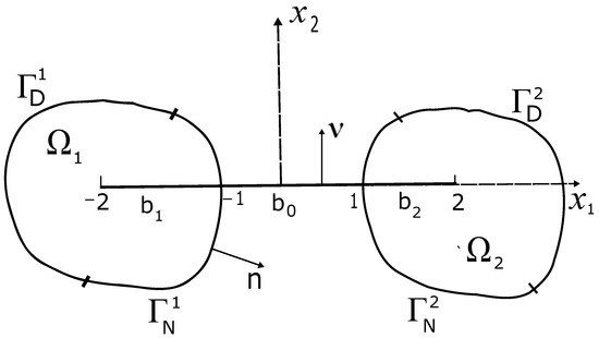
Figure 1. Elastic plates ${\Omega }_1,{\Omega }_2$ with crossing bridge b.

The set $\Omega$ corresponds to two elastic plates, and b fits to a thin elastic crossing bridge between two plates. We describe b in the frame of the Euler–Bernoulli beam model. In what follows, the crossing bridge b will be characterized by a rigidity parameter $\alpha >0.$ At the first step, this parameter is fixed being equal to 1, and in the sequel we analyze passages to the limit as $\alpha$ goes to infinity and to zero.

Let w be a scalar-valued function. We use the notations $w_n=\frac{\partial w}{\partial n},w_{\nu }=\frac{\partial w}{\partial \nu }.$ If $M=\left\{M_{ij}\right\},i,j=1,2,$ then $\nabla \nabla M=M_{ij,ij}.$ We also put $\nabla \nabla w=\left\{w_{,ij}\right\},i,j=1,2.$ Summation convention over repeated indices is used; all functions with two lower indices are assumed to be symmetric in those indices.

In the domains ${\Omega }_1,{\Omega }_2$, elasticity tensors $A=\left\{a_{ijkl}\right\},B=\left\{b_{ijkl}\right\},i,j,k,l=1,2,$ are considered with the usual properties of symmetry and positive definiteness,

$$\begin{array}{c}\hfill a_{ijkl}\in L^{\infty }\left({\Omega }_1\right),\\ \hfill A\xi ·\xi \ge c_0{\left|\xi \right|}^2\forall \xi =\left\{{\xi }_{ij}\right\},{\xi }_{ji}={\xi }_{ij},c_0=const>0.\end{array}$$

(1)

Similar properties are fulfilled for the tensor B on ${\Omega }_2.$

We introduce notations for a bending moment $M_n$ and a transverse force $T^n=T^n\left(M\right)$ on the boundaries of the plates,

$$M_n=-M_{ij}{n}_j{n}_i;T^n=-M_{ij,j}{n}_i-M_{ij,k}{\tau }_k{\tau }_j{n}_i,({\tau }_1,{\tau }_2)=(-n_2,n_1).$$

(2)

In this case, for smooth functions $w,M=\left\{M_{ij}\right\},i,j=1,2,$ the following Green’s formula holds, see [2], Section 1.2.3,

$$-\underset{{\Omega }_i}{\int }M·\nabla \nabla w=-\underset{{\Omega }_i}{\int }w\nabla \nabla M+\underset{{\Gamma }^i}{\int }{M}_n{w}_n-\underset{{\Gamma }^i}{\int }{T}^{n}w,i=1,2.$$

Since the domain ${\Omega }_b$ with the cut $b_1\cup b_2$ is a union of the domains ${\Omega }_1\backslash b_1$ and ${\Omega }_2\backslash b_2$, the above Green’s formula allows us to write Green’s formula for ${\Omega }_b,$

$$\begin{array}{c}\hfill -\underset{{\Omega }_b}{\int }M·\nabla \nabla w=-\underset{{\Omega }_b}{\int }w\nabla \nabla M-\underset{b_1\cup b_2}{\int }\left[M_{\nu }\right]w_{\nu }+\underset{b_1\cup b_2}{\int }\left[T^{\nu }\right]w\\ \hfill +\underset{{\Gamma }^1\cup {\Gamma }^2}{\int }{M}_n{w}_n-\underset{{\Gamma }^1\cup {\Gamma }^2}{\int }{T}^{n}w,\end{array}$$

(3)

where $\left[h\right]=h^{+}-h^{-}$ is a jump of a function h on $b_i;$$h^{\pm }$ are the traces of h on the crack faces $b_i^{\pm },i=1,2$. The signs ± fit to positive and negative directions of $\nu ;$ the values $M_{\nu },T^{\nu }$ with the normal vector $\nu$ are defined on b similar to (2).

In view of the above notations, an equilibrium problem for the plates ${\Omega }_1,{\Omega }_2$ and the crossing bridge b is formulated as follows. Given external forces $f\in L^2(\Omega ),g\in L^2\left(b\right)$ acting on the plates and the crossing bridge, respectively, we have to find a displacement of the plates $w$; a moment tensor $M=\left\{M_{ij}\right\},i,j=1,2,$ defined in $\Omega ,{\Omega }_b,$ respectively; and a crossing bridge displacement v defined on b such that

$$\begin{array}{c}\hfill \nabla \nabla M+f=0\mathrm{in}{\Omega }_b,\end{array}$$

(4)

$$\begin{array}{c}\hfill M+E\nabla \nabla w=0\mathrm{in}{\Omega }_b,\end{array}$$

(5)

$$\begin{array}{c}\hfill v_{,1111}=g\mathrm{on}{b}_0;v_{,1111}=-\left[T^{\nu }\right]+g\mathrm{on}{b}_1\cup b_2,\end{array}$$

(6)

$$\begin{array}{c}\hfill w=w_n=0\mathrm{on}{\Gamma }_D^1\cup {\Gamma }_D^2;M_n=T^n=0\mathrm{on}{\Gamma }_N^1\cup {\Gamma }_N^2,\end{array}$$

(7)

$$\begin{array}{c}\hfill w(\pm 2,0)=0;v=v_{,11}=0\mathrm{as}{x}_1=-2,2,\end{array}$$

(8)

$$\begin{array}{c}\hfill v-w\ge 0,\left[T^{\nu }\right]\le 0,(v-w)\left[T^{\nu }\right]=0\mathrm{on}{b}_1\cup b_2,\end{array}$$

(9)

$$\begin{array}{c}\hfill \left[w\right]=\left[w_{\nu }\right]=0,\left[M_{\nu }\right]=0\mathrm{on}{b}_1\cup b_2,\end{array}$$

(10)

$$\begin{array}{c}\hfill \left[v(\pm 1)\right]=\left[v_{,1}(\pm 1)\right]=0,\left[v_{,11}(\pm 1)\right]=\left[v_{,111}(\pm 1)\right]=0.\end{array}$$

(11)

Here, $\left[h\right(a\left)\right]=h(a+0)-h(a-0);$$w_{,1}=\frac{\partial w}{\partial x_1},(x_1,x_2)\in \Omega .$ The tensor E is equal to $A,B$ in ${\Omega }_1,{\Omega }_2,$ respectively. Functions defined on b we identify with functions of the variable $x_1.$

Relations (4) and (5) are the equilibrium equations for the Kirchhoff–Love elastic plates ${\Omega }_1,{\Omega }_2$ and the constitutive law; (6) is the Euler–Bernoulli equilibrium equations for the crossing bridge parts $b_i$, see [1,2]. The right-hand side $-\left[T^{\nu }\right]$ in (6) describes forces acting on $b_1\cup b_2$ from the elastic plates. The first inequality in (9) provides a non-penetration between the plates and the bridge. Relation (11) provides glue conditions at the points where the bridge b crosses the external boundaries of the elastic plates. Note that, by (9), the contact set between the plates and the bridge is unknown.

We can provide a variational formulation of the problem (4)–(11). Introduce the space

$$W=H^{2,0}\left(b\right)\times H_D^{2,0}(\Omega )$$

with the norm

$${\parallel (v,w)\parallel }_W^2={\parallel v\parallel }_{H^{2,0}\left(b\right)}^2+{\parallel w\parallel }_{H_D^{2,0}(\Omega )}^2,$$

where $H^{2,0}\left(b\right),H_D^{2,0}(\Omega )$ are the usual Sobolev spaces,

$$\begin{array}{c}\hfill H_D^{2,0}(\Omega )=\{w\in H^2(\Omega )|w=w_n=0\mathrm{on}{\Gamma }_D^1\cup {\Gamma }_D^2;w(\pm 2,0)=0\},\\ \hfill H^{2,0}\left(b\right)=\{v\in H^2\left(b\right)|v(\pm 2)=0\},\end{array}$$

and consider the energy functional $\Pi :W\to \mathbb{R},$

$$\Pi (v,w)=\frac{1}{2}C(w,w)-\underset{\Omega }{\int }fw+\frac{1}{2}\underset{b}{\int }{v}_{,11}^2-\underset{b}{\int }gv.$$

Here,

$$C(w,\overline{w})=\underset{{\Omega }_1}{\int }{a}_{ijkl}{w}_{,kl}{\overline{w}}_{,ij}+\underset{{\Omega }_2}{\int }{b}_{ijkl}{w}_{,kl}{\overline{w}}_{,ij}.$$

Denote by S the set of admissible displacements,

$$S=\{(v,w)\in W|v-w\ge 0\mathrm{on}{b}_1\cup b_2\}$$

and consider the problem:

$$\mathrm{Find}(v,w)\in S\mathrm{such}\mathrm{that}\Pi (v,w)=\underset{S}{inf}\Pi .$$

This minimization problem has a unique solution since the functional $\Pi$ is weakly lower semicontinuous and coercive. The coercivity of the functional $\Pi$ follows from the Dirichlet boundary conditions on the sets ${\Gamma }_D^i$ for the function w and conditions $v(\pm 2)=0$. The set S is weakly closed. The solution of the problem satisfies the following variational inequality

$$(v,w)\in S,$$

(12)

$$\begin{array}{c}\hfill C(w,\overline{w}-w)-\underset{\Omega }{\int }f(\overline{w}-w)\\ \hfill +\underset{b}{\int }{v}_{,11}({\overline{v}}_{,11}-v_{,11})-\underset{b}{\int }g(\overline{v}-v)\ge 0\forall (\overline{v},\overline{w})\in S.\end{array}$$

(13)

Theorem 1. 

Problem formulations (4)–(13) are equivalent for smooth solutions.

Proof. 

Assume that (12) and (13) hold. We can substitute in (13) test functions of the form $(\overline{v},\overline{w})=(v,w)\pm (0,\phi ),\phi \in C_0^{\infty }\left({\Omega }_b\right).$ This provides the equilibrium Equation (4) fulfilled in the distributional sense. Next, test functions of the form $(\overline{v},\overline{w})=(v,w+\phi )$ can be substituted in (13), where $\phi \in C_0^{\infty }(\Omega ),$$\phi \le 0$ on $b_1\cup b_2;\phi (\pm 2,0)=0.$ Taking into account the equilibrium Equation (4) and Green Formula (3), we obtain

$$-\underset{b_1\cup b_2}{\int }\left[M_{\nu }\right]{\phi }_{\nu }+\underset{b_1\cup b_2}{\int }\left[T^{\nu }\right]\phi \ge 0.$$

From here, it follows

$$\left[M_{\nu }\right]=0,\left[T^{\nu }\right]\le 0\mathrm{on}{b}_1\cup b_2.$$

(14)

Now, test functions of the form $(\overline{v},\overline{w})=(v+\psi ,w+\phi )$ are substituted in (13), $(\psi ,\phi )\in S,\mathrm{supp}\psi \subset (b_1\cup b_2).$ This gives

$$C(w,\phi )-\underset{\Omega }{\int }f\phi +\underset{b}{\int }{v}_{,11}{\psi }_{,11}-\underset{b}{\int }g\psi \ge 0.$$

Consequently, by using the Green Formula (3), in view of (4), (14), we derive

$$\underset{b_1\cup b_2}{\int }\left[T^{\nu }\right]\phi +\underset{b}{\int }{v}_{,1111}\psi -\underset{b}{\int }g\psi \ge 0.$$

Choosing the above inequality $\psi =\phi$ on $b_1\cup b_2$, the following equation

$$v_{,1111}=-\left[T^{\nu }\right]+g\mathrm{on}{b}_1\cup b_2$$

(15)

is derived. To proceed, take test functions of the form $(\overline{v},\overline{w})=(v\pm \psi ,w)$ in (3), $\mathrm{supp}\psi \subset b_0.$ The following relation is obtained:

$$\underset{b_0}{\int }{v}_{,11}{\psi }_{,11}-\underset{b_0}{\int }g\psi =0.$$

Thus,

$$v_{,1111}=g\mathrm{on}{b}_0.$$

(16)

Now, we are aiming to derive the last relation of (9). Assume that the inequality $v\left(x_0\right)-w\left(x_0\right)>0$ holds at a point $x_0\in b_1\cup b_2.$ In this case, we can take $(\overline{v},\overline{w})=(v,w)\pm \epsilon (\psi ,\phi )$ as a test function in (13), where the support of $\psi$ belongs to a small neighborhood of $x_0;$ the support of $\phi$ belongs to a small neighborhood of the point $(x_0,0)$, and $\epsilon$ is small. This implies

$$C(w,\phi )-\underset{\Omega }{\int }f\phi +\underset{b}{\int }{v}_{,11}{\psi }_{,11}-\underset{b}{\int }g\psi =0.$$

By (3), (4), and (14), we obtain the relation

$$\underset{b_1\cup b_2}{\int }\left[T^{\nu }\right]\phi +\underset{b}{\int }{v}_{,1111}\psi -\underset{b}{\int }g\psi =0.$$

In particular, this provides

$$\begin{array}{c}\hfill \left[T^{\nu }\right]=0\mathrm{in} \mathrm{a} \mathrm{neighborhood} \mathrm{of} \mathrm{the} \mathrm{point}{x}_0.\end{array}$$

This means that

$$(v-w)\left[T^{\nu }\right]=0\mathrm{on}{b}_1\cup b_2.$$

The next step of our reasoning is to derive boundary conditions for v at the points $\pm 1,\pm 2$ and the last condition of (7). To this end, we take test function in (13) of the form $(\overline{v},\overline{w})=(v,w)\pm (\psi ,\phi ),(\psi ,\phi )\in W,$$\phi =\psi$ on $b_1\cup b_2.$ It provides the equality

$$C(w,\phi )-\underset{\Omega }{\int }f\phi +\underset{b_0}{\int }{v}_{,11}{\psi }_{,11}+\underset{b_1\cup b_2}{\int }{v}_{,11}{\psi }_{,11}-\underset{b}{\int }g\psi =0.$$

Applying the Green Formula (3), this relation implies

$$\begin{array}{c}\hfill -\underset{{\Omega }_b}{\int }\nabla \nabla M·\phi -\underset{{\Omega }_b}{\int }f\phi +\underset{b_0}{\int }{v}_{,1111}\psi +\underset{b_1\cup b_2}{\int }{v}_{,1111}\psi \\ \hfill -\underset{b_1\cup b_2}{\int }\left[M_{\nu }\right]{\phi }_{\nu }+\underset{b_1\cup b_2}{\int }\left[T^{\nu }\right]\phi +\underset{{\Gamma }^1\cup {\Gamma }^2}{\int }{M}_n{\phi }_n-\underset{{\Gamma }^1\cup {\Gamma }^2}{\int }{T}^n\phi \\ \hfill -\underset{b_0}{\int }g\psi -\underset{b_1\cup b_2}{\int }g\psi -v_{,111}\psi {{|}_{x_1=-1}^{x_1=1}+v_{,11}{\psi }_{,1}|}_{x_1=-1}^{x_1=1}\\ \hfill -v_{,111}{\psi |}^{x_1=-1}+v_{,11}{\psi }_{,1}{|}_{x_1=-2}^{x_1=-1}-v_{,111}\psi {{|}_{x_1=1}+v_{,11}{\psi }_{,1}|}_{x_1=1}^{x_1=2}=0.\end{array}$$

(17)

From here, it follows that

$$M_n=T^n=0on{\Gamma }_N^1\cup {\Gamma }_N^2.$$

(18)

Taking into account (4), (14)–(16), from (17) we obtain

$$\begin{array}{c}\hfill -v_{,11}{\psi }_{,1}(-2)+v_{,11}{\psi }_{,1}\left(2\right)-\left[v_{,11}\left(1\right)\right]{\psi }_{,1}\left(1\right)\\ \hfill +\left[v_{,111}\left(1\right)\right]\psi \left(1\right)-\left[v_{,11}(-1)\right]{\psi }_{,1}(-1)+\left[v_{,111}(-1)\right]\psi (-1)=0.\end{array}$$

(19)

Consequently,

$$v_{,11}(\pm 2)=0,\left[v_{,11}(\pm 1)\right]=\left[v_{,111}(\pm 1)\right]=0.$$

Hence, we derived all relations (4)–(11) from (12) and (13).

Let us prove the converse. Assume that (4)–(11) are fulfilled. Then, we have for all $(\overline{v},\overline{w})\in S,$

$$\begin{array}{c}\hfill -\underset{{\Omega }_b}{\int }(\nabla \nabla M+f)(\overline{w}-w)+\underset{b_0}{\int }(v_{,1111}-g)(\overline{v}-v)\\ \hfill +\underset{b_1\cup b_2}{\int }(v_{,1111}+\left[T^{\nu }\right]-g)(\overline{v}-v)=0.\end{array}$$

(20)

Integrating by parts in the second and the third integrals of (20) and using the Formula (3), it follows that

$$\begin{array}{c}\hfill -\underset{{\Omega }_b}{\int }M\nabla \nabla (\overline{w}-w)-\underset{{\Omega }_b}{\int }f(\overline{w}-w)+\underset{b_0}{\int }{v}_{,11}({\overline{v}}_{,11}-v_{,11})-\underset{b}{\int }g(\overline{v}-v)\\ \hfill +\underset{b_1\cup b_2}{\int }{v}_{,11}({\overline{v}}_{,11}-v_{,11})+\underset{b_1\cup b_2}{\int }\left[M_{\nu }\right]({\overline{w}}_{\nu }-w_{\nu })-\underset{b_1\cup b_2}{\int }\left[T^{\nu }\right](\overline{w}-w)\\ \hfill -\underset{{\Gamma }^1\cup {\Gamma }^2}{\int }{M}_n({\overline{w}}_n-w_n)+\underset{{\Gamma }^1\cup {\Gamma }^2}{\int }{T}^n(\overline{w}-w)+\underset{b_1\cup b_2}{\int }\left[T^{\nu }\right](\overline{v}-v)\\ \hfill +v_{,111}(\overline{v}-v){|}_{x_1=-1}^{x_1=1}-v_{,11}({\overline{v}}_{,1}-v_{,1}){{|}_{x_1=-1}^{x_1=1}+v_{,111}(\overline{v}-v)|}_{x_1=-2}^{x_1=-1}\\ \hfill -v_{,11}({\overline{v}}_{,1}-v_{,1}){|}_{x_1=-2}^{x_1=-1}+v_{,111}(\overline{v}-v){{|}_{x_1=1}^{x_1=2}-v_{,11}({\overline{v}}_{,1}-v_{,1})|}_{x_1=1}^{x_1=2}=0.\end{array}$$

(21)

We can change the integration over ${\Omega }_b$ by integration over $\Omega$ in the first two integrals of (21) and use boundary conditions for $w,\overline{w},M_n,T^n$. To derive the variational inequality (12) and (13) from (21), it suffices to check that

$$\begin{array}{c}\hfill -\underset{b_1\cup b_2}{\int }\left[T^{\nu }\right](\overline{w}-w)+\underset{b_1\cup b_2}{\int }\left[T^{\nu }\right](\overline{v}-v)\\ \hfill +v_{,111}(\overline{v}-v){|}_{x_1=-1}^{x_1=1}-v_{,11}({\overline{v}}_{,1}-v_{,1}){{|}_{x_1=-1}^{x_1=1}+v_{,111}(\overline{v}-v)|}^{x_1=-1}\\ \hfill -v_{,11}({\overline{v}}_{,1}-v_{,1}){|}^{x_1=-1}+v_{,111}(\overline{v}-v){{|}_{x_1=1}-v_{,11}({\overline{v}}_{,1}-v_{,1})|}_{x_1=1}\le 0.\end{array}$$

(22)

However, the inequality (22) easily follows from (6)–(11). Hence, we proved that (4)–(11) imply (12) and (13). Theorem 1 is proved. □

3. Convergence of Rigidity Parameter $\mathbf{\alpha }$ to Infinity

In this section, we introduce a positive bridge rigidity parameter $\alpha$ into the model (12) and (13) and analyze a passage to the limit as $\alpha \to \infty$. Our aim is to justify this passage to the limit and investigate the limit model. Instead of (12) and (13), for any $\alpha >0$, consider the following problem

$$\begin{array}{c}\hfill (v^{\alpha },w^{\alpha })\in S,\end{array}$$

(23)

$$\begin{array}{c}\hfill C(w^{\alpha },\overline{w}-w^{\alpha })-\underset{\Omega }{\int }f(\overline{w}-w^{\alpha })\\ \hfill +\alpha \underset{b}{\int }{v}_{,11}^{\alpha }({\overline{v}}_{,11}-v_{,11}^{\alpha })-\underset{b}{\int }g(\overline{v}-v^{\alpha })\ge 0\forall (\overline{v},\overline{w})\in S.\end{array}$$

(24)

The solution $(v^{\alpha },w^{\alpha })$ of this problem is supplied with the index $\alpha .$ Note that we can write an equivalent differential formulation of the problem (23) and (24) similar to (4)–(11). In this case, instead of (6) we have the following equations for the crossing bridge

$$\alpha v_{,1111}^{\alpha }=g\mathrm{on}{b}_0;\alpha v_{,1111}^{\alpha }=-\left[T^{\nu }\right]+g\mathrm{on}{b}_1\cup b_2.$$

In what follows, we justify a passage to the limit as $\alpha \to \infty$ in (23) and (24). At the first step, a priori estimates of the solutions are derived.

From (23) and (24), the following relation is obtained:

$$C(w^{\alpha },w^{\alpha })-\underset{\Omega }{\int }f{w}^{\alpha }+\alpha \underset{b}{\int }{\left(v_{,11}^{\alpha }\right)}^2-\underset{b}{\int }g{v}^{\alpha }=0.$$

(25)

From (25), we derive the estimate being uniform in $\alpha \ge {\alpha }_0>0,$

$$\parallel (v^{\alpha },w^{\alpha }){\parallel }_W\le c,$$

(26)

moreover, the relation (25) implies

$$\underset{b}{\int }{\left(v_{,11}^{\alpha }\right)}^2\le \frac{c}{\alpha }.$$

(27)

By estimates (26) and (27), we can assume that as $\alpha \to \infty$

$$\begin{array}{c}\hfill (v^{\alpha },w^{\alpha })\to (v,w)\mathrm{weakly}\mathrm{in}W,\end{array}$$

(28)

$$\begin{array}{c}\hfill v\left(x_1\right)=a_0+a_1{x}_1,x_1\in (-2,2);a_0,a_1\in \mathbb{R}.\end{array}$$

(29)

On the other hand, since $v\in H^{2,0}\left(b\right),$ consequently, v = 0 on b.

Then introduce the set of admissible displacements for the limit problem,

$$S_{\infty }=\{w\in H_D^{2,0}(\Omega )|w\le 0\mathrm{on}{b}_1\cup b_2\}.$$

We take any element $\tilde{w}\in S_{\infty }$. Then, $(0,\tilde{w})\in S.$ Substitute this function in (24). By (28) and (29), it is possible to pass to the limit in (23) and (24) as $\alpha \to \infty .$ The limit relations are of the form

$$\begin{array}{c}\hfill w\in S_{\infty },\end{array}$$

(30)

$$\begin{array}{c}\hfill C(w,\tilde{w}-w)-\underset{\Omega }{\int }f(\tilde{w}-w)\ge 0\forall \tilde{w}\in S_{\infty }.\end{array}$$

(31)

Thus, we have shown the following result.

Theorem 2. 

As $\alpha \to \infty$, the solutions of the problem (23) and (24) converge in the sense (28) and (29) to the solution of (30) and (31).

To conclude this section, we provide a differential formulation of the problem (30) and (31): find functions $w,$ $M=\left\{M_{ij}\right\},i,j=1,2,$ defined in $\Omega ,{\Omega }_b,$ respectively, such that

$$\begin{array}{c}\hfill \nabla \nabla M+f=0\mathrm{in}{\Omega }_b,\end{array}$$

(32)

$$\begin{array}{c}\hfill M+E\nabla \nabla w=0\mathrm{in}{\Omega }_b,\end{array}$$

(33)

$$\begin{array}{c}\hfill w=w_n=0\mathrm{on}{\Gamma }_D^1\cup {\Gamma }_D^2;M_n=T^n=0\mathrm{on}{\Gamma }_N^1\cup {\Gamma }_N^2,\end{array}$$

(34)

$$\begin{array}{c}\hfill w\le 0,\left[T^{\nu }\right]\le 0,w\left[T^{\nu }\right]=0\mathrm{on}{b}_1\cup b_2,\end{array}$$

(35)

$$\begin{array}{c}\hfill \left[w\right]=\left[w_{\nu }\right]=0,\left[M_{\nu }\right]=0\mathrm{on}{b}_1\cup b_2;w(\pm 2,0)=0.\end{array}$$

(36)

The following statement takes place providing a connection between problems (30)–(36).

Theorem 3. 

Problem formulations (30)–(36) are equivalent provided that the solutions are smooth.

Proof. 

Let (32)–(36) be fulfilled. Then, we have

$$\underset{{\Omega }_b}{\int }(\nabla \nabla M+f)(\overline{w}-w)=0,\overline{w}\in S_{\infty }.$$

From this relation, by (3), it follows that

$$\underset{\Omega }{\int }M\nabla \nabla (\overline{w}-w)+\underset{b_1\cup b_2}{\int }\left[T^{\nu }\right](\overline{w}-w)+\underset{\Omega }{\int }f(\overline{w}-w)=0.$$

(37)

In so doing, we changed the integration domain ${\Omega }_b$ by $\Omega$ since $\left[M_{\nu }\right]=0,\left[w\right]=\left[w_{\nu }\right]=0$ on $b_1\cup b_2$. Thus, to obtain (30) and (31) from (37) it suffices to check that

$$\underset{b_1\cup b_2}{\int }\left[T^{\nu }\right](\overline{w}-w)\ge 0.$$

(38)

However, the inequality (38) easily follows from (35).

Conversely, assume that (30) and (31) hold. We take a test function of the form $\tilde{w}=w+\phi ,\phi \in C_0^{\infty }\left({\Omega }_b\right)$ and substitute it in (31). This implies the equilibrium Equation (32). The other arguments are reminiscent of those used in the proof of Theorem 1, and we omit them. Theorem 3 is proved. □

4. Convergence of Rigidity Parameter of ${\mathit{b}}_{\mathbf{0}}$ to Zero

In this section, we assume that $g=0$ on $b_0.$ A convergence to zero of the rigidity parameter $\alpha$ will be analyzed when assuming that a change of this parameter happens at $b_0$. In this case, the rigidity parameter at $b_1,b_2$ is fixed and is equal to 1.

We first provide a formulation of the equilibrium problem such as (4)–(11) for this case: find functions $w^{\alpha },$$M=\left\{M_{ij}\right\},i,j=1,2,$ defined in $\Omega ,{\Omega }_b,$ respectively, and functions $v^{\alpha }$ defined on b such that

$$\begin{array}{c}\hfill \nabla \nabla M+f=0\mathrm{in}{\Omega }_b,\end{array}$$

(39)

$$\begin{array}{c}\hfill M+E\nabla \nabla w^{\alpha }=0\mathrm{in}{\Omega }_b,\end{array}$$

(40)

$$\begin{array}{c}\hfill \alpha v_{,1111}^{\alpha }=0\mathrm{on}{b}_0;v_{,1111}^{\alpha }=-\left[T^{\nu }\right]+g\mathrm{on}{b}_1\cup b_2,\end{array}$$

(41)

$$\begin{array}{c}\hfill w^{\alpha }=w_n^{\alpha }=0\mathrm{on}{\Gamma }_D^1\cup {\Gamma }_D^2;M_n=T^n=0\mathrm{on}{\Gamma }_N^1\cup {\Gamma }_N^2,\end{array}$$

(42)

$$\begin{array}{c}\hfill v^{\alpha }=v_{,11}^{\alpha }=0\mathrm{as}{x}_1=-2,2;w(\pm 2,0)=0,\end{array}$$

(43)

$$\begin{array}{c}\hfill \left[w^{\alpha }\right]=\left[w_{\nu }^{\alpha }\right]=0,\left[M_{\nu }\right]=0\mathrm{on}{b}_1\cup b_2,\end{array}$$

(44)

$$\begin{array}{c}\hfill v^{\alpha }-w^{\alpha }\ge 0,\left[T^{\nu }\right]\le 0,(v^{\alpha }-w^{\alpha })\left[T^{\nu }\right]=0\mathrm{on}{b}_1\cup b_2,\end{array}$$

(45)

$$\begin{array}{c}\hfill \left[v^{\alpha }(\pm 1)\right]=\left[v_{,1}^{\alpha }(\pm 1)\right]=0,v_{,11}^{\alpha }(\pm 1\pm 0)=\alpha v_{,11}^{\alpha }(\pm 1\mp 0),\end{array}$$

(46)

$$\begin{array}{c}\hfill v_{,111}^{\alpha }(\pm 1\pm 0)=\alpha v_{,111}^{\alpha }(\pm 1\mp 0).\end{array}$$

(47)

In relations (46) and (47), we should simultaneously take upper or lower signs.

The problem (39)–(47) can be formulated in a variational form. Indeed, consider the energy functional ${\pi }_{\alpha }:W\to \mathbb{R},$

$${\pi }_{\alpha }(v,w)=\frac{1}{2}C(w,w)-\underset{\Omega }{\int }fw+\frac{\alpha }{2}\underset{b_0}{\int }{v}_{,11}^2+\frac{1}{2}\underset{b_1\cup b_2}{\int }{v}_{,11}^2-\underset{b_1\cup b_2}{\int }gv.$$

Then, the problem

$$\mathrm{find}(v^{\alpha },w^{\alpha })\in S\mathrm{such}\mathrm{that}{\pi }_{\alpha }(v^{\alpha },w^{\alpha })=\underset{S}{inf}{\pi }_{\alpha }$$

has a solution satisfying the variational inequality

$$\begin{array}{c}\hfill (v^{\alpha },w^{\alpha })\in S,C(w^{\alpha },\overline{w}-w^{\alpha })-\underset{\Omega }{\int }f(\overline{w}-w^{\alpha })\end{array}$$

(48)

$$\begin{array}{c}\hfill +\alpha \underset{b_0}{\int }{v}_{,11}^{\alpha }({\overline{v}}_{,11}-v_{,11}^{\alpha })+\underset{b_1\cup b_2}{\int }{v}_{,11}^{\alpha }({\overline{v}}_{,11}-v_{,11}^{\alpha })\\ \hfill -\underset{b_1\cup b_2}{\int }g(\overline{v}-v^{\alpha })\ge 0\forall (\overline{v},\overline{w})\in S.\end{array}$$

(49)

In what follows, we aim to justify a passage to the limit in (48) and (49) as $\alpha \to 0.$ From (48) and (49), the following relation is obtained:

$$C(w^{\alpha },w^{\alpha })-\underset{\Omega }{\int }f{w}^{\alpha }+\alpha \underset{b_0}{\int }{\left(v_{,11}^{\alpha }\right)}^2+\underset{b_1\cup b_2}{\int }{\left(v_{,11}^{\alpha }\right)}^2-\underset{b_1\cup b_2}{\int }g{v}^{\alpha }=0.$$

(50)

This relation provides the following estimate being uniform in $\alpha$

$$\parallel v^{\alpha }{\parallel }_{H^2(b_1\cup b_2)}^2+{\parallel w^{\alpha }\parallel }_{H_D^{2,0}(\Omega )}^2\le c,$$

(51)

moreover, the relation (50) implies

$$\alpha \underset{b_0}{\int }{\left(v_{,11}^{\alpha }\right)}^2\le c.$$

(52)

By estimates (51) and (52), we can assume that, as $\alpha \to 0,$

$$v^{\alpha }\to v\mathrm{weakly}\mathrm{in}{H}^2(b_1\cup b_2),w^{\alpha }\to w\mathrm{weakly}\mathrm{in}{H}_D^{2,0}(\Omega ).$$

(53)

From (51) it follows that uniformly in $\alpha ,$

$$v^{\alpha }(\pm 1\pm 0),v_{,1}^{\alpha }(\pm 1\pm 0)\mathrm{are}\mathrm{bounded}.$$

(54)

Here, and in (55) below, we should take upper or below signs simultaneously. Taking into account the conditions

$$\left[v^{\alpha }\right]=\left[v_{,1}^{\alpha }\right]=0\mathrm{as}{x}_1=\pm 1$$

we obtain for small $\alpha$ that

$$\sqrt{\alpha }{v}^{\alpha }(\pm 1\mp 0),\sqrt{\alpha }{v}_{,1}^{\alpha }(\pm 1\mp 0)\mathrm{are}\mathrm{bounded}.$$

(55)

Consequently, relations (52), (55) imply for small $\alpha$ that

$$\sqrt{\alpha }{v}^{\alpha }\mathrm{are}\mathrm{bounded}\mathrm{in}{H}^2\left(b_0\right).$$

Thus, we can assume that as $\alpha \to 0,$

$$\sqrt{\alpha }{v}^{\alpha }\to \tilde{v}\mathrm{weakly}\mathrm{in}{H}^2\left(b_0\right).$$

(56)

Now, introduce the set of admissible displacements for the limit problem

$$\begin{array}{c}\hfill S_0=\{(v,w)\in H^2(b_1\cup b_2)\times H_D^{2,0}(\Omega )|v-w\ge 0\mathrm{on}{b}_1\cup b_2;\\ \hfill v(\pm 2)=0\}.\end{array}$$

Take $(\overline{v},\overline{w})\in S_0$ and extend the function $\overline{v}$ to $b_0$ assuming that the extension belongs to the space $H^{2,0}\left(b\right).$ In this case $(\overline{v},\overline{w})\in S,$ and we can substitute $(\overline{v},\overline{w})$ in (48) and (49) as a test function. Passing to the limit as $\alpha \to 0,$ by (53), (56), the following variational inequality is obtained:

$$\begin{array}{c}\hfill (v,w)\in S_0,\end{array}$$

(57)

$$\begin{array}{c}\hfill C(w,\overline{w}-w)-\underset{\Omega }{\int }f(\overline{w}-w)+\underset{b_1\cup b_2}{\int }{v}_{,11}({\overline{v}}_{,11}-v_{,11})\\ \hfill -\underset{b_1\cup b_2}{\int }g(\overline{v}-v)\ge 0\forall (\overline{v},\overline{w})\in S_0.\end{array}$$

(58)

Thus, the following statement is proved.

Theorem 4. 

As $\alpha \to 0$, the solutions of the problem (48) and (49) converge in the sense (53) to the solution of (57) and (58).

To conclude the section, we provide a differential formulation of the problem (57) and (58): find a displacement of the elastic plates $w,$ a moment tensor $M=\left\{M_{ij}\right\},i,j=1,2,$ defined in $\Omega ,{\Omega }_b,$ respectively, and a function v defined on $b_1\cup b_2$ such that

$$\begin{array}{c}\hfill \nabla \nabla M+f=0\mathrm{in}{\Omega }_b,\end{array}$$

(59)

$$\begin{array}{c}\hfill M+E\nabla \nabla w=0\mathrm{in}{\Omega }_b,\end{array}$$

(60)

$$\begin{array}{c}\hfill v_{,1111}=-\left[T^{\nu }\right]+g\mathrm{on}{b}_1\cup b_2,\end{array}$$

(61)

$$\begin{array}{c}\hfill w=w_n=0\mathrm{on}{\Gamma }_D^1\cup {\Gamma }_D^2;M_n=T^n=0\mathrm{on}{\Gamma }_N^1\cup {\Gamma }_N^2,\end{array}$$

(62)

$$\begin{array}{c}\hfill w(\pm 2,0)=0;v=v_{,11}=0\mathrm{as}{x}_1=-2,2,\end{array}$$

(63)

$$\begin{array}{c}\hfill v-w\ge 0,\left[T^{\nu }\right]\le 0,(v-w)\left[T^{\nu }\right]=0\mathrm{on}{b}_1\cup b_2,\end{array}$$

(64)

$$\begin{array}{c}\hfill =\left[w_{\nu }\right]=0,\left[M_{\nu }\right]=0\mathrm{on}{b}_1\cup b_2,\end{array}$$

(65)

$$\begin{array}{c}\hfill v_{,11}(\pm 1)=v_{,111}(\pm 1)=0.\end{array}$$

(66)

The following statement is valid.

Theorem 5. 

Problem formulations (57)–(59) and (66) are equivalent provided that the solutions are smooth.

We omit the proof of this theorem since it is reminiscent of that of Theorem 1. The only step we have to take is to provide a proof that from (57) and (58) the boundary conditions (66) follow. Indeed, take in (57) and (58) test functions of the form $(\overline{v},\overline{w})=(v,w)\pm (\tilde{v},\tilde{w}),(\tilde{v},\tilde{w})\in S_0,\tilde{v}=\tilde{w}$ on $b_1\cup b_2.$ This gives

$$C(w,\tilde{w})-\underset{\Omega }{\int }f\tilde{w}+\underset{b_1\cup b_2}{\int }{v}_{,11}{\tilde{v}}_{,11}-\underset{b_1\cup b_2}{\int }g\tilde{v}=0.$$

(67)

Since

$$C(w,\overline{w})=-\underset{\Omega }{\int }{M}_{ij}\left(w\right){\overline{w}}_{,ij},$$

we can integrate by parts in the third term of (67) and use Green’s Formula (3). This implies

$$\begin{array}{c}\hfill -\underset{{\Omega }_b}{\int }\nabla \nabla M·\tilde{w}-\underset{{\Omega }_b}{\int }f\tilde{w}+\underset{b_1\cup b_2}{\int }{v}_{,1111}\tilde{v}\\ \hfill -\underset{b_1\cup b_2}{\int }\left[M_{\nu }\right]{\tilde{w}}_{\nu }+\underset{b_1\cup b_2}{\int }\left[T^{\nu }\right]\tilde{w}+\underset{{\Gamma }^1\cup {\Gamma }^2}{\int }{M}_n{\tilde{w}}_n-\underset{{\Gamma }^1\cup {\Gamma }^2}{\int }{T}^n\tilde{w}\\ \hfill -\underset{b_1\cup b_2}{\int }g\tilde{v}-v_{,111}\tilde{v}{|}^{x_1=-1}+v_{,11}{\tilde{v}}_{,1}{|}^{x_1=-1}-v_{,111}\tilde{v}{{|}_{x_1=1}+v_{,11}{\tilde{v}}_{,1}|}_{x_1=1}=0.\end{array}$$

(68)

Since the equilibrium equations (59), (61) hold, and since $\left[M_{\nu }\right]=0\mathrm{on}{b}_1\cup b_2$, the relation (68) implies boundary conditions (66) and the second group of boundary conditions (62).

Theorem 5 is proved.

To conclude this section, we note that the problems (59) and (66) describe an equilibrium state for two plates occupying the domains ${\Omega }_1,{\Omega }_2$. In fact, we have two independent problems (for each plate) since there is no connection between the plates.

5. Analysis of Inverse Problem

In this section, we analyze an inverse problem related to the equilibrium problem (12) and (13). Elasticity tensors $A,B$ are assumed to be constant. The inverse problem consists in finding displacement fields of the plates and the bridge together with an elasticity tensor A when assuming that additional data are provided by measurement. More precisely, it is assumed that for a given continuous function $\xi ,$ a value $\xi \left(w\left(x_0\right)\right)$ is known, where $w\left(x_0\right)$ is the displacement of the plate at a given point $x_0\in {\Omega }_2$, $x_0\ne (2,0).$ In particular, we can assume that $\xi \left(w\left(x_0\right)\right)=w\left(x_0\right).$ Note that from a practical standpoint, it is no problem to provide measurements for finding a displacement $w\left(x_0\right)$ of the point $x_0$; consequently, $\xi \left(w\left(x_0\right)\right).$ We first introduce the 6D space with the Euclidean metric,

$${\mathbb{R}}_{sym}=\{A=\left\{a_{ijkl}\right\}|a_{ijkl}=a_{jikl}=a_{klij},i,j,k,l=1,2;a_{ijkl}\in \mathbb{R}\}.$$

Let $G\subset {\mathbb{R}}_{sym}$ be a bounded domain with a smooth boundary whose elements satisfy the inequality (1). Then, for any $A\in \overline{G}$ and the fixed tensor B it is possible to find a solution of the variational inequality

$$(v^A,w^A)\in S,$$

(69)

$$\begin{array}{c}\hfill C_A(w^A,\overline{w}-w^A)-\underset{\Omega }{\int }f(\overline{w}-w^A)\\ \hfill +\underset{b}{\int }{v}_{,11}^A({\overline{v}}_{,11}-v_{,11}^A)-\underset{b}{\int }g(\overline{v}-v^A)\ge 0\forall (\overline{v},\overline{w})\in S,\end{array}$$

(70)

where $C_A=C$ with the given tensor $A.$

Now, we assume that the elasticity tensor A is unknown in the problems (69) and (70). On the other hand, the plate displacement of the point $x_0$ is known. Namely, $w\left(x_0\right)$ is known from a measurement. Then, the precise formulation of the inverse problem is as follows. Let $d\in \mathbb{R}$ be given. We have to find $(v^A,w^A),A\in \overline{G}$ such that

$$(v^A,w^A)\in S,$$

(71)

$$\begin{array}{c}\hfill C_A(w^A,\overline{w}-w^A)-\underset{\Omega }{\int }f(\overline{w}-w^A)\\ \hfill +\underset{b}{\int }{v}_{,11}^A({\overline{v}}_{,11}-v_{,11}^A)-\underset{b}{\int }g(\overline{v}-v^A)\ge 0\forall (\overline{v},\overline{w})\in S,\end{array}$$

(72)

$$\begin{array}{c}\hfill \xi \left(w^A\left(x_0\right)\right)=d.\end{array}$$

(73)

Below, we prove the existence of a solution of the inverse problem (71)–(73).

Theorem 6. 

$d_1,d_2\in \mathbb{R},d_1\le d_2,$ exist such that for any fixed $d\in [d_1,d_2],$ the inverse problem (71)–(73) has a solution.

Proof. 

We introduce a function L defined on the closed set $\overline{G},$

$$L:\overline{G}\to \mathbb{R},L\left(A\right)=\xi \left(w^A\left(x_0\right)\right),$$

(74)

where $(v^A,w^A)$ is the solution of the direct problem (69) and (70) with the given elasticity tensor A. In what follows, we prove that this function is continuous on the set $\overline{G}.$ Indeed, let $A^p\in \overline{G},$

$$A^p\to A,A\in \overline{G},p\to \infty ,$$

(75)

where we use the convergence in the Euclidean norm $|·|$. For any $p,$ we can find the unique solution of the problem

$$(v^p,w^p)\in S,$$

(76)

$$\begin{array}{c}\hfill C_p(w^p,\overline{w}-w^p)-\underset{\Omega }{\int }f(\overline{w}-w^p)\\ \hfill +\underset{b}{\int }{v}_{,11}^p({\overline{v}}_{,11}-v_{,11}^p)-\underset{b}{\int }g(\overline{v}-v^p)\ge 0\forall (\overline{v},\overline{w})\in S,\end{array}$$

(77)

where $C_p$ fits the elasticity tensor $A^p.$ The variational inequality (76) and (77) implies

$$C_p(w^p,w^p)-\underset{\Omega }{\int }f{w}^p+\underset{b}{\int }{\left(v_{,11}^p\right)}^2-\underset{b}{\int }g{v}^p=0.$$

(78)

From (78), by the uniformity of this estimate in p, it follows that

$$\parallel (v^p,w^p){\parallel }_W\le c.$$

(79)

Choosing a subsequence, if necessary, we can assume that as $p\to \infty$,

$$(v^p,w^p)\to (v,w)\mathrm{weakly} \mathrm{in}W.$$

(80)

By (75), (80), a passage to the limit in (76) and (77), as $p\to \infty ,$ is possible, and the limit relation reads as follows:

$$\begin{array}{c}\hfill (v,w)\in S,\end{array}$$

$$\begin{array}{c}\hfill C_A(w,\overline{w}-w)-\underset{\Omega }{\int }f(\overline{w}-w)\\ \hfill +\underset{b}{\int }{v}_{,11}({\overline{v}}_{,11}-v_{,11})-\underset{b}{\int }g(\overline{v}-v)\ge 0\forall (\overline{v},\overline{w})\in S.\end{array}$$

Consequently, we have $(v,w)=(v^A,w^A),$

$$\begin{array}{c}\hfill (v^A,w^A)\in S,\end{array}$$

$$\begin{array}{c}\hfill C_A(w^A,\overline{w}-w^A)-\underset{\Omega }{\int }f(\overline{w}-w^A)\\ \hfill +\underset{b}{\int }{v}_{,11}^A({\overline{v}}_{,11}-v_{,11}^A)-\underset{b}{\int }g(\overline{v}-v^A)\ge 0\forall (\overline{v},\overline{w})\in S.\end{array}$$

Moreover, by (80), we can assume that $w^p\left(x_0\right)\to w^A\left(x_0\right)$ as $p\to \infty$; consequently,

$$\xi \left(w^p\left(x_0\right)\right)\to \xi \left(w^A\left(x_0\right)\right).$$

We proved, therefore, that the function L is continuous on the compact set $\overline{G}.$ By the Weierstrass extreme value theorem, this means that we can find

$$d_1=\underset{A\in \overline{G}}{min}L\left(A\right),d_2=\underset{A\in \overline{G}}{max}L\left(A\right).$$

Taking into account the intermediate value theorem for continuous functions, we conclude that for any $d\in [d_1,d_2]$$A\in \overline{G}$ exists such that

$$L\left(A\right)=d.$$

This implies that the inverse problems (71) and (73) have a solution. Theorem 6 is proved. □

Note that similar arguments can be used for proving a solution existence to an inverse boundary problem with a different additional information compared to (73). In particular, instead of (73), we can consider

$$\xi \left(v^A\left(y_0\right)\right)=d,$$

where $y_0\in (1,2)$ is a given point, and $v^A$ is the displacement of the bridge.

6. Conclusions

The paper presents a rigorous mathematical analysis of the elastic structure consisting of two Kirchhoff–Love plates and the crossing 1D bridge. An inequality-type restriction is imposed on the solution, which provides a mutual non-penetration between the plates and the bridge. This restriction implies that the boundary-value problem as a whole refers to the problem with unknown set of a contact. The solution existence of the problem is established, and asymptotic analysis is fulfilled with respect to the rigidity parameter of the bridge as this parameter tends to infinity and to zero. Therefore, in the frame of the high-level mathematical model, we provide a correctness of the boundary-value problem and analyze the limit mathematical models. Moreover, the existence of a solution to the inverse problem is proved, which allows us to find both the displacement field and the elasticity tensor of one plate provided that a displacement of the other plate at a given point is known.

References

- Khludnev, A.M.; Kovtunenko, V.A. Analysis of Cracks in Solids; WIT Press: Southampton, UK; Boston, MA, USA, 2000. [Google Scholar]
- Khludnev, A.M. Elasticity Problems in Nonsmooth Domains; Fizmatlit: Moscow, Russia, 2010. [Google Scholar]
- Khludnev, A.M. Asymptotics of solutions for two elastic plates with thin junction. Sib. Electr. Math. Rep. 2022, 19, 484–501. [Google Scholar]
- Caillerie, D. The effect of a thin inclusion of high rigidity in an elastic body. Math. Methods Appl. Sci. 1980, 2, 251–270. [Google Scholar] [CrossRef]
- El Jarroudi, M. Homogenization of an elastic material reinforced with thin rigid von Karman ribbons. Math. Mech. Solids 2018, 24, 1–27. [Google Scholar] [CrossRef]
- Lazarev, N.; Itou, H. Optimal location of a rigid inclusion in equilibrium problems for inhomogeneous Kirchhoff–Love plates with a crack. Math. Mech. Solids 2019, 24, 3743–3752. [Google Scholar] [CrossRef]
- Khludnev, A.M.; Popova, T.S. Semirigid inclusions in elastic bodies: Mechanical interplay and optimal control. Comp. Math. Appl. 2019, 77, 253–262. [Google Scholar] [CrossRef]
- Lazarev, N. Shape sensitivity analysis of the energy integrals for the Timoshenko-type plate containing a crack on the boundary of a rigid inclusion. Z. Angew. Math. Phys. 2015, 66, 2025–2040. [Google Scholar] [CrossRef]
- Rudoy, E.M. Domain decomposition method for crack problems with nonpenetration condition. ESAIM Math. Model. Numer. Anal. 2016, 50, 995–1009. [Google Scholar] [CrossRef]
- Rudoy, E.M. On numerical solving a rigid inclusions problem in 2D elasticity. Z. Angew Math. Phys. 2017, 68, 19. [Google Scholar] [CrossRef]
- Shcherbakov, V.V. Shape optimization of rigid inclusions in elastic plates with cracks. Z. Angew. Math. Phys. 2016, 67, 71. [Google Scholar] [CrossRef]
- Shcherbakov, V.V. Energy release rates for interfacial cracks in elastic bodies with thin semirigid inclusions. Z. Angew. Math. Phys. 2017, 68, 26. [Google Scholar] [CrossRef]
- Khludnev, A.M.; Leugering, G.R. Delaminated thin elastic inclusion inside elastic bodies. Math. Mech. Complex Syst. 2014, 2, 1–21. [Google Scholar] [CrossRef]
- Mallick, P. Fiber-Reinforced Composites: Materials, Manufacturing, and Design; Marcel Dekker: New York, NY, USA, 1993. [Google Scholar]
- Kozlov, V.A.; Ma’zya, V.G.; Movchan, A.B. Asymptotic Analysis of Fields in a Multi-Structure; Oxford Mathematical Monographs; Oxford University Press: New York, NY, USA, 1999. [Google Scholar]
- Panasenko, G. Multi-Scale Modelling for Structures and Composites; Springer: New York, NY, USA, 2005. [Google Scholar]
- Rudoy, E. Asymptotic justification of models of plates containing inside hard thin inclusions. Technologies 2020, 8, 59. [Google Scholar] [CrossRef]
- Furtsev, A.; Rudoy, E. Variational approach to modeling soft and stiff interfaces in the Kirchhoff–Love theory of plates. Int. J. Solids Struct. 2020, 202, 562–574. [Google Scholar] [CrossRef]
- Gaudiello, A.; Sili, A. Limit models for thin heterogeneous structures with high contrast. J. Diff. Equat. 2021, 302, 37–63. [Google Scholar] [CrossRef]
- Furtsev, A.I. On contact between a thin obstacle and a plate containing a thin inclusion. J. Math. Sci. 2019, 237, 530–545. [Google Scholar] [CrossRef]
- Furtsev, A.I. Differentiation of the energy functional with respect to the length of delamination in the problem of the contact of a plate and a beam. Sib. Electr Math Rep. 2018, 15, 935–949. [Google Scholar]
- Pasternak, I.M. Plane problem of elasticity theory for anisotropic bodies with thin elastic inclusions. J. Math. Sci. 2012, 186, 31–47. [Google Scholar] [CrossRef]
- Ballarini, R. Elastic stress diffusion around a thin corrugated inclusion. IMA J. Appl. Math. 2011, 76, 633–641. [Google Scholar] [CrossRef]
- Dong, C.Y.; Kang, Y.L. Numerical analysis of doubly periodic array of cracks/rigid-line inclusions in an infinite isotropic medium using the boundary integral equation method. Int. J. Fract. 2005, 133, 389–405. [Google Scholar] [CrossRef]
- Goudarzi, M.; Dal Corso, F.; Bigoni, D.; Simone, A. Dispersion of rigid line inclusions as stiffeners and shear band instability triggers. Int. J. Solids Struct. 2021, 210–211, 255–272. [Google Scholar] [CrossRef]
- Saccomandi, G.; Beatty, M. Universal relations for fiber-reinforced elastic materials. Math. Mech. Solids 2002, 7, 99–110. [Google Scholar] [CrossRef]
- Hu, K.X.; Chandra, A.; Huang, Y. On crack, rigid-line fiber, and interface interactions. Mech. Mater. 1994, 19, 15–28. [Google Scholar] [CrossRef]
- Bellieud, M.; Bouchitte, G. Homogenization of a soft elastic material reinforced by fibers. Asymptot. Anal. 2002, 32, 153–183. [Google Scholar]
- Pingle, P.; Sherwood, J.; Gorbatikh, L. Properties of rigid-line inclusions as building blocks of naturally occurring composites. Compos. Sci. Technol. 2008, 68, 2267–2272. [Google Scholar] [CrossRef]
- Scutaru, M.L.; Vlase, S.; Marin, M.; Modrea, A. New analytical method based on dynamic response of planar mechanical elastic systems. Bound Value Probl. 2020, 1, 104. [Google Scholar] [CrossRef]
- Khludnev, A.M. Inverse problem for elastic body with thin elastic inclusion. J. Inverse Ill-Posed Probl. 2020, 28, 195–209. [Google Scholar] [CrossRef]
- Khludnev, A.M.; Fankina, I.V. Equilibrium problem for elastic plate with thin rigid inclusion crossing an external boundary. Z. Angew. Math. Phys. 2021, 72, 121. [Google Scholar] [CrossRef]
Disclaimer/Publisher’s Note: The statements, opinions and data contained in all publications are solely those of the individual author(s) and contributor(s) and not of MDPI and/or the editor(s). MDPI and/or the editor(s) disclaim responsibility for any injury to people or property resulting from any ideas, methods, instructions or products referred to in the content. |
© 2023 by the author. Licensee MDPI, Basel, Switzerland. This article is an open access article distributed under the terms and conditions of the Creative Commons Attribution (CC BY) license (https://creativecommons.org/licenses/by/4.0/).