Generalized Type 2 Fuzzy Differential Evolution Applied to a Sugeno Controller

Abstract

The papers using fuzzy logic have generated continuous improvements for applications, and an example of this is the use of generalized type 2 fuzzy systems in real-world problems. The key idea of this paper is to present a generalized type 2 fuzzy system for augmenting differential evolution with dynamic parameter variation in order to enhance its performance and convergence. A generalized type 2 Sugeno controller was implemented with the aim of enhancing the trajectory of a robot, and an analysis of the execution time and the errors obtained by ITAE, IAE, ITSE, ISEV, RMSE, and MSE is presented. In addition, a comparison with different levels of disturbance applied to the controller was performed with the goal of demonstrating the efficiency of a type 2 fuzzy system.

1. Introduction

In our day-to-day life, we are faced with situations where we have to make decisions under uncertainty. Fuzzy logic offers a reasoning method that resembles human reasoning that can help manage these situations. This approach is similar to how humans perform decision-making and some current relevant related works are mentioned as follows.

In the energy sector, fuzzy logic plays a vital role in predicting and controlling the performance delivered by energy conversion systems [1]. To increase the packet arrival rate and reduce the end-to-end delay, an intelligent multi-attribute routing scheme is proposed by employing fuzzy logic and design a technique of order preference by similarity to ideal solutions (TOPSIS) algorithm [2]. Another article presents a comprehensive review of almost all existing applications of fuzzy logic in the drying technology to solve problems of nonlinear modeling, simulation, pattern recognition, clustering, classification, control, and optimization [3]. A book considered for this paper reviewed the basic concepts of type 2 fuzzy systems and then described the proposed definitions for interval type 3 fuzzy sets and relations, as well as inference in interval type 3 systems [4]. Another important book that was taken into account presented the recent developments in fuzzy logic, neural networks, and optimization algorithms, as well as their hybrid combinations for solving complex problems [5].

Fuzzy theory and fuzzy systems have made significant progress in many applications since their inception. Fuzzy logic is becoming an extremely suitable and satisfactory tool for the development of real-time applicable expert systems in the medical science; see, for example, a paper presenting the diversity of works on fuzzy logic to identify the risk of various diseases and also revealing a model for the direct service of patients from old age homes to intensive care units (ICU) through ambulance services [6]. A fuzzy logic-based optimal network system for the delivery of medical goods via drones and land transport in remote areas is presented in [7]. There are several hybrid algorithms, such as neuro-fuzzy systems, or adaptive genetic algorithms with fuzzy logic models that have been previously deployed for developing a clinical decision support system for oncological, psychiatric, and cardiac-based diseases. This work highlights the potential of fuzzy logic systems and their hybrid intelligent models to develop support systems for various types of cancer, including their limitations and future prospects [8]. The combination of the hydraulic hybrid vehicle (HHV) architecture with optimum fuzzy logic control can result in reducing the level of emissions, as presented in [9]. Finally, we can mention the use of fuzzy logic in the problems of test control of a bypass turbojet engine gas generator [10].

In the field of engineering, numerous industrial applications of fuzzy logic have achieved good results. Control is a very common concept and is widely used by many people in everyday life. The term is usually used to refer to the interaction between man and the environment, more specifically to man–machine interaction. The fuzzy logic augmentation of control systems gives rise to what we call fuzzy controllers. Within control systems, there are two large areas, modeling or identification and control itself or direct control, and some works of interest (related to the work presented in this paper) cover the interval type 2 fuzzy model subject to nonperiodic denial of service (DoS) attacks [11], a fuzzy logic control strategy for a four-wheel independent-drive electric vehicle [12], a type 1 and type 2 fuzzy-based harmony search applied to a two-tank level control and a DC motor angular position control [13]; a classical PID controller and a fuzzy PID were developed for a photovoltaic system in [14]; a solution to the control problem for a class of multiple-input–multiple-output (MIMO) underactuated systems subject to plant uncertainties and actuator dead zones was presented in [15].

The goal of making a system follow desired reference signals is one of the fundamental problems in the control area. Therefore, it is a subject that has been studied by many researchers and to resolve which different methods have been designed.

In the last decade, there has been sustained growth in the field of metaheuristics for search and optimization. Such methods, due to their capability of finding very-close-to-optimal solutions within a reasonable period, have started to be used to solve different engineering problems; an example of these methods is the differential evolution (DE) algorithm.

For this work, general type 2 fuzzy systems were used, which are an alternative to traditional (type 1) fuzzy systems where type 2 can really handle uncertainty. There are currently numerous works that use general type 2 fuzzy systems in different areas, and we mention some of the works that are considered novel and important for our work.

General type 2 fuzzy logic systems (GT2 FLSs) provide a more flexible way of overcoming an uncertain lack of uniformity in different applications. Centroid-type reduction is one of the major components of GT2 FLSs, and it is currently one of the key factors restricting the GT2 FLS efficiency for real-time solutions [16]. A study on weight-based discrete noniterative algorithms for computing the centroids of general type 2 fuzzy sets is presented in [17]. The design of discrete noniterative algorithms for the center-of-sets-type reduction of general type 2 fuzzy logic systems can be found in [18]. A unified general type 2 fuzzy PID (UGT2-FPID) controller using the upper and lower bounds of one α-plane is proposed in [19]. The UGT2-FPID controller contains another two adjustment parameters, and the analytical structure of a UGT2-FPID controller is obtained by adapting an input combination method [19]. The application of general type 2 fuzzy systems in the dynamic adjustment of the parameters of a recent nature-based metaheuristic that follows the rules of feeding strategies of predators and prey in ecosystems is found in [20]. A medical diagnosis application using type 2 fuzzy logic and the Ant Lion Optimizer to classify blood pressure levels is shown in [21]. One of the most studied application areas of intelligent systems is the classification area, and this is because classification covers a wide range of real-world problems. Some examples are fault diagnosis, image segmentation, and medical diagnosis, among others. In most cases, the intelligent systems designed for the solution of this kind of problems are based on supervised learning, which is based on learning how to classify with previous datasets for finding relations between the inputs and outputs [22] and improving the differential evolution algorithm with the utilization of shadowed and general type 2 fuzzy systems to dynamically adapt one of the parameters of the evolutionary method [23]. As a difference from previous works, the contribution of this paper is the use of general type 2 fuzzy systems for parameter adaptation in differential evolution and its application to design a Sugeno controller.

This work comprises the following sections: In Section 2, the general type 2 fuzzy systems theory is reviewed. Section 3 summarizes the differential evolution terminology. Section 4 describes a parametric general type 2 fuzzy model. Section 5 comprises the experimentation, and in Section 6, the conclusions are outlined.

2. General Type 2 Fuzzy Sets

A general type 2 fuzzy system (GT2FS) allows uncertainty to be modeled more efficiently [24]. Equation (1) postulates a generalized (or general) type 2 fuzzy set:

$$\tilde{A}=\{\left(x,u\right), {\mu }_{\tilde{A}}\left(x,u\right))|{\forall }_x \in X, {\forall }_u\in J_x\subseteq \left[0,1\right]\}$$

(1)

where $X$ is the universe for the primary variable of $\tilde{A}, x.$ The 3D membership function is usually denoted by ${\mu }_{\tilde{A}}\left(x,u\right)$, where $x\in X$ and $u\in U \subseteq \left[0,1\right]$ and $0 \le {\mu }_{\tilde{A}}\left(x,u\right)\le 1$ is continuous, and it can be expressed as Equation (2):

$$\tilde{A}=\left\{{\int }_{x\in X}{\int }_{u\in \left[0,1\right]} {\mu }_{\tilde{A}}\left(x,u\right)/\left(x,u\right)\right\}$$

(2)

where ∫∫ denotes the union over all admissible $x$ and $u$. For discrete universes of discourse, $\tilde{A}$ can be denoted by Equation (3):

$$\tilde{A}=\left\{{\mathsf{\Sigma }}_{x\in X}{\mathsf{\Sigma }}_{u\in \left[0,1\right]} {\mu }_{\tilde{A}}\left(x,u\right)/\left(x,u\right)\right\}$$

(3)

In Equations (1)–(3), $u$ is called the secondary variable, and has the domain $U=\left[0,1\right]$, where $x\in X.$ When ${\mu }_{\tilde{A}}\left(x,u\right)$ for ${\forall }_x\in X$ and ${\forall }_u\in U$, then $\tilde{A}$ is called an interval type 2 fuzzy set (IT2 FS).

At each point of $x$, e.g., $x=x^{\prime },$ the 2D plane whose axes are $u$ and ${\mu }_{\tilde{A}}\left(x,u\right)$ is called a vertical slice of ${\mu }_{\tilde{A}}\left(x,u\right).$ A secondary membership function is a vertical slice of ${\mu }_{\tilde{A}}\left(x,u\right)$ by Equation (4):

$${\mu }_{\tilde{A}}\left(x=x^{\prime },u\right)\equiv {\mu }_{\tilde{A}}\left(x^{\prime }\right)={\int }_{u\in J_{x^{\prime }}^u\subseteq \left[1,0\right]}{f}_x\left(u\right)/u$$

(4)

where $J_{x^{\prime }}^u$ is the subset of $U$ that is the support of ${\mu }_{\tilde{A}}\left(x^{\prime }\right)$ and is called the primary membership of $\tilde{A}$. The amplitude of the secondary membership function $f_x\left(u\right)$ is called the secondary grade or the secondary set.

The two-dimensional support of ${\mu }_{\tilde{A}}\left(x,u\right)$ is called the footprint of uncertainty (FOU) of $\tilde{A}$ by Equation (5):

$$FOU(\tilde{A})=\left\{\left(x,u\right)\in X\times \left[0,1\right] |{\mu }_{\tilde{A}}\left(x,u\right)>0 \right\}$$

(5)

$FOU(\tilde{A})$ can also be expressed as the union of all primary memberships expressed in Equation (6):

$$FOU(\tilde{A})={\cup }_{x\in X}{J}_x^u$$

(6)

An α-plane for the GT2FS $\tilde{A}$ denoted by ${\tilde{A}}_{\alpha }$ represented by Equation (7) is the union of all primary membership functions of $\tilde{A}$ whose secondary grades are greater than or equal to α (0 ≤ α ≤ 1). For performing the inference in the GT2FS, the α-planes representation was used.

$${\tilde{\mathit{A}}}_{\mathit{\alpha }}=\{(x,u), u_{\tilde{A}}(x,u)\ge \alpha |{\forall }_x\in x, {\forall }_u\in {\forall }_u \subseteq [0,1]\}={\int }_{{\forall }_x\in X}{\int }_{{\forall }_u\in [0,1]}\{(x,u)|f_x(u)\ge \propto \}$$

(7)

The union of all α-planes is presented in Equation (8), where $R_{{\tilde{\mathit{A}}}_{\mathit{\alpha }}}$ is one horizontal slice at level α:

$${\tilde{\mathit{A}}}_{\mathit{\alpha }}={\cup }_{\propto \in \left[0,1\right]}{R}_{{\tilde{\mathit{A}}}_{\mathit{\alpha }}}$$

(8)

The structure of rules in a GT2FS is represented for a type 2 fuzzy system with $p$ inputs $x_1\in X_1,\dots ,x_p\in X_p$ and one output $y\in Y$, multiple input, single output, if we assume there are $M$ rules and the $k\mathrm{th}$ rule in the GT2FS, as described in Equation (9):

$${\mathit{R}}^{\mathit{k}}:IF {\mathit{x}}_{\mathbf{1}} is {\tilde{F}}_1^k and \dots {\mathit{x}}_{\mathit{p}} is {\tilde{F}}_p^k, THEN y is {\tilde{G}}^k$$

(9)

The centroid defuzzification process in a GT2FS is expressed in Equation (10), the centroid of the GT2FS $\tilde{A}$ can be obtained by taking the union of the centroids of all the α-planes of $\tilde{A}$, and then the Karnik–Mendel algorithm can be used for computing the centroid of each α-plane, where $[{\propto }_{y_l,}{\propto }_{y_r}]$ is the domain of the centroid:

$$Y_c(\propto )=Centroid \left(\tilde{\mathit{A}} (\propto )\right)={\int }_{u_1{\in }^{\propto }{J}_{x_1}}\dots {\int }_{u_N{\in }^{\propto }{J}_{x_N}}\propto /\frac{{\sum }_{i=1}^N{x}_i{\mu }_A\left(x_i\right)}{{\sum }_{i=1}^N{\mu }_A\left(x_i\right)}=\propto /\left[{\propto }_{y_l,}{\propto }_{y_r}\right]$$

(10)

The general type 2 fuzzy inference is approximated using α-planes; for each α-plane, a centroid-type reducer is applied with Equation (10); after that, the results of the α-planes are integrated by Equations (11) and (12). Finally, the defuzzifier output is obtained by using the average of $y^l$ and $y^r$ as presented in Equation (13):

$${\widehat{y}}_j^l\left(x^{\prime }\right)=\frac{{\sum }_{i=1}^N{\propto }_i^{{\propto }_i}{y}_j^l\left(x^{\prime }\right)}{{\sum }_{i=1}^N{\propto }_i}$$

(11)

$${\widehat{y}}_j^r\left(x^{\prime }\right)=\frac{{\sum }_{i=1}^N{\propto }_i^{{\propto }_i}{y}_j^r\left(x^{\prime }\right)}{{\sum }_{i=1}^N{\propto }_i}$$

(12)

$${\widehat{y}}_j\left(x^{\prime }\right)=\frac{{\widehat{y}}_j^l\left(x^{\prime }\right)+{\widehat{y}}_j^r\left(x^{\prime }\right)}{2}$$

(13)

3. DE Algorithm

This DE [25] is a direct stochastic parallel-search metaheuristic technique of optimization based on the populations of numerical vectors. Among the most outstanding advantages of this algorithm are simplicity, efficiency, local search property, and speed. The process undertaken by DE to solve an optimization problem is characterized by iterations on a population of vectors to evolve possible solutions based on a fitness function [26,27,28,29,30,31,32].

The process of an evolutionary algorithm is made up of the following components: (1) presentation of solutions to the problem; an evaluation function to obtain the fitness or survivability of individuals; (3) initialization of the initial population; (4) selection processes; (5) variation and replacement operators.

The mathematical structure of the DE algorithm is represented by the Equations below.

3.1. Population Structure (NP)

DE’s most versatile implementation maintains a pair of vector populations, both of which contain Np D-dimensional vectors of real-valued parameters. The current population, symbolized by $P_x$, is composed of those vectors $x_{i,g}$ that have already been found to be acceptable either as initial points or by comparison with other vectors:

$$P_{x,g}=\left(x_{i,g}\right), i=0,1,2,\dots , Np-1, g=0,1,2,\dots , g_{max},$$

(14)

$$x_{i,g}=\left(x_{j,i,g}\right), j=0,1,2,\dots ,D-1$$

(15)

Indices start with 0 to simplify working with arrays and modular arithmetics. The index, g = 0, 1,…, $g_{max}$, indicates the generation to which the vector belongs. In addition, each vector is assigned a population index i, which runs from 0 to N_p−1. Parameters within vectors are indexed with j, which runs from 0 to D − 1. Once initialized, DE mutates randomly chosen vectors to produce an intermediary population $P_{v,g}$ of Np mutant vectors $v_{i,g}$:

$$P_{v,g}=\left(v_{i,g}\right), i=0,1,2,\dots , Np-1, g=0,1,2,\dots , g_{max},$$

(16)

$$v_{i,g}=\left(v_{j,i,g}\right), j=0,1,2,\dots ,D-1$$

(17)

Each vector in the current population is recombined with a mutant vector to produce a trial population Pu of Np, mutant vector u_i,g:

$$P_{u,g}=\left(u_{i,g}\right), i=0,1,2,\dots , Np-1, g=0,1,2,\dots , g_{max},$$

(18)

$$u_{i,g}=\left(u_{j,i,g}\right), j=0,1,2,\dots ,D-1$$

(19)

where:

Px = current population;

i = index population;

g_max = maximum number of iterations;

j = parameters within the vector.

During recombination, trial vectors overwrite the mutant population, so a single array can hold both populations.

3.2. Initialization

Before the population can be initialized, both upper and lower bounds for each parameter must be specified. These 2D values can be collected into two D-dimensional initialization vectors $b_L$ and $b_U$, for which subscripts _L and _U indicate the lower and upper bounds, respectively. Once initialization bounds have been specified, a random number generator assigns each parameter of every vector a value from within the prescribed range. For example, the initial value (g = 0) of the $j^{th}$ parameter of the $i^{th}$ vector is

$$x_{j,i,0}=ran{d}_j\left(0,1\right)·\left(b_{j,U}-b_{j,L}\right)+b_{j,L}$$

(20)

The random number generator $ran{d}_i\left(0,1\right)$ returns a uniformly distributed random number from within the range (0,1), i.e., 0 ≤ $ran{d}_i\left(0,1\right)$ < 1. The subscript j indicates that a new random value is generated for each parameter. Even if a variable is discrete or integral, it should be initialized with a real value since DE internally treats all variables as floating-point values regardless of their type.

3.3. Mutation (F)

In particular, the differential mutation uses a random sample equation to combine three different vectors chosen randomly and, in this way, create a mutant vector:

$$v_{i,g}=x_{r_0,g}+F·\left(x_{r_1,g}-x_{r_2,g}\right)$$

(21)

The scale factor F ∈ (0,1) is a positive real number that controls the rate at which the population evolves.

3.4. Crossover (CR)

To complement the differential mutation search strategy, DE also uses uniform crossover. Sometimes this is known as discrete recombination. In particular, DE crosses each vector with a mutant vector as indicated by the following expression:

$$u_{i,g}=u_{j,i,g}\{\begin{array}{c}{u}_{j,i,g}\{v_{j,i,g} if \left(ran{d}_j\left(0,1\right)\le Cr or j=j_{rand}\right)\\ x_{j,i,g otherwise}\end{array}$$

(22)

3.5. Selection

If the test vector u_i,g has a value for the objective function equal to or less than its target vector x_i,g, then it replaces the target vector in the next generation; otherwise, the target retains its place in the population for at least another generation:

$$x_{i,g+1}=\{u_{i,g} if f\left(u_{i,g}\right)\le f\left(x_{i,g}\right) x_{i,g} otherwise$$

(23)

The process of mutation, recombination and selection are repeated until the optimum is found, or a pre-specified terminating criterion is satisfied.

The process of mutation, recombination, and selection is repeated until the optimum is found or termination of the pre-criteria specified is satisfied. DE is a simple but powerful search engine that simulates natural evolution combined with a mechanism to generate multiple search directions based on the distribution of solutions in the current population. Each vector $i$ in the population at generation $G$ $x_{i,g}$ called at this moment of reproduction as the target vector will be able to generate one offspring called trial vector $(u_{i,g})$. This trial vector is generated as follows: First of all, a search direction is defined by calculating the difference between a pair of vectors $r_0 \mathrm{and} r_1$ called “differential vectors”, both chosen at random from the population. This difference vector is also scaled by using a user defined parameter $F\ge 0$. This scaled difference vector is then added to a third vector $r_2$ called the base vector. As a result, a new vector is obtained, known as the mutation vector. After that, this mutation vector is recombined with the target vector (also called the parent vector) by using discrete recombination (usually binomial crossover) controlled by a crossover parameter $0 \le CR \le 1$ whose value determines how similar the trial vector will be with respect to the target vector.

Algorithm 1 illustrates the pseudocode of the original DE algorithm.

Algorithm 1. DE algorithm.

Generate the initial population of individuals Do    For each individual j in the population    Choose three numbers ${\mathit{x}}_1,{\mathit{x}}_2$ and ${\mathit{x}}_3$ that is, 1 ≤ ${\mathit{x}}_0$, ${\mathit{x}}_1$, ${\mathit{x}}_2$ ≤ N with ${\mathit{x}}_0$ ≠ ${\mathit{x}}_1$ ≠ ${\mathit{x}}_2$ ≠ $j$    Generate a random integer $i_{rand}$ ∈ (1, N)       For each parameter i       Calculate generation and diversity using Equations (4) and (5)       Use a fuzzy system to calculate the new Mutation and Crossover parameters $$\begin{gathered} {\mathit{v}}_{i,g}={\mathit{x}}_{r_0,g}+\mathrm{F}·\left({\mathit{x}}_{r_1,g}-{\mathit{x}}_{r_2,g}\right) \\ {\mathit{u}}_{i,g}=u_{j,i,g}\{\begin{array}{c}{v}_{j,i,g} if \left(ran{d}_j\left(0,1\right)\le Cr or j=j_{rand}\right)\\ x_{j,i,g otherwise}\end{array} \end{gathered}$$        End For        Replace $x_{j,i,g}$ with the child $u_{i,g}$ if ${\mathit{u}}_{i,g}$ is better     End For  Until the termination condition is achieved

4. Parametric Generalized Type 2 Fuzzy Model

Differential evolution has been used in different studies. For example, previous studies were carried out, where the differential evolution algorithm was combined with type 1 fuzzy logic, interval type 2 fuzzy logic, and generalized type 2 fuzzy logic, using benchmark functions and control problems. This has been performed in different ways for the differential evolution algorithm, where the mutation (F) and crossover (CR) parameters are made dynamic in a single fuzzy system, and in other works, they were implemented separately [33,34,35,36]. Based on these works, we can find that the F parameter is the one with more impact on the performance of DE.

The F parameter is fixed across generations in the traditional DE algorithm; therefore, the main contribution of this article is to use the theory of a generalized type 2 fuzzy inference system to dynamically adapt this parameter as generations progress. The proposed method is called a generalized type 2 system in a differential evolution algorithm (GT2FDE) in order to control its exploitation phase. Then, the GT2FDE algorithm is utilized to enhance the performance of a Sugeno generalized type 2 controller. Figure 1 represents the diagram of the proposal.

The fuzzy system is constructed with one antecedent, which is the percentage of generations, which is calculated with Equation (24), and one consequent, which is the F parameter value calculated with Equation (25):

$$Generations=\frac{Current generation}{Maximum number of generations}$$

(24)

$$F=\frac{{\sum }_{i=1}^{r_F}{\mu }_i^F \left(F_{1i}\right)}{{\sum }_{i=1}^{r_F}{\mu }_i^F}$$

(25)

where mutation is F; $r_F$ is the number of rules of the fuzzy system corresponding to F; $F_{1i}$ is the consequent result for rule i corresponding to F; ${\mu }_i^F$ is the membership function of rule i corresponding to F.

Algorithm 2 illustrates the pseudocode of the proposed GT2FDE algorithm.

Algorithm 2. GT2FDE algorithm.

Generate the initial population of individuals Do    For each individual j in the population    Choose three numbers ${\mathit{x}}_1$, ${\mathit{x}}_2$ and ${\mathit{x}}_3$ that is, 1 ≤ ${\mathit{x}}_0$, ${\mathit{x}}_1$, ${\mathit{x}}_2$ ≤ N with ${\mathit{x}}_0$ ≠ ${\mathit{x}}_1$ ≠ ${\mathit{x}}_2$ ≠ $j$    Generate a random integer $i_{rand}$ ∈ (1, N)       For each parameter $i$       Calculate generation using Equations (24)    Use a fuzzy system to calculate the new Mutation parameter using Equations (25) $$\begin{gathered} {\mathit{v}}_{i,g}={\mathit{x}}_{r_0,g}+F·\left({\mathit{x}}_{r_1,g}-{\mathit{x}}_{r_2,g}\right) \\ {\mathit{u}}_{i,g}=u_{j,i,g}\{\begin{array}{c}{v}_{j,i,g} if \left(ran{d}_j\left(0,1\right)\le Cr or j=j_{rand}\right)\\ x_{j,i,g otherwise}\end{array} \end{gathered}$$      End For      Replace $x_{j,i,g}$ with the child $u_{i,g}$ if ${\mathit{u}}_{i,g}$ is better   End For  Until the termination condition is achieved

The differential evolution algorithm (DE) is based on the maximum number of generations searches for a desirable solution in most of the search process so that the algorithm can maintain infeasible solutions and thus avoid getting stuck in some feasible local optima.

Equation (26) shows the parametrization of a primary triangular generalized type 2 membership function with a Gaussian secondary membership function ($trigausstype2$); the $a_1$, $b_1$, and $c_1$ parameters are for the upper MFs, and $a_2$, $b_2$, and $c_2$ are for the lower MFs:

$$\begin{gathered} \mu \left(x,u\right)=trigausstype2\left(x,u,\left[a_1,b_1,c_1,a_2,b_2,c_2,\rho \right]\right) \\ \mu \left(x,u\right)=exp\left[-\frac{1}{2}{\left(\frac{u-p_x}{{\sigma }_u}\right)}^2\right], \mathrm{where} \\ {\mu }_1\left(x\right)=\max \left(\min \left(\frac{x-a_1}{b_1-a_1},\frac{c_1-x}{c_1-b_1}\right),0\right) \mathrm{and} \\ {\mu }_2\left(x\right)=\max \left(\min \left(\frac{x-a_2}{b_2-a_2},\frac{c_2-x}{c_2-b_2}\right),0\right) \\ \overline{\mu }\left(x\right)=\{\begin{array}{cc}max\left({\mu }_1\left(x\right),{\mu }_2\left(x\right)\right)& \forall x\notin \left(b1,b2\right)\\ 1& \forall x\in \left(b1,b2\right)\end{array} \\ \underset{\_}{\mu }\left(x\right)=min\left({\mu }_1\left(x\right),{\mu }_2\left(x\right)\right) \\ {p}_x=\max \left(\min \left(\frac{x-a_x}{b_x-a_x},\frac{c_x-x}{c_x-b_x}\right),0\right), \\ \mathrm{where} a_x=\frac{a_1+a_2}{2}, b_x=\frac{b_1+b_2}{2}, c_x=\frac{c_1+c_2}{2} \\ \delta =\overline{\mu }\left(x\right)-\underset{\_}{\mu }\left(x\right) \\ {\sigma }_u=\frac{1+\rho }{2\sqrt{3}}\delta \end{gathered}$$

(26)

where $\rho$ is fraction of uncertainty of the support secondary MF and $\delta$ is the support of the triangular or trapezoidal MFs.

The parameterization of the generalized type 2 membership functions (GT2MFs) utilized in the method is illustrated in

Table 1. GT2MFs for the antecedent and consequent variables.

Linguistic Variable	Equation
Low	${\mu }_1\left(x\right)=max\left(min\left(\frac{x+0.5807}{-0.0806+0.5807},\frac{0.4193-x}{0.4193+0.0806}\right),0\right)$ and ${\mu }_2\left(x\right)=max\left(min\left(\frac{x+0.4141}{0.0859+0.4141},\frac{0.5859-x}{0.5859-0.0859}\right),0\right)$ $\overline{\mu }\left(x\right)=\{max\left({\mu }_1\left(x\right),{\mu }_2\left(x\right)\right) \forall x\notin \left(-0.0868,0.0859\right) 1 \forall x\in \left(-0.0868,0.0859\right)$ $\underset{\_}{\mu }\left(x\right)=min\left({\mu }_1\left(x\right),{\mu }_2\left(x\right)\right)$ $p_x=max\left(min\left(\frac{x-a_x}{b_x-a_x},\frac{c_x-x}{c_x-b_x}\right) ,0\right)$, where $a_x=\frac{-0.5807-0.4141}{2}, b_x=\frac{-0.0806-0.0859}{2}, c_x=\frac{0.4193+0.5859}{2}$ $\delta =\overline{\mu }\left(x\right)-\underset{\_}{\mu }\left(x\right)$ ${\sigma }_u=\frac{1+\rho }{2\sqrt{3}}\delta$ + $\epsilon$, where $\rho =0.5$
Medium	${\mu }_1\left(x\right)=max\left(min\left(\frac{x+0.0833}{0.4167+0.0833},\frac{0.9167-x}{0.9167-0.4167}\right),0\right)$ and ${\mu }_2\left(x\right)=max\left(min\left(\frac{x-0.0833}{0.5833-0.0833},\frac{1.083-x}{1.083-0.5833}\right),0\right)$ $\overline{\mu }\left(x\right)=\{max\left({\mu }_1\left(x\right),{\mu }_2\left(x\right)\right) \forall x\notin \left(0.4167,0.5833\right) 1 \forall x\in \left(0.4167,0.5833\right)$ $\underset{\_}{\mu }\left(x\right)=min\left({\mu }_1\left(x\right),{\mu }_2\left(x\right)\right)$ $p_x=max\left(min\left(\frac{x-a_x}{b_x-a_x},\frac{c_x-x}{c_x-b_x}\right) ,0\right)$, where $a_x=\frac{-0.0833+{0.0833}_2}{2},b_x=\frac{0.4167+0.5833}{2}, c_x=\frac{0.9167+1.083}{2}$ $\delta =\overline{\mu }\left(x\right)-\underset{\_}{\mu }\left(x\right)$ ${\sigma }_u=\frac{1+\rho }{2\sqrt{3}}\delta$ + $\epsilon$, where $\rho =0.5$
High	${\mu }_1\left(x\right)=max\left(min\left(\frac{x-0.422}{0.922-0.422},\frac{1.422-x}{1.422-0.922}\right) ,0\right)$ and ${\mu }_2\left(x\right)=max\left(min\left(\frac{x-0.5886}{1.088-0.5886},\frac{1.588-x}{1.588-1.088}\right),0\right)$ $\overline{\mu }\left(x\right)=\{max\left({\mu }_1\left(x\right),{\mu }_2\left(x\right)\right) \forall x\notin \left(0.922,1.088\right) 1 \forall x\in \left(0.922,1.088\right)$ $\underset{\_}{\mu }\left(x\right)=min\left({\mu }_1\left(x\right),{\mu }_2\left(x\right)\right)$ $p_x=max\left(min\left(\frac{x-a_x}{b_x-a_x},\frac{c_x-x}{c_x-b_x}\right),0\right)$, where $a_x=\frac{0.422+0.5886}{2},b_x=\frac{0.922+1.088}{2}, c_x=\frac{1.422+1.588}{2}$ $\delta =\overline{\mu }\left(x\right)-\underset{\_}{\mu }\left(x\right)$ ${\sigma }_u=\frac{1+\rho }{2\sqrt{3}}\delta$ + $\epsilon$, where $\rho =0.5$

.

Table 1 summarizes the equations for building the GT2MFs of the antecedents and consequents of the type 2 system.

The GT2FDE system is comprised of an antecedent that represents the generations and a consequent that represents the F parameter, where both have the linguistic values of low, medium, and high.

The GT2FS responsible for adjusting the F parameter in the DE algorithm is a Mamdani model with the following listed fuzzy rules:

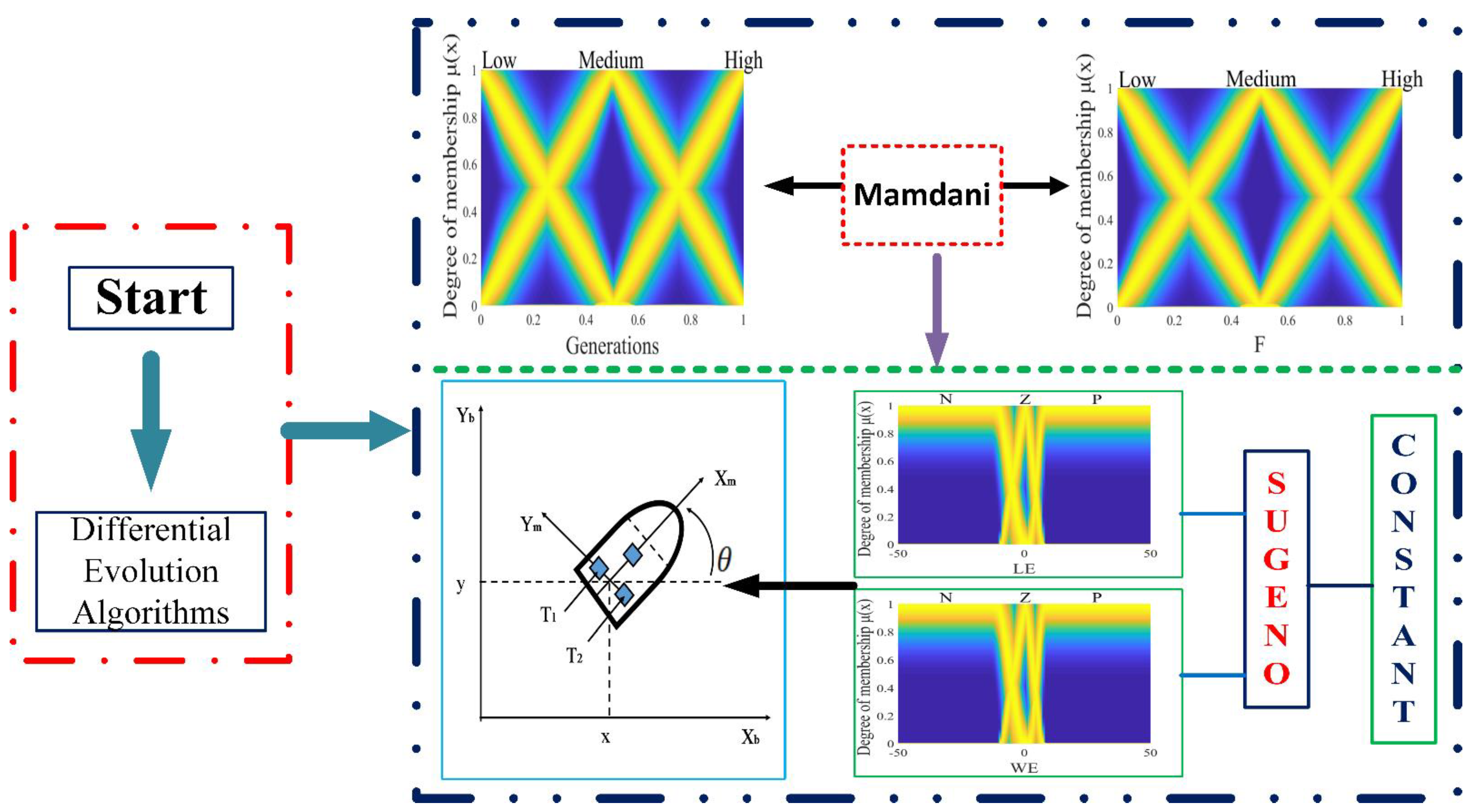
• R1: If generation is low, then F is high;
• R2: If generation is medium, then F is medium;
• R3: If generation is high, then F is low.

Figure 2 shows the surface of the GT2FS.

5. General Type 2 Fuzzy Controller

Recently, one of the most used control cases to test the efficiency of some method has been that of trajectory-following of a mobile robot [37]. The mathematical model of this robot can be found in [38,39]. In this article, the implementation of a general type 2 controller was utilized to test the efficiency of the GT2FDE method, with the aim of validating its performance. Figure 3 represents a graphical illustration of the mobile robot model.

The operation of the robot model is determined by Equations (27) and (28):

$$M\left(q\right)\dot{v}+C\left(q,\dot{q}\right)v+Dv= \mathsf{\tau }+\mathrm{P}\left(\mathrm{t}\right)$$

(27)

where

$\mathrm{q}={\left(\mathrm{x},\mathrm{y}, \mathsf{\theta }\right)}^{\mathrm{T}}$ is the vector of the configuration coordinates;

$\mathrm{v}={\left(\mathrm{v},\right)}^{\mathrm{T}}$ is the vector of velocities;

$\mathsf{\tau }=\left({\mathsf{\tau }}_{1,}{\mathsf{\tau }}_2\right)$ is the vector of the torques applied to the wheels of the robot where ${\tau }_1$ and ${\tau }_2$ denote the torques of the right wheel and the left wheel, respectively;

$P\in R^2$ is the uniformly bounded disturbance vector;

$M\left(q\right)\in R^{2\times 2}$ is the positive–definite inertia matrix;

$C\left(q,\dot{q}\right)\vartheta$ is the vector of centripetal and Coriolis forces;

$D \in R^{2\times 2}$ is a diagonal positive-definite damping matrix.

The kinematic system is determined by Equation (28):

$$\dot{q}=\left[\begin{array}{cc}\cos \theta & 0\\ \sin \theta & 0\\ 0& 1\end{array}\right]\left[\begin{array}{c}v\\ \omega \end{array}\right]$$

(28)

where (x,y) is the position in the $X-Y$ (world) reference frame, $\theta$ is the angle between the heading direction and the x-axis, and $v \mathrm{and} \omega$ are the linear and angular velocities, respectively.

Equation (29) shows the parametrization of a trapezoidal primary generalized type 2 MF with a Gaussian secondary MF ($trapagausstype2$): the $a_1$, $b_1, c_1$, and $d_1$ parameters are for the upper MFs, and $a_2$, $b_2$, $c_2$, and $d_2$ are for the lower MFs:

$$\begin{gathered} \mu \left(x,u\right)=trapagausstype2\left(x,u,\left[a_1,b_1,c_1,d_1,a_2,b_2,c_2,d_2,\alpha ,\rho \right]\right) \\ \mu \left(x,u\right)=exp\left[-\frac{1}{2}{\left(\frac{u-p_x}{{\sigma }_u}\right)}^2\right], \\ \mathrm{where} \\ {\mu }_1\left(x\right)=max\left(min\left(\frac{x-a_1}{b_1-a_1},1,\frac{d_1-x}{d_1-c_1}\right) ,0\right) \\ {\mu }_2\left(x\right)=max\left(min\left(\frac{x-a_2}{b_2-a_2},1,\frac{d_2-x}{d_2-c_2}\right) ,0\right) \\ \overline{\mu }\left(x\right)=\{\begin{array}{cc}max\left({\mu }_1\left(x\right),{\mu }_2\left(x\right)\right)& \forall x\notin \left(b1,c2\right)\\ 1& \forall x\in \left(b1,c2\right)\end{array} \\ \underset{\_}{\mu }\left(x\right)=min\left(\alpha ,min\left({\mu }_1\left(x\right),{\mu }_2\left(x\right)\right)\right) \\ {p}_x=max\left(min\left(\frac{x-a_x}{b_x-a_x},1,\frac{d_x-x}{d_x-c_x}\right) ,0\right), \\ \mathrm{where} a_x=\frac{a_1+a_2}{2}, b_x=\frac{b_1+b_2}{2}, c_x=\frac{c_1+c_2}{2}, d_x=\frac{d_1+d_2}{2} \\ \delta =\overline{\mu }\left(x\right)-\underset{\_}{\mu }\left(x\right) \\ {\sigma }_u=\frac{1+\rho }{2\sqrt{3}}\delta +\epsilon \end{gathered}$$

(29)

where $\rho$ is the fraction of uncertainty of the support secondary membership function.

The general type 2 fuzzy controller (GT2FC) for this problem is a Sugeno system, and it is made up of two antecedents, the linear error (LE) which is observed in Figure 4 and the angular error (WE) which is observed in Figure 5, where the linguistic variables of the antecedents are granulated into negative, zero, and positive linguistic values (N, Z, P). The consequents of this controller consist of constant values, which are identified as torque 1 (T1), which is observed in Figure 6, and torque 2 (T2), which is observed in Figure 7.

The parameters for the GT2MF construction of antecedents are presented in

Table 2. GT2MF antecedent parameters.

LE
GT2MF	${\mathit{a}}_{\mathbf{1}}$	${\mathit{b}}_{\mathbf{1}}$	${\mathit{c}}_{\mathbf{1}}$	${\mathit{d}}_{\mathbf{1}}$	${\mathit{a}}_{\mathbf{2}}$	${\mathit{b}}_{\mathbf{2}}$	${\mathit{c}}_{\mathbf{2}}$	${\mathit{d}}_{\mathbf{2}}$	$\mathbf{\alpha }$	$\mathbf{\rho }$
N	−50	−50	−15	−5	−50	−50	−5	3	0.7	1
Z	−10	−2	6	–	−8	3	8	–	–	2
P	0	5	50	50	5	10	50	50	0.7	1
WE
GT2MF	${\mathit{a}}_{\mathbf{1}}$	${\mathit{b}}_{\mathbf{1}}$	${\mathit{c}}_{\mathbf{1}}$	${\mathit{d}}_{\mathbf{1}}$	${\mathit{a}}_{\mathbf{2}}$	${\mathit{b}}_{\mathbf{2}}$	${\mathit{c}}_{\mathbf{2}}$	${\mathit{d}}_{\mathbf{2}}$	$\mathit{\alpha }$	$\mathit{\rho }$
N	−50	−50	−15	−5	−50	−50	−5	3	0.7	1
Z	−10	−2	6	–	−8	3	8	–	–	2
P	0	5	50	50	5	10	50	50	0.7	1

.

In the consequents, the values of the variables are constant: −50, 0, and 50 for N, Z, and P, with the fuzzy rules presented as follows:

• R1: If the LE is N and WE is N, then T1 is −50 and T2 is −50.
• R2: If the LE is N and WE is Z, then T1 is −50 and T2 is 0.
• R3: If the LE is N and WE is P, then T1 is −50 and T2 is 50.
• R4: If the LE is Z and WE is N, then T1 is 0 and T2 is −50.
• R5: If the LE is Z and WE is Z, then T1 is 0 and T2 is 0.
• R6: If the LE is Z and WE is P, then T1 is 0 and T2 is 50.
• R7: If the LE is P and WE is N, then T1 is 50 and T2 is −50.
• R8: If the LE is P and WE is Z, then T1 is 50 and T2 is 0.
• R9: If the LE is P and WE is P, then T1 is 50 and T2 is 50.

The plant model of the mobile robot used for the experimentation is shown in Figure 8.

The GT2FDE method was used to test the efficiency of the general type 2 fuzzy controller. The configuration of the GT2FDE algorithm parameters used in the experimentation are as follows: CR parameter at 0.5, population of 45, number of simulations is 30, 100 generations.

To test the performance index of the GT2FC controller, simulations were performed without disturbances and with disturbances in the controller. The following

Table 3. Types of disturbances applied to the controller.

Disturbance Number	Type of Disturbance	Configuration of the Parameters
1	Uniform random number	0.05
2	Band-limited white	0.1
3	Pulse-generated	1, 1, 5, and 0

indicates the types of disturbances and the configurations of the used parameters.

The performance index used for the simulations are those presented in the following Equations (30)–(35):

$$ITAE=\sum _{t=1}^{N}t\left(x\left(t\right)-\widehat{x}\left(t\right)\right)$$

(30)

$$ITSE=\sum _{t=1}^{N}t\left({(x\left(t\right)-\widehat{x}\left(t\right))}^2\right)$$

(31)

$$IAE=\sum _{t=1}^N|x\left(t\right)-\widehat{x}\left(t\right)|$$

(32)

$$ISE=\sum _{t=1}^N|{(x\left(t\right)-\widehat{x}\left(t\right))}^2|$$

(33)

$$RMSE=\sqrt{\frac{1}{N} \sum _{t=1}^N{\left(x_t-{\widehat{x}}_t\right)}^2}$$

(34)

$$MSE=\frac{1}{n} \sum _{i=1}^n{({\underset{\_}{Y}}_i-Y_i)}^2$$

(35)

Table 4. Performance index results without disturbance.

Performance Index	LE DE	WE DE	LE GT2FC	WE GT2FC
ITAE	$1.53\times {10}^2$	$1.79\times {10}^1$	$2.16\times {10}^0$	$1.50\times {10}^2$
ITSE	$3.55\times {10}^1$	$5.15\times {10}^{-01}$	$7.61\times {10}^{-01}$	$3.51\times {10}^1$
IAE	$6.49\times {10}^0$	$1.77\times {10}^0$	$1.84\times {10}^0$	$6.34\times {10}^0$
ISE	$2.32\times {10}^0$	$1.38\times {10}^0$	$1.24\times {10}^0$	$2.13\times {10}^0$
RMSE	$2.98\times {10}^0$	$2.98\times {10}^0$	$2.82\times {10}^0$	$2.82\times {10}^0$
MSE	$8.90\times {10}^0$	$8.88\times {10}^0$	$7.94\times {10}^0$	$7.96\times {10}^{-02}$
Execution time	12,227.514 s		12,592.143 s

summarizes the simulations without applying disturbance to the GT2FC, LE and WE DE both use a fixed value of F of 0.5 and a GT2FC.

Figure 9, Figure 10, Figure 11 and Figure 12, the pink color indicates the desired reference signal and the blue color represents the obtained signal.

Figure 9 represents the trajectories of the LE and the WE, without considering disturbances in the controller, of the best result obtained in the experiment, where it can be seen that the trajectories for the LE and the WE are very close to the desired trajectories.

Table 5. Simulations obtained applying one, two, and three disturbances, respectively.

	1		2		3
Performance Index	LE GT2FC	WE GT2FC	LE GT2FC	WE GT2FC	LE GT2FC	WE GT2FC
ITAE	$1.79\times {10}^1$	$1.53\times {10}^2$	$7.01\times {10}^2$	$6.55\times {10}^2$	$4.24\times {10}^1$	$1.60\times {10}^2$
ITSE	$5.15\times {10}^{-1}$	$3.55\times {10}^2$	$6.31\times {10}^2$	$2.93\times {10}^1$	$3.15\times {10}^0$	$3.83\times {10}^1$
IAE	$1.77\times {10}^0$	$6.49\times {10}^0$	$2.88\times {10}^1$	$1.17\times {10}^0$	$2.68\times {10}^0$	$6.78\times {10}^0$
ISE	$1.38\times {10}^0$	$2.32\times {10}^0$	$2.67\times {10}^1$	$1.70\times {10}^{-01}$	$1.47\times {10}^0$	$2.42\times {10}^0$
RMSE	$2.98\times {10}^0$	$2.98\times {10}^0$	$3.44\times {10}^0$	$4.40\times {10}^{-01}$	$2.94\times {10}^0$	$2.94\times {10}^0$
MSE	$8.88\times {10}^0$	$8.90\times {10}^0$	$1.18\times {10}^1$	$6.70\times {10}^{-01}$	$8.65\times {10}^0$	$8.65\times {10}^0$
Execution time	23,134.33 s		36,826.203 s		7067.877 s

shows the simulation results with different disturbances affecting the controller as well as the different errors that were calculated in the experimentation.

Figure 10 shows the best result of the trajectories obtained for the LE and the WE when using disturbance 1; for the LE, it was observed that the trajectory had a small separation from the desired line, while the WE was closer to the desired line.

In the case of disturbance 2, the best trajectories obtained for the LE and the WE are presented in Figure 11, in which we can note that this type of disturbance generates a variation between the desired line and the one obtained for both trajectories.

Finally, the trajectories of the LE and the WE for disturbance 3 are represented in Figure 12. In this case, it was observed that they had a small variation with respect to the desired line.

Regarding the results presented in Table 3 and Table 4, the different errors show that it is possible to obtain stability in the LE and WE trajectories for the different types of disturbances applied to the controller. It is also observed that the different metrics used showed stability in terms of their values, which is corroborated by Figure 10, Figure 11 and Figure 12.

6. Conclusions

The present work shows generalized type 2 fuzzy logic being utilized to dynamically modify the F parameter in differential evolution. In the same way, a robot controller was implemented with a generalized type 2 fuzzy system. In fact, we can highlight this as the main contribution of this article since there is no similar work in the literature regarding the differential evolution algorithm.

Regarding the results presented in Table 4 and Table 5, the different errors show that it is possible to obtain stability in the LE and WE trajectories in the different disturbances applied to the controller. The analysis for the metrics is explained below. In the case of the ITAE metric, it can be observed that the damping of the controller for the different applied disturbances is in the same order. ITSE has the characteristic that when faced with a unit step type input, the response has a large initial error given that it has a small weight, and it can be observed that the results obtained vary with respect to the LE and the WE, where it is observed that the LE has lower values in disturbances 1 and 2. The IAE performance index is not easy to evaluate; however, it is observed in the results they were of the same order, and we could consider them as good. ISE is one of the most important metrics to evaluate a controller. In this case, our results show that for the three disturbances as well as the controller without a disturbance, we had a good performance because it is possible to minimize this performance index. Regarding the RMSE and MSE, all the obtained results were of the same order and indicated that the difference between the desired and obtained lines was minimal, as shown in Figure 10, Figure 11 and Figure 12, where it can be seen that the trajectories for the LE and the WE were very close.

In the future, we plan to consider other kinds of applications [40] and extend the presented approach to type 3 fuzzy logic as has been outlined in [41,42,43,44].

References

1. Sridharan, M. Short review on various applications of fuzzy logic-based expert systems in the field of solar energy. Int. J. Ambient. Energy 2022, 43, 5112–5128. [Google Scholar] [CrossRef]
2. Zhao, L.; Yin, Z.; Yu, K.; Tang, X.; Xu, L.; Guo, Z.; Nehra, P. A Fuzzy Logic Based Intelligent Multi-Attribute Routing Scheme for Two-layered SDVNs. IEEE Trans. Netw. Serv. Manag. 2022, 1. [Google Scholar] [CrossRef]
3. Hosseinpour, S.; Martynenko, A. Application of fuzzy logic in drying: A review. Dry. Technol. 2022, 40, 797–826. [Google Scholar] [CrossRef]
4. Castillo, O.; Castro, J.R.; Melin, P. Type-2 fuzzy logic systems. In Interval Type-3 Fuzzy Systems: Theory and Design; Springer: Cham, Switzerland, 2022; pp. 5–11. [Google Scholar] [CrossRef]
5. Castillo, O.; Melin, P. New Perspectives on Hybrid Intelligent System Design based on Fuzzy Logic. Neural Networks and Metaheuristics; Springer Nature: Cham, Switzerland, 2022; Volume 1050. [Google Scholar]
6. Kaur, J.; Khehra, B.S.; Singh, A. Significance of Fuzzy Logic in the Medical Science. In Computer Vision and Robotics; Springer: Singapore, 2022; pp. 497–509. [Google Scholar] [CrossRef]
7. Quek, S.G.; Selvachandran, G.; Sham, R.; Siau, C.S.; Ramli, M.H.M.; Ahmad, N. A Fuzzy Logic Based Optimal Network System for the Delivery of Medical Goods via Drones and Land Transport in Remote Areas. In International Conference on Intelligent Systems Design and Applications; Springer: Cham, Switzerland, 2022; pp. 1306–1312. [Google Scholar] [CrossRef]
8. Qazi, S.; Iqbal, N.; Raza, K. Fuzzy Logic-Based Hybrid Models for Clinical Decision Support Systems in Cancer. In Computational Intelligence in Oncology; Springer: Singapore, 2022; pp. 201–213. [Google Scholar] [CrossRef]
9. Eckert, J.J.; Barbosa, T.P.; Silva, F.L.; Roso, V.R.; Silva, L.C.; da Silva, L.A.R. Optimum fuzzy logic controller applied to a hybrid hydraulic vehicle to minimize fuel consumption and emissions. Expert Syst. Appl. 2022, 207, 117903. [Google Scholar] [CrossRef]
10. Inozemtsev, A.; Petrochenkov, A.; Kazantsev, V.; Shmidt, I.; Sazhenkov, A.; Dadenkov, D.; Gribkov, I.; Ivanov, P. The Fuzzy Logic in the Problems of Test Control of a Bypass Turbojet Engine Gas Generator. Mathematics 2022, 10, 484. [Google Scholar] [CrossRef]
11. Pan, Y.; Wu, Y.; Lam, H.-K. Security-Based Fuzzy Control for Nonlinear Networked Control Systems with DoS Attacks via a Resilient Event-Triggered Scheme. IEEE Trans. Fuzzy Syst. 2022, 30, 4359–4368. [Google Scholar] [CrossRef]
12. Miranda, M.H.; Silva, F.L.; Lourenço, M.A.; Eckert, J.J.; Silva, L.C. Electric vehicle powertrain and fuzzy controller optimization using a planar dynamics simulation based on a real-world driving cycle. Energy 2022, 238, 121979. [Google Scholar] [CrossRef]
13. Patel, H.R. Fuzzy-based metaheuristic algorithm for optimization of fuzzy controller: Fault-tolerant control application. Int. J. Intell. Comput. Cybern. 2022, 15, 599–624. [Google Scholar] [CrossRef]
14. Boudia, A.; Messalti, S.; Harrag, A.; Boukhnifer, M. New hybrid photovoltaic system connected to superconducting magnetic energy storage controlled by PID-fuzzy controller. Energy Convers. Manag. 2021, 244, 114435. [Google Scholar] [CrossRef]
15. Yang, T.; Sun, N.; Fang, Y. Adaptive Fuzzy Control for a Class of MIMO Underactuated Systems with Plant Uncertainties and Actuator Deadzones: Design and Experiments. IEEE Trans. Cybern. 2022, 52, 8213–8226. [Google Scholar] [CrossRef]
16. Wu, L.; Qian, F.; Wang, L.; Ma, X. An improved type-reduction algorithm for general type-2 fuzzy sets. Inf. Sci. 2022, 593, 99–120. [Google Scholar] [CrossRef]
17. Chen, Y. Study on Weighted-Based Discrete Noniterative Algorithms for Computing the Centroids of General Type-2 Fuzzy Sets. Int. J. Fuzzy Syst. 2022, 24, 587–606. [Google Scholar] [CrossRef]
18. Chen, Y.; Li, C.; Yang, J. Design of Discrete Noniterative Algorithms for Center-of-Sets Type Reduction of General Type-2 Fuzzy Logic Systems. Int. J. Fuzzy Syst. 2022, 24, 2024–2035. [Google Scholar] [CrossRef]
19. Shi, J. A unified general type-2 fuzzy PID controller and its comparative with type-1 and interval type-2 fuzzy PID controller. Asian J. Control. 2022, 24, 1808–1824. [Google Scholar] [CrossRef]
20. Cuevas, F.; Castillo, O.; Cortés-Antonio, P. Generalized Type-2 Fuzzy Parameter Adaptation in the Marine Predator Algorithm for Fuzzy Controller Parameterization in Mobile Robots. Symmetry 2022, 14, 859. [Google Scholar] [CrossRef]
21. Carvajal, O.; Melin, P.; Miramontes, I. Optimal Design and Internet of Things Implementation of a General Type-2 Classifier for Blood Pressure Levels. In International Conference on Intelligent and Fuzzy Systems; Springer: Cham, Switzerland, 2022; pp. 722–729. [Google Scholar] [CrossRef]
22. Ontiveros-Robles, E.; Castillo, O.; Melin, P. Towards asymmetric uncertainty modeling in designing General Type-2 Fuzzy classifiers for medical diagnosis. Expert Syst. Appl. 2021, 183, 115370. [Google Scholar] [CrossRef]
23. Ochoa, P.; Castillo, O.; Melin, P.; Soria, J. Differential Evolution with Shadowed and General Type-2 Fuzzy Systems for Dynamic Parameter Adaptation in Optimal Design of Fuzzy Controllers. Axioms 2021, 10, 194. [Google Scholar] [CrossRef]
24. Mendel, J.M. General type-2 fuzzy logic systems made simple: A tutorial. IEEE Trans. Fuzzy Syst. 2014, 22, 1162–1182. [Google Scholar] [CrossRef]
25. Price, K.V.; Storn, R.M.; Lampinen, J.A. The differential evolution algorithm. In Differential Evolution: A Practical Approach to Global Optimization; Springer: Cham, Switzerland, 2005; pp. 37–134. [Google Scholar]
26. Song, Y.; Cai, X.; Zhou, X.; Zhang, B.; Chen, H.; Li, Y.; Deng, W.; Deng, W. Dynamic hybrid mechanism-based differential evolution algorithm and its application. Expert Syst. Appl. 2023, 213, 118834. [Google Scholar] [CrossRef]
27. Abdelkader, E.M.; Moselhi, O.; Marzouk, M.; Zayed, T. An exponential chaotic differential evolution algorithm for optimizing bridge maintenance plans. Autom. Constr. 2022, 134, 104107. [Google Scholar] [CrossRef]
28. Deng, W.; Ni, H.; Liu, Y.; Chen, H.; Zhao, H. An adaptive differential evolution algorithm based on belief space and generalized opposition-based learning for resource allocation. Appl. Soft Comput. 2022, 127, 109419. [Google Scholar] [CrossRef]
29. Akhtar, M.; Manna, A.K.; Duary, A.; Bhunia, A.K. A hybrid tournament differential evolution algorithm for solving op-timisation problems and applications. Int. J. Oper. Res. 2022, 45, 300–343. [Google Scholar] [CrossRef]
30. Kharchouf, Y.; Herbazi, R.; Chahboun, A. Parameter’s extraction of solar photovoltaic models using an improved differential evolution algorithm. Energy Convers. Manag. 2021, 251, 114972. [Google Scholar] [CrossRef]
31. Zeng, Z.; Zhang, M.; Zhang, H.; Hong, Z. Improved differential evolution algorithm based on the sawtooth-linear population size adaptive method. Inf. Sci. 2022, 608, 1045–1071. [Google Scholar] [CrossRef]
32. De Athayde Prata, B.; Rodrigues, C.D.; Framinan, J.M. A differential evolution algorithm for the customer order scheduling problem with sequence-dependent setup times. Expert Syst. Appl. 2022, 189, 116097. [Google Scholar] [CrossRef]
33. Castillo, O.; Valdez, F.; Soria, J.; Yoon, J.H.; Geem, Z.W.; Peraza, C.; Ochoa, P.; Amador-Angulo, L. Optimal Design of Fuzzy Systems Using Differential Evolution and Harmony Search Algorithms with Dynamic Parameter Adaptation. Appl. Sci. 2020, 10, 6146. [Google Scholar] [CrossRef]
34. Ochoa, P.; Castillo, O.; Soria, J. Differential evolution algorithm using a dynamic crossover parameter with fuzzy logic applied for the CEC 2015 benchmark functions. In North American Fuzzy Information Processing Society Annual Conference; Springer: Cham, Switzerland, 2018; pp. 580–591. [Google Scholar] [CrossRef]
35. Ochoa, P.; Castillo, O.; Soria, J. Interval type-2 fuzzy logic dynamic mutation and crossover parameter adaptation in a fuzzy differential evolution method. In Intuitionistic Fuzziness and Other Intelligent Theories and Their Applications; Springer: Cham, Switzerland, 2018; pp. 81–94. [Google Scholar] [CrossRef]
36. Ochoa, P.; Castillo, O.; Soria, J. Differential Evolution Using Fuzzy Logic and a Comparative Study with Other Metaheuristics. In Nature-Inspired Design of Hybrid Intelligent Systems; Springer: Cham, Switzerland, 2017; pp. 257–268. [Google Scholar] [CrossRef]
37. Peraza, C.; Ochoa, P.; Castillo, O.; Geem, Z.W. Interval-Type 3 Fuzzy Differential Evolution for Designing an Interval-Type 3 Fuzzy Controller of a Unicycle Mobile Robot. Mathematics 2022, 10, 3533. [Google Scholar] [CrossRef]
38. Fukao, T.; Nakagawa, H.; Adachi, N. Adaptive tracking control of a nonholonomic mobile robot. IEEE Trans. Robot. Autom. 2000, 16, 609–615. [Google Scholar] [CrossRef]
39. Martinez, R.; Rodriguez, A.; Castillo, O.; Melin, P.; Aguilar, L.T. Optimization of type-2 fuzzy logic con-trollers for mobile robots using evolutionary methods. In Proceedings of the 2009 IEEE International Conference on Systems, Man and Cybernetics, San Antonio, TX, USA, 11–14 October 2009; pp. 4764–4769. [Google Scholar]
40. Melin, P.; Urias, J.; Solano, D.; Soto, M.; Lopez, M.; Oscar Castillo, O. Voice Recognition with Neural Networks, Type-2 Fuzzy Logic and Genetic Algorithms. Eng. Lett. 2006, 13, 108–116. [Google Scholar]
41. Castillo, O.; Castro, J.R.; Melin, P. Interval Type-3 Fuzzy Control for Automated Tuning of Image Quality in Televisions. Axioms 2022, 11, 276. [Google Scholar] [CrossRef]
42. Castillo, O.; Castro, J.R.; Melin, P. Interval Type-3 Fuzzy Systems: Theory and Design. Stud. Fuzziness Soft Comput. 2022, 418, 1–100. [Google Scholar]
43. Mohammadzadeh, A.; Castillo, O.; Band, S.S.; Mosavi, A. A Novel Fractional-Order Multiple-Model Type-3 Fuzzy Control for Nonlinear Systems with Unmodeled Dynamics. Int. J. Fuzzy Syst. 2021, 23, 1633–1651. [Google Scholar] [CrossRef]
44. Castillo, O.; Melin, P. Towards Interval Type-3 Intuitionistic Fuzzy Sets and Systems. Mathematics 2022, 10, 4091. [Google Scholar] [CrossRef]
Figure 1. Diagram of the general proposal with general type 2 fuzzy systems for controlling a mobile robot and a performance comparison with interval type 2 and type 1 fuzzy systems.
Axioms 12 00156 g001
Figure 2. Surface of the GT2FS.
Axioms 12 00156 g002
Figure 3. Illustration of the mobile robot model.
Axioms 12 00156 g003
Figure 4. Antecedent of the GT2FC.
Axioms 12 00156 g004
Figure 5. Antecedent of the GT2FC.
Axioms 12 00156 g005
Figure 6. Consequent of the GT2FC.
Axioms 12 00156 g006
Figure 7. Consequent of the GT2FC.
Axioms 12 00156 g007
Figure 8. GT2FC of the mobile robot.
Axioms 12 00156 g008
Figure 9. Representation of the best result representing the LE and the WE.
Axioms 12 00156 g009
Figure 10. Representation of the best result representing the LE and the WE.
Axioms 12 00156 g010
Figure 11. Representation of the best result representing the LE and the WE.
Axioms 12 00156 g011
Figure 12. Representation of the best result representing the LE and the WE.
Axioms 12 00156 g012