Dynamic Timed Automata for Reconfigurable System Modeling and Verification

Abstract

Modern discrete-event systems (DESs) are often characterized by their dynamic structures enabling highly flexible behaviors that can respond in real time to volatile environments. On the other hand, timed automata (TA) are powerful tools used to design various DESs. However, they lack the ability to naturally describe dynamic-structure reconfigurable systems. Indeed, TA are characterized by their rigid structures, which cannot handle the complexity of dynamic structures. To overcome this limitation, we propose an extension to TA, called dynamic timed automata (DTA), enabling the modeling and verification of reconfigurable systems. Additionally, we present a new algorithm that transforms DTA into semantic-equivalent TA while preserving their behavior. We demonstrate the usefulness and applicability of this new modeling and verification technique using an illustrative example.

1. Introduction

In recent years, dynamic-structure systems such as cloud computing [1,2], smart grids [3], Industry 4.0 [4,5], and the Internet of things [6] have gained much attention. The design of these highly complex systems is a hot topic, yet it remains a challenging issue that requires suitable and rigorous frameworks [7].

As an intuitive model-checking technique, timed automata [8] (TA) have also found a wide range of applications in the modeling and verification of discrete-event systems (DESs). Several works have used timed automata and their toolbox UPPAAL [9,10,11] as a modeling and simulation environment [12,13,14,15,16]. However, with the significant development of technologies in recent reconfigurable DESs, state-transition systems such as TA and Petri nets [17] exhibit several shortcomings in the design of these modern systems. They do not enable dynamic structure modeling due to their static structure. To address this issue, many researchers have introduced graph transformation systems (GTSs) into state-transition systems to enable their structures to be dynamic [18,19,20,21]. GTSs are well suited for designing complex dynamic systems; however, their high expressiveness impairs any automatic analysis due to their undecidability property. To the best of our knowledge, there is no literature that introduces GTSs into TA to model dynamic structures.

In this paper, we propose a new formalism, called dynamic timed automata (DTA), which allows the modeling and verification of dynamic-structure DESs by handling dynamic typologies in TA. We also provide a new algorithm that transforms DTA into semantically equivalent TA, which unfolds reachable configurations of a given DTA into a basic TA that preserves the original behavior. This enables a model-checking process to be carried out using analysis methods supported by off-the-shelf tools, such as UPPAAL. It is important to note that the proposed approach focuses on the properties of a reconfigurable system under consideration and does not involve the verification of GTSs themselves. For instance, a critical pair analysis (CPA) [22], used to detect dependencies and conflicts between transformation rules, is not considered since it is beyond the scope of this research. Nevertheless, as suggested in [23], a CPA can assist a designer in detecting dependencies or conflicts by using existing tools (e.g., AGG [24]). The designer can then modify the models or keep the conflicts and dependencies. After resolving these issues, the designer can apply the GTS to a TA modeling an initial configuration to obtain the set of all possible configurations.

The remainder of this paper is organized as follows. An overview of some related works is provided in Section 2. Section 3 recalls the necessary basics of TA and graph transformations. Section 4 and Section 5 present the proposed DTA formalism and its unfolding towards TA. The semantic equivalence between any given DTA and its unfolding towards TA is proven in Section 6. Section 7 exploits the proposed formalism to design a reconfigurable system. Finally, Section 8 concludes the paper.

2. Related Work

In the literature, an extensive amount of research has used timed automata to model and verify various kinds of real-time systems [12,13,14,15,16]. The automated consistency checks of the reconfiguration steps of dynamic software product lines (DSPLs) were facilitated in [25] by translating real-time requirements into TA. To improve the performance of consistency checks for DSPL specifications based on TA, different static-analysis techniques were combined in [26]. To guarantee the consistency of resource delivery in a cloud service, the authors of [27] used UPPAAL for the modeling and verification of clients, service managers, and resource services to offer a framework of resource provisioning as a service in the cloud. To handle the dynamics of reputation, the authors in [28] designed a calculus of mobile agents to cope with such features and then encoded them into networks of weighted TA.

Timed automata have been adapted to various formalisms to tackle different challenges. One such adaptation is parametric timed automata (PTA) [29], which allows for more realistic timing constraints. For instance, a constraint that states “an action X must occur within the time it takes to execute n actions Y” is more realistic than a constraint that states “an action X must occur within m milliseconds”. This allows the creation of specifications that are based on certain parameters of the environment in which a system operates. Studies in [29,30] found that the problem of determining whether a certain state was reachable was decidable in two scenarios: when using PTA with a single parametric clock, and when using PTA with two parametric clocks and a single parameter. However, the problem of determining reachability was undecidable when using PTA with three or more parametric clocks.

Cordy et al. [31] proposed featured timed automata (FTA) to model and verify the variability in software product lines (SPLs). In FTA, clock constraints on switches and locations were annotated with feature constraints. Hence, instead of considering every product variant one-by-one during the verification process (which is infeasible), entire product lines could be verified in a single run. Although FTA provided a powerful tool, their expressiveness only allowed Boolean feature constraints. To enable unbounded timing intervals of real-time constraints in FTA, Luthmann et al. [32] defined configurable PTA (CoPTA) combining FTA and PTA. However, due to their nature, CoPTA potentially comprised an infinite number of TA model variants. Thus, a variant-by-variant analysis strategy for CoPTA was impossible. To tackle this issue, Luthmann et al. [33] adapted a family-based test-suite generation methodology presented in [34] to CoPTA models.

Latreche and Belala [35] developed a new type of timed automata called recursive and dynamic timed automata (RDTA) which allowed the automata to be recursively invoked by other automata. These were used to analyze and specify procedures for recovering from failures and updating partner services in dynamic Web service compositions. Another formalism, called dynamic networks of timed automata (DNTA), was introduced in [36] to allow for the creation and destruction of multiple copies of automata at runtime for modeling complex systems. In [37], the authors presented dynamic input/output automata (DIOA) which allowed the dynamic creation, destruction, and changes in the signature of an automaton. The works provided in [38,39] described an extension of TA, called reconfigurable hierarchical TA (RHTA), which involved manually constructing all reachable configurations and incorporating them into a single model which could often lead to cumbersome models. Moreover, a reconfiguration in RHTA was expressed by a simple switching between configurations.

Although the cited extensions are considered practical, provide a certain degree of flexibility in the modeling, and enhance the expressiveness of TA, they cannot model or verify dynamic-structure automata. For instance, FTA and CoPTA can model variability in SPLs; however, each variant is static and cannot change its structure. As for RDTA, they can only specify and analyze the backward recovery procedures and the update of partner services in case of failure; thus, neither new structures nor other behaviors are allowed. Even though DNTA and DIOA enable dynamic sets of automata by instantiating or destroying them, the structure of any automaton remains static. Furthermore, DIOA are based on untimed automata, and they can only exhibit or hide certain behaviors without allowing the introduction of new ones. Finally, RHTA represent reconfigurations by static models, which can only make the modeling process laborious at best, therefore losing the benefits of a direct representation [37].

The formalism proposed in this paper outperforms the above-mentioned extensions in several ways:

• It enables the separation of concerns by modeling dynamic structures using GTSs, which explicitly model system features and component set evolution at two separate levels [40];
• It provides an unfolding algorithm that transforms DTA to semantic-equivalent TA, thereby making the design and verification of dynamic systems more efficient by reusing the existing TA tools in the analysis of DTA;
• All properties that are decidable in the TA formalism remain decidable in the new extension, since any given DTA can be unfolded to a plain TA that preserves the behavior of its original DTA.

3. Preliminaries

This section outlines the necessary basics of the formalisms exploited in this work.

3.1. Timed Automata

Timed automata (TA) [8] extend finite automata by introducing real-valued clocks to accept timed languages. Let C be a set of clocks. For each clock $x\in C$, the following is considered:

• Initially, the value of x is zero;
• Its value increases simultaneously with other clocks by the same speed;
• It can be reset to zero with any edge.

Let $\mathcal{G}\left(C\right)$ be the set of conjunctive formulae of atomic constraints built over C of the form $x\bowtie a$ or $x-y\bowtie a$, where $x,y\in C$, $\bowtie \in \{<,\le ,=,\ge ,>\}$, and $a\in \mathbb{N}$. The formal definition of a timed automaton is provided as follows.

Definition 1.

(Timed automaton). A TA A is a tuple $⟨S,s_0,\Sigma ,C,E,I⟩$ where:

(1)

S is a nonempty finite set of locations;

(2)

$s_0$ ⊂ S is a set of initial locations;

(3)

Σ is a finite set of actions containing an internal action denoted by τ;

(4)

C is a finite set of clocks;

(5)

$E\subseteq S\times \Sigma \times \mathcal{G}\left(C\right)\times 2^C\times S$ is a set of edges between locations, where $(s,\sigma ,g_c,\delta ,s^{\prime })\in E$ means the following;

(a)

s and $s^{\prime }$ are the source and the target locations, respectively;

(b)

σ is an action;

(c)

$g_c$ is an enabling condition built over C;

(d)

$\delta \subseteq C$ is a subset of clocks to be reset.

(6)

$I:S\to \mathcal{G}\left(C\right)$ assigns invariants to locations.

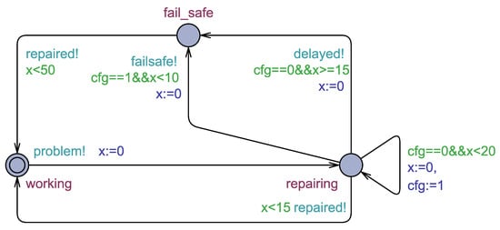
Example 1.

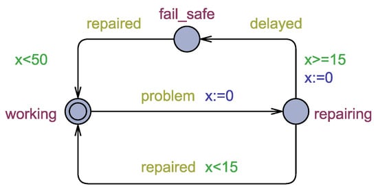
Consider a TA A depicted in Figure 1 that models a system with three states: working, repairing, and fail_safe. Initially, A is in its initial location working depicted by a double circle. When a problem arises, the automaton changes its location to repairing and resets clock x (i.e.,x:=0). At location repairing, the system should be repaired within 15 time units. If the system is repaired before the deadline, it returns to its initial state working. If not, it changes its state to fail_safe mode and resets clock x. Finally, after entering fail_safe, any breakdown must be repaired before 50 time units have passed, after which A returns to location working.

Figure 1. A TA modeling a system having three states.

UPPAAL increases the expressiveness of TA by introducing constants, discrete local/global variables, and the communication channels [11] used by automata to communicate with each other. Indeed, a set of automata communicating on (shared) global variables and channels constitutes a global context called a network of TA (NTA).

For an NTA composed of a set of automata, a set of synchronized channels $\mathtt{Chan}$, and a set of global variables ${\mathtt{V}}^{\mathtt{g}}$, consider the following.

• Let $\mathtt{Sync}=\{\mathtt{c}!,\mathtt{c}?\mid \mathtt{c}\in \mathtt{Chan}\}\cup \{-\}$ be a set of synchronizations, such that c! and c? represent the initiation and the acceptance, respectively, of synchronization over channel c, and “−” stands for no synchronization.
• Let $\mathtt{V}={\mathtt{V}}^{\mathtt{g}}\cup {\mathtt{V}}^{\mathtt{l}}$ be a set of variables.
• Let $\mathtt{Guards}\left(\mathtt{V}\right)$ be the set of logical conditions built over $\mathtt{V}$.
• Let $\mathtt{Exp}\left(\mathtt{V}\right)$ be the set of expressions built over $\mathtt{V}$.
• Let $\mathtt{Assign}\left(\mathtt{V}\right)$ be the set of finite sequences of assignments of the form $\mathtt{v}:=\mathtt{exp}$, where $\mathtt{v}\in \mathtt{V}$ and $\mathtt{exp}\in \mathtt{Exp}\left(\mathtt{V}\right)$.

Definition 2.

(Timed automaton in UPPAAL).A TA in UPPAAL is a tuple ⟨V^l, $S,s_0,\Sigma ,C,E,I⟩$ such that:

(1)

V^l is a set of initialized local variables (a variable in UPPAAL can be a real or an integer);

(2)

$S,s_0,\Sigma ,C$, and I are as in Definition 1;

(3)

$E\subseteq S\times \Sigma \times \mathcal{G}\left(C\right)\times$  Guards(V) × Sync × 2^c × Assign(V) × S is a set of edges, where for $e=(s,\sigma ,g_c,g_v,z,\delta ,\alpha ,s^{\prime })\in E$:

(a)

$s,\sigma ,g_c,\delta$, and $s^{\prime }$ are as provided in Definition 1;

(b)

$g_v$ is an enabling condition built over V;

(c)

z is a synchronization on a channelc. Note that the synchronization can take place only if an edge e of automaton A is sending on c (i.e., c!) and an edge $e^{\prime }$ of automaton $A^{\prime }$ is receiving on c (i.e., c?);

(d)

α is a sequence of assignments updating the values of variables in V.

Example 2.

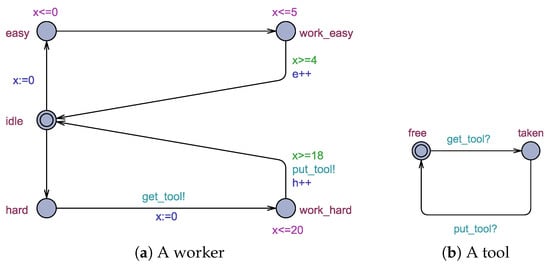
Consider a network of timed automata shown in Figure 2. This NTA models a job shop (inspired by [10]) consisting of workers (see Figure 2a) and tools (see Figure 2b). In this job shop, workers share certain tools to manufacture products from simple components. A worker picks up some components and decides whether to perform an easy task with their hands, i.e., no tool is involved, or a hard task using an available tool.

Figure 2. A network of timed automata modeling a job shop.

Initially, each worker is in locationidleand each tool is in locationfree. If a worker decides to perform an easy task, they start working on it straightaway. This behavior is modeled by moving from locationidleto locationeasyand then to locationwork_easy. The invariant “x<=0” associated with locationeasymodels that a worker needs no time to start an easy task. In addition, the invariant “x<=5” associated with location work_easy means that an easy task is performed at most in five time units. After finishing an easy task, a global variable called “e” (the number of finished easy tasks) is incremented.

As for hard tasks, moving from locationhardto locationwork_hardrequires the existence of an available tool. This is modeled by both synchronizations “get_tool!” and “get_tool?” shown in Figure 2a,b, respectively. That is, a worker automaton sending on channel “get_tool” can move from locationhardtowork_hardiff there is a tool automaton receiving on “get_tool”. Finally, after finishing a hard task, a global variable called “h” (the number of finished hard tasks) is incremented and the synchronization on channel “put_tool” is initiated.

3.2. Graph Transformation: A Double-Pushout Approach

In this work, the reconfiguration of timed automata is modeled based on a widely used graph transformation formalism called double-pushout (DPO) approach. This approach provides a theoretical and suitable framework for modeling dynamic-structure systems in a rigorous way [18].

We start by defining graph morphism, an important concept in graph transformation. It preserves the structure of a graph G in a graph H by mapping nodes of G to nodes of H so that each edge in G must have an image in H.

Definition 3.

(Graph morphism).Let $V_G$ and $E_G$ denote sets of nodes and edges of a graph G, respectively. Let $G=⟨V_G,E_G⟩$ and $H=⟨V_H,E_H⟩$ be two graphs. A function $\phi :V_G\to V_H$ is a graph morphism if the following holds: $\forall (v,w)\in E_G,(\phi \left(v\right),\phi \left(w\right))\in E_H$.

In DPO, a transformation is provided as a rule $r=L\stackrel{{\phi }_l}{\leftarrow }I\stackrel{{\phi }_r}{\to }R$ consisting of three graphs L, I, and R and two graph morphisms ${\phi }_l$ and ${\phi }_r$, where:

• L is a left-hand side (to be removed);
• I is a common interface;
• R is a right-hand side (to be inserted);
• ${\phi }_l:I\to L$ is a graph morphism;
• ${\phi }_r:I\to R$ is a graph morphism.

Given a rule r, elements in L that do not belong to the image of ${\phi }_l$ are called obsolete and elements in R that do not belong to the image of ${\phi }_r$ are called fresh. A rule r applies to a graph G if an occurrence (located by a graph morphism m) of its left-hand side L exists in G. If graph morphisms m, ${\phi }_l$, and ${\phi }_r$ are injective, then the obsolete elements of L are removed from G (the obtained graph is called context) and fresh elements of R are added to the context graph, resulting in a new graph H. This transformation is denoted by $G\stackrel{r,m}{\Rightarrow }H$. In this paper, we only considered injective graph morphisms. The DPO-based transformations are also represented by diagrams, as depicted in Figure 3.

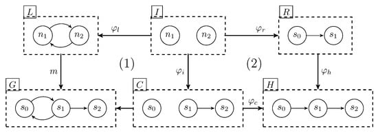
Figure 3. A DPO diagram.

A DPO transformation performs two steps called pushout. Informally, the first pushout (see Box (1) in Figure 3) resolves the existence of a context graph C to be glued (the graph gluing is explained below) with L over I to obtain G, denoted by $G=C{+}_{I}L$. If C exists, then the rule applies to G. The second pushout (see Box (2) in Figure 3) glues C with R over I to yield graph H.

The obtained graph $H=⟨V_H,E_H⟩=C{+}_{I}R$ is defined as follows.

1.

$V_H=V_C\uplus (V_R\backslash V_I)$ (such that “⊎” denotes the disjoint union);

2.

$E_H=E_C\uplus E_R$.

Consider an application of a rule $r=L\stackrel{{\phi }_l}{\leftarrow }I\stackrel{{\phi }_r}{\to }R$ to a graph G shown in Figure 3. The first pushout is performed as follows. A morphism m locates an occurrence of L in G, such that $m\left(n_1\right)=s_0$ and $m\left(n_2\right)=s_1$. Then, a context graph C is defined so that $G=C{+}_{I}L$. Hence, the rule is applicable. In the second pushout, nodes and edges of C and a fresh edge of R (which is $(s_0,s_1)$) are inserted into H.

4. Dynamic Timed Automata

In this paper, we present a new formalism, called dynamic timed automata (DTA), that overcomes the limitations of traditional TA in modeling dynamic-structure reconfigurable systems. We also present a new algorithm that transforms DTA into equivalent TA while preserving their behavior.

This section presents the formal definition of the DPO-based DTA formalism. In the following sections, we develop an algorithm for unfolding DTA into semantic-equivalent TA, and we prove the equivalence between DTA and their unfolding towards TA through the proposed algorithm.

To begin, we extend the definition of graph morphism provided in Definition 3.

Definition 4.

(TA morphism).Let $A_1=⟨{\mathtt{V}}_1^{\mathtt{l}},S_1,s_{01},{\Sigma }_1,C_1,E_1,I_1⟩$ and $A_2=⟨{\mathtt{V}}_2^{\mathtt{l}},S_2,s_{02},{\Sigma }_2,$$C_2,E_2,I_2⟩$ be two TA, where ${\mathtt{V}}_1^{\mathtt{l}}\subset {\mathtt{V}}_2^{\mathtt{l}}$, ${\Sigma }_1\subset {\Sigma }_2$, and $C_1\subset C_2$. A TA morphism $\phi :A_1\to A_2$ is a mapping $\phi :S_1\to S_2$ such that the following hold.

• $\forall s\in S_1$, if $s\in s_{01}$, then $\phi \left(s\right)\in s_{02}.$ (Note that $s_{01}$ might be empty);
• $\forall e_1=(s_1,\sigma ,g_c,g_v,z,\delta ,\alpha ,s_1^{\prime })\in E_1,\exists e_2=(s_2,\sigma ,g_c,g_v,z,\delta ,\alpha ,s_2^{\prime })\in E_2,\phi \left(s_1\right)=s_2$ and $\phi \left(s_1^{\prime }\right)=s_2^{\prime }$;
• $\forall s\in S_1,I_1\left(s\right)=I_2\left(\phi \left(s\right)\right)$.

Definition 5.

(Transformation rules).A transformation rule r is defined as $⟨L\stackrel{{\phi }_l}{\leftarrow }I\stackrel{{\phi }_r}{\to }R,g,u⟩$, such that:

1.

L is a left-hand side TA;

2.

I is a common interface TA;

3.

R is a right-hand side TA, $|S_L|=|S_I|=|S_R|$, such that $S_A$ denotes the location set of A;

4.

${\phi }_l:I\to L$ is a TA morphism;

5.

${\phi }_r:I\to R$ is a TA morphism;

6.

$g=(s,g_c,g_v)$ is a precondition of r such that s is a location and $g_c$ (resp. $g_v$) is an enabling condition built over clocks (respectively, variables);

7.

$u=(\delta ,\alpha )$ is a post-condition (i.e., effect) of r such that δ is a set of clocks to be reset and α is a sequence of assignments.

Moreover, rules that can only modify the set of edges (i.e., topology) of an automaton are considered in this work.

Definition 6.

(Dynamic timed automata).A DTA $\mathcal{D}$ is a pair $⟨A_0,\mathcal{R}⟩$, such that:

1.

$A_0$ is a TA;

2.

$\mathcal{R}$ is a set of transformation rules.

Let A be a TA. A rule $r=⟨L\stackrel{{\phi }_l}{\leftarrow }I\stackrel{{\phi }_r}{\to }R,g,u⟩$ with a match $m:L\to A$ applies to a DTA $\mathcal{D}$ iff:

1.

A is the current configuration of $\mathcal{D}$;

2.

There exists a TA C such that $A=C{+}_{I}L$;

3.

$g=(s,g_c,g_v)$ is satisfied, that is, s is the current location of A, and the valuations of both guards $g_c$ and $g_v$ are true.

After applying $r=⟨L\stackrel{{\phi }_l}{\leftarrow }I\stackrel{{\phi }_r}{\to }R,g,u⟩$ to A, $\mathcal{D}$ changes its configuration towards $A^{\prime }$ such that $A^{\prime }=C{+}_{I}R$.

Example 3.

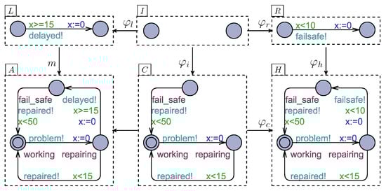
Consider a DTA $\mathcal{D}=⟨A,\left\{r\right\}⟩$, where TA A and rule r are depicted in Figure 4. Rule $r=⟨L\stackrel{{\phi }_l}{\leftarrow }I\stackrel{{\phi }_r}{\to }R,g,u⟩$ is defined as follows:

Figure 4. Reconfiguration via rule r.

1.

L, I, R, ${\phi }_l$ and ${\phi }_r$ are shown in Figure 4;

2.

$g=(s,g_c,g_v)$, such that $s=$repairing, $g_c=$"x < 20"and $g_v=$“true”;

3.

$u=(\delta ,\alpha )$, such that δ = {x} and $\alpha =\epsilon$ (i.e., an empty sequence).

Rule r applies to A, given the following:

• Its precondition g is satisfied (i.e., the current location of A isrepairingand the value of clockxis less than 20);
• A morphism m finds an occurrence of L in A, such that the left and right locations of L are mapped torepairingandfail_safe, respectively;
• There exists a TA C, shown in Figure 4, such that $A=C{+}_{I}L$.

After applying r, the current configuration of $\mathcal{D}$ becomes H illustrated in Figure 4.

5. DTA Transformation towards Basic TA

Timed automata enjoy a variety of tools and frameworks exploited in their design and analysis. This fact motivates the unfolding of DTA into TA. Therefore, the traditional verification tools designed for basic TA can be utilized in the DTA analysis.

In fact, reconfigurations insert and/or remove edges to enable new behaviors/topologies. As a result, any given unfolding of a DTA must model these reconfigurations and their effects. In this context, we developed an algorithm that unfolds any given DTA $\mathcal{D}$ into a semantic-equivalent TA $\mathcal{A}$ according to its shape and behavior.

For a DTA $\mathcal{D}=⟨A_0,\mathcal{R}⟩$, consider the following:

1.

Let $\mathcal{C}=\{A_0,\cdots ,A_n\}$ be a set of TA obtained by applying sequences of rules in $\mathcal{R}$ to $A_0$.

2.

Let $E_i$ be the set of edges in $A_i$.

3.

Let $\mathcal{E}={\bigcup }_{i=0}^n{E}_i$ be a set of edges.

4.

Let $\mathcal{C}\left(e\right)=\{A_i\mid A_i\in \mathcal{C}\mathrm{and}e\in E_i\}$.

5.

Let $\mathcal{T}=\{(A^s,r,A^t)\mid A^s,A^t\in \mathcal{C}\mathrm{and}{A}^s\stackrel{r}{\Rightarrow }{A}^t\}$ be a set of transformations applicable to DTA $\mathcal{D}$, where r is an applicable rule to $\mathcal{D}$, and $A^s,A^t$ are its source and target configurations, respectively.

The intuition of the proposed unfolding algorithm provided in Algorithm 1 that transforms a given DTA $\mathcal{D}$ to a TA $\mathcal{A}$ is given as follows:

1.

Let $A_0=⟨{\mathtt{V}}_0^{\mathtt{l}},S_0,s_{00},{\Sigma }_0,C_0,E_0,I_0⟩$ be an initial configuration of $\mathcal{D}$.

2.

Let $\mathtt{Enum}:\mathcal{C}⟶\{0,\cdots ,n\}$ be an enumeration of configurations $A_0,\cdots ,A_n$ in $\mathcal{C}$ by means of a natural ordering.

3.

Let ${\mathtt{V}}^{\mathtt{l}}\leftarrow {\mathtt{V}}_0^{\mathtt{l}}\cup \left\{\mathtt{cfg}\right\}$, where cfg is a bounded local integer variable (initialized to zero) used to represent the current configuration of $\mathcal{D}$, that is, if $\mathtt{cfg}=\mathtt{i}$ then the current configuration of $\mathcal{D}$ is $A_i$, where $\mathtt{Enum}\left(A_i\right)=\mathtt{i}$.

4.

Let $E⟵\varnothing$.

5.

For each edge $e\in \mathcal{E}$ that is present in every configuration in $\mathcal{C}$, i.e., $\mathcal{C}\left(e\right)=\mathcal{C}$, insert e into E, i.e., $E⟵E\cup \left\{e\right\}$.

6.

For each edge $e=(s,\sigma ,g_c,g_v,z,\delta ,\alpha ,s^{\prime })\in \mathcal{E}$ that does not belong to certain configurations in $\mathcal{C}$, i.e., $\mathcal{C}\left(e\right)⊊\mathcal{C}$, do:

(a)

Build a condition le of the form “cfg==i${}_0$||...||cfg==i${}_{\left|\mathcal{C}\right(e\left)\right|}$” (|| and && stand for “logical or” and “logical and”, respectively), where i${}_0,\cdots ,$i${}_{\left|\mathcal{C}\right(e\left)\right|}$ are the indices, obtained by Enum, of configurations in $\mathcal{C}\left(e\right)$.

(b)

Create $e^{\prime }=(s,\sigma ,g_c,g_v^{\prime },z,\delta ,\alpha ,s^{\prime })$, where $g_v^{\prime }=$“le && $g_v$” (6a).

(c)

Insert $e^{\prime }$ into E, i.e., $E⟵E\cup \left\{e^{\prime }\right\}$.

7.

For each transformation $(A^s,r,A^t)\in \mathcal{T}$, do:

(a)

Let $g=(s,g_c,g_v)$ and $u=(\delta ,\alpha )$ be the pre- and postconditions of rule r.

(b)

Let $g_v^{\prime }=$“cfg==i && $g_v$”, where i = Enum$\left(A^s\right)$.

(c)

Let ${\alpha }^{\prime }=$“$\alpha$,cfg: = j”, where j = Enum$\left(A^t\right)$.

(d)

Create an edge $e=(s,\tau ,g_c,g_v^{\prime },-,\delta ,{\alpha }^{\prime },s)$ (recall that $\tau$ and “−” stand for internal action and no synchronization, respectively).

(e)

Insert e into E, i.e., $E⟵E\cup \left\{e\right\}$.

8.

Let $S\leftarrow S_0$, $s_0\leftarrow s_{00}$, $\Sigma \leftarrow {\Sigma }_0$, $C\leftarrow C_0$, and $I\leftarrow I_0$.

9.

Let $\mathcal{A}=⟨{\mathtt{V}}^{\mathtt{l}},S,s_0,\Sigma ,C,E,I⟩$.

Consider Steps (6) and (7). In fact, the former represents an edge e of $\mathcal{D}$ by an edge $e^{\prime }$ in $\mathcal{A}$, where the condition “le&&$g_v$” enables $e^{\prime }$ only if (i) the current configuration of $\mathcal{A}$ is one of the configurations in which e appears, and (ii) $g_v$, the enabling condition of e, is true. By the latter, the algorithm creates an edge e to represent an application of a rule r to source configuration $A^s$ yielding a target configuration $A^t$, such that: (i) the guards of e are identical to those of r and, in addition, the current configuration is $A^s$ which is expressed by “cfg==i” where cfg is a variable used to represent the current configuration of $\mathcal{D}$ and i is the index of configuration $A^s$; and (ii) the effects (clocks to be reset and variables assignments) of e are identical to those of r, and, in addition, the current configuration becomes $A^t$ which is expressed by “cfg:=j”, where j is the index of configuration $A^t$.

Algorithm 1: DTA transformation towards TA.

Require: $\mathcal{D}=⟨A_0,\mathcal{R}⟩$: DTA

Ensure: $\mathcal{A}=⟨{\mathtt{V}}^{\mathtt{l}},S,s_0,\Sigma ,C,E,I⟩$: TA

1: Initialization:

2: Let $A_0=⟨{\mathtt{V}}_0^{\mathtt{l}},S_0,s_{00},{\Sigma }_0,C_0,E_0,I_0⟩$

3: cfg  $⟵\mathtt{0}$

4: ${\mathtt{V}}^{\mathtt{l}}⟵{\mathtt{V}}_0^{\mathtt{l}}\cup \left\{\mathtt{cfg}\right\}$

5: $⟨S,s_0,\Sigma ,C,I⟩⟵⟨S_0,s_{00},{\Sigma }_0,C_0,I_0⟩$

6: $E⟵\varnothing$

7: Apply rules in $\mathcal{R}$ to $A_0$

8: Compute $\mathcal{T}$

9: Compute $\mathcal{C}$

10: Let $\mathtt{Enum}:\mathcal{C}⟶\{0,\cdots ,n\}$ be an enumeration

11: $\mathcal{E}⟵\varnothing$

12: for each $A_i\in \mathcal{C}$ do

13: $\mathcal{E}⟵\mathcal{E}\cup E_i$

14: end for

15: Represent edges of $\mathcal{D}$ in $\mathcal{A}$:

16: for each $e=(s,\sigma ,g_c,g_v,z,\delta ,\alpha ,s^{\prime })\in \mathcal{E}$ do

17: if $\mathcal{C}\left(e\right)=\mathcal{C}$ then

18:  $E⟵E\cup \left\{e\right\}$

19: else

20:  Pick arbitrarily A from $\mathcal{C}\left(e\right)$

21:  $\mathtt{le}⟵“\mathtt{cfg}==”+\mathtt{Enum}\left(A\right)$

22:  for each $A_i\in \mathcal{C}\left(e\right)\backslash \left\{A\right\}$ do

23:   $\mathtt{le}⟵\mathtt{le}+“\left|\right|\mathtt{cfg}==”+\mathtt{Enum}\left(A_i\right)$

24:  end for

25:  $e^{\prime }⟵(s,\sigma ,g_c,\mathtt{le}\&\&g_v,z,\delta ,\alpha ,s^{\prime })$

26:  $E⟵E\cup \left\{e^{\prime }\right\}$

27: end if

28: end for

29: Represent rules of $\mathcal{R}$ in $\mathcal{A}$:

30: for each $(A^s,r,A^t)\in \mathcal{T}$ do

31: $g_v^{\prime }⟵“\mathtt{cfg}==”+\mathtt{Enum}\left(A^s\right)+“\&\&g_v”$

32: ${\alpha }^{\prime }⟵\alpha +“,\mathtt{cfg}:=”+\mathtt{Enum}\left(A^t\right)$

33: $e⟵(s,\tau ,g_c,g_v^{\prime },-,\delta ,{\alpha }^{\prime },s)$

34: $E⟵E\cup \left\{e\right\}$

35: end for

36: Termination:

37: $\mathcal{A}⟵⟨{\mathtt{V}}^{\mathtt{l}},L,l_0,\Sigma ,C,E,I⟩$

Example 4.

In this example, we applied the unfolding algorithm to DTA $\mathcal{D}$ shown in Figure 4. The resulting TA $\mathcal{A}$ is depicted in Figure 5.

Figure 5. Equivalent TA $\mathcal{A}$ to DTA $\mathcal{D}$.

• In the following, we use the proposed algorithm to create an equivalent TA $\mathcal{A}=⟨$ V^l $,S,s_0,\Sigma ,C,E,I⟩$ to $\mathcal{D}=⟨A,\mathcal{R}⟩$.

• Initialization:First, we start the creation of automaton $\mathcal{A}$ such that its sets of locations, initial locations, actions and clocks, and function I are identical to those in A. Additionally, we add a local variable, called cfg, initialized to zero, to those of A to create a local variable set of $\mathcal{A}$. Thus,

• V^l = {cfg}, where ${\mathtt{V}}_0^{\mathtt{l}}=\varnothing$;
• S = {working, repairing, fail_safe};
• $s_0$ = {working;}
• $\Sigma =\left\{\tau \right\}$;
• $C$ = {x};
• $I:S⟶\left\{\mathrm{true}\right\}$, wheretruemeans there are no invariants on location.

• Second, we apply rules in $\mathcal{R}$ to A to yield two sets: (i) $\mathcal{C}=\{A,H\}$, where configurations A and H are illustrated in Figure 4, and (ii) $\mathcal{T}=\left\{\right(A,r,H\left)\right\}$. Finally, we enumerate the configurations in $\mathcal{C}$ using a natural ordering; hence,Enum$\left(A\right)=0$ andEnum$\left(H\right)=1$.

• Represent edges of $\mathcal{D}$ in $\mathcal{A}$:First, we consider edges in $\mathcal{D}$ that remain unchanged during reconfigurations, i.e., they exist in configurations of $\mathcal{D}$. These edges are:

• e₁ = (working, τ, true, true, problem!, {x}, ε, repairing);
• e₂ = (repairing, τ, “x < 15”, true, repaired!, {x}, ∅, ε, working);
• e₃ = (fail_safe, τ, “x < 50”, true, repaired!, {x}, ∅, ε, working);

• wheretrueindicates “no guards”, and ε denotes “an empty sequences”.

• Consider edges that do not appear in every configuration of $\mathcal{D}$, namely:

• e_A = (repaired, τ, “x >= 15”, true, delayed!, {x}, ε, fail_safe) in A;
• e_H = (repaired, τ, “x < 10”, true, failsafe!, {x}, ε, fail_safe) in H;

• Since edge $e_A$ only belongs to configuration A, i.e., $\mathcal{C}\left(e_A\right)=\left\{A\right\}$, the enabling condition (built over variables) of edge $e_A^{\prime }$, which represents $e_A$ in $\mathcal{A}$, is computed as follows “cfg==0&&true”, wheretrueis the enabling condition of $e_A$ and 0 is the index of configuration A. Thus, $e_A^{\prime }$ = (repairing, τ, “x >= 15”, “cfg==0”, delayed!, {x}, ε, fail_safe). Similarly, $e_H^{\prime }$, which represents $e_H$, is defined as follows: $e_H^{\prime }$ = (repairing, τ, “x < 10”, “cfg==1”, failsafe!, {x}, ε, fail_safe). Finally, edges $e_1$, $e_2$, $e_3$, $e_A^{\prime }$, and $e_H^{\prime }$ are added to set E.

• Adding edges to emulate rules:An application of r to A results in H, where $e_A$ is no longer present and $e_H$ is newly added. In $\mathcal{D}$, r applies under the following conditions: (i) its current configuration is A, (ii) the value of clock x is less than 20, and (iii) the current location of A isrepairing. Hence, the preconditions of edge $e_r$, which represent this application, are (i) “cfg==0” and (ii) “x < 20”; furthermore, (iii) the source and target location of $e_r$ isrepairing. Moreover, when r applies, (a) clockxis reset, and (b) the current configuration of $\mathcal{D}$ is changed to H. Therefore, the postconditions of edge $e_r$ are (a) “x:=0” and (b) “cfg:=1”. Finally, we insert $e_r$ = (repairing, τ, “x < 20”, “cfg==0”, −, “{x}”, “cfg==1”, repairing) into E. Recall that τ and “−” stand for internal action and no synchronization, respectively.

• Termination:Finally, the equivalent TA $\mathcal{A}=⟨$ V^l, $S,s_0,\Sigma ,C,E,I⟩$ to DTA $\mathcal{D}$ is given as follows.

• V^l = {cfg};
• S = {working, repairing, fail_safe};
• S₀ = {working};
• $\Sigma =\left\{\tau \right\}$;
• C = {x};
• $C=\{e_1,e_2,e_3,e_A^{\prime },e_H^{\prime },e_r\}$;
• $I:S⟶\left\{\mathit{true}\right\}$.

6. Proofs of Termination and Equivalence

This section is dedicated to proving the following three claims: (i) the termination of graph transformations applied to a given DTA $\mathcal{D}$, meaning that its structure is finite; (ii) the termination of the unfolding algorithm; and (iii) the equivalence between a given DTA $\mathcal{D}$ and the TA $\mathcal{A}$ obtained by the unfolding process.

6.1. Graph Transformation Termination

It is important to note that this paper only considers rules that can modify the topology of an automaton, i.e., adding, removing, or modifying edges. Hence, the set of locations in any given DTA is static and finite. Regarding the set of edges after a rule application, we can distinguish three types of rules:

1.

Rules that decrease the number of edges, i.e., if $G\stackrel{r}{\Rightarrow }H$, then $|E_G|>|E_H|$;

2.

Rules that preserve the number of edges, i.e., if $G\stackrel{r}{\Rightarrow }H$, then $|E_G|=|E_H|$;

3.

Rules that increase the number of edges, i.e., if $G\stackrel{r}{\Rightarrow }H$, then $|E_G|<|E_H|$.

Obviously, applying rules of the first and second types will not result in infinite structures, i.e., an infinite set of edges.

In the following, we focus on rules belonging to the third type. Let r be a rule. Applying r to a configuration G requires a morphism m that matches its left-hand side L to a part of G. Since G has a finite structure, the number of occurrences of L in G is also finite. Indeed, if p and n are the number of locations in L and G, respectively, then there are at most $A_n^p=\frac{{\displaystyle n!}}{{\displaystyle (n-p)!}}$ occurrences of L in G. Moreover, if $G\stackrel{r,m}{\Rightarrow }{H}_1\stackrel{r,m}{\Rightarrow }{H}_2$, i.e., r is consecutively applied twice to G with the same morphism m, then $H_1=H_2$, since adding an existing edge to an automaton does not change its semantic. Accordingly, any consecutive application of r to a configuration G yields at most $A_n^p$ distinct configurations. Finally, if two rules $r_1$ and $r_2$ are applied in the order $G\stackrel{r_1,m_1}{\Rightarrow }{H}_1\stackrel{r_2,m_2}{\Rightarrow }{H}_2\stackrel{r_1,m_1}{\Rightarrow }{H}_3$, then $H_2\stackrel{r_1,m_1}{\Rightarrow }{H}_3$ inserts edges already inserted by $G\stackrel{r_1,m_1}{\Rightarrow }{H}_1$ (recall that inserting an existing edge to an automaton does not change its semantic), i.e., $H_2=H_3$. Therefore, applying any sequence of rules in $\mathcal{R}$ to an initial configuration of DTA $\mathcal{D}$ yields a finite set of configurations $\mathcal{C}$. Accordingly, the set of possible transformations $\mathcal{T}=\left\{(A^s,r,A^t)\right|A^s,A^t\in \mathcal{C}\mathrm{and}{A}^s\stackrel{r}{\Rightarrow }{A}^t\}$ is also finite. Therefore, any graph transformation applied to any given DTA $\mathcal{D}$ terminates.

6.2. Unfolding Termination

The unfolding algorithm described in Section 5 preserves certain finite sets of an initial configuration $A_0=⟨{\mathtt{V}}_0^{\mathtt{l}},S_0,s_{00},{\Sigma }_0,C_0,E_0,I_0⟩$ of a given DTA $\mathcal{D}$ in its unfolding $\mathcal{A}=⟨{\mathtt{V}}^{\mathtt{l}},S,s_0,\Sigma ,C,E,I⟩$, such that ${\mathtt{V}}^{\mathtt{l}}={\mathtt{V}}_0^{\mathtt{l}}\cup \left\{\mathtt{cfg}\right\},S=S_0,s_0=s_{00},\Sigma ={\Sigma }_0$ and $C=C_0$. As for edges, let $E=E_e\cup E_t$, such that $E_e$ and $E_t$ correspond to edges and transformations in $\mathcal{D}$, respectively.

As proven in the previous subsection, the set of configurations $\mathcal{C}=\{A_0,\cdots ,A_n\}$ is finite, and so is the set of edges $\mathcal{E}={\cup }_{i=0}^n{E}_i$ belonging to these configurations. On the other hand, for each edge $e\in \mathcal{E}$ the unfolding algorithm inserts a single edge into the initially empty set $E_e$ to represent e. This means that set $E_e$ is also finite. Similarly, for each possible rule application $G\stackrel{r}{\Rightarrow }H$, the proposed algorithm inserts a single edge into set $E_t$. As the set of possible transformations $\mathcal{T}$ is finite, it follows that set $E_t$ is finite as well. Finally, since all sets involved in the computation of an unfolding $\mathcal{A}$ of a given DTA $\mathcal{D}$ are finite, the unfolding algorithm terminates.

6.3. Equivalence between DTA and Their Unfolding TA

In order for a given DTA to be equivalent to its unfolding TA, the latter must preserve the behavior of the former. That is, if a run $s_0\stackrel{e_1}{\to }{s}_1\stackrel{e_2}{\to }{s}_2\cdots s_q\stackrel{r}{\to }{s}_q\cdots s_{n-1}\stackrel{e_n}{\to }{s}_n\cdots$, where $e_i$ is an edge and r is a rule, is recognized by $\mathcal{D}$, then $s_0\stackrel{e_1^{\prime }}{\to }{s}_1\stackrel{e_2^{\prime }}{\to }{s}_2\cdots s_q\stackrel{e_r}{\to }{s}_q\cdots s_{n-1}\stackrel{e_n^{\prime }}{\to }{s}_n\cdots$, where $e_i^{\prime }$ and $e_r$ (inserted by the unfolding algorithm) correspond to $e_i$ and $e_r$, respectively, is recognized by $\mathcal{A}$ and vice versa.

Lemma 1.

When the configuration of $\mathcal{D}$ is $A_i$ (i.e., cfg = $i$), and $s\stackrel{e}{\to }{s}^{\prime }$ is a possible step in $A_i$, then $s\stackrel{e^{\prime }}{\to }{s}^{\prime }$, where $e^{\prime }$ is an image of e in $\mathcal{A}$, is a possible step in $\mathcal{A}$ and vice versa.

Lemma 2.

When the configuration of $\mathcal{D}$ is $A_i$ (i.e., cfg = $i$), and rule r applies to $A_i$ at location s, then $s\stackrel{e_r}{\to }s$, where $e_r$ is an image of r in $\mathcal{A}$, is a possible step in $\mathcal{A}$ and vice versa.

Proof. 

We start by proving Lemma 1. There are two cases to consider. First, if edge e is present in all configurations of $\mathcal{D}$, then e and its representation $e^{\prime }$ are identical. Second, if edge e is not present in all configurations of $\mathcal{D}$ (i.e., it disappears in certain configurations), then the proposed algorithm computes the preconditions of $e^{\prime }$ according to those of e and where e appears. In other words, if $g=(s,g_c,g_v)$ is the precondition of edge e, then $g^{\prime }=(s,g_c,\mathtt{le}\&\&g_v)$ is the precondition of its representation $e^{\prime }$, where $\mathtt{le}$ is valuated true only when the current configuration of $\mathcal{A}$ is the one in which e appears. Hence, if $s\stackrel{e}{\to }{s}^{\prime }$ is a possible step in $A_i$, then $s\stackrel{e^{\prime }}{\to }{s}^{\prime }$ is a possible step in $\mathcal{A}$ and vice versa. It is important to note that the postconditions of both e and $e^{\prime }$ are the same.

Regarding Lemma 2, if an application of rule $r=⟨L\stackrel{{\phi }_l}{\leftarrow }I\stackrel{{\phi }_r}{\to }R,(s,g_c,g_v),(\delta ,\alpha )⟩$ from configuration $A^s$ at location s to configuration $A^t$ is represented by edge $e_r$, then the following holds true by definition. (i) The preconditions of $e_r$ are $g^{\prime }=(s,g_c,“\mathtt{cfg}==\mathtt{i}\&\&g_v”)$, such that i is the index of $A^s$. (ii) The postconditions of $e_r$ are $u^{\prime }=(\delta ,“\alpha ,\mathtt{cfg}:=\mathtt{j}”)$, such that j is the index of $A^t$. Consequently, if rule r applies to $A^s$ at location s under preconditions $g_c$ and $g_v$, then $s\stackrel{e_r}{\to }s$ is a possible step in $\mathcal{A}$, with preconditions $(s,g_c,“\mathtt{cfg}==\mathtt{i}\&\&g_v”)$. This relationship also holds true in the reverse direction.    □

Theorem 1.

If a run $s_0\stackrel{e_1}{\to }{s}_1\stackrel{e_2}{\to }{s}_2\cdots s_q\stackrel{r}{\to }{s}_q\cdots s_{n-1}\stackrel{e_n}{\to }{s}_n\cdots$ is recognized by $\mathcal{D}$, then $s_0\stackrel{e_1^{\prime }}{\to }{s}_1\stackrel{e_2^{\prime }}{\to }{s}_2\cdots s_q\stackrel{e_r}{\to }{s}_q\cdots s_{n-1}\stackrel{e_n^{\prime }}{\to }{s}_n\cdots$ is recognized by the unfolding $\mathcal{A}$ and vice-versa.

Proof. 

From Lemmas 1 and 2, we can conclude that if a run $s_0\stackrel{e_1}{\to }{s}_1\stackrel{e_2}{\to }{s}_2\cdots s_q\stackrel{r}{\to }{s}_q\cdots s_{n-1}\stackrel{e_n}{\to }{s}_n\cdots$ is recognized by $\mathcal{D}$, then the equivalent run $s_0\stackrel{e_1^{\prime }}{\to }{s}_1\stackrel{e_2^{\prime }}{\to }{s}_2\cdots s_q\stackrel{e_r}{\to }{s}_q\cdots s_{n-1}\stackrel{e_n^{\prime }}{\to }{s}_n\cdots$ is recognized by its unfolding $\mathcal{A}$ and vice-versa.    □

7. Illustrative Example

In this section, we present a description of a reconfigurable system, demonstrate the use of the proposed formalism in modeling it, and finally, apply the unfolding algorithm.

We consider a job shop that consists of m machines sharing t tools to manufacture two types of products, A and B, from simple components, with $m>t$. The machines select some components and determine whether to produce either an object of type A, B, or $A^{\prime }$ using the available tools.

Initially, the two product types, A and B, are being produced. Each machine is in the idle state and each tool is in the free state. If a machine decides to produce a product of type A, it picks up one tool and begins production, which should take no more than five time units. For products of type B, a machine requires two tools and takes 20 time units to complete production.

Due to the shared use of tools among the machines, the job shop is prone to deadlocks. For example, if a certain number of machines decide to produce B products, each machine picks up only one tool, no other tools are available, and other machines remain idle, then the job shop is deadlocked. In such situations, the job shop is reconfigured into recovery mode, such that:

• Each idle machine can only start manufacturing a product of type $A^{\prime }$ without requiring any tools;
• At least one of the machines that decided to produce a B product returns a picked tool and begins production of type $A^{\prime }$;
• The remaining machines continue to produce type B and once finished, start manufacturing a product of type $A^{\prime }$.

Once all tools are available, the job shop returns to its normal mode.

Consider the network of timed automata illustrated in Figure 6, which models the job shop described above. The following points characterize the network:

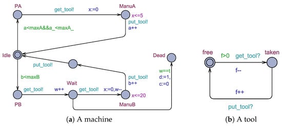
Figure 6. A network of timed automata modeling a reconfigurable job shop.

1.

The initial configuration $A_0$ of machines and a model of tools are depicted in Figure 6a,b, respectively;

2.

The synchronization channels get_tool and put_tool are present;

3.

Local clock x is used;

4.

Constant t represents the number of tools;

5.

Constants maxA, maxB and maxA_ correspond to the maximum number of products A, B, and $A^{\prime }$ to be manufactured, respectively;

6.

Local variables a, b, and a_ and global variables f and w are used to store the number of manufactured products A, B, and $A^{\prime }$, available tools, and waiting machines for a second tool, respectively;

7.

We distinguish a variable d used to indicate the presence of a deadlock;

8.

The use of local variable c is explained later.

When the value of w equals t, i.e., the number of waiting machines for a second tool equals the number of tools, the job shop is in a deadlock state. In this scenario, any waiting machine can identify the presence of a deadlock. This is modeled by an edge from location Waiting to location Dead (see Figure 6a) with the guard “w==t” and the effect “d:=1,c:=0”. Recall that variable d is used to indicate the presence of a deadlock state.

Once the value of d becomes one, the job shop must be reconfigured into the recovery mode. First, we apply reconfiguration $r_0$ illustrated in Figure 7 to the machine which detected the presence of a deadlock, such that its precondition is $g_{r_0}=(\mathtt{Dead},\mathtt{true},\mathtt{true})$. The obtained configuration is shown in Figure 8a.

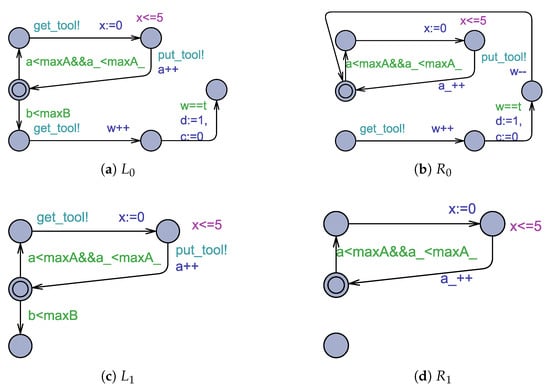
Figure 7. Transformation rules $r_0$ and $r_1$.

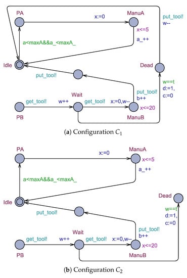
Figure 8. Configurations $C_1$ and $C_2$.

Remark 1.

Since the left- and right-hand sides and the interface of any rule have the same location set, we omit the interfaces of the rules in the figures presented in this section.

For the rest of the machines, we apply reconfiguration rule $r_1$ depicted in Figure 7 to each idle machine, whose precondition is $g_{r_1}=(\mathtt{Idle},\mathtt{true},\mathtt{d}==\mathtt{1})$. The obtained configuration is presented in Figure 8a.

Note that when $r_0$ is applied to a machine, it can move from location Dead to location Idle (see Figure 8a), and then release the tool. Then, any waiting machine can use that tool to resume the production of product B. After finishing, reconfiguration rule $r_1$ is applied to it.

When all tools are available, i.e., f==t, the job shop can return to its initial configuration by applying rules $r_2$ and $r_3$ shown in Figure 9. Rule $r_2$ is applicable to configuration $C_1$ whose pre- and postconditions are $g_{r_2}=(\mathtt{Idle},\mathtt{true},\mathtt{f}==\mathtt{t}||\mathtt{d}==\mathtt{0})$ and $u_{r_3}=(\varnothing ,“\mathtt{d}:=\mathtt{0},\mathtt{c}:=\mathtt{0}”)$, respectively. However, rule $r_3$ applies to configuration $C_2$ whose pre- and postconditions are $g_{r_3}=(\mathtt{Idle},\mathtt{true},(\mathtt{f}==\mathtt{t}\left|\right|\mathtt{d}==\mathtt{0})\&\&\mathtt{c}!=\mathtt{0})$ and $u_{r_3}=(\varnothing ,\mathtt{d}:=\mathtt{0})$. Here, variable c is used to prevent the application of $r_3$ to a machine that has detected the presence of deadlock before applying $r_2$. This is to ensure that $r_2$ only applies if $r_3$ has not been applied first.

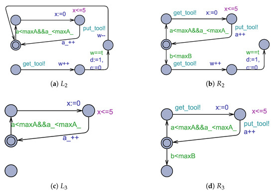
Figure 9. Transformation rules $r_2$ and $r_3$.

Now, we apply the unfolding algorithm to DTA $\mathcal{D}=⟨A_0,\{r_0,r_1,r_2,r_3\}⟩$, where initial configuration $A_0$ is shown in Figure 6a. The obtained TA $\mathcal{A}$ illustrated in Figure 10 is semantically equivalent to $\mathcal{D}$.

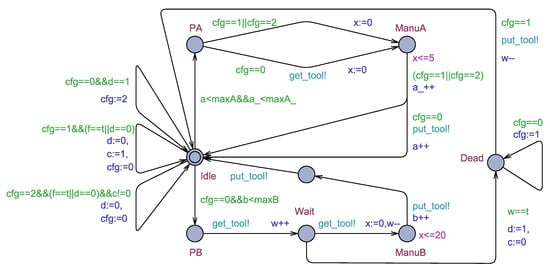
Figure 10. TA $\mathcal{A}$ semantic-equivalent to $\mathcal{D}$.

Finally, to verify some properties of the job shop, we use UPPAAL (i) to create an NTA consisting of three machines m${}_1$, m${}_2$, and m${}_3$ and two tools t${}_1$ and t${}_2$; (ii) and then to check certain properties. The obtained results are demonstrated in Table 1.

Table 1. Verification of some properties of interest.

Property	Meaning
A<> m1.cfg==0 && m2.cfg==0 && m3.cfg==0	The job shop can always return to its initial mode
A<> m1.Idle && m2.Idle && m3.Idle	The job shop can always return to its initial state
E<> m1.cfg!=0 && m2.cfg!=0 && m3.cfg!=0	A state in which m${}_1$, m${}_2$, and m${}_3$ are either in $C_1$ or $C_2$ is reachable
m1.Dead –> m1.cfg!=0	Whenever m${}_1$ reaches location Dead, then it can always change its configuration
A[] not (m1.cfg==2 && m2.cfg==2 && m3.cfg==2)	A state in which all machines are in $C_2$ at once is never reachable
E<> m1.cfg==1 && m2.cfg==1 && m3.cfg==1	A state in which all machines are in $C_1$ at once is reachable
A[] m1.a<=maxA && m1.b<=maxB && m1.a_<=maxA_	m${}_1$ never exceeds the production limit
t1.taken –> t1.free	A tool currently used by a machine will always be free after a while

Remark 2.

To ensure that a TA does not remain in a location indefinitely during model-checking, locationsPA,PB,Wait, andDeadare set as urgent. This means that an automaton must move immediately from these locations whenever possible. In fact, urgent locations can be expressed using only clocks. Hence, no modifications are needed to the proposed formalism level to support this feature.

8. Conclusions

Modern systems are designed with reconfigurable structures and a high flexibility to meet various complex requirements while maintaining cost-effectiveness. This creates a challenging issue in developing such systems and requires the use of rigorous tools such as timed automata.

The integration of graph transformation systems into formal methods brings several benefits. Nevertheless, several properties that need to be verified by designers become undecidable. To the best of our knowledge, there is no existing work that empowers timed automata by graph transformation systems to model dynamic structures.

In this paper, we presented an approach involving the transformation of timed automata. We leveraged the theory of the double-pushout approach to formulate the transformation rules, resulting in a new formalism called dynamic TA (DTA). Furthermore, we proposed an algorithm that transformed DTA into semantic-equivalent TA. This aimed to enable the use of existing TA analysis tools for the DTA analysis.

In future work, we will exploit the nature of the underlying models to ensure the preservation of global properties of TA models. This will allow a reduction of the temporal and spatial complexities of the verification process. Additionally, we will consider the relationship between rules, such as a critical pair analysis and compositional rule application, to provide more assistance to designers at the modeling step.

References

- Dima, A.; Bugheanu, A.M.; Boghian, R.; Madsen, D.O. Mapping Knowledge Area Analysis in E-Learning Systems Based on Cloud Computing. Electronics 2023, 12, 62. [Google Scholar] [CrossRef]
- Souri, A.; Rahmani, A.M.; Navimipour, N.J.; Rezaei, R. A hybrid formal verification approach for QoS-aware multi-cloud service composition. Clust. Comput. 2020, 23, 2453–2470. [Google Scholar] [CrossRef]
- Jasim, A.M.; Jasim, B.H.; Neagu, B.C.; Alhasnawi, B.N. Efficient Optimization Algorithm-Based Demand-Side Management Program for Smart Grid Residential Load. Axioms 2023, 12, 33. [Google Scholar] [CrossRef]
- Ecer, F.; Böyükaslan, A.; Hashemkhani Zolfani, S. Evaluation of Cryptocurrencies for Investment Decisions in the Era of Industry 4.0: A Borda Count-Based Intuitionistic Fuzzy Set Extensions EDAS-MAIRCA-MARCOS Multi-Criteria Methodology. Axioms 2022, 11, 404. [Google Scholar] [CrossRef]
- Souri, A.; Ghobaei-Arani, M. Cloud manufacturing service composition in IoT applications: A formal verification-based approach. Multimed. Tools Appl. 2022, 81, 26759–26778. [Google Scholar] [CrossRef]
- Awan, K.A.; Ud Din, I.; Almogren, A.; Khattak, H.A.; Rodrigues, J.J.P.C. EdgeTrust: A Lightweight Data-Centric Trust Management Approach for IoT-Based Healthcare 4.0. Electronics 2023, 12, 140. [Google Scholar] [CrossRef]
- El Ballouli, R.; Bensalem, S.; Bozga, M.; Sifakis, J. Programming dynamic reconfigurable systems. Int. J. Softw. Tools Technol. Transf. 2021, 23, 701–719. [Google Scholar] [CrossRef]
- Alur, R.; Dill, D. Automata for modeling real-time systems. In Automata, Languages and Programming, Proceedings of the 17th International Colloquium, Warwick University, UK, 16–20 July 1990; Paterson, M.S., Ed.; Springer: Berlin/Heidelberg, Germany, 1990; pp. 322–335. [Google Scholar]
- Souri, A.; Rahmani, A.M.; Jafari Navimipour, N. Formal verification approaches in the web service composition: A comprehensive analysis of the current challenges for future research. Int. J. Commun. Syst. 2018, 31, e3808. [Google Scholar] [CrossRef]
- Vaandrager, F. A First Introduction to UPPAAL. In Industrial Handbook; 2011; pp. 18–48. Available online: https://www.researchgate.net/publication/228919420_A_First_Introduction_to_Uppaal (accessed on 30 December 2022).
- Behrmann, G.; David, A.; Larsen, K.G. A tutorial on UPPAAL. In Proceedings of the Formal Methods for the Design of Real-Time Systems, Bertinoro, Italy, 13–18 September 2004; Springer: Berlin/Heidelberg, Germany, 2004; pp. 200–236. [Google Scholar]
- Chan, C.C.; Yang, C.Z.; Fan, C.F. Security Verification for Cyber-Physical Systems Using Model Checking. IEEE Access 2021, 9, 75169–75186. [Google Scholar] [CrossRef]
- Valero, V.; Díaz, G.; Cambronero, M.E. Timed Automata Modeling and Verification for Publish-Subscribe Structures Using Distributed Resources. IEEE Trans. Softw. Eng. 2017, 43, 76–99. [Google Scholar] [CrossRef]
- Lin, Q.Q.; Wang, S.L.; Zhan, B.H.; Gu, B. Modelling and verification of real-time publish and subscribe protocol using UPPAAL and Simulink/Stateflow. J. Comput. Sci. Technol. 2020, 35, 1324–1342. [Google Scholar] [CrossRef]
- Moussa, B.; Kassouf, M.; Hadjidj, R.; Debbabi, M.; Assi, C. An Extension to the Precision Time Protocol (PTP) to Enable the Detection of Cyber Attacks. IEEE Trans. Ind. Inform. 2020, 16, 18–27. [Google Scholar] [CrossRef]
- Mouelhi, S.; Laarouchi, M.E.; Cancila, D.; Chaouchi, H. Predictive Formal Analysis of Resilience in Cyber-Physical Systems. IEEE Access 2019, 7, 33741–33758. [Google Scholar] [CrossRef]
- Murata, T. Petri nets: Properties, analysis and applications. Proc. IEEE 1989, 77, 541–580. [Google Scholar] [CrossRef]
- Kulcsár, G.; Lochau, M.; Schürr, A. Graph-rewriting Petri nets. In Proceedings of the International Conference on Graph Transformation (ICGT 2018), Toulouse, France, 25–26 June 2018; Springer: Berlin/Heidelberg, Germany, 2018; pp. 79–96. [Google Scholar]
- Tigane, S.; Kahloul, L.; Benharzallah, S.; Baarir, S.; Bourekkache, S. Reconfigurable GSPNs: A modeling formalism of evolvable discrete-event systems. Sci. Comput. Program. 2019, 183, 102302. [Google Scholar] [CrossRef]
- Wang, H.; Wu, J.; Zhu, X.; Chen, Y.; Zhang, C. Time-Variant Graph Classification. IEEE Trans. Syst. Man Cybern. Syst. 2020, 50, 2883–2896. [Google Scholar] [CrossRef]
- Tigane, S.; Kahloul, L.; Hamani, N.; Khalgui, M.; Ali, M.A. On Quantitative Properties Preservation in Reconfigurable Generalized Stochastic Petri Nets. IEEE Trans. Syst. Man Cybern. Syst. 2022. early access. [Google Scholar] [CrossRef]
- Heckel, R.; Küster, J.M.; Taentzer, G. Confluence of Typed Attributed Graph Transformation Systems. In Proceedings of the Graph Transformation; Springer: Berlin/Heidelberg, Germany, 2002; pp. 161–176. [Google Scholar]
- Jayaraman, P.; Whittle, J.; Elkhodary, A.M.; Gomaa, H. Model Composition in Product Lines and Feature Interaction Detection Using Critical Pair Analysis. In Proceedings of the Model Driven Engineering Languages and Systems, Nashville, TN, USA, 30 September–5 October 2007; Springer: Berlin/Heidelberg, Germany, 2007; pp. 151–165. [Google Scholar]
- Taentzer, G. AGG: A Graph Transformation Environment for Modeling and Validation of Software. In Proceedings of the Applications of Graph Transformations with Industrial Relevance, Charlottesville, VA, USA, 27 September–1 October 2003; Springer: Berlin/Heidelberg, Germany, 2004; pp. 446–453. [Google Scholar]
- Göttmann, H.; Luthmann, L.; Lochau, M.; Schürr, A. Real-Time-Aware Reconfiguration Decisions for Dynamic Software Product Lines. In Proceedings of the 24th ACM Conference on Systems and Software Product Line, Montreal, QC, Canada, 19–23 October 2020; Association for Computing Machinery: New York, NY, USA, 2020. [Google Scholar] [CrossRef]
- Göttmann, H.; Bacher, I.; Gottwald, N.; Lochau, M. Static Analysis Techniques for Efficient Consistency Checking of Real-Time-Aware DSPL Specifications. In Proceedings of the 15th International Working Conference on Variability Modelling of Software-Intensive Systems (VaMoS ’21), Krems, Austria, 9–11 February 2021; Association for Computing Machinery: New York, NY, USA, 2021. [Google Scholar] [CrossRef]
- Zhou, W.; Liu, L.; Lü, S.; Zhang, P. Toward Formal Modeling and Verification of Resource Provisioning as a Service in Cloud. IEEE Access 2019, 7, 26721–26730. [Google Scholar] [CrossRef]
- Aman, B.; Ciobanu, G. Dynamics of reputation in mobile agents systems and weighted timed automata. Inf. Comput. 2022, 282, 104653. [Google Scholar] [CrossRef]
- Alur, R.; Henzinger, T.A.; Vardi, M.Y. Parametric real-time reasoning. In Proceedings of the Twenty-Fifth Annual ACM Symposium on Theory of Computing, San Diego, CA, USA, 16–18 May 1993; pp. 592–601. [Google Scholar]
- Bundala, D.; Ouaknine, J. Advances in Parametric Real-Time Reasoning. In Proceedings of the Mathematical Foundations of Computer Science 2014, Budapest, Hungary, 26–29 August 2014; Springer: Berlin/Heidelberg, Germany, 2014; pp. 123–134. [Google Scholar]
- Cordy, M.; Schobbens, P.Y.; Heymans, P.; Legay, A. Behavioural Modelling and Verification of Real-Time Software Product Lines. In Proceedings of the 16th International Software Product Line Conference, Beijing, China, 16–23 September 2016; Association for Computing Machinery: New York, NY, USA, 2012; Volume 1, pp. 66–75. [Google Scholar] [CrossRef]
- Luthmann, L.; Stephan, A.; Bürdek, J.; Lochau, M. Modeling and Testing Product Lines with Unbounded Parametric Real-Time Constraints. In Proceedings of the 21st International Systems and Software Product Line Conference (SPLC ’17), Sevilla, Spain, 25–29 September 2017; Association for Computing Machinery: New York, NY, USA, 2017; Volume A, pp. 104–113. [Google Scholar] [CrossRef]
- Luthmann, L.; Gerecht, T.; Stephan, A.; Bürdek, J.; Lochau, M. Minimum/maximum delay testing of product lines with unbounded parametric real-time constraints. J. Syst. Softw. 2019, 149, 535–553. [Google Scholar] [CrossRef]
- Bürdek, J.; Lochau, M.; Bauregger, S.; Holzer, A.; von Rhein, A.; Apel, S.; Beyer, D. Facilitating Reuse in Multi-goal Test-Suite Generation for Software Product Lines. In Proceedings of the Fundamental Approaches to Software Engineering, London, UK, 11–18 April 2015; Springer: Berlin/Heidelberg, Germany, 2015; pp. 84–99. [Google Scholar]
- Latreche, F.; Belala, F. RDTA: Recursive and Dynamic Timed Automata for Web Services Composition Analysis. Int. J. Embed.-Real-Time Commun. Syst. (IJERTCS) 2014, 5, 42–67. [Google Scholar] [CrossRef]
- Campana, S.; Spalazzi, L.; Spegni, F. Dynamic Networks of Timed Automata for collaborative systems: A network monitoring case study. In Proceedings of the 2010 International Symposium on Collaborative Technologies and Systems, Chicago, IL, USA, 17–21 May 2010; pp. 113–122. [Google Scholar] [CrossRef]
- Attie, P.C.; Lynch, N.A. Dynamic input/output automata: A formal and compositional model for dynamic systems. Inf. Comput. 2016, 249, 28–75. [Google Scholar] [CrossRef]
- Bettira, R.; Kahloul, L.; Khalgui, M.; Li, Z. Reconfigurable Hierarchical Timed Automata: Modeling and Stochastic Verification. In Proceedings of the 2019 IEEE International Conference on Systems, Man and Cybernetics (SMC), Bari, Italy, 6–9 October 2019; pp. 2364–2371. [Google Scholar]
- Bettira, R.; Kahloul, L.; Khalgui, M. A Novel Approach for Repairing Reconfigurable Hierarchical Timed Automata. In Proceedings of the 15th International Conference on Evaluation of Novel Approaches to Software Engineering (ENASE 2020), Online, 5–6 May 2020; pp. 398–406. [Google Scholar]
- Tigane, S.; Kahloul, L.; Baarir, S.; Bourekkache, S. Dynamic GSPNs: Formal Definition, Transformation towards GSPNs and Formal Verification. In Proceedings of the 13th EAI International Conference on Performance Evaluation Methodologies and Tools (VALUETOOLS ’20), Tsukuba, Japan, 18–20 May 2020; Association for Computing Machinery: New York, NY, USA, 2020; pp. 164–171. [Google Scholar]
Disclaimer/Publisher’s Note: The statements, opinions and data contained in all publications are solely those of the individual author(s) and contributor(s) and not of MDPI and/or the editor(s). MDPI and/or the editor(s) disclaim responsibility for any injury to people or property resulting from any ideas, methods, instructions or products referred to in the content. |
© 2023 by the authors. Licensee MDPI, Basel, Switzerland. This article is an open access article distributed under the terms and conditions of the Creative Commons Attribution (CC BY) license (https://creativecommons.org/licenses/by/4.0/).