The Kinetic Theory of Mutation Rates

Abstract

The Luria–Delbrück mutation model is a cornerstone of evolution theory and has been mathematically formulated in a number of ways. In this paper, we illustrate how this model of mutation rates can be derived by means of classical statistical mechanics tools—in particular, by modeling the phenomenon resorting to methodologies borrowed from classical kinetic theory of rarefied gases. The aim is to construct a linear kinetic model that can reproduce the Luria–Delbrück distribution starting from the elementary interactions that qualitatively and quantitatively describe the variations in mutated cells. The kinetic description is easily adaptable to different situations and makes it possible to clearly identify the differences between the elementary variations, leading to the Luria–Delbrück, Lea–Coulson, and Kendall formulations, respectively. The kinetic approach additionally emphasizes basic principles which not only help to unify existing results but also allow for useful extensions.

1. Introduction

Statistical physics represents a powerful approach to the mathematical modelling of living systems composed of large numbers of growing organisms interacting with each other and/or the environment, and permits one to understand the relationships between the parameters defining the microscopic rules and the resulting macroscopic statistical results. For this reason, the last two decades have seen a trend towards applying tools from statistical mechanics to interdisciplinary fields ranging from the classical biological context to new aspects of socio-economic phenomena [1,2,3,4].

In order to best justify the statistical physics approach classically used for gas dynamics where the number of molecules in a mole is characterized by Avogadro’s constant [5], the system under consideration must satisfy some minimum requirements. On the one hand, the population composing the system must be very large (of the order of millions), and on the other hand, the time in which we observe the system must be long enough to ensure that we are close to a stable statistical profile.

An issue that naturally satisfies these requirements is the time evaluation of the number of mutation rates, a challenging problem which has attracted the interest of generations of both geneticists and mathematicians. This problem, which is essentially a matter of evaluating the growth of a population, originated from a series of classical experiments conducted by Luria and Delbrück [6], which led to a fundamental example of how mathematics can be used to estimate mutation rates. The model proposed by Luria and Delbrück assumed deterministic growth of mutant cells, which seemed too stringent an assumption to allow for efficient extraction of reliable information about mutation rates from experimental data.

This shortcoming of Luria and Delbrück’s model was overcome a few years later by a slightly different mathematical formulation proposed by Lea and Coulson [7], who adopted Yule’s stochastic birth process to simulate the growth of mutant cells. In the decades that followed, the Lea–Coulson formulation gained such a prominent place in the study of mutation rates that this formulation is now commonly referred to as the Luria–Delbrück model, as documented by the long list of research articles dedicated to the subject (see [8,9,10,11,12,13,14,15,16,17] and numerous others cited in Zheng’s seminal article [18]). In his seminal article, Zheng examines the various mathematical formulations, focusing on important practical issues closely related to the distribution of the number of mutants. It is evident that almost all these formulations are predominantly based on probabilistic arguments.

Adopting the point of view of statistical physics, the Luria–Delbrück problem was first modeled only a few years ago by Kashdan and one of the authors in [19]. In that work, a kinetic description of the density of mutation rates was considered, in which the Luria–Delbrück distribution appears as a suitable limit of a linear kinetic equation describing the growth of mutated cells. Following the original model by Luria and Delbrück’s, mutation is, in the kinetic context, a consequence of a specific elementary update rule, where both normal and mutant cells grow deterministically but mutations occur randomly. The analysis in [19] was later extended by one of the present authors in [20] to cover Lea and Coulson’s model [7], which is based on a different formulation, according to which normal cells grow deterministically but mutants grow stochastically [21].

As discussed in [22], the kinetic equations introduced in [19,20] (see also [4]) are well-posed from a mathematical point of view, and various properties of the unique solutions are available to be studied from a numerical point of view. The pioneering work [19] has been credited for outlining the power of kinetic methodology to model growth processes in the field of mutation rates.

Indeed, for years, various concepts and techniques of statistical physics have been successfully applied to a wide variety of complex systems, physical and otherwise, in an attempt to understand, starting from the elementary interactions, the emergent properties that appear therein.

In particular, this methodology has been employed to write down realistic evolution models for wealth in economics [23,24,25,26,27,28,29,30,31,32,33]. In this context, it was rigorously shown that the asymptotic profile of wealth distribution and the possibility to have Pareto-type tails depend completely on the microscopic structure of binary trades [30,34].

In the kinetic description of mutation rates, the core of the methodology is to identify the linear elementary interaction rule, which drives the underlying process of mutation, in order to write a kinetic equation of the Boltzmann type for the distribution density of the mutated cells. As is common in this approach, the construction of the kinetic equation emphasizes the differences between the microscopic interaction rules of the original Luria–Delbrück distribution and the Lea–Coulson modification. Similarly to the collisional Boltzmann equation of rarefied gases in the case of Maxwell-type interactions [5], the kinetic description allows one to use in a natural and powerful way the weak formulation in terms of the Fourier transform [35], which clarifies the nature of the assumption made by Lea and Coulson [7], namely, the choice of a Yule process for the random growth of mutated cells [21].

This challenging application shows that the kinetic description based on linear interactions is powerful and flexible, and allows us in most cases to establish a direct connection between the elementary interaction and the consequent macroscopic behavior. Once again, as happens in the study of wealth distribution in a multi-agent society, where the characteristics of the binary trade are reflected in the steady profile of wealth, or in opinion formation [36], where the details of the binary exchange of opinion produce the steady distribution profile of opinion in the system, one can learn from microscopic dynamics the forthcoming macroscopic behavior of mutant cells, and associate with the various models the corresponding elementary mechanism of interaction.

Moreover, the kinetic description in terms of elementary interactions indicates in most cases a way to design numerical algorithms based on Monte Carlo methods useful to following the process under study, where the numerical solution satisfies the main physical properties of the continuous one [4,37,38]. Consequently, it provides a new way to approach the numerical simulation problem of mutation rates and to compare it with existing ones [39,40].

2. Basics of Kinetic Theory

The objective of linear kinetic theory is to determine the time evolution of the statistical distribution of a phenomenon subject to frequent elementary variations of the same type. Let $x\in I\subseteq \mathbb{R}$ denote the amount of a certain evolving quantity (wealth, opinion, weight, etc.), and let us denote by $f(x,t)dx$, $x\in \mathbb{R}$, the amount of this quantity which at time $t\ge 0$ lies in the interval $(x,x+dx)$. Suppose also that the quantity $f(x,t)$ changes over time due to repeated linear elementary variations given by

$$x_{*}=Ax+B,$$

(1)

where the coefficients A and B can be constant, or more generally, random quantities. According to classical kinetic theory, the two terms characterizing variation (1) refer to an internal variation (measured by A) and an external variation (measured by B). The latter variation can be understood as a consequence of the presence of the external environment, usually referred to as the background.

The evolution in time of the density $f(x,t)$ is captured by looking at its variations in the observable quantities $\phi \left(x\right)$ over time  [4,5], given by the equation

$$\frac{d}{dt}{\int }_{\mathbb{R}}\phi \left(x\right)f(x,t)dx=\frac{1}{\tau }〈{\int }_{\mathbb{R}}\left[\phi \left(x_{*}\right)-\phi \left(x\right)\right]f(x,t)dx〉.$$

(2)

The integral on the right-hand side of Equation (2) measures the variation in the observable quantity $\phi$ consequent to the variation of the quantity x under consideration, determined by the elementary law (1). The presence of the mean $\langle ·\rangle$ is due to the (possible) presence of random quantities in the coefficients A and B. The positive part of the integral quantifies the variation in $\phi$ consequent to the change from $x_{*}$ to x (gain term), and the negative part of the integral quantifies the variation in $\phi$ consequent to the change from x to $x_{*}$ (loss term). Last, the time frequency $1/\tau$ is a measure of the speed at which the phenomenon relaxes towards the steady or self-similar solution [5]. This quantity can be easily absorbed by a suitable scaling of the time variable.

Note that, starting from Equation (2), it is crucial to determine the evolution of the principal moments of the distribution function $f(x,t)$, which is obtained by choosing the observable quantity $\phi \left(x\right)=x^n$, $0\le n\in \mathbb{N}$, and consequently to identify eventual conservation laws.

As recently described in [41], this methodology can be profitably applied both to describe the well-known Galton’s experiment  [42,43] (cf. also Stigler [44]) and to obtain information about its behavior over long periods of time. Indeed, the Galton board, also known as the Galton box or quincunx or bean machine, represents a clear visual approach to link repeated elementary interactions to a consequent universal steady state density. In this famous experiment, balls subject to gravity exhibit repeated symmetric variations of direction before falling on the ground. Each variation is determined by interaction of the ball with a pin. Pins are equi-spaced on equally spaced horizontal rows, so that each pin on the n-th row forms with the two nearest pins on n+1-th row an isosceles triangle. At the bottom, if the number of balls is sufficiently high, one can catch a glimpse of the profile of the Gaussian density

$$M\left(x\right)=\frac{1}{\sqrt{2\pi {\sigma }^2}}exp\left\{-\frac{x^2}{2{\sigma }^2}\right\}.$$

Galton’s experiment corresponds to a sequence of Bernoulli trials (or binomial trials), where the trial is a random experiment with exactly two possible outcomes, success and failure. The probability of success ($1/2$ in Galton’s experiment) is the same each time the experiment is conducted. The classical way to give a mathematical explanation of the result is to switch from the discrete to the continuous description. In the half-plane $(x,t)$, $t\ge 0$, the continuous representation of the variation over time in the probability $p(x,t)dx$ of finding the ball in the interval $(x,x+\Delta x)$ at time $t+\Delta t\ge 0$, is given by the relation

$$p(x,t+\Delta t)=\frac{1}{2}p(x+\Delta x,t)+\frac{1}{2}p(x-\Delta x,t).$$

Expanding in Taylor’s series, at the first order in time, the left-hand side, and at the second order in position, the right-hand side, shows that in the limit ${(\Delta x)}^2/\Delta t\to {\sigma }^2>0$, $p(x,t)$ satisfies the linear diffusion equation:

$$\frac{\partial p}{\partial t}=\frac{{\sigma }^2}{2}\frac{{\partial }^{2}p}{\partial x^2}.$$

Now, it is sufficient to observe that in Galton’s experiment, the repeated trials start from the value $x=0$. Consequently, if the number of repeated trials is large enough, and the discrete solution is close to the continuous one, the resulting profile is well approximated by the source-type solution of the linear diffusion equation. The source-type solution to the diffusion equation at time $t>0$ is the Gaussian density:

$$M(x,t)=\frac{1}{\sqrt{2\pi {\sigma }^{2}t}}exp\left\{-\frac{x^2}{2{\sigma }^{2}t}\right\}.$$

This gives an answer to the visual result of the experiment.

We now resort to the classical approach of the collisional kinetic theory described above [41]. We consider a very large number of identical Galton bean machines and show a proof of the experiment simultaneously on all machines. We denote by $f(x,t)dx$, $x\in \mathbb{R}$ the amount of balls that at time $t\ge 0$ lie in the interval $(x,x+dx)$. The function $f(x,t)$ changes over time as the balls are subject to interactions that change their positions. The elementary interaction of type (1) is now given by

$$x_{*}=x+\sigma \eta ,$$

(3)

where $\eta$ is a symmetric random variable taking values $\pm 1$ with probability $1/2$ ( $2\sigma >0$ is the constant distance between pins). According to collisional kinetic theory, the random variation in (3) is a consequence of the presence of the external environment, usually referred to as the background. Let us further suppose that the trial starts with balls located in $x=0$, and let us compute, via the kinetic Equation (2), the time evolution of the principal moments.

The choice $\phi \left(x\right)=1$ gives

$$\frac{d}{dt}{\int }_{\mathbb{R}}f(x,t)dx=0,$$

which shows that the mass is preserved in time. This means that $f(x,t)$ remains a probability density for all $t\ge 0$, if it is so initially.

Analogously, if we choose $\phi \left(x\right)=x$, since $\langle x_{*}-x\rangle =\langle \eta \rangle =0$, we find that the mean value is preserved in time. Thus, the mean value of $f(x,t)$, equal to zero at time $t=0$, is equal to zero for all times $t\ge 0$.

Moreover, since $\langle x_{*}^2-x^2\rangle =\langle 2x\sigma \eta +{\sigma }^2{\eta }^2\rangle ={\sigma }^2$,

$$\frac{d}{dt}{\int }_{\mathbb{R}}{x}^{2}f(x,t)dx=\frac{{\sigma }^2}{\tau }{\int }_{\mathbb{R}}f(x,t)dx=\frac{{\sigma }^2}{\tau }.$$

Consequently, the variance in the density function diverges with time. This shows that we cannot expect that the solution will tend for large times towards a steady state of finite variance.

This unpleasant feature can be eliminated by appropriately restricting the domain. Having fixed a positive constant $\lambda <1$, we introduce the modified interaction

$$x_{*}=x(1-\lambda )+\sigma \eta ,$$

(4)

which still belongs to the class of interactions (1).

This restriction does not modify the main features of the shape of $f(x,t)$. Indeed, the mean value of $f(x,t)$ remains equal to zero for all times $t\ge 0$. Since now $\langle x_{*}^2-x^2\rangle ={\sigma }^2-\lambda (2-\lambda )x^2$, we obtain

$$\frac{d}{dt}{\int }_{\mathbb{R}}{x}^{2}f(x,t)dx=\frac{{\sigma }^2}{\tau }{\int }_{\mathbb{R}}f(x,t)dx-\frac{\lambda (2-\lambda )}{\tau }{\int }_{\mathbb{R}}{x}^{2}f(x,t)dx,$$

(5)

which implies that the variance of the density function remains uniformly bounded in time. By solving the differential equation, Equation (5), we obtain

$${\int }_{\mathbb{R}}{x}^{2}f(x,t)dx=e^{-\lambda (2-\lambda )t/\tau }{\int }_{\mathbb{R}}{x}^2{f}_0\left(x\right)dx+\frac{{\sigma }^2}{\lambda (2-\lambda )}\left[1-e^{-\lambda (2-\lambda )t/\tau }\right].$$

This suggests that, in presence of the elementary variation (4), the solution to the kinetic equation could relax towards a universal steady state, namely, a distribution that depends on the initial state only through its moments, and that is fully characterized by the interaction (4). This feature can be captured by resorting to a second ingredient, which is now part of classical kinetic theory, which consists of studying the problem in the so-called grazing collision limit (cf. [4,45] and the references therein). By this limit procedure, we mainly consider only interactions which produce a very small modification of the pre-interaction value (from this comes the term grazing, which is borrowed from the kinetic theory of rarefied gases, where grazing interactions describe a binary collision in which the outgoing post-collision velocities remain very close to the ingoing ones), while waiting enough time to see finite variations in the observable quantities.

Let us apply the grazing procedure to the modified Galton’s experiment. This corresponds to reducing the size of the triangles, the shrinking parameter, and the time frequency in such a way as to still observe the evolution of the variance towards a value bounded away from zero. By looking at the coefficients of Equation (5), we can realize that this can be done by setting, for $\epsilon \ll 1$,

$${\sigma }^2\to \epsilon {\sigma }^2;\lambda \to \epsilon \lambda ;\tau \to \epsilon \tau .$$

(6)

The meaning of the scaling (6) is clear. Within this scaling, each interaction produces only a small variation in the position variable. To see its effect on the variation of the observable, one has to suitably increase the time frequency of the interactions!

In this regime, for a given regular observable function $\phi \left(x\right)$, by expanding it in a Taylor series up to the second order and neglecting terms of order $o\left(\epsilon \right)$ (cf. [45] for details), we can write

$$\langle \phi \left(x_{*}\right)-\phi \left(x\right)\rangle \simeq {\phi }^{\prime }\left(x\right)\langle x_{*}-x\rangle +\frac{1}{2}{\phi }^{″}\left(x\right)\langle {(x_{*}-x)}^2\rangle \simeq$$

$$\epsilon \left[-\lambda x{\phi }^{\prime }\left(x\right)+\frac{{\sigma }^2}{2}{\phi }^{″}\left(x\right)\right].$$

By setting for simplicity, $\tau =\epsilon$, we conclude that the kinetic equation is well approximated by

$$\frac{d}{dt}{\int }_{\mathbb{R}}\phi \left(x\right)f(x,t)dx={\int }_{\mathbb{R}}\left[-\lambda x{\phi }^{\prime }\left(x\right)+\frac{{\sigma }^2}{2}{\phi }^{″}\left(x\right)\right]f(x,t)dx.$$

(7)

Equation (7) is the weak form of the Fokker–Planck Equation [45]

$$\frac{\partial f(x,t)}{\partial t}=\frac{{\sigma }^2}{2}\frac{{\partial }^{2}f(x,t)}{\partial x^2}+\lambda \frac{\partial \left(xf\right(x,t\left)\right)}{\partial x}.$$

The equilibrium solution of the Fokker–Planck Equation (of unit mass) is the Gaussian probability density [45]:

$$f_{\infty }\left(x\right)=\sqrt{\frac{\lambda }{\pi {\sigma }^2}}exp\left\{-\frac{\lambda x^2}{{\sigma }^2}\right\}.$$

(8)

Therefore, the kinetic approach is consistent with the experimental evidence.

Remark 1.

The kinetic description remains valid even in the case in which the shrinking parameter λ is assumed to be equal to zero. In this case, instead of the Fokker–Planck equation, we obtain that the grazing limit produces the linear diffusion equation classically obtained by adopting the continuous description in the half-plane we briefly illustrated before.

Remark 2.

In contrast with the classical Galton bean machine, where, as explained above, the normal density can be observed only if all the repeated trials start from $x=0$, in the kinetic approach, which leads to the Fokker–Planck equation, any initial probability density of finite variance can be shown to converge towards the Gaussian density (8) [45].

3. The Kinetic Descriptions of Mutation Rates

The procedure of Section 2 is quite general and can be easily adapted for studying the problem of mutation rates. This will be the object of this Section. In detail, and in the words of a referee, we will show how the basic equations of three models of the Luria–Delbrück experiment can be derived. These models are: (i) Delbrück’s model in which the quantity of normal cells grows exponentially from a single cell. This simple dynamical system drives a Poisson process of mutation events and mutations in mutant clones which grow exponentially with the same rate, which may differ from the normal growth rate. Mutant clones grow independently of each other and of the background normal cell population. (ii) The Lea–Coulson variation in which mutant clones grow in an independent linear birth processes. (iii) The Bartlett model, according to which the whole process is described as a two-type branching process. Normal cells have an exponentially distributed lifetime, at the end of which they divide in two. There is a small probability that exactly one of the daughter cells mutates and initiates a mutant clone, which grows as in Model (ii).

The mutant population quantity (for (i)) or size (for (ii)) can be represented as a compound Poisson process (as in [11]), thereby allowing a simple derivation of the basic equations for the Laplace–Stieltjes transform or probability generating function, as appropriate. Model (iii) is handled by considering what happens at the first normal division in the time interval $(0,t]$, if there is one.

Before illustrating the kinetic approach, let us briefly discuss the classical setting. The first mathematical description of the mutation process, which was subsequently modified by Lea and Coulson, goes back to Luria and Delbrück [6]. As all subsequent formulations are simple variations of this formulation, we detail below its underlying assumptions.

The process starts at time $t=0$ with one normal cell and no mutants. Normal cells are assumed to grow deterministically at a constant rate ${\beta }_1$. Therefore, the number of normal cells at time $t>0$ is $N\left(t\right)=e^{{\beta }_{1}t}$.

Mutants grow deterministically at a constant rate ${\beta }_2$. If a mutant is generated by a normal cell at time $s>0$, then the clone spawned by this mutant will be of size $e^{{\beta }_2(t-s)}$ for any $t>s$. Mutations occur randomly at a rate proportional to $N\left(t\right)$. If $\mu$ denotes the per-cell, per-unit-time mutation rate, then the standard assumption is that mutations occur in accordance with a Poisson process having the intensity function

$$\nu \left(t\right)=\mu N\left(t\right)=\mu e^{{\beta }_{1}t}.$$

(9)

Consequently, the expected number of mutations occurring in the time interval $[0,t)$ is

$${\int }_0^t\nu \left(s\right)ds=\frac{\mu }{{\beta }_1}\left(e^{{\beta }_{1}t}-1\right).$$

Let $X\left(t\right)$ denote the number of mutants existing at time t and $f(n,t)$ the probability of having n mutants at time t. The previous assumptions imply that $X\left(t\right)$ can be expressed as

$$X\left(t\right)=\sum _{i=1}^{M\left(t\right)}exp\left\{{\beta }_2(t-{\tau }_i)\right\},\mathrm{if}M\left(t\right)\ge 1,$$

(10)

while

$$X\left(t\right)=0\mathrm{if}M\left(t\right)=0.$$

where ${\tau }_i$ represents the random times at which mutations occur, and $M\left(t\right)$ stands for the mutation process, which is a Poisson process with the intensity function $\nu \left(t\right)$ given in (9). The probabilistic description (10) allows for recovering the various quantities, such as mean, variance, and cumulants [46] (cf. also the detailed historical description in [18]).

An interesting alternative to the probabilistic construction described above is to use the approach of Section 2. Within this approach, the study of the time evolution of the probability distribution $f(n,t)$ of mutants, together with a reasonable explanation of the growth process induced by this distribution, is achieved by means of linear kinetic models [19,20].

In order to bring the study of distribution of mutants back to a kinetic description, we introduce a system of agents characterized by a trait $v\ge 0$ and denote by $f(v,t)$ the distribution in the population of trait v at time $t\ge 0$. We will assume for simplicity that the trait v is a continuous parameter, $v\in {\mathbb{R}}_{+}$, and that the time variation of the distribution $f(v,t)$ of the trait is based on elementary interactions of type (1). The interaction rule described by the previous probabilistic description indeed corresponds to assuming that, at time $t>0$, the microscopic growth of the trait under investigation is driven by the elementary law of variation

$$v^{*}=(1+{\beta }_2)v+\eta \left(t\right),$$

(11)

where $\eta \ge 0$, describing the interaction of agents with the background, is a discrete random variable distributed according to a Poisson density $p\left(\nu \right(t\left)\right)$ of intensity given by (9).

This makes an essential difference between the elementary interactions considered in Section 2 and the present one. Now, the intensity of the elementary interaction varies in time, due to time variable random contribution. For that reason, the principal moments of the distribution, including the mean value, are time-dependent.

Additionally, for any given v, the value of the trait after the interaction can only assume the values

$$v_i^{*}=(1+{\beta }_2)v+i,i\in \mathbb{N}.$$

The interaction (11) then leads to the kinetic Equation (in weak form) [19]

$$\frac{d}{dt}{\int }_{{\mathbb{R}}_{+}}f(v,t)\phi \left(v\right)dv=\sum _{i=1}^{\infty }{p}_i\left(\nu \left(t\right)\right){\int }_{{\mathbb{R}}_{+}}\left(\phi \left(v_i^{*}\right)-\phi \left(v\right)\right)f(v,t)dv,$$

(12)

where $\phi \left(v\right)$ is a smooth function.

Remark 3.

Equation (12) describes the time evolution of the distribution of the trait v in a system of agents in terms of a kinetic equation, in which the right-hand side quantifies the variation of the trait consequent to the elementary upgrade (11), as it results from the internal growth and the external growth due to the presence of the background. However, the abstract evolution of the solution of the kinetic Equation (12) can be used to describe the evolution of the number of mutants, in case this evolution is determined by an upgrade of type (11). For this reason, and without problems of misunderstanding, we will use with the same meaning the terms interaction and mutation.

Going back to the mutation problem, the condition of having no mutants at time $t=0$ translates into the initial condition

$$f(v,t=0)=f_0\left(v\right)={\delta }_0\left(v\right),$$

(13)

where ${\delta }_a\left(v\right)$ indicates as usual the Dirac delta function concentrated at $v=a$.

Interaction (11) belongs to the class of linear interactions (1), and it is sufficiently flexible to describe both the original Luria–Delbrück formulation and the Lea–Coulson formulation.

It is imperative to verify whether in any of the aforementioned formulations of the growth of the mutant cells, the microscopic process is due to two simultaneous events. The first one describes the intrinsic growth of the mutants, which can be represented by a general interaction of type

$$v^{\prime }=v+\mathcal{L}\left(v\right),$$

(14)

where $v\to \mathcal{L}\left(v\right)\ge 0$, as in (1), is a linear map acting on v. Note that the choice $\mathcal{L}\left(v\right)={\beta }_{2}v$ gives the classical Luria–Delbrück relation (11). The map can be either deterministic or random. In the latter case, corresponding to the Lea–Coulson formulation, when denoting by $\langle ·\rangle$ the mathematical expectation, in order to maintain the same mean growth of the deterministic interaction, we will assume that

$$\langle \mathcal{L}\left(v\right)\rangle ={\beta }_{2}v.$$

(15)

The second event describes the growth of the mutant cells due to the presence of the normal ones which produce new mutants at the jump times of the Poisson process $M\left(t\right)$ as in (10) above. As described before, this corresponds to assuming that the mutants are immersed in a background (of normal cells), which, due to its random mutation rule, facilitates interactions which increase the number of mutants according to the time-dependent probability density $M(w,t)$. In the Luria–Delbrück setting, the probability density of the background depends on time, and it is a probability mass function of Poisson type, with intensity $\nu \left(t\right)=\mu N\left(t\right)$.

This means to say that the background density takes the form

$$M(w,t)=\sum _{k\ge 0}\frac{\nu {\left(t\right)}^k{e}^{-\nu \left(t\right)}}{k!}{\delta }_k\left(w\right),$$

where, as in (13), ${\delta }_k\left(w\right)$ indicate the Dirac delta functions located in the points $k\in {\mathbb{N}}_{+}$. Consequently,

$${\int }_{{\mathbb{R}}_{+}}M(w,t)dw=1;{\int }_{{\mathbb{R}}_{+}}wM(w,t)dw=\mu e^{{\beta }_{1}t}.$$

(16)

Coupling the interaction (11) with the contribution due to the background, one obtains the general elementary interaction [20]

$$v^{*}=v+\mathcal{L}\left(v\right)+w.$$

(17)

Following the arguments of Section 2, the effect of interactions (17) on the time variation of the mutant density can be quantitatively described by a linear Boltzmann-type equation in which the variation of the density $f=f(v,t)$ is due to a balance between gain and loss terms that, for the given value v, take into account all the interactions of type (17), which end up with the number v (gain term), and all the interactions which, starting from the number v, lose this value after interaction (loss term). For a given observable $\phi \left(v\right)$, the kinetic equation for the density $f(v,t)$ can be written in the form

$$\frac{d}{dt}{\int }_{{\mathbb{R}}_{+}}\phi \left(v\right)f(v,t)dv=〈{\int }_{{\mathbb{R}}_{+}^2}\left(\phi \left(v^{*}\right)-\phi \left(v\right)\right)f(v,t)M(w,t)dvdw〉.$$

(18)

In Equation (18), the presence of $\langle ·\rangle$ takes into account the possibility that $\mathcal{L}\left(v\right)$ could be a random quantity. Note that the choice $\phi \left(v\right)=1$ implies that $f(v,t)$ remains a probability density if it is so initially:

$${\int }_{{\mathbb{R}}_{+}}f(v,t)dv={\int }_{{\mathbb{R}}_{+}}{f}_0\left(v\right)dv=1.$$

(19)

Moreover, given the elementary interaction (17), choosing $\phi \left(v\right)=v$ shows that the total mean number of mutants satisfies the differential equation

$$\frac{dm\left(t\right)}{dt}={\int }_{{\mathbb{R}}_{+}}\langle \mathcal{L}\left(v\right)\rangle f(v,t)dv+\mu e^{{\beta }_{1}t}.$$

(20)

We note that the choice $\langle \mathcal{L}\left(v\right)\rangle ={\beta }_{2}v$ implies

$$\frac{dm\left(t\right)}{dt}={\beta }_{2}m\left(t\right)+\mu e^{{\beta }_{1}t},$$

(21)

which, coupled with the initial condition $m\left(0\right)=0$ induced by (13), leads to the explicit computation of the mean value of the Luria–Delbrück distribution (${\beta }_1\ne {\beta }_2$), for any time $t>0$:

$$m\left(t\right)=\frac{\mu }{{\beta }_1-{\beta }_2}\left(e^{{\beta }_{1}t}-e^{{\beta }_{2}t}\right).$$

This expression is independent of the particular form of the map $\mathcal{L}$, provided the map is such that condition (15) is satisfied. In other words, at the level of the growth of the mean value, the original formulation by Luria–Delbrück, and its modification considered by Lea–Coulson, produce the same time behavior.

The Role of the Fourier Transform

As is usually done for linear kinetic models of this type [4], most of the analytical properties of the solution can be obtained by resorting to Fourier analysis. However, since we are working with distribution functions depending on a nonnegative variable v, a similar analysis can be done by resorting to the Laplace–Stieltjes transform [47].

The choice $\phi \left(v\right)=e^{-i\xi v}$ in the Formulation (18) is, in fact, equivalent to the Fourier-transformed equation

$$\frac{\partial \widehat{f}(\xi ,t)}{\partial t}=\widehat{M}(\xi ,t){\int }_{{\mathbb{R}}_{+}}\langle e^{-i\xi \mathcal{L}\left(v\right)}\rangle e^{-i\xi v}f(v,t)dv-\widehat{f}(\xi ,t).$$

(22)

In (22), we used the fact that $M(w,t)$ is a probability mass function, so that $\widehat{M}(0,t)=1$. The initial condition (13) turns into

$${\widehat{f}}_0\left(\xi \right)=1.$$

Note that, since $M(w,t)$ is a probability mass function of Poisson type with intensity $\nu \left(t\right)=\mu e^{{\beta }_{1}t}$,

$$\widehat{M}(\xi ,t)=exp\left\{\mu e^{{\beta }_{1}t}\left(e^{-i\xi }-1\right)\right\}.$$

Clearly, the explicit evaluation of the gain term on the right-hand side of Equation (22) requires the knowledge of $\mathcal{L}\left(v\right)$. In the case in which $\mathcal{L}\left(v\right)={\beta }_{2}v$, Equation (22) takes the form [4,20]

$$\frac{\partial \widehat{f}(\xi ,t)}{\partial t}=\widehat{M}(\xi ,t)\widehat{f}\left((1+{\beta }_2)\xi \right)-\widehat{f}(\xi ,t).$$

(23)

Likewise, by assuming that $\mathcal{L}\left(v\right)$ is a Poisson variable of mean value ${\beta }_{2}v$, thereby satisfying (15),

$$\langle e^{-i\xi \mathcal{L}\left(v\right)}\rangle =exp\left\{{\beta }_{2}v\left(e^{-i\xi }-1\right)\right\}=exp\left\{-iv{\beta }_{2}i\left(e^{-i\xi }-1\right)\right\},$$

(24)

and Equation (22) becomes [20]

$$\frac{\partial \widehat{f}(\xi ,t)}{\partial t}=\widehat{M}(\xi ,t)\widehat{f}\left(\xi +{\beta }_{2}i\left(e^{-i\xi }-1\right),t\right)-\widehat{f}(\xi ,t).$$

(25)

Equations (23) and (25) differ only in the gain term on the right-hand side, where the Fourier transform of the probability density is evaluated at different points.

The existence of a solution to Equations (23) and (25) can be seen easily using well-consolidated techniques of common use in the kinetic theory of social phenomena [22,45]. The main argument is to resort to the class of Fourier-based metrics introduced in [48].

For a given pair of random variables X and Y distributed according to f and g these metrics read

$$d_r(X,Y)=\underset{\xi \in \mathbb{R}}{sup}\frac{|\widehat{f}\left(\xi \right)-\left(\xi \right)|}{{\left|\xi \right|}^r},r>0.$$

(26)

As shown in [48], the metric $d_r(X,Y)$ is finite any time the densities f and g have equal moments up to $\left[r\right]$, namely, the entire part of $r\in {\mathbb{R}}_{+}$, or equal moments up to $r-1$ if $r\in \mathbb{N}$, and it is equivalent to the weak${}^{*}$ convergence of measures for all $r>0$. Among other properties, it is easy to see [4,48] that, for two pairs of random variables X and Y, where X is independent from Y, and $Z,\tilde{Z}$ (Z independent from $\tilde{Z}$), along with any constant c,

$$\begin{gathered} d_r(X+Y,Z+\tilde{Z})\le d_r(X,Z)+d_r(Y,\tilde{Z}) \\ {d}_r(cX,cY)={\left|c\right|}^r{d}_r(X,Y). \end{gathered}$$

(27)

These properties classify $d_s$ as an ideal probability metric in the Zolotarev sense [49].

To illustrate how these metrics work, we give some details.

Suppose the goal is to prove that the operator on the right-hand side of (22) is Lipschitz-continuous in this metric. In order to show this, if ${\widehat{f}}_1(\xi ,t)$ and ${\widehat{f}}_2(\xi ,t)$ are two solutions to Equation (23) corresponding to the initial data ${\widehat{f}}_{0,1}\left(\xi \right)$ and ${\widehat{f}}_{0,2}\left(\xi \right)$, it holds that

$$\begin{array}{ccc}& & \frac{\partial }{\partial t}\frac{{\widehat{f}}_1(\xi ,t)-{\widehat{f}}_2(\xi ,t)}{{\left|\xi \right|}^s}+\frac{{\widehat{f}}_1(\xi ,t)-{\widehat{f}}_2(\xi ,t)}{{\left|\xi \right|}^s}\hfill \\ & & =\frac{{\widehat{f}}_1((1+{\beta }_2)\xi ,t)-{\widehat{f}}_2((1+{\beta }_2)\xi ,t)}{{\left|\xi \right|}^s}\widehat{M}(\xi ,t).\hfill \end{array}$$

On the other hand, since $|\widehat{M}(\xi ,t)|\le 1$,

$$\begin{array}{ccc}\hfill & & \underset{\xi \in \mathbb{R}}{sup}\left|\frac{{\widehat{f}}_1((1+{\beta }_2)\xi ,t)-{\widehat{f}}_2((1+{\beta }_2)\xi ,t)}{{\left|\xi \right|}^s}\widehat{M}(\xi ,t)\right|\hfill \\ \hfill \\ \hfill & & \le \underset{\xi }{sup}\left|\frac{{\widehat{f}}_1((1+{\beta }_2)\xi ,t)-{\widehat{f}}_2((1+{\beta }_2)\xi ,t)}{{\left|\xi \right|}^s}\right|={(1+{\beta }_2)}^s{d}_s(f_1\left(t\right),f_2\left(t\right)).\hfill \end{array}$$

(28)

Thanks to (28),

$$\left|\frac{\partial }{\partial t}\frac{{\widehat{f}}_1(\xi ,t)-{\widehat{f}}_2(\xi ,t)}{{\left|\xi \right|}^s}+\frac{{\widehat{f}}_1(\xi ,t)-{\widehat{f}}_2(\xi ,t)}{{\left|\xi \right|}^s}\right|\le {(1+{\beta }_2)}^s{d}_s(f_1\left(t\right),f_2\left(t\right)),$$

which, by Gronwall’s inequality, implies

$$d_s(f_1\left(t\right),f_2\left(t\right))\le d_s(f_{0,1},f_{0,2})exp\left\{\left({(1+{\beta }_2)}^s-1)\right)t\right\},$$

(29)

which implies uniqueness.

The same method applies to Equation (25). In this case, by choosing $s=1$, Formula (28) reads

$$\begin{array}{ccc}\hfill & & \underset{\xi }{sup}\left|\frac{{\widehat{f}}_1\left(\xi +{\beta }_{2}i\left(e^{-i\xi }-1\right),t\right)-{\widehat{f}}_2\left(\xi +{\beta }_{2}i\left(e^{-i\xi }-1\right),t\right)}{\left|\xi \right|}\right|\left|\widehat{M}(\xi ,t)\right|\hfill \\ \hfill \\ \hfill & & \le \underset{\eta }{sup}\left|\frac{{\widehat{f}}_1\left(\eta ,t\right)-{\widehat{f}}_2\left(\eta ,t\right)}{\left|\eta \right|}\right|\frac{\left|\right(\xi +{\beta }_{2}i\left(e^{-i\xi }-1\right)|}{\left|i\xi \right|}\le (1+{\beta }_2)d_1(f_1\left(t\right),f_2\left(t\right)).\hfill \end{array}$$

(30)

The previous analysis indicates that one can obtain both the existence and the uniqueness of a solution to Equation (22) for a wide choice of the map $\mathcal{L}\left(v\right)$.

The Fourier-transformed kinetic equation further allows for a direct evaluation of the evolution equation for the cumulant-generating function, defined as

$$k(\xi ,t)=log\widehat{f}(\xi ,t).$$

(31)

As an example, a simple computation on Equation (23) shows that $k(\xi ,t)$ solves

$$\frac{\partial k(\xi ,t)}{\partial t}=exp\left\{k((1+{\beta }_2)\xi ,t)-k(\xi ,t)\right\}\widehat{M}(\xi ,t)-1.$$

(32)

As discussed in [20], the cumulants can be extracted from the cumulant-generating function via differentiation (at zero) of $k(\xi ,t)$. That is, the cumulants appear as the coefficients of the Maclaurin series of $k(\xi ,t)$. In the present case, the modulus of the first coefficient coincides with the mean value, and the second with the variance. The evaluation of the successive derivatives of $k(\xi ,t)$ appears extremely cumbersome, and the most that can be done explicitly is to evaluate the first two coefficients of the Maclaurin series, since the explicit expression of the solution of by Boltzmann, describing the solution through its cumulants, is one of the main operational possibilities.

4. The Quasi-Invariant Limit of the Growth of Mutant Cells

As happens in Galton’s experiment, discussed in Section 2, in general it is quite difficult to obtain explicit results, or to describe precisely the main properties of the solution to Equation (22). Additionally, as explained at the end of the previous section, it is cumbersome to deduce from Equation (32) a recursive relation which allows for detailed computation of the cumulants. This difficulty is well known to people working on this topic, where explicit results are rarely present, independent of the different formulations.

From this point of view, differently from the standard probabilistic approaches, the kinetic picture does not produce evident simplifications.

On the other hand, as discussed in Section 2, the kinetic formulation allows for the use of the grazing asymptotics, which, as we have shown in the case of Galton’s experiment, gives rise to simplified Fokker–Planck type models, for which it is relatively easier to obtain in many cases the relevant properties of the solution, and in some cases its analytical expression.

In order to give, in the present case, a physical basis to these asymptotics, let us discuss in some detail the evolution equation for the mean, given by (21). This evolution equation has a universal value, since it does not depend on the particular choice of the map $\mathcal{L}$, but on its mean value only. Let $\epsilon \ll 1$. Then, the scaling

$${\beta }_1\to \epsilon {\beta }_1,{\beta }_2\to \epsilon {\beta }_2,\mu \to \epsilon \mu ,t\to \epsilon t=\tau ,$$

(33)

is such that, while the elementary interaction is scaled by $\epsilon$, the mean value of the density $f(v,t)$ satisfies

$$\frac{d{m}_f\left(t\right)}{dt}=\epsilon {\beta }_2{m}_f\left(t\right)+\epsilon \mu e^{\epsilon {\beta }_{1}t}=\epsilon \left({\beta }_2{m}_f\left(t\right)+\mu e^{{\beta }_1\tau }\right).$$

If we set $g_{\epsilon }(v,\tau )=f(v,t)$, then $m_{g_{\epsilon }}\left(\tau \right)=m_f\left(t\right)$, and the mean value of the density $g_{\epsilon }(v,\tau )$ solves

$$\frac{d{m}_{g_{\epsilon }}\left(\tau \right)}{d\tau }={\beta }_2{m}_{g_{\epsilon }}\left(\tau \right)+\mu e^{{\beta }_1\tau }.$$

(34)

Note that Equation (34) does not depend explicitly on the scaling parameter $\epsilon$. In other words, the idea is to reduce the growth of the mutants by reducing the values of the constants, while waiting enough time to get the same law for the mean value of the density of mutants. Note that the time scaling is equivalent to the scaling we did on the Galton’s experiment in Section 2, where we scaled the frequency $\tau \to \epsilon$.

Using (33), we can write the kinetic Equation (18) in terms of $g_{\epsilon }(v,\tau )$. This equation reads

$$\frac{d}{d\tau }{\int }_{{\mathbb{R}}_{+}}\phi \left(v\right)g_{\epsilon }(v,\tau )dv=\frac{1}{\epsilon }〈{\int }_{{\mathbb{R}}_{+}^2}\left(\phi \left(v_{\epsilon }^{*}\right)-\phi \left(v\right)\right)g_{\epsilon }(v,\tau )M_{\epsilon }(w,\tau )dvdw〉.$$

(35)

In (35),

$$v_{\epsilon }^{*}=v+{\mathcal{L}}_{\epsilon }\left(v\right)+w,$$

and ${\mathcal{L}}_{\epsilon }\left(v\right)$ denotes the map with mean growth $\epsilon {\beta }_2$. Moreover, $M_{\epsilon }(v,\tau )$ is the Poisson process with intensity ${\nu }_{\epsilon }\left(t\right)=\epsilon \mu e^{{\beta }_1\tau }$.

By means of Equation (35), we can consequently investigate the situation in which most of the interactions produce very small growth of mutants ($\epsilon \to 0$), while at the same time the evolution of the density is such that (34) remains unchanged. In accordance with the discussion of Section 2, where a similar procedure has been applied to the kinetic model simulating the Galton board, we will denote this limit as the quasi-invariant growth limit.

Under the scaling (33), Equation (22) for $g_{\epsilon }(v,\tau )$ reads

$$\frac{\partial {\widehat{g}}_{\epsilon }(\xi ,\tau )}{\partial \tau }=\frac{1}{\epsilon }\left[{\widehat{M}}_{\epsilon }(\xi ,\tau ){\int }_{{\mathbb{R}}_{+}}\langle e^{-i\xi {\mathcal{L}}_{\epsilon }\left(v\right)}\rangle e^{-i\xi v}{g}_{\epsilon }(v,\tau )dv-{\widehat{g}}_{\epsilon }(\xi ,\tau )\right].$$

(36)

Let us observe that Equation (36) can be written equivalently as

$$\frac{\partial {\widehat{g}}_{\epsilon }(\xi ,\tau )}{\partial \tau }=\frac{1}{\epsilon }{\int }_{{\mathbb{R}}_{+}}\left(\langle e^{-i\xi {\mathcal{L}}_{\epsilon }\left(v\right)}\rangle {\widehat{M}}_{\epsilon }(\xi ,\tau )-1\right)e^{-i\xi v}{g}_{\epsilon }(v,\tau )dv,$$

(37)

where

$${\widehat{M}}_{\epsilon }(\xi ,\tau )=exp\left\{\epsilon \mu e^{{\beta }_1\tau }\left(e^{-i\xi }-1\right)\right\}$$

is the Fourier transform of the Poisson process $M_{\epsilon }(v,\tau )$. To ensure that (24) holds, we choose $\mathcal{L}\left(v\right)$ to be a Poisson variable of mean value ${\beta }_{2}v$, in which case (37) becomes

$$\frac{\partial {\widehat{g}}_{\epsilon }(\xi ,\tau )}{\partial \tau }=\frac{1}{\epsilon }{\int }_{{\mathbb{R}}_{+}}\left(exp\left\{\epsilon \left({\beta }_{2}v+\mu e^{{\beta }_1\tau }\right)\left(e^{-i\xi }-1\right)\right\}-1\right)e^{-i\xi v}{g}_{\epsilon }(v,\tau )dv,$$

with which, expanding the first exponential function in the integral in its power series gives

$$\begin{array}{ccc}\hfill \frac{\partial {\widehat{g}}_{\epsilon }(\xi ,\tau )}{\partial \tau }& =& \left(e^{-i\xi }-1\right){\int }_{{\mathbb{R}}_{+}}\left({\beta }_{2}v+\mu e^{{\beta }_1\tau }\right)e^{-i\xi v}{g}_{\epsilon }(v,\tau )dv+\epsilon R(\xi ,\tau )\hfill \\ \hfill \\ \hfill & =& \left(e^{-i\xi }-1\right)\left(i{\beta }_2\frac{\partial {\widehat{g}}_{\epsilon }(\xi ,t)}{\partial \xi }+\mu e^{{\beta }_1\tau }{\widehat{g}}_{\epsilon }(\xi ,\tau )\right)+\epsilon R_{\epsilon }(\xi ,\tau ).\hfill \end{array}$$

(38)

The remainder term R is such that

$$|R_{\epsilon }(\xi ,\tau )|\le \frac{1}{2}{|e^{-i\xi }-1|}^2{\int }_{{\mathbb{R}}_{+}}{\left|{\beta }_{2}v+\mu e^{{\beta }_1\tau }\right|}^2{g}_{\epsilon }(v,\tau )dv.$$

(39)

Standard computations then show that, for any fixed time $\tau >0$, the remainder term remains uniformly bounded with respect to $\epsilon$. Therefore, letting $\epsilon \to 0$, we obtain that the limit function $\widehat{g}(\xi ,\tau )$ satisfies the equation

$$\frac{\partial \widehat{g}(\xi ,\tau )}{\partial \tau }=\left(e^{-i\xi }-1\right)\left(i{\beta }_2\frac{\partial \widehat{g}(\xi ,\tau )}{\partial \xi }+\mu e^{{\beta }_1\tau }\widehat{g}(\xi ,\tau )\right).$$

(40)

We remark that Equation (40) is the evolution equation for the Fourier transform of the Lea–Coulson distribution function [18]. Consequently, the Lea–Coulson formulation of the Luria–Delbrück distribution coincides with the quasi-invariant growth limit of the kinetic model (25), where the self-growth $\mathcal{L}\left(v\right)$ is a Poisson variable of intensity proportional to the number v of mutated cells. Under this assumption, differently from what happens in the original Luria–Delbrück distribution, the distribution function $g(v,\tau )$ takes values only from positive natural numbers.

Equation (40) can easily be transformed back to the space of probability distributions to get, for $n\ge 0$, the evolution equation for the probabilities $g(n,\tau )$ of having n mutant cells at time $\tau$. These probabilities obey the recursive equation

$$\frac{\partial g(n,\tau )}{\partial \tau }={\beta }_2\left((n-1)g(n-1,\tau )-ng(n,\tau )\right)+\mu e^{{\beta }_1\tau }\left(g(n-1,\tau )-g(n,\tau )\right),$$

(41)

where $g(-1,\tau )=0$. Note that, if we assume that at time $\tau =0$ there are no mutants, the initial conditions are given by

$$g(0,\tau =0)=1,g(n,\tau =0)=0\mathrm{if}n\ge 1.$$

Consider now that, for a given $\epsilon >0$, the Taylor expansion we used to obtain Formula (38) can be used to express Equation (40), a kinetic equation of type (37), plus a remainder term which now depends on the solution $g(v,\tau )$ and its moments:

$$\begin{array}{ccc}\hfill \frac{\partial \widehat{g}(\xi ,\tau )}{\partial \tau }& =& \left(e^{-i\xi }-1\right)\left(i{\beta }_2\frac{\partial \widehat{g}(\xi ,\tau )}{\partial \xi }+\mu e^{{\beta }_1\tau }\widehat{g}(\xi ,\tau )\right)\hfill \\ \hfill \\ \hfill & =& \frac{1}{\epsilon }\left[{\widehat{M}}_{\epsilon }(\xi ,\tau ){\int }_{{\mathbb{R}}_{+}}\langle e^{-i\xi {\mathcal{L}}_{\epsilon }\left(v\right)}\rangle e^{-i\xi v}g(v,\tau )dv-\widehat{g}(\xi ,\tau )\right]+\epsilon R(\xi ,\tau ).\hfill \end{array}$$

(42)

The remainder term in (42) takes the form

$$R(\xi ,\tau )=\frac{1}{2}{\left(e^{-i\xi }-1\right)}^2{\int }_{{\mathbb{R}}_{+}}\theta (\epsilon ,v){\left({\beta }_{2}v+\mu e^{{\beta }_1\tau }\right)}^2{e}^{-i\xi v}g(v,\tau )dv,$$

(43)

with $0\le \theta (\epsilon ,v)\le 1$. Since the mean and the variance of the Lea–Coulson distribution are bounded in time for each finite time $t\le T<+\infty$ [18], from Formula (43), we get

$$\frac{\left|R\right(\xi ,\tau \left)\right|}{\left|\xi \right|}\le {\int }_{{\mathbb{R}}_{+}}{\left|{\beta }_{2}v+\mu e^{{\beta }_1\tau }\right|}^{2}g(v,\tau )dv=K\left(\tau \right)<+\infty .$$

Let now $\widehat{g}$ and ${\widehat{g}}_{\epsilon }$ denote the solutions to (36) and (40), respectively, and let us define

$$h(\xi ,\tau )=\frac{\widehat{g}(\xi ,\tau )-{\widehat{g}}_{\epsilon }(\xi ,\tau )}{\left|\xi \right|}.$$

Using Equation (42), and proceeding as in the computations of Formula (28), we find that $h(\xi ,\tau )$ satisfies

$${\partial }_{\tau }h(\xi ,\tau )+\frac{1}{\epsilon }h(\xi ,\tau )\le \frac{1+\epsilon {\beta }_2}{\epsilon }{\parallel h\parallel }_{\infty }\left(\tau \right)+\epsilon K\left(\tau \right).$$

(44)

This is equivalent to

$${\partial }_{\tau }\left(h(\xi ,\tau )e^{\tau /\epsilon }\right)\le \frac{1+\epsilon {\beta }_2}{\epsilon }{\parallel h(·,\tau )e^{\tau /\epsilon }\parallel }_{\infty }+\epsilon K\left(\tau \right)e^{\tau /\epsilon }.$$

Integrating from 0 to $\tau$, we get

$$h(\xi ,\tau )e^{\tau /\epsilon }\le h(\xi ,0)+{\int }_0^{\tau }\left(\frac{1+\epsilon {\beta }_2}{\epsilon }{\parallel h(·,t)e^{t/\epsilon }\parallel }_{\infty }+\epsilon K\left(t\right)e^{t/\epsilon }\right)dt.$$

Hence, if $H_{\epsilon }\left(\tau \right)={\parallel h(·,\tau )e^{\tau /\epsilon }\parallel }_{\infty }$,

$$H_{\epsilon }\left(\tau \right)\le H_{\epsilon }\left(0\right)+{\int }_0^{\tau }\frac{1+\epsilon {\beta }_2}{\epsilon }{H}_{\epsilon }\left(t\right)dt+{\int }_0^{\tau }\epsilon K\left(t\right)e^{t/\epsilon }dt.$$

To the previous inequality, we can apply the following classical generalized Gronwall inequality. If $u\left(\tau \right)$ satisfies

$$u\left(\tau \right)\le \varphi \left(\tau \right)+{\int }_0^{\tau }\lambda \left(t\right)u\left(t\right)dt,$$

then it satisfies

$$u\left(\tau \right)\le \varphi \left(0\right)exp\left\{{\int }_0^{\tau }\lambda \left(t\right)dt\right\}+{\int }_0^{\tau }exp\left\{{\int }_t^{\tau }\lambda \left(t\right)dt\right\}\frac{d\varphi }{dt}dt.$$

By applying this inequality with $\lambda \left(\tau \right)=(1+\epsilon {\beta }_2)/\epsilon$ and $\varphi \left(\tau \right)=H_{\epsilon }\left(0\right)+{\int }_0^{\tau }\epsilon K\left(t\right)e^{t/\epsilon }dt$, we obtain

$$H_{\epsilon }\left(\tau \right)\le exp\left\{\frac{1+\epsilon {\beta }_2}{\epsilon }\tau \right\}\left(H_{\epsilon }\left(0\right)+\epsilon {\int }_0^{\tau }K\left(t\right)e^{-{\beta }_{2}t}dt\right),$$

namely,

$${\parallel h(·,\tau )\parallel }_{\infty }\le e^{{\beta }_2\tau }\left({\parallel h(·,0)\parallel }_{\infty }+\epsilon {\int }_0^{\tau }K\left(t\right)e^{-{\beta }_{2}t}dt\right).$$

Therefore, by choosing the same initial data for Equations (36) and (40), so that ${\parallel h(·,0)\parallel }_{\infty }=0$, we obtain that, for $\tau >0$,

$$d_1(g,g_{\epsilon })\left(\tau \right)=\underset{\xi }{sup}\frac{|\widehat{g}(\xi ,\tau )-{\widehat{g}}_{\epsilon }(\xi ,\tau )|}{\left|\xi \right|}\le \epsilon e^{{\beta }_2\tau }{\int }_0^{\tau }K\left(t\right)e^{-{\beta }_{2}t}dt.$$

Let $\epsilon \to 0$ show that the solution to the kinetic model (36) converges to the solution of the evolution equation for the Lea–Coulson formulation (40). The previous computations can be put in the form of a rigorous Theorem [20].

Theorem 1.

Let the probability density $f_0$ be defined as in (13). Then, by choosing as parameters $\epsilon {\beta }_1$, $\epsilon {\beta }_2$, and $\epsilon \mu$, as $\epsilon \to 0$, the weak solution to the kinetic equation for the scaled density $g_{\epsilon }(v,\tau )=f(v,t)$, with $\tau =\epsilon t$, converges to a probability density $g(w,\tau )$. This density is a weak solution of the Fokker–Planck-like Equation (40), whose solution is the Fourier transform of the Luria–Delbrück distribution in the Lea–Coulson formulation.

The same strategy applies to the classical Luria–Delbrück distribution, which appears as the weak limit of the kinetic Equation (23). In this case, using the same mathematical tools, one can prove that the solution to (23) converges on the solution to the Fokker–Planck-like equation:

$$\frac{\partial \widehat{g}(\xi ,\tau )}{\partial \tau }={\beta }_2\xi \frac{\partial \widehat{g}(\xi ,\tau )}{\partial \xi }+\mu e^{{\beta }_1\tau }\left(e^{-i\xi }-1\right)\widehat{g}(\xi ,\tau ).$$

(45)

Once again, the limit procedure leading to Equation (45) illustrates the powerful role of the Fourier-based metric (26).

4.1. The Bartlett Formulation

The kinetic approach is quite general and can be extended to cover more general situations, including the Bartlett formulation [10,18,50].

As extensively discussed in [20], and briefly described in Section 3, the Lea–Coulson formulation of the Luria–Delbrück distribution is obtained by assuming that the growth of mutants is a random process, and the growth of normal cells is completely deterministic. In the Bartlett formulation, the growth of both normal and mutant cells is assumed to be fully stochastic. In this formulation, the Luria–Delbrück model is represented by a two-dimensional birth process $(X_1\left(t\right);X_2\left(t\right)),t\ge 0$, where $X_1\left(t\right)$ and $X_2\left(t\right)$ represent the population size at time t of the normal cells and that of the mutant cells, respectively. The formulation is called fully stochastic because it models the growth of both the normal cells and the mutant cells by stochastic growth processes.

At a kinetic level, the Bartlett formulation belongs to a class of linear kinetic equations for the distribution density $f=f(v,w,t)$, in which v and w represent the numbers of mutant and normal cells, respectively, which are subject to the interaction rules

$$v^{*}=v+{\mathcal{L}}_2\left(v\right)+{\mathcal{L}}_1\left(\theta w\right);w^{*}=w+{\mathcal{L}}_1\left(w\right).$$

(46)

In (46), $\theta =\mu /{\beta }_1$ is a positive constant. As for the simpler interaction (17), the two maps ${\mathcal{L}}_1$ and ${\mathcal{L}}_2$ can be either deterministic or random. According to our standard assumptions, we fix

$$\langle {\mathcal{L}}_1\left(w\right)\rangle ={\beta }_{1}w;\langle {\mathcal{L}}_2\left(v\right)\rangle ={\beta }_{2}v,$$

so that $\langle {\mathcal{L}}_1\left(\theta w\right)\rangle =\mu w$. Resorting to the scaling of Section 4, the effect of interactions (46) on the time variation of the density $f=f(v,w,t)$ can be quantitatively described by a linear Boltzmann-type equation, where the observable quantities $\phi =\phi (v,w)$ are now dependent on two variables:

$$\frac{d}{dt}{\int }_{{\mathbb{R}}_{+}^2}\phi (v,w)f(v,w,t)dvdw=〈{\int }_{{\mathbb{R}}_{+}^2}\left(\phi (v^{*},w^{*})-\phi (v,w)\right)f(v,w,t)dvdw〉.$$

(47)

In (47), the presence of $\langle ·\rangle$ takes into account the possibility that ${\mathcal{L}}_i\left(v\right),i=1,2$ could be random quantities. Note that, by choosing $\phi (v,w)=1$, one easily recovers that $f(v,w,t)$ remains a probability density if it is so initially:

$${\int }_{{\mathbb{R}}_{+}^2}f(v,w,t)dvdw={\int }_{{\mathbb{R}}_{+}^2}{f}_0(v,w)dvdw=1.$$

(48)

Moreover, on the basis of (46), choosing $\phi (v,w)=v$ (respectively $\phi (v,w)=w$) shows that the total mean numbers $m_1\left(t\right)={\int }_{{\mathbb{R}}_{+}^2}wf(v,w,t)dvdw$ and $m_2\left(t\right)={\int }_{{\mathbb{R}}_{+}^2}vf(v,w,t)dvdw$ of the normal and mutant cells, respectively, satisfy the differential equation system

$$\frac{d{m}_1\left(t\right)}{dt}={\int }_{{\mathbb{R}}_{+}^2}\langle {\mathcal{L}}_1\left(w\right)\rangle f(v,w,t)dvdw={\beta }_1{m}_1\left(t\right),$$

(49)

$$\frac{d{m}_2\left(t\right)}{dt}={\int }_{{\mathbb{R}}_{+}^2}(\langle {\mathcal{L}}_2\left(v\right)\rangle +{\mathcal{L}}_1\left(\theta w\right))f(v,w,t)dvdw={\beta }_2{m}_2\left(t\right)+\mu m_1\left(t\right).$$

(50)

Note that, by solving (49) with initial condition $m_1\left(0\right)=1$ and substituting the result into (50), one obtains that the mean value $m_2\left(t\right)$ of mutants solves (21). Therefore, the evolution of the mean of mutants in the Bartlett formulation coincides with the evolution of the mean in the original Luria–Delbrück model.

Let us now suppose that the two maps ${\mathcal{L}}_i\left(v\right)$, $i=1,2$, are independent random quantities. Then, by choosing $\phi (v,w)=e^{-i(\xi v+\eta w)}$, it is easily seen that the Fourier transform of the solution to (47),

$$\widehat{f}(\xi ,\eta ,t)={\int }_{{\mathbb{R}}_{+}^2}{e}^{-i(\xi v+\eta w)}f(v,w,t)dvdw,$$

satisfies the equation

$$\frac{\partial \widehat{f}(\xi ,\eta ,t)}{\partial t}={\int }_{{\mathbb{R}}_{+}^2}\langle e^{-i\xi ({\mathcal{L}}_2\left(v\right)+{\mathcal{L}}_1\left(\theta w\right))}\rangle \langle e^{-i\eta {\mathcal{L}}_1\left(w\right)}\rangle e^{-i(\xi v+\eta w)}f(v,w,t)dv-\widehat{f}(\xi ,\eta ,t).$$

(51)

If now ${\mathcal{L}}_i\left(v\right)$, $i=1,2$ are Poisson distributed with means ${\beta }_{i}v,i=1,2$, so that

$$\langle e^{-i\xi {\mathcal{L}}_2\left(v\right)}\rangle =e^{{\beta }_{2}v\left(e^{-i\xi }-1\right)},\langle e^{-i\eta {\mathcal{L}}_1\left(w\right)}\rangle =e^{{\beta }_{1}w\left(e^{-i\eta }-1\right)},$$

Equation (51) reduces to

$$\frac{\partial \widehat{f}(\xi ,\eta ,t)}{\partial t}=\widehat{f}\left(\xi +i{\beta }_2(e^{-i\xi }-1),\eta +i{\beta }_1(e^{-i\eta }-1)+i\mu (e^{-i\xi }-1),t\right)-\widehat{f}(\xi ,\eta ,t),$$

(52)

which represents the kinetic equation relative to the Bartlett formulation. Note that the initial conditions on mass and mean value move to

$$\widehat{f}(0,0,t=0)=1,{\left.\frac{\partial \widehat{f}(\xi ,\eta ,t=0)}{\partial \xi }\right|}_{\xi =\eta =0}=0,{\left.\frac{\partial \widehat{f}(\xi ,\eta ,t=0)}{\partial \eta }\right|}_{\xi =\eta =0}=-i.$$

(53)

Let us apply to the parameters the same scaling as in (33). Then, proceeding as in Section 4, we find that the function $\widehat{g}(\xi ,\eta ,\tau )=\widehat{f}(\xi ,\eta ,t)$, where $\tau =\epsilon t$ solves the equation

$$\frac{\partial \widehat{g}(\xi ,\eta ,\tau )}{\partial \tau }=i{\beta }_2(e^{-i\xi }-1)\frac{\partial \widehat{g}}{\partial \xi }+\left(i\mu (e^{-i\xi }-1)+i{\beta }_1(e^{-i\eta }-1)\right)\frac{\partial \widehat{g}}{\partial \eta },$$

(54)

with initial conditions given as in (53). Equation (54) coincides with Equation $\left(95\right)$ in Zheng [18].

4.2. Numerical Examples

We compare the continuous distribution of mutants obtained using the different kinetic models in the generalized Fokker–Planck limit and some standard methods for computing the approximated discrete distribution in the Luria–Delbrück and Lea–Coulson settings (see Lemma 2, page 11, in [18]).

As usual, for the numerical solution of the kinetic models, we can adopt a Monte Carlo simulation method. Here, the main difference is the necessity of generating Poisson samples at each time step. This can easily be achieved by standard algorithms; see, for example [51,52]. For convenience of the reader, we report the details of the Monte Carlo method used to solve the kinetic model (18) under scaling (33) in Algorithm 1.

Note that, in the above algorithm, the number of iterations $n_T$ scales as $1/\epsilon$, since it has to be sufficiently large to guarantee that $\Delta t\le 1$. The stochastic rounding $\mathrm{Sround}\left(x\right)$ rounds a real number x to the next largest or smallest floating-point number with probabilities 1 minus the relative distances to those numbers.

The test cases considered were proposed in [18]. We start from initial conditions where no mutants are present: $f_0\left(m\right)={\delta }_0\left(m\right)$ and $N\left(0\right)=1$. The parameters are $\mu ={10}^{-7}$, ${\beta }_1=3$, and the final computation time is $T_f=6.7$. To reduce fluctuations, the total number of simulation samples $N_s$ is $5\times {10}^5$. First, we consider the Luria–Delbrück case for ${\beta }_2=2.5$, and then the Lea–Coulson case for ${\beta }_2=2.8$.

In Figure 1, we report the solution obtained simulating the kinetic model (35) for different values of the scaling parameter $\epsilon$ and for the map ${\mathcal{L}}_{\epsilon }\left(v\right)=\epsilon {\beta }_{2}v$. The results show the convergence of the mutant distribution prescribed by the model towards the classical Luria–Delbrück solution computed as in [18].    

Algorithm 1: Monte Carlo method for the kinetic model (18) under scaling (33).

Similarly, we report in Figure 2 the solution of the kinetic model (35) for different values of the scaling parameter $\epsilon$ and for the random map ${\mathcal{L}}_{\epsilon }\left(v\right)$ such that $\langle {\mathcal{L}}_{\epsilon }\left(v\right)\rangle =\epsilon {\beta }_{2}v$. As expected, convergence of the mutant distribution towards the Lea–Coulson solution, computed as in [18], is observed.

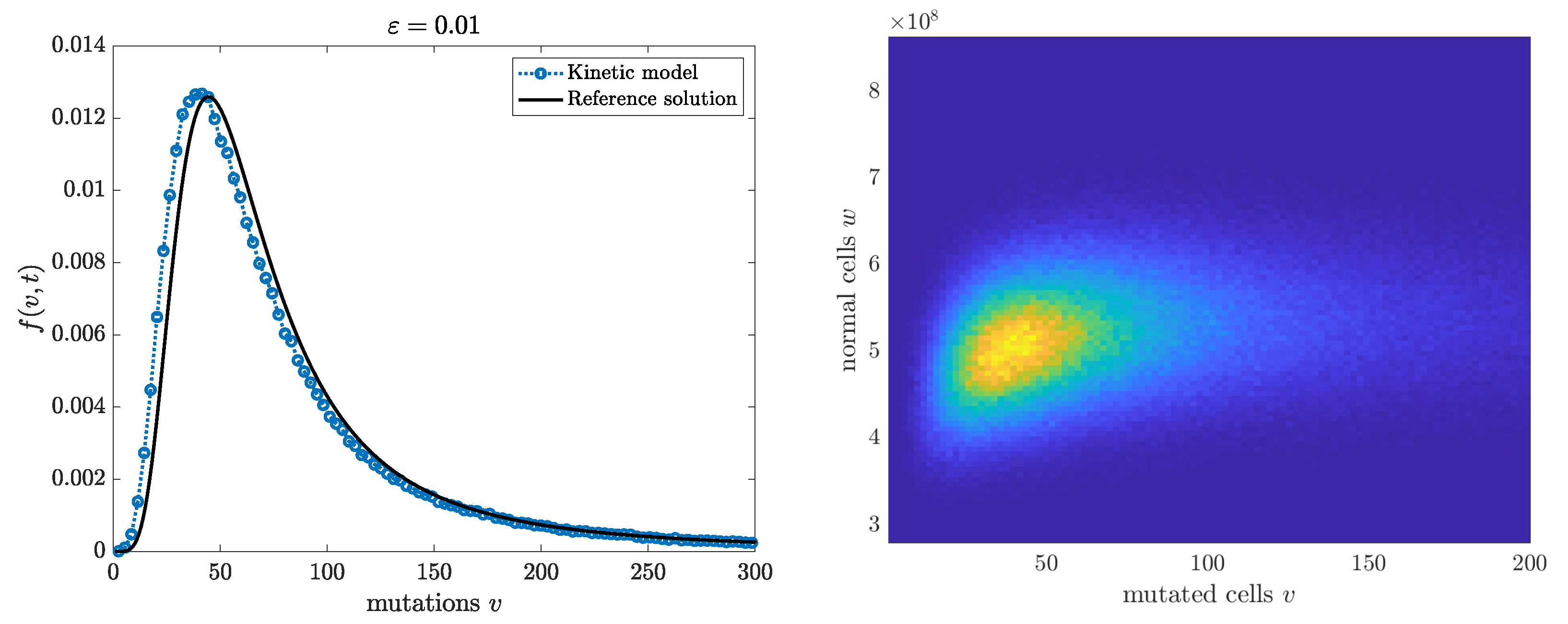
Finally, in Figure 3, we consider the same setting as in Figure 2 but now solving the kinetic model (47) under scaling (33) with $\epsilon =0.01$. The Monte Carlo method is similar to the one in Algorithm 1, except that additional independent Poisson samples must be used to generate the two-dimensional dynamics. We omit the details. We report both the marginal density of the mutants and the full two-dimensional kinetic solution. The good agreement of the marginal distribution of the mutants with the Lea-Coulson solution is evident.

5. Conclusions

Linear kinetic theory is a powerful tool for modeling many particle systems subject to elementary interactions. Among the various problems that can benefit from this methodology, successful attempts have been made in recent years to study the classical problem of mutation rates, pioneered by the Luria and Delbrück experiment. In this paper, following the work done in [19,20], we briefly presented the main building blocks that enable the construction of easy-to-handle mathematical models that use the relationships between elementary interactions to define the macroscopic behavior of the whole system. Theoretical results and numerical simulations showed how these models can be used to characterize the asymptotic distribution of mutant cells.

References

- Castellano, C.; Fortunato, S.; Loreto, V. Statistical physics of social dynamics. Rev. Mod. Phys. 2009, 81, 591–646. [Google Scholar] [CrossRef] [Green Version]
- Düring, B.; Matthes, D.; Toscani, G. A Boltzmann type approach to the formation of wealth distribution curves. Riv. Mat. Univ. Parma 2009, 1, 199–261. [Google Scholar] [CrossRef] [Green Version]
- Naldi, G.; Pareschi, L.; Toscani, G. Mathematical Modeling of Collective Behavior in Socio-Economic and Life Sciences; Birkhäuser: Boston, MA, USA, 2010. [Google Scholar]
- Pareschi, L.; Toscani, G. Interacting Multiagent Systems: Kinetic Equations & Monte Carlo Methods; Oxford University Press: Oxford, UK, 2013. [Google Scholar]
- Cercignani, C. The Boltzmann Equation and Its Applications; Applied Mathematical Sciences, 67; Springer: New York, NY, USA, 1988. [Google Scholar]
- Luria, S.E.; Delbrück, M. Mutations of bacteria from virus sensitivity to virus resistance. Genetics 1943, 28, 491–511. [Google Scholar] [CrossRef]
- Lea, D.E.; Coulson, C.A. The distribution of the numbers of mutants in bacterial populations. J. Genet. 1949, 49, 264–285. [Google Scholar] [CrossRef]
- Angerer, W.P. An explicit representation of the Luria-Delbrück distribution. J. Math. Biol. 2001, 42, 145–174. [Google Scholar] [CrossRef] [PubMed]
- Armitage, P. The statistical theory of bacterial populations subject to mutation. J. R. Statist. Soc. B 1952, 14, 1–40. [Google Scholar] [CrossRef]
- Bartlett, M.S. An Introduction to Stochastic Processes with Special Reference to Methods and Applications, 2nd ed.; Cambridge University Press: London, UK; New York, NY, USA, 1966. [Google Scholar]
- Crump, K.S.; Hoel, D.G. Mathematical models for estimating mutation rates in cell populations. Biometrika 1974, 61, 237–252. [Google Scholar] [CrossRef]
- Jones, M.E.; Thomas, S.M.; Rogers, A. Luria-Delbrück fluctuation experiments: Design and analysis. Genetics 1994, 136, 1209–1216. [Google Scholar] [CrossRef]
- Koch, A.L. Mutation and growth rates from Luria-Delbrück fluctuation tests. Mutat. Res. 1982, 95, 129–143. [Google Scholar] [CrossRef]
- Ma, W.T.; Sandri, G.v.H.; Sarkar, S. Analysis of the Luria and Delbrück distribution using discrete convolution powers. J. Appl. Prob. 1992, 29, 255–267. [Google Scholar] [CrossRef]
- Mandelbrot, B. A population birth-and-mutation process, I: Explicit distributions for the number of mutants in an old culture of bacteria. J. Appl. Prob. 1974, 11, 437–444. [Google Scholar] [CrossRef]
- Pakes, A.G. Remarks on the Luria-Delbrück distribution. J. Appl. Prob. 1993, 30, 991–994. [Google Scholar] [CrossRef] [Green Version]
- Stewart, F.M.; Gordon, D.M.; Levin, B.R. Fluctuation analysis: The probability distribution of the number of mutants under different conditions. Genetics 1990, 124, 175–185. [Google Scholar] [CrossRef] [PubMed]
- Zheng, Q. Progress of a half century in the study of the Luria–Delbrück distribution. Math. Biosci. 1999, 162, 1–32. [Google Scholar] [CrossRef] [PubMed] [Green Version]
- Kashdan, E.; Pareschi, L. Mean field dynamics and the continuous Luria–Delbrück distribution. Math. Biosci. 2012, 240, 223–230. [Google Scholar] [CrossRef] [Green Version]
- Toscani, G. A kinetic description of mutation processes in bacteria. Kinet. Relat. Models 2013, 6, 1043–1055. [Google Scholar] [CrossRef]
- Kendall, D.G. Stochastic processes and population growth. J. R. Stat. Soc. B 1949, 11, 230–264. [Google Scholar] [CrossRef]
- Sakamoto, S. Global solutions to an equation for mutation process in bacteria and its preservation of positive supports. J. Math. Anal. Appl. 2022, 507, 125771. [Google Scholar] [CrossRef]
- Bernardi, B.; Pareschi, L.; Toscani, G.; Zanella, M. Effects of vaccination efficacy on wealth distribution in kinetic epidemic models. Entropy 2022, 24, 216. [Google Scholar] [CrossRef] [PubMed]
- Chakraborti, A. Distributions of money in models of market economy. Int. J. Mod. Phys. C 2002, 13, 1315–1321. [Google Scholar] [CrossRef] [Green Version]
- Chakraborti, A.; Chakrabarti, B.K. Statistical mechanics of money: Effects of saving propensity. Eur. Phys. J. B 2000, 17, 167–170. [Google Scholar] [CrossRef] [Green Version]
- Chatterjee, A.; Chakrabarti, B.K.; Stinchcombe, R.B. Master equation for a kinetic model of trading market and its analytic solution. Phys. Rev. E 2005, 72, 026126. [Google Scholar] [CrossRef] [Green Version]
- Cordier, S.; Pareschi, L.; Toscani, G. On a kinetic model for a simple market economy. J. Stat. Phys. 2005, 120, 253–277. [Google Scholar] [CrossRef] [Green Version]
- Dimarco, G.; Pareschi, L.; Toscani, G.; Zanella, M. Wealth distribution under the spread of infectious diseases. Phys. Rev. E 2020, 102, 022303. [Google Scholar] [CrossRef]
- Drǎgulescu, A.; Yakovenko, V.M. Statistical mechanics of money. Eur. Phys. J. B 2000, 17, 723–729. [Google Scholar] [CrossRef] [Green Version]
- Düring, B.; Matthes, D.; Toscani, G. Kinetic equations modelling wealth redistribution: A comparison of approaches. Phys. Rev. E 2008, 78, 056103. [Google Scholar] [CrossRef] [Green Version]
- Hayes, B. Follow the money. Am. Sci. 2002, 90, 400–405. [Google Scholar] [CrossRef]
- Iglesias, J.R.; Gonçalves, S.; Pianegonda, S.; Vega, J.L.; Abramson, G. Wealth redistribution in our small world, Nonequilibrium statistical mechanics and nonlinear physics. Physica A 2003, 327, 12–17. [Google Scholar] [CrossRef]
- Slanina, F. Inelastically scattering particles and wealth distribution in an open economy. Phys. Rev. E 2004, 69, 046102. [Google Scholar] [CrossRef] [Green Version]
- Matthes, D.; Toscani, G. On steady distributions of kinetic models of conservative economies. J. Stat. Phys. 2008, 130, 1087–1117. [Google Scholar] [CrossRef]
- Bobylev, A.V. The theory of the spatially Uniform Boltzmann equation for Maxwell molecules. Sov. Sci. Rev. C 1988, 7, 111–233. [Google Scholar]
- Toscani, G. Kinetic models of opinion formation. Commun. Math. Sci. 2006, 4, 481–496. [Google Scholar] [CrossRef] [Green Version]
- Dimarco, G.; Pareschi, L.; Zanella, M. Micro-macro stochastic Galerkin methods for nonlinear Fokker-Plank equations with random inputs. arXiv 2022, arXiv:2207.06494. [Google Scholar]
- Pareschi, L.; Zanella, M. Structure preserving schemes for nonlinear Fokker–Planck equations and applications. J. Sci. Comput. 2018, 74, 1575–1600. [Google Scholar] [CrossRef]
- Zheng, Q. New algorithms for Luria–Delbrück fluctuation analysis. Math. Biosci. 2005, 196, 198–214. [Google Scholar] [CrossRef]
- Zheng, Q. Comparing mutation rates under the Luria–Delbrück protocol. Genetica 2016, 144, 351–359. [Google Scholar] [CrossRef] [PubMed]
- Gualandi, S.; Toscani, G.; Vercesi, E. A kinetic description of the body size distributions of species. Math. Mod. Meth. Appl. Sci. 2022, 32, 2853–2885. [Google Scholar] [CrossRef]
- Galton, F. Typical laws of heredity. Nature 1877, 15, 492–495. [Google Scholar]
- Galton, F. Natural Inheritance; Mcmillan & Co.: London, UK, 1889. [Google Scholar]
- Stigler, S.M. The History of Statistics: The Measurement of Uncertainty before 1900; Harvard University Press: Cambridge, MA, USA, 1986. [Google Scholar]
- Furioli, G.; Pulvirenti, A.; Terraneo, E.; Toscani, G. Fokker–Planck equations in the modelling of socio-economic phenomena. Math. Mod. Meth. Appl. Sci. 2017, 27, 115–158. [Google Scholar] [CrossRef] [Green Version]
- Iksanov, A. Renewal Theory for Perturbed Random Walks and Similar Processes; Probability and Its Applications; Springer: Berlin/Heidelberg, Germany, 2016. [Google Scholar]
- Bassetti, F.; Toscani, G. Explicit equilibria in a kinetic model of gambling. Phys. Rev. E 2010, 81, 066115. [Google Scholar] [CrossRef] [Green Version]
- Gabetta, E.; Toscani, G.; Wennberg, B. Metrics for probability distributions and the trend to equilibrium for solutions of the Boltzmann equation. J. Statist. Phys. 1995, 81, 901–934. [Google Scholar] [CrossRef]
- Zolotarev, V.M. Metric distances in spaces of random variables and their measures. Math. USSR-Sb 1976, 30, 373. [Google Scholar] [CrossRef]
- Zheng, Q. On Bartlett’s formulation of the Luria–Delbrück mutation model. Math. Biosci. 2008, 215, 48–54. [Google Scholar] [CrossRef]
- Knuth, D.E. The Art of Computer Programming; Addison Wesley: Reading, MA, USA, 1997; Volume 1. [Google Scholar]
- Marsaglia, G. The incomplete Γ function as a continuous Poisson distribution. Comput. Math. Appl. 1986, 12, 1187–1190. [Google Scholar] [CrossRef] [Green Version]
Figure 1.
Luria–Delbrück case. Distribution of mutant cells at with , for (left) and (right) in the kinetic model (18) under scaling (33), with . The reference solution is computed using Lemma 2 in [18].
Figure 2.
Lea–Coulson case. Distribution of mutant cells at with and for (left) and (right) in the kinetic model (18) under scaling (33), with , a Poisson process of mean . The reference solution is computed using Lemma 2 in [18] and numerical quadrature.
Disclaimer/Publisher’s Note: The statements, opinions and data contained in all publications are solely those of the individual author(s) and contributor(s) and not of MDPI and/or the editor(s). MDPI and/or the editor(s) disclaim responsibility for any injury to people or property resulting from any ideas, methods, instructions or products referred to in the content. |
© 2023 by the authors. Licensee MDPI, Basel, Switzerland. This article is an open access article distributed under the terms and conditions of the Creative Commons Attribution (CC BY) license (https://creativecommons.org/licenses/by/4.0/).
Share and Cite
MDPI and ACS Style
Pareschi, L.; Toscani, G. The Kinetic Theory of Mutation Rates. Axioms 2023, 12, 265. https://doi.org/10.3390/axioms12030265
AMA Style
Pareschi L, Toscani G. The Kinetic Theory of Mutation Rates. Axioms. 2023; 12(3):265. https://doi.org/10.3390/axioms12030265
Chicago/Turabian StylePareschi, Lorenzo, and Giuseppe Toscani. 2023. "The Kinetic Theory of Mutation Rates" Axioms 12, no. 3: 265. https://doi.org/10.3390/axioms12030265
Note that from the first issue of 2016, this journal uses article numbers instead of page numbers. See further details here.