A Proof of Chaos for a Seasonally Perturbed Version of Goodwin Growth Cycle Model: Linear and Nonlinear Formulations

Abstract

We show the existence of complex dynamics for a seasonally perturbed version of the Goodwin growth cycle model, both in its original formulation and for a modified formulation, encompassing nonlinear expressions of the real wage bargaining function and of the investment function. The need to deal with a modified formulation of the Goodwin model is connected with the economically sensible position of orbits, which have to lie in the unit square, in contrast to what occurs in the model’s original formulation. In proving the existence of chaos, we follow the seminal idea by Goodwin of studying forced models in economics. Namely, the original and the modified formulations of Goodwin model are described by Hamiltonian systems, characterized by the presence of a nonisochronous center, and the seasonal variation of the parameter, representing the ratio between capital and output, which is common to both frameworks, is empirically grounded. Hence, exploiting the periodic dependence on time of that model parameter we enter the framework of Linked Twist Maps. The topological results valid in this context allow us to prove that the Poincaré map, associated with the considered systems, is chaotic, focusing on sets that lie in the unit square, and also when dealing with the original version of the Goodwin model. Accordingly, the trademark features of chaos follow, such as sensitive dependence on initial conditions and positive topological entropy.

1. Introduction

In the last years of his research activity, Goodwin in [1] studied, by means of numerical experiments, what can be obtained by the superimposition of exogenous cycles to cycles endogenously generated by a model, focusing, in particular, on the one by Rössler [2], and concluding that, “At this point it becomes appropriate to consider the relevance, if any, that these forced models have to economics. The answer is not difficult to find: the economy consists of a very large number of separate and distinct parts, with the result that these parts are subject to continual exogenous forces. To begin with there are the individual national economies increasingly acted on by the movements of the world economy. Then within the economy there are various markets with dynamics particular to them. There is the annual solar cycle with its influence on various markets, for example the agricultural, the touristic, the fuel, and any number of others” ([1], pp. 121–123).

Taking inspiration from such considerations, we investigate the effect produced on the dynamics of both the original version and a modified formulation of his celebrated growth cycle model (see [3,4]) (The interested reader can find in [5] a survey on the vast literature about the Goodwin model, concerning possible extensions or modifications of the original setting, in [3,4]), by the exogenous periodic variation in one of the model parameters, the seasonal oscillation of which is empirically grounded.

We recall that the Goodwin model represents, in Goodwin’s own words, a “starkly schematized”, yet incisive, manner, the relationships between capitalists and workers. The need to deal with a modified formulation of the growth cycle model comes from the fact that the original formulation, proposed in [3,4], is not coherent. Indeed, despite the linearity of the real wage bargaining function and of the investment function, the original Goodwin model consists of two nonlinear differential equations of the Lotka–Volterra type, the variables of which are wage share in national income and proportion of labor force employed, which, by definition, cannot exceed unit. On the other hand, orbits of the Goodwin model can lie everywhere in the first quadrant, possibly outside the unit square (Goodwin was aware of this fact and, indeed, in ([3], p. 57), he wrote “Both u [wage share in national income] and v [employment proportion] must be positive and v must, by definition, be less than unity; u normally will be also but may, exceptionally, be greater than unity (wages and consumption greater than total product by virtue of losses and disinvestment)”). Some contributions, such as those by Desai et al. [6] and Harvie et al. [7], were devoted to fixing such an issue in an economically sensible manner. Nonetheless, as shown by Madotto et al. in [8], those works do not solve the problem with the orbit position, since the assumptions made in those two papers are not sufficient to guarantee that orbits lie inside the unit square. Hence, keeping the settings in [6,7] as a starting point, but taking into consideration the results obtained in [8], we deal here with a different reformulation of the Goodwin growth cycle model, which, in its outcomes, is consistent with the meanings of the variables and, in particular, with their admissible ranges. In more detail, in our revisitation of the model, in regard to the real wage bargaining function, we opt for the nonlinear formulation of the Phillips curve proposed by Phillips in [9], and considered, for example, in [6]. For the investment function, we deal with a similar nonlinear formulation, used in the simulative analysis performed in [8], and satisfying the conditions found in that work, so as to ensure that orbits lie in the feasible region. We stress that a nonlinear investment function is also grounded from an economic viewpoint, since, according to [10], followed by [11], it is suitable to encompass the description of a more flexible savings behavior with respect to its linear counterpart. Moreover, the nonlinear version of the Phillips curve [9] was initially considered by Goodwin, too, who then linearized that expression in its well-known model so as to obtain an approximation for it, “in the interest of lucidity and ease of analysis” ([3], p. 55) (see also [6], p. 2666). Still, the economic interpretation requires the real wage bargaining function to be increasing in the proportion of labor force employed, while the investment function has to be decreasing in wage share in the national income.

Since the modified formulation of the Goodwin model that we are going to analyze fulfills the conditions in [8], we know that, like the original framework in [3,4], it is still a Hamiltonian system, characterized by the presence of a global, nonisochronous center. Hence, in order to analytically show the dynamic consequences produced on its periodic orbits by the exogenous periodic variation in one of the model parameters, we use the Linked Twist Maps (LTMs, hereinafter) method, recently employed, for instance, in [12] to show the existence of complex dynamics in two evolutionary game theoretical contexts. In particular, we assume that the chosen parameter alternates in a periodic fashion between two different values, e.g., due to a seasonal effect, and this allows us to prove the existence of chaotic dynamics. In order to make our choice empirically grounded, we focus on the parameter that describes the ratio between capital and output, since, keeping the capital level constant, production is no doubt influenced by phenomena that are periodic in nature. We can, for instance, take into consideration the oscillatory behavior during the solar year of the energy price in electricity markets in consequence of the varying demand over the months, as investigated, for example, in [13,14], or the different supply in the agricultural commodity markets in various seasons. We stress, however, that the same assumption about a periodic variation between two different values made on any other model parameter would produce analogous results in terms of generated dynamics, since all parameters influence the center position (We remark that this is a sufficient, albeit not necessary, condition in order to apply the LTMs method whenever we deal with a nonisochronous center, as long as the switching times between the regimes described by the two different parameter values are large enough. As shown, for example, in [12,15], the LTMs technique can be used even when, in consequence of the periodic perturbation of one of the model parameters, the center position does not vary, but the shape of the orbits is modified in a suitable manner).

In order to explain the LTMs technique we need to recall, on the one hand, the original setting of linked twist maps, as studied, for instance, in [16,17,18], with the corresponding assumptions of smoothness, preservation of Lebesgue measure and monotonicity of the angular speed with respect to the radial coordinate, and, on the other hand, the Stretching Along the Paths (henceforth, SAP) method, developed in the planar case in [19,20] and extended to higher dimensional frameworks in [21]. The SAP method is a topological technique that allows the existence of fixed points, periodic points and chaotic dynamics for continuous maps that expand the arcs along one direction and that are defined on sets homeomorphic to the unit cube in Euclidean spaces. The context of LTMs represents a geometrical framework in which it is possible to employ the SAP method in view of proving, as done, for example, in [22,23], the presence of the trademark features of chaos, such as sensitive dependence on initial conditions and positive topological entropy. In more detail, by a Linked Twist Map we mean the composition of two twist maps, each acting on an annulus, with the two annuli linked together, i.e., crossing in the two-dimensional case along two (or more) planar sets homeomorphic to the unit square, that we call generalized rectangles. Since our approach is purely topological, different from that in [16,17,18], we just need a twist condition on the boundary of the two linked annuli, similar to what is required in the Poincaré-Birkhoff fixed point theorem.

As explained above, in the present paper, we are going to apply the LTMs method to the original and to the modified formulations of the Goodwin model, that, according to the findings in [8], are Hamiltonian systems with nonisochronous centers, the position of the center varying when the value of one of the model parameters changes. In particular, in both frameworks we act on the ratio between capital and output, since it is sensible to assume that it alternates, due to a seasonal effect, in a periodic fashion between two different levels, one of which may be seen as a perturbation of the other. In this manner, starting either from the original or the modified formulation of the Goodwin model, we obtain two conservative systems, the unperturbed and the perturbed ones, and for each system we can consider an annulus made of energy level lines. Under suitable conditions, the orbits the two annuli are linked together, crossing in two disjoint generalized rectangles. In our settings, the LTMs technique consists of finding two such linked annuli, having intersections containing chaotic sets. Their existence is established by applying the SAP method to the Poincaré map obtained as composition of the Poincaré maps associated with the unperturbed system and the perturbed one. This leads us to work with discrete-time dynamical systems. Like what has happened in other contexts in which the LTMs method was used (see e.g., [12,23]), our results about the existence of complex dynamics are robust with respect to small changes, in $L^1$ norm, in the coefficients of the considered settings.

We stress that the nonisochronicity of the center plays a crucial role in applying the SAP method, because it implies that the Poincaré maps produce a twist effect on the linked annuli, since the orbits composing them are run with a different speed. In this manner, the generalized rectangles, where the annuli meet, are increasingly deformed with the passing of time. Hence, if the regimes governed by the unperturbed system and by the perturbed one are sufficiently long-lasting, the Poincaré maps transform the generalized rectangles into spiral-like sets, that intersect the same generalized rectangles many times, so that the stretching property required by the SAP method, in order to guarantee the existence of chaotic sets inside the generalized rectangles, is fulfilled.

Regarding the nonisochronicity of the center in the settings that we analyze in this manuscript, for the original formulation proposed in [3,4], we rely on the classical results in [24,25] about the monotonicity of the period of orbits for the Lotka–Volterra predator–prey model with respect to the energy level, since the Goodwin growth cycle model is a special case of that more general framework. For the modified formulation of the Goodwin model that we take into account we instead make reference to the findings obtained in [8] about the period of small and large cycles for a wide class of Hamiltonian systems encompassing the one here considered. More precisely, although an exhaustive analysis of the period of the orbits does not seem to be easy to perform, as discussed in [8], due to the presence of singularities in the model, Madotto et al. proved, on the one hand, that the approximation of the period length of small cycles by means of the period of the linearized system is valid near the equilibrium point and, on the other hand, that the period length of large cycles, approaching the boundary of the feasible set, i.e., the unit square in our context, is arbitrarily high. In view of illustrating, by means of a concrete example, our main result about the existence of complex dynamics for the modified formulation of the Goodwin model, we numerically checked that the periods of the orbits coinciding with the inner and the outer boundaries of the linked annuli, considered in our example, did not coincide, finding, in particular, that the period of the orbits increased with the energy level, in analogy with the classical results in [24,25] for the original formulation of the Goodwin model. This is in agreement with the simulative experiments performed in [8] for the same setting that we investigate. Indeed, using a different notation, the framework that we study has been essentially proposed in (Section 5.3 in [8]) to illustrate the difficulties which arise when trying to prove that the period map connected with the general class of Hamiltonian systems analyzed in that paper is increasing, even if the detailed numerical simulations performed in [8] suggest that the period monotonicity holds true for the system that we consider.

Hence, our contribution is strongly based, on the one hand, on the results contained in [8] about the period of cycles of a suitable class of Hamiltonian systems. On the other hand, our work belongs to the research strand which, starting from [22,23], shows how to use the LTMs method to prove the existence of complex dynamics in various continuous-time settings (see e.g., [26,27,28]). In more detail, the paper that is closest to ours is [23], where the LTMs method was applied to investigate the dynamical effects produced by a periodic harvesting in the predator–prey model. Namely, the original formulation of the Goodwin growth cycle model is a special case of the Lotka–Volterra predator–prey model. However, our analysis does not coincide with that performed in [23], since, led by the economic argument about the ratio between capital and output explained above, we perturb in a periodic fashion a different parameter with respect to [23], and this produces a dissimilar effect on the center position. Moreover, orbits were run counterclockwise in [23], while they are run clockwise in the present framework, and this aspect also affects the proof of our result about LTMs, in which we need to count the laps completed by suitable paths around the centers.

In addition to the fact that the LTMs method has not been applied to the Goodwin model yet, two further reasons led us to deal with its original formulation in our investigation.

The first one is to provide robustness to the results that we obtain for the model modified formulation, which, indeed, in their general conclusions do not depend on the particular expression of the equations involved, as long as we enter the class of Hamiltonian systems considered in [8]. Only the kind of geometrical configuration for orbits in the phase plane, and, thus, the way to use the LTMs method, could vary according to the formulation of the model equations and on the basis of how they depend on the parameter that is periodically perturbed. We remark that different nonlinear expressions for the real wage bargaining function, and for the investment function, could be sensible, as well. Nonetheless, we chose two formulations that, in addition to having already been considered in the existing literature, satisfy the conditions found in [8], ensuring that the center is nonisochronous and that orbits lie in the feasible region, i.e., the unit square, since the state variables, being wage share in national income and proportion of labor force employed, can neither be negative, nor exceed unity.

The second reason for considering the Goodwin original formulation of the growth cycle model lies in the possibility of showing how to use the LTMs method to prove the existence of chaotic sets lying inside the unit square, despite the previously mentioned issue with the orbit position in the original Goodwin setting. Namely, the chaotic sets are contained in the detected pair of linked annuli, that jointly constitute an invariant set under the action of the Poincaré map obtained as composition of the Poincaré maps associated with the unperturbed system and the perturbed one, since each annulus, being made of periodic orbits, is invariant under the action of the Poincaré map describing the corresponding regime. Choosing linked together annuli contained in the unit square solves the problem. As our illustrative examples show, this can be done even when dealing with parameter configurations analogous to those considered in [6,7]. We stress that the issue with the orbit position did not occur in [23], since the variables in the original Lotka–Volterra model, describing the size of prey and predator populations, are not confined to lying in the unit square.

The remainder of the paper is organized as follows. In Section 2, we recall the original formulation of the Goodwin growth cycle model and we explain how to apply the LTMs method in such a context, highlighting the differences with [23]. In Section 3, we introduce the modified formulation of the Goodwin model, for which we check the existence of chaotic dynamics by means of the LTMs technique. In Section 4, we recall the definitions and the results connected with the LTMs method used in the preceding sections. In Section 5, we conclude. Appendix A contains the mathematical proof of our results, as well as some related comments.

2. The LTMs Method for the Goodwin Model Original Formulation

Following Goodwin’s seminal idea in [1], of studying forced models in economics, we apply the Linked Twist Maps (henceforth, LTMs) method, the main features of which are described in Section 4, to his celebrated growth cycle model, in order to show the effects produced on its dynamics by the exogenous periodic variation in one of the model parameters, the seasonal oscillation of which is empirically grounded.

We start by briefly recalling the model’s original formulation proposed in [3,4].

Denoting by $u\left(t\right)\in [0,1]$ the wage share in national income and by $v\left(t\right)\in [0,1]$ the employment proportion, the Goodwin model reads as

$$\left\{\begin{array}{c}{u}^{\prime }=u\left(-(\alpha +\chi )+\rho v\right)\hfill \\ \hfill \\ v^{\prime }=v\left(-(\alpha +\beta )+\frac{1-u}{\sigma }\right)\hfill \end{array}\right.$$

(1)

where all parameters are positive and, in particular, $\alpha$ is the exogenous labor productivity growth rate, $\beta$ is the exogenous labor force growth rate, $\sigma$ is the capital–output ratio, while $\chi$ and $\rho$ characterize the real wage growth rate, which is of the form $-\chi +\rho v.$, We stress that, rather than $\chi ,$ the symbol $\gamma$ is generally used in the Goodwin model. However, we preferred to save $\gamma$ to denote paths (see e.g., Definition 2) in agreement with the existing literature on the SAP method. The first equation in (1) derives from Goodwin’s linearized version of the Phillips curve [9] in real wages (see the first equation in (9) for its nonlinear formulation). We refer the interested reader to [6] for the derivation of the second equation, based on the assumptions that capitalists reinvest all profits and workers consume all wages, and to [6,7] for further details on the model.

Although state variables, due to their meanings, can neither be negative nor exceed unity, the latter condition is not guaranteed by (1). Namely, those equations describe a conservative system with closed orbits lying everywhere in the first quadrant of ${\mathbb{R}}^2$ and surrounding the center

$$P=\left(1-\sigma (\alpha +\beta ),\frac{\alpha +\chi }{\rho }\right).$$

We stress that P lies in the unit square when

$$\sigma <\frac{1}{\alpha +\beta },\alpha +\chi <\rho .$$

(2)

The origin $O=(0,0)$ is an equilibrium, being a saddle. As it is immediate to check, System (1) is a special case of the Lotka–Volterra predator–prey model (see e.g., [29])

$$\left\{\begin{array}{c}{x}^{\prime }=x\left(a-by\right)\hfill \\ \hfill \\ y^{\prime }=y\left(-c+dx\right)\hfill \end{array}\right.$$

(3)

where $u\left(t\right)$ corresponds to $y\left(t\right)$ and $v\left(t\right)$ corresponds to $x\left(t\right),$ even if $x\left(t\right)$ and $y\left(t\right)$ are not confined to lie in $[0,1],$ since they are non-negative variables describing the size of the prey and of the predator populations, respectively. In particular, as in [23], we focused only on $x\left(t\right)>0$ and $y\left(t\right)>0$, being therein interested in dynamic outcomes characterized by the coexistence between prey and predator. In what follows we confine our analysis to positive values of $u\left(t\right)$ and $v\left(t\right).$ Specifically, System (3) describes the twofold, at one time beneficial and detrimental, nature of the interactions between predators and preys. Similarly, the Goodwin model schematically represents the involved relationship between capitalists and workers, with the wage share in national income being the predator variable and the employment proportion being the prey.

Both (1) and (3) describe Hamiltonian systems. In the former case, orbit equations are given by

$$E(u,v)=\frac{u}{\sigma }-\left(\frac{1}{\sigma }-\alpha -\beta \right)log\left(u\right)+\rho v-(\alpha +\chi )log\left(v\right)=\ell ,$$

for some $\ell \ge {\ell }_0,$ where ${\ell }_0$ is the minimum energy level attained by $E(u,v)$ on the open unit square ${(0,1)}^2,$ i.e., ${\ell }_0=E\left(P\right).$ Notice that, under (2), the minimum level attained by $E(u,v)$ on ${(0,1)}^2$ coincides with the minimum level attained on ${(0,+\infty )}^2,$ since we assume that $P\in {(0,1)}^2.$ Moreover, the period of the orbits of System (1) increases with the energy level, due to the possibility of relying on the classical results in [24,25] on the monotonicity of the period of the orbits for the Lotka–Volterra predator–prey model in (3). On the other hand, contrary to what happens with System (3), orbits for System (1) are run clockwise, as the analysis of the phase portrait shows. This is due to the fact that, as observed above, comparing Systems (1) and (3), $u\left(t\right)$ corresponds to $y\left(t\right)$ and $v\left(t\right)$ corresponds to $x\left(t\right).$

While Goodwin investigated, by means of numerical experiments in [1], the dynamic outcomes that can be obtained by superimposing exogenous cycles to cycles endogenously generated by a model, we analytically show the effect produced on the periodic orbits of System (1) by the exogenous periodic variation in one of the model parameters. In view of making our choice empirically grounded, we focus on $\sigma ,$ i.e., the capital–output ratio, since, keeping the capital level constant, production is certainly influenced by phenomena that are periodic in nature. We can, for example, consider the oscillatory behavior during the solar year of the energy price in electricity markets in consequence of the varying demand over the months, or the different supply in the agricultural commodity markets in the various seasons. To fix ideas, we concentrate on the second phenomenon, since it is clear that north of the equator, for instance, in Europe and in the United States, supply in the agricultural commodity markets is larger from April to October than during the remaining part of the year. Hence, for the capital–output ratio $\sigma$ we can assume a periodic alternation between a higher value, that we call ${\sigma }^{\left(I\right)},$ referring to fall and winter, and a lower value, which may be seen as a perturbation of the former, that we call ${\sigma }^{\left(II\right)},$ referring to spring and summer (In regard to seasonal variations in demand and energy price in electricity markets, according to [14], which refers to [13], “Cycles and seasonality have for a long time been observed in electricity markets. There are hourly, daily, weekly, and seasonal fluctuations in prices and demand”. See also [30] for a seasonal electricity demand and pricing analysis). We stress, however, that a similar assumption about a periodic variation made on any other model parameter would produce analogous results in terms of generated dynamics, since all parameters affect, in some way, the center position.

Supposing then that the capital–output ratio alternates between ${\sigma }^{\left(I\right)},$ for $t\in [0,T^{\left(I\right)})$, and ${\sigma }^{\left(II\right)},$ for $t\in [T^{\left(I\right)},T^{\left(I\right)}+T^{\left(II\right)}),$ with ${\sigma }^{\left(I\right)}>{\sigma }^{\left(II\right)}$, and that the same alternation between the two regimes recurs with T-periodicity, where $T=T^{\left(I\right)}+T^{\left(II\right)},$ we can assume that we are dealing with a system with periodic coefficients of the form

$$\left\{\begin{array}{c}{u}^{\prime }=u\left(-\left(\alpha \right(t)+\chi (t\left)\right)+\rho \left(t\right)v\right)\hfill \\ \hfill \\ v^{\prime }=v\left(-(\alpha \left(t\right)+\beta \left(t\right))+\frac{1-u}{\sigma \left(t\right)}\right)\hfill \end{array}\right.$$

(4)

where

$$k\left(t\right)\equiv k,\mathrm{for} k\in \{\alpha ,\beta ,\chi ,\rho \},\mathrm{and} \sigma \left(t\right)=\left\{\begin{array}{cc}{\sigma }^{\left(I\right)}\hfill & \mathrm{for}t\in [0,T^{\left(I\right)})\hfill \\ \hfill \\ {\sigma }^{\left(II\right)}\hfill & \mathrm{for}t\in [T^{\left(I\right)},T)\hfill \end{array}\right.$$

(5)

with

$$0<{\sigma }^{\left(II\right)}<{\sigma }^{\left(I\right)}<\frac{1}{\alpha +\beta },\alpha +\chi <\rho$$

(6)

as a consequence of (2). The function $\sigma \left(t\right)$ is supposed to be extended to the whole real line by T-periodicity.

When the capital–output ratio takes value ${\sigma }^{\left(i\right)},$ and, thus, we are in the regime having dynamics governed by the system that we call $\left(i\right),$ the center coincides with $P^{\left(i\right)}=\left(1-{\sigma }^{\left(i\right)}(\alpha +\beta ),\frac{\alpha +\chi }{\rho }\right),$ for $i\in \{I,II\}.$ Notice that, passing from $P^{\left(I\right)}$ to $P^{\left(II\right)},$ the ordinate of the center does not change, while its abscissa rises. In regard to orbits, they are closed for both Systems $\left(I\right)$ and $\left(II\right),$ surrounding $P^{\left(I\right)}$ and $P^{\left(II\right)},$ respectively, and they are run clockwise. In the former case, orbits have equation

$$E^{\left(I\right)}(u,v)=\frac{u}{{\sigma }^{\left(I\right)}}-\left(\frac{1}{{\sigma }^{\left(I\right)}}-\alpha -\beta \right)log\left(u\right)+\rho v-(\alpha +\chi )log\left(v\right)=\ell ,$$

(7)

for some $\ell \ge {\ell }_0^{\left(I\right)},$ while, in the latter case, orbits have equation

$$E^{\left(II\right)}(u,v)=\frac{u}{{\sigma }^{\left(II\right)}}-\left(\frac{1}{{\sigma }^{\left(II\right)}}-\alpha -\beta \right)log\left(u\right)+\rho v-(\alpha +\chi )log\left(v\right)=h,$$

(8)

for some $h\ge h_0^{\left(II\right)},$ where ${\ell }_0^{\left(I\right)}$ and $h_0^{\left(II\right)}$ are the minimum energy levels attained by $E^{\left(I\right)}(u,v)$ and $E^{\left(II\right)}(u,v)$ on ${(0,1)}^2,$ respectively, i.e., ${\ell }_0^{\left(I\right)}=E^{\left(I\right)}\left(P^{\left(I\right)}\right)$ and $h_0^{\left(II\right)}=E^{\left(II\right)}\left(P^{\left(II\right)}\right).$

The sets ${\Gamma }^{\left(I\right)}(\ell )=\{(u,v)\in {(0,+\infty )}^2:E^{\left(I\right)}(u,v)=\ell \},$ for $\ell >{\ell }_0^{\left(I\right)},$ are simple closed curves surrounding $P^{\left(I\right)}$, while ${\Gamma }^{\left(II\right)}\left(h\right)=\{(u,v)\in {(0,+\infty )}^2:E^{\left(II\right)}(u,v)=h\},$ for $h>h_0^{\left(II\right)},$ are simple closed curves surrounding $P^{\left(II\right)}.$ We call an annulus around $P^{\left(I\right)}$ System $\left(I\right)$ any set ${\mathcal{C}}^{\left(I\right)}({\ell }_1,{\ell }_2)=\{(u,v)\in {(0,+\infty )}^2:{\ell }_1\le E^{\left(I\right)}(u,v)\le {\ell }_2\}$ with ${\ell }_0^{\left(I\right)}<{\ell }_1<{\ell }_2,$ having an inner boundary coinciding with ${\Gamma }^{\left(I\right)}\left({\ell }_1\right)$, and an outer boundary coinciding with ${\Gamma }^{\left(I\right)}\left({\ell }_2\right).$ Similarly, we call an annulus around $P^{\left(II\right)}$ System $\left(II\right)$ any set ${\mathcal{C}}^{\left(II\right)}(h_1,h_2)=\{(u,v)\in {(0,+\infty )}^2:h_1\le E^{\left(II\right)}(u,v)\le h_2\}$ with $h_0^{\left(II\right)}<h_1<h_2$, having an inner boundary coinciding with ${\Gamma }^{\left(II\right)}\left(h_1\right)$ and an outer boundary coinciding with ${\Gamma }^{\left(II\right)}\left(h_2\right).$ In particular, we are interested in annuli for Systems $\left(I\right)$ and $\left(II\right)$ contained in ${(0,1)}^2$, due to the meaning of variables u and $v.$ This configuration is achieved by choosing annuli whose outer (and consequently, inner) boundary set lies sufficiently close to the corresponding center, i.e., for low enough values of the energy levels ${\ell }_2>{\ell }_0^{\left(I\right)}$ and $h_2>h_0^{\left(II\right)}$ (see, e.g., Figure 1).

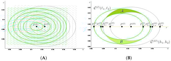
Figure 1. In (A) we draw in green some energy level lines associated with System $\left(I\right),$ surrounding $P^{\left(I\right)},$ and in gray some energy level lines associated with System $\left(II\right),$ surrounding $P^{\left(II\right)},$ together with the corresponding phase portrait. In (B), we illustrate Definition 1, showing how to obtain two linked together annuli by suitably choosing two level lines for each system. In particular, we call ${\mathcal{C}}^{\left(I\right)}({\ell }_1,{\ell }_2),{\mathcal{C}}^{\left(II\right)}(h_1,h_2)$ the two linked annuli, and $\mathcal{A}$ (colored in dark green), $\mathcal{B}$ (colored in light green) the two disjoint generalized rectangles obtained as the intersection between the two annuli.

In view of providing conditions of the energy levels that ensure that two annuli are linked together, thus, crossing in two disjoint generalized rectangles (see Section 4 for the corresponding definition), let us consider the straight line r joining $P^{\left(I\right)}$ and $P^{\left(II\right)},$ having equation $v=\left(\alpha +\chi \right)/\rho ,$ the ordering inherited from the horizontal axis, so that, given the points $R=(u_R,v^{*})$ and $S=(u_S,v^{*})$ belonging to $r,$ and hence with $v^{*}=\left(\alpha +\chi \right)/\rho ,$ it holds that $R⊲S$ (resp. $R⊴S$) if and only if $u_R<u_S$ (resp. $u_R\le u_S$). We are now in a position to introduce the following:

Definition 1. 

Given the annulus ${\mathcal{C}}^{\left(I\right)}({\ell }_1,{\ell }_2)$ around $P^{\left(I\right)}$ and the annulus ${\mathcal{C}}^{\left(II\right)}(h_1,h_2)$ around $P^{\left(II\right)},$ we say that they are linked together if

$$P_{2,-}^{\left(I\right)}⊲P_{1,-}^{\left(I\right)}⊴P_{2,-}^{\left(II\right)}⊲P_{1,-}^{\left(II\right)}⊴P_{1,+}^{\left(I\right)}⊲P_{2,+}^{\left(I\right)}⊴P_{1,+}^{\left(II\right)}⊲P_{2,+}^{\left(II\right)}$$

where, for $j\in \{1,2\}$, $P_{j,-}^{\left(I\right)}$ and $P_{j,+}^{\left(I\right)}$ denote the intersection points between ${\Gamma }^{\left(I\right)}\left({\ell }_j\right)$ and the straight line $r,$ with $P_{j,-}^{\left(I\right)}⊲P^{\left(I\right)}⊲P_{j,+}^{\left(I\right)},$ and, similarly, $P_{j,-}^{\left(II\right)}$ and $P_{j,+}^{\left(II\right)}$ denote the intersection points between ${\Gamma }^{\left(II\right)}\left(h_j\right)$ and $r,$ with $P_{j,-}^{\left(II\right)}⊲P^{\left(II\right)}⊲P_{j,+}^{\left(II\right)}.$

We stress that, for ${\ell }_j>{\ell }_0^{\left(I\right)}$ and $h_j>h_0^{\left(II\right)},j\in \{1,2\},$ the boundary sets ${\Gamma }^{\left(I\right)}\left({\ell }_j\right)$ and ${\Gamma }^{\left(II\right)}\left(h_j\right)$ intersect the straight line r in exactly two points, because $\{(u,v)\in {(0,+\infty )}^2:E^{\left(I\right)}(u,v)\le \ell \}$ and $\{(u,v)\in {(0,+\infty )}^2:E^{\left(II\right)}(u,v)\le h\},$ coinciding with the lower contour sets of the convex functions $E^{\left(I\right)}$ in (7) and $E^{\left(II\right)}$ in (8), are star-shaped for all $\ell >{\ell }_0^{\left(I\right)}$ and for every $h>h_0^{\left(II\right)},$ respectively. We refer the reader to Figure 1B for a graphical illustration of Definition 1.

We recall that a geometrical configuration analogous to that depicted in Figure 1B, except for the need for orbits to lie in the unit square, was found in [28] (cf. Figure 2 therein), where the LTMs method was applied to a periodically forced asymmetric second order ODE. However, in that case, the abscissa of the center decreased passing from the unperturbed regime to the perturbed one and the centers of the systems corresponding to the two regimes were located on the horizontal axis. Although both dissimilarities would not require the introduction of relevant differences in the statement and proof of the main result in [28] (cf. Theorem 1.2 therein), in adapting them to our framework, we provide a slightly more general (In (Theorem 1.2 in [28]) the special case of Proposition 1 with $m^{\left(I\right)}=m\ge 2$ and $m^{\left(II\right)}=1$ considered) version of (Theorem 1.2 in [28]) in Proposition 1, together with a complete proof (contained in the Appendix A) for the reader’s convenience.

To achieve such an aim, in addition to exploiting the tools recalled in Section 4 and, in particular, the stretching relation in (16), we need to introduce the Poincaré map $\Psi$ of System (4), which associates with any initial condition $(u_0,v_0)$ belonging to ${(0,+\infty )}^2$ the position at time T of the solution $\varsigma (·,(u_0,v_0))=(u(·,(u_0,v_0)),v(·,(u_0,v_0)))$ to (4) starting at time $t=0$ from $(u_0,v_0).$ In symbols, $\Psi :{(0,+\infty )}^2\to {(0,+\infty )}^2,(u_0,v_0)\mapsto \varsigma (T,(u_0,v_0)).$ The paper’s solutions are meant to be considered in the Carathéodory sense, being absolutely continuous and satisfying the corresponding system for almost every $t\in \mathbb{R}.$ We recall that a classical method to show the existence of periodic solutions for systems of first order ODEs with periodic coefficients is based on the search of the periodic points for the associated Poincaré map, under the assumption of uniqueness of the solutions for the Cauchy problems (cf. [31]). Notice that $\Psi$ is a homeomorphism on ${(0,+\infty )}^2$ and that it may be decomposed as $\Psi ={\Psi }^{\left(II\right)}\circ {\Psi }^{\left(I\right)},$ where ${\Psi }^{\left(I\right)}$ is the Poincaré map associated with System $\left(I\right)$ for $t\in [0,T^{\left(I\right)}]$ and ${\Psi }^{\left(II\right)}$ is the Poincaré map associated with System $\left(II\right)$ for $t\in [0,T^{\left(II\right)}].$ Moreover, since every annulus ${\mathcal{C}}^{\left(I\right)}({\ell }_1,{\ell }_2)$ around $P^{\left(I\right)}$ is invariant under the action of the map ${\Psi }^{\left(I\right)}$, being composed of the invariant orbits ${\Gamma }^{\left(I\right)}(\ell ),$ for $\ell \in [{\ell }_1,{\ell }_2]$, and, similarly, since every annulus ${\mathcal{C}}^{\left(II\right)}(h_1,h_2)$ around $P^{\left(II\right)}$ is invariant under the action of the map ${\Psi }^{\left(II\right)},$ it holds that every pair of linked together annuli is invariant under the action of the composite map $\Psi .$ In Proposition 1 we denote ${\tau }^{\left(I\right)}(\ell ),$ for all $\ell >{\ell }_0^{\left(I\right)},$ the period of ${\Gamma }^{\left(I\right)}(\ell ),$ i.e., the time needed by the solution ${\varsigma }^{\left(I\right)}(·,(u_0,v_0))$ to System $\left(I\right),$ starting from any $(u_0,v_0)\in {\Gamma }^{\left(I\right)}(\ell ),$ to complete one turn around $P^{\left(I\right)}$ moving along ${\Gamma }^{\left(I\right)}(\ell ),$ and by ${\tau }^{\left(II\right)}\left(h\right),$ for all $h>h_0^{\left(II\right)},$ the period of ${\Gamma }^{\left(II\right)}\left(h\right),$ i.e., the time needed by the solution ${\varsigma }^{\left(II\right)}(·,(u_0,v_0))$ to System $\left(II\right),$ starting from any $(u_0,v_0)\in {\Gamma }^{\left(II\right)}\left(h\right),$ to complete one turn around $P^{\left(II\right)}$ moving along ${\Gamma }^{\left(II\right)}\left(h\right).$ Orbits surrounding either $P^{\left(I\right)}$ or $P^{\left(II\right)}$ are run clockwise and ${\tau }^{\left(I\right)}(·)$ and ${\tau }^{\left(II\right)}(·)$ are monotonically increasing with the energy levels, since both features are fulfilled for System (1), as remarked above. Hence, for any annulus ${\mathcal{C}}^{\left(I\right)}({\ell }_1,{\ell }_2)$ around $P^{\left(I\right)}$ it holds that ${\tau }^{\left(I\right)}\left({\ell }_1\right)<{\tau }^{\left(I\right)}\left({\ell }_2\right),$ as well as for each annulus ${\mathcal{C}}^{\left(II\right)}(h_1,h_2)$ around $P^{\left(II\right)}$ it holds that ${\tau }^{\left(II\right)}\left(h_1\right)<{\tau }^{\left(II\right)}\left(h_2\right).$

Our result in regard to System (4) reads as follows:

Proposition 1. 

For any choice of the positive parameters $\alpha ,\beta ,\chi ,\rho ,{\sigma }^{\left(I\right)},$${\sigma }^{\left(II\right)}$ satisfying (6), given the annulus ${\mathcal{C}}^{\left(I\right)}({\ell }_1,{\ell }_2)$ around $P^{\left(I\right)},$ for some ${\ell }_0^{\left(I\right)}<{\ell }_1<{\ell }_2,$ and the annulus ${\mathcal{C}}^{\left(II\right)}(h_1,h_2)$ around $P^{\left(II\right)},$ for some $h_0^{\left(II\right)}<h_1<h_2,$ assume that they are linked together, calling $\mathcal{A}$ and $\mathcal{B}$ the connected components of ${\mathcal{C}}^{\left(I\right)}({\ell }_1,{\ell }_2)\cap {\mathcal{C}}^{\left(II\right)}(h_1,h_2).$ Then, for every $m^{\left(I\right)}\ge 1$ and $m^{\left(II\right)}\ge 1$ with $m=m^{\left(I\right)}{m}^{\left(II\right)}\ge 2$ there exist two positive constants $t^{\left(I\right)}=t^{\left(I\right)}(m^{\left(I\right)},{\tau }^{\left(I\right)}\left({\ell }_1\right),{\tau }^{\left(I\right)}\left({\ell }_2\right))$ and $t^{\left(II\right)}=t^{\left(II\right)}(m^{\left(II\right)},{\tau }^{\left(II\right)}\left(h_1\right),{\tau }^{\left(II\right)}\left(h_2\right))$ such that if $T^{\left(i\right)}>t^{\left(i\right)},$ for $i\in \{I,II\},$ the Poincaré map $\Psi ={\Psi }^{\left(II\right)}\circ {\Psi }^{\left(I\right)}$ of System (4) induces chaotic dynamics on m symbols in $\mathcal{A}$ and in $\mathcal{B},$ and all the properties listed in Theorem 1 are fulfilled for Ψ.

According to Proposition 1, whenever we have two linked together annuli related to Systems $\left(I\right)$ and $\left(II\right),$ if the switching times between the regimes described by those two systems are large enough, then the Poincaré map $\Psi ={\Psi }^{\left(II\right)}\circ {\Psi }^{\left(I\right)}$ induces chaotic dynamics on $m\ge 2$ symbols in the sets in which the two annuli intersect. As is clear from the proof of Proposition 1 (see the Appendix A), chaotic behavior is generated by the twist effect produced on the linked annuli by the different speeds with which their inner and outer boundary sets are run. Namely, after a long enough time, this twist effect suffices to make the image through ${\Psi }^{\left(I\right)}$ and ${\Psi }^{\left(II\right)}$ of the paths joining the inner and the outer boundary sets of the annuli spiral inside them and cross many times the intersection sets $\mathcal{A}$ and $\mathcal{B}$ between the linked annuli. In this manner, $\Psi$ satisfies the stretching relation described in Theorem 1 and, thus, all properties listed therein hold true for the composite Poincaré map.

We further notice that, under the assumptions in (6), which ensure that the centers of Systems $\left(I\right)$ and $\left(II\right)$ belong to the open unit square, when applying Proposition 1 to linked annuli, having inner and outer boundary sets lying sufficiently close to the centers, i.e., for low enough values of the energy levels ${\ell }_2>{\ell }_1>{\ell }_0^{\left(I\right)}$ and $h_2>h_1>h_0^{\left(II\right)}$, the chaotic invariant sets contained in $\mathcal{A}$ and in $\mathcal{B}$ lie in the open unit square, too. The same is true not only for the chaotic sets, but for a whole pair of linked annuli when the outer boundary sets ${\Gamma }^{\left(I\right)}\left({\ell }_2\right)$ and ${\Gamma }^{\left(II\right)}\left(h_2\right)$ are contained in ${(0,1)}^2$. Figure 1A shows this happening, where the parameter values are $\alpha =0.03,\beta =0.01,\chi =0.63,\rho =0.7,\sigma =3$. We stress that such parameter configuration is analogous to that considered in ([7], p. 77). The parameters in Figure 1A are similar to the those in ([6], p. 2668), where the authors set $\alpha =0.001,\beta =0.001,\chi =0.95,\rho =1,\sigma =3$. In the works mentioned, the symbol $\gamma$ was used instead of $\chi$. $\alpha =0.02,\beta =0.01,\chi =0.6,\rho =0.7,{\sigma }^{\left(I\right)}=3,{\sigma }^{\left(II\right)}=2.5,$ so that $P^{\left(I\right)}=(0.910,0.886)$ and $P^{\left(II\right)}=(0.925,0.886).$ In particular, as shown in Figure 1B, we obtain two linked together annuli ${\mathcal{C}}^{\left(I\right)}({\ell }_1,{\ell }_2)$ and ${\mathcal{C}}^{\left(II\right)}(h_1,h_2),$ contained in ${(0,1)}^2$ and crossing in the two disjoint generalized rectangles denoted by $\mathcal{A}$ and $\mathcal{B},$ e.g., for ${\ell }_1=1.0274,{\ell }_2=1.0276,h_1=1.0943,h_2=1.0946.$

Indeed, despite the previously recalled issue (see (2) and the lines above it) with the orbit position for the original formulation of the Goodwin model in (1), every annulus around $P^{\left(i\right)}$ for System $\left(i\right),$ with $i\in \{I,II\},$ being made of periodic orbits, is invariant under the action of the Poincaré map ${\Psi }^{\left(i\right)}.$ Consequently, each pair of linked annuli jointly constitutes an invariant set under the action of the composite Poincaré map $\Psi ={\Psi }^{\left(II\right)}\circ {\Psi }^{\left(I\right)},$ so that, even for System (1), the LTMs method allows the detection of complex dynamics that are consistent from an economic viewpoint.

Nonetheless, in Section 3 we introduce and analyze a modified formulation of the Goodwin growth cycle model (cf. (9)), whose orbits are all contained in the unit square, since the necessary and sufficient conditions found in [8] are fulfilled.

Before turning to that new framework, we stress that, like (Theorem 1.2 in [28]), Proposition 1 is also robust with respect to small changes, in $L^1$ norm, in the coefficients of System (4). Namely, from the proof of Proposition 1 it follows that, if $T^{\left(I\right)}$ and $T^{\left(II\right)}$ satisfy the conditions described in its statement, then, recalling System (4) and the definition of its coefficients in (5), there exists a positive constant $\epsilon$, such that the same conclusions of Proposition 1 hold true for the system

$$\left\{\begin{array}{c}{u}^{\prime }=u\left(-(\breve{\alpha }\left(t\right)+\breve{\chi }\left(t\right))+\breve{\rho }\left(t\right)v\right)\hfill \\ \hfill \\ v^{\prime }=v\left(-(\breve{\alpha }\left(t\right)+\breve{\beta }\left(t\right))+\frac{1-u}{\breve{\sigma }\left(t\right)}\right)\hfill \end{array}\right.$$

with $\breve{\alpha },\breve{\beta },\breve{\chi },\breve{\rho },\breve{\sigma }:\mathbb{R}\to \mathbb{R}$ being T-periodic functions with $T=T^{\left(I\right)}+T^{\left(II\right)},$ as long as

$${\int }_0^T\left|\breve{k}\left(t\right)-k\right|dt<\epsilon ,fork\in \{\alpha ,\beta ,\chi ,\rho \},$$

and

$${\int }_0^T\left|\breve{\sigma }\left(t\right)-\sigma \left(t\right)\right|dt={\int }_0^{T^{\left(I\right)}}\left|\breve{\sigma }\left(t\right)-{\sigma }^{\left(I\right)}\right|dt+{\int }_{T^{\left(I\right)}}^T\left|\breve{\sigma }\left(t\right)-{\sigma }^{\left(II\right)}\right|dt<\epsilon .$$

Due to the similar arguments that are needed in its proof, Proposition 2, i.e., the main result that we present in Section 3 about the Goodwin model modified formulation, is also robust with respect to small changes in the coefficients of System (13), in $L^1$ norm.

We conclude the present section by recalling that, in [23], the LTMs method was applied to the Lotka–Volterra System (3) under the assumption of a periodic harvesting, that perturbed the center position, causing an alternation for it between two points. However, since in [23] it was supposed that not only prey, but also predators decrease in number during the harvesting season, then both coordinates of the center change in that framework. Furthermore, orbits of System (3) are run counter-clockwise, rather than clockwise, like happens with the orbits of System (1), and, thus, the definition of the rotation number used in [23] does not coincide with that employed in the proof of Proposition 1 (cf. (A3) and (A4)). Those two differences between [23] and the above described context pushed us to provide a specific, complete presentation in the here analyzed setting of the LTMs method, and in its application to (1) in Proposition 1. Indeed, as recently shown in [12], the way in which the LTMs method can be used depends on the meaning attached to the variables and parameters of the considered model. Moreover, the detailed presentation of the LTMs method provided above is useful in view of Section 3, too, where it suffices for us to focus on the main steps, highlighting the dissimilarities with what we have already explained.

3. The Goodwin Model Modified Formulation

Rather than dealing with the linear expressions for the real wage bargaining function and for the investment function seen in Section 2, we now consider a modified formulation of such a setting, motivated by the issue with the orbit position in the original Goodwin model [3].

In regard to the real wage bargaining function, the most natural choice is given by the Phillips nonlinear specification in [9], even for real, rather than money, wages (cf. the first equation in System (9)). This was indeed what Goodwin initially assumed, before linearizing the Phillips curve so as to obtain the first equation in (1) as an approximation (see [3], p. 55). We recall that the nonlinear formulation of the Phillips curve in [9] was considered by, for example, by Desai et al., in [6], in their attempt to guarantee that the orbits of the growth cycle model lay inside the unit square. On the other hand, as shown by Madotto et al. in [8], the attempt by Desai et al. in [6] was not successful in fixing the problem with the orbit position because of their choice of the investment function (cf. Equation (10) in [6], page 2667), that describes a framework in which capitalists, depending on profitability, do not necessarily invest all profits. We stress that in [8] it is proven that even the modified version of the Goodwin model proposed by Harvie et al. in [7], does not ensure that orbits lie inside the unit square. In order to avoid similar issues, for the investment function we considered a nonlinear formulation (see the second equation in System (9)) satisfying the conditions found in [8], and that are recalled below, so as to guarantee that orbits lay in the feasible region. In more detail, for the investment function we dealt with the formulation used in the simulative analysis performed in (Section 5.3 in [8]). We underline that a nonlinear investment function is grounded also from an economic viewpoint, since, according to [10], followed by [11], it is suitable to describe more flexible savings behavior. Still, the economic interpretation requires the real wage bargaining function to increase in proportion to the labor force employed, while the investment function has decrease in the wage share in national income.

Since the modified formulation of the Goodwin model in (9), that we analyze satisfies the conditions in [8], we know that, like the original framework in [3,4], it is still a Hamiltonian system characterized by the presence of a global, nonisochronous center. Hence, in order to analytically show what the dynamic consequences produced on its periodic orbits by an exogenous periodic variation in one of the model parameters are, we to use the LTMs method. In particular, in view of making our parameter choice empirically grounded, due to the same argument explained in Section 2, we focus on the parameter that describes the ratio between capital and output, assuming that it alternates in a periodic fashion between two different values, due, for example, to a seasonal effect. This allows us to prove the existence of chaotic dynamics for System (13), i.e., the analog of System (4) obtained from (9). Nonetheless, as explained in Section 2, assuming a periodic variation on any other model parameter would lead to analogous conclusions about the system’s dynamic behavior, since the center position is influenced by all parameters.

In symbols, $u\left(t\right)\in [0,1]$ still denotes the wage share in national income and $v\left(t\right)\in [0,1]$ the employment proportion, our modified formulation of the Goodwin model reads as

$$\left\{\begin{array}{c}{u}^{\prime }=u\left(-(\chi +\alpha )+\frac{\rho }{{(1-v)}^{\delta }}\right)\hfill \\ \hfill \\ v^{\prime }=v\left(-(\alpha +\beta )+\frac{1}{\sigma }\left(c-\frac{\eta }{{(1-u)}^{\mu }}\right)\right)\hfill \end{array}\right.$$

(9)

where all parameters are positive and, in addition to $\alpha ,\beta$ and $\sigma$, that still describe the exogenous labor productivity growth rate, the exogenous labor force growth rate and the capital–output ratio, respectively, we have $\chi ,\rho$ and $\delta$ characterizing the real wage growth rate, which, in agreement with [9], is now in the form $-\chi +\frac{\rho }{{(1-v)}^{\delta }},$ while $c,\eta$ and $\mu$, together with $\sigma$, characterize the output growth rate, now formulated as $\frac{1}{\sigma }\left(c-\frac{\eta }{{(1-u)}^{\mu }}\right).$ In particular, as in the model’s original version in [3,4], it is assumed that capitalists reinvest all profits and workers consume all wages.

In addition to the origin $O=(0,0)$, which is still a saddle, the other equilibrium for System (9) is given by

$$\widehat{P}=\left(1-{\left(\frac{\eta }{c-\sigma (\alpha +\beta )}\right)}^{\frac{1}{\mu }},1-{\left(\frac{\rho }{\chi +\alpha }\right)}^{\frac{1}{\delta }}\right),$$

that belongs to the open unit square ${(0,1)}^2$ when

$$\sigma <\frac{c-\eta }{\alpha +\beta },\rho <\chi +\alpha ,\delta \ge 1,\mu \ge 1.$$

(10)

In order to ensure that $\widehat{P}$ is a global center for System (9), whose orbits lie in the square ${(0,1)}^2$, which is again the feasible region, due to the meaning of u and v, and in view of applying someof the results obtained in [8] on the period of orbits, we need to check the conditions described on p. 778 therein for the general system

$$\left\{\begin{array}{c}{u}^{\prime }=uf\left(u\right)\psi \left(v\right)\hfill \\ \hfill \\ v^{\prime }=-vg\left(v\right)\phi \left(u\right)\hfill \end{array}\right.$$

(11)

are fulfilled with the considered formulations of the real wage bargaining function and of the investment function, under the parameter assumptions in (10). When adapted to our framework, the conditions in [8] require that $f,g:(0,1)\to (0,+\infty )$ are continuous functions and that $\phi ,\psi :(0,1)\to \mathbb{R}$ are ${\mathcal{C}}^1$ maps with positive derivative on $(0,1),$ satisfying ${lim}_{u\to 0^{+}}\phi \left(u\right)\in (-\infty ,0),{lim}_{v\to 0^{+}}\psi \left(v\right)\in (-\infty ,0),{lim}_{u\to 1^{-}}\phi \left(u\right)>0,{lim}_{v\to 1^{-}}\psi \left(v\right)>0.$ All this is true in our context, since, setting $f\left(u\right)=1,\psi \left(v\right)=-(\chi +\alpha )+\frac{\rho }{{(1-v)}^{\delta }},$ $g\left(v\right)=1,$ $\phi \left(u\right)=(\alpha +\beta )-\frac{1}{\sigma }\left(c-\frac{\eta }{{(1-u)}^{\mu }}\right),$ holds that $f,g$ are continuous maps taking positive values only and $\phi ,\psi$ are ${\mathcal{C}}^1$ increasing maps in $(0,1),$ satisfying

$$\begin{array}{c}\underset{u\to 0^{+}}{lim}\phi \left(u\right)=\alpha +\beta -\frac{1}{\sigma }\left(c-\eta \right)\in (-\infty ,0),\hfill \\ \hfill \\ \underset{v\to 0^{+}}{lim}\psi \left(v\right)=-(\chi +\alpha )+\rho \in (-\infty ,0),\hfill \\ \hfill \\ \underset{u\to 1^{-}}{lim}\phi \left(u\right)=+\infty ,\underset{v\to 1^{-}}{lim}\psi \left(v\right)=+\infty \hfill \end{array}$$

under (10). Moreover, setting

$$A\left(u\right)=\int \frac{\phi \left(u\right)}{uf\left(u\right)}du=\int \frac{1}{u}\left((\alpha +\beta )-\frac{1}{\sigma }\left(c-\frac{\eta }{{(1-u)}^{\mu }}\right)\right)du$$

and

$$B\left(v\right)=\int \frac{\psi \left(v\right)}{vg\left(v\right)}dv=\int \frac{1}{v}\left(-(\chi +\alpha )+\frac{\rho }{{(1-v)}^{\delta }}\right)dv,$$

(12)

it holds that

$$\underset{u\to 0^{+}}{lim}A\left(u\right)=\underset{u\to 1^{-}}{lim}A\left(u\right)=\underset{v\to 0^{+}}{lim}B\left(v\right)=\underset{v\to 1^{-}}{lim}B\left(v\right)=+\infty ,$$

as required in [8], too. Hence, System (9) admits $\widehat{E}(u,v)=A\left(u\right)+B\left(v\right)$ as first integral, having $\widehat{P}$ as minimum point and, according to Theorem 3.1 in [8], its solutions are periodic and describe closed orbits, contained in the unit square, around $\widehat{P},$ that is a global center. In symbols, the orbit equations are then given by $\widehat{E}(u,v)=\ell$ for some $\ell \ge {\widehat{\ell }}_0$, where ${\widehat{\ell }}_0=\widehat{E}\left(\widehat{P}\right).$ Although an exhaustive analysis of the period of the orbits of System (9) seems not to be easy to perform, as discussed in [8], due to the presence of singularities in the model at $u=v=1$, Madotto et al. prove useful results about the period of small and large orbits for System (11).

On the one hand, they show that the approximation of the period length of small cycles by means of the period of the linearized system is valid near the equilibrium point (cf. Corollary 5.2 in [8]) and, on the other hand, they prove that the period length of large cycles, approaching the boundary of the feasible set, is arbitrarily high, in the case when f and g are, for instance, ${\mathcal{C}}^1$ functions on the open interval $(0,1),$ that are continuous in $0,$ too (cf. Theorem 5.3 in [8]), as happens in our framework. As previously mentioned, in view of its applying to System (9), or more precisely to (13) below, the method of the LTMs in some concrete scenarios (cf. Example 1) is used. Firstly, we perturb the center position by supposing that $\sigma$ alternates in a periodic fashion between two different levels, due to a seasonal effect, so as to obtain two conservative systems, for which we can find two linked together annuli and suitably choose an annulus made of energy level lines for each system. Then, we numerically check that the periods of the orbits coinciding with the inner and the outer boundaries of the considered linked annuli do not coincide. Actually, all the numerical simulations that we performed suggest the increasing monotonicity of the period of the orbits for System (9) with respect to the energy level, in analogy with the classical results in [24,25] for the original formulation of the Goodwin model, and in agreement with the numerical simulations reported in [8], even if, to the best of our knowledge, a rigorous proof of the period monotonicity for System (9) is not available in the literature. In fact, using a different, more abstract, notation, such a system was, essentially, proposed in (Section 5.3 in [8]) to illustrate the difficulties which arise when trying to prove that the period map connected with the general framework analyzed in that paper, described by (11), was increasing. The detailed numerical investigations performed in [8] suggest that the desired result holds true for the setting we dealt with, even if the period map had a different behavior in the four regions, called quadrants in [8], in which the feasible set ${(0,1)}^2$ is split by the horizontal and vertical lines passing through the center $\widehat{P}$. In more detail, Figures 3–7 in (Section 5.3 in [8]) show that the period is very long and increases with the energy level in the third quadrant, where both u and v assume low values, while it decreases in the first quadrant, and is not monotone in the second and fourth quadrants.

Let us assume that the capital–output ratio alternates in a T-periodic fashion between the same two positive values considered in Section 2, i.e., ${\sigma }^{\left(I\right)}>{\sigma }^{\left(II\right)},$ for the time intervals $t\in [0,T^{\left(I\right)})$ and $t\in [T^{\left(I\right)},T^{\left(I\right)}+T^{\left(II\right)})$, respectively (Indeed, the values of ${\sigma }^{\left(i\right)}$ and $T^{\left(i\right)},$ for $i\in \{I,II\},$ are determined by the economic features of the capital–output ratio, rather than by the model formulation. Nonetheless, considering different values for ${\sigma }^{\left(i\right)}$ and $T^{\left(i\right)}$ with respect to Section 2 would not affect the way in which the LTMs can be applied and the conclusions that can be drawn, as long as $0<{\sigma }^{\left(II\right)}<{\sigma }^{\left(I\right)}$ and $T^{\left(I\right)},T^{\left(II\right)}$ are large enough) with $T=T^{\left(I\right)}+T^{\left(II\right)},$ where ${\sigma }^{\left(II\right)}$ may be seen as a perturbation of ${\sigma }^{\left(I\right)}.$ We can then suppose that we are dealing with the following system with periodic coefficients

$$\left\{\begin{array}{c}{u}^{\prime }=u\left(-(\chi \left(t\right)+\alpha \left(t\right))+\frac{\rho \left(t\right)}{{(1-v)}^{\delta \left(t\right)}}\right)\hfill \\ \hfill \\ v^{\prime }=v\left(-(\alpha \left(t\right)+\beta \left(t\right))+\frac{1}{\sigma \left(t\right)}\left(c\left(t\right)-\frac{\eta \left(t\right)}{{(1-u)}^{\mu \left(t\right)}}\right)\right)\hfill \end{array}\right.$$

(13)

in which $\kappa \left(t\right)$ coincides with $\kappa ,$ for $\kappa \in \{\alpha ,\beta ,\chi ,c,\delta ,\eta ,\mu ,\rho \},$ $\sigma \left(t\right)$ is as in (5), assuming that it is extended to the whole real line by T-periodicity, and

$$0<{\sigma }^{\left(II\right)}<{\sigma }^{\left(I\right)}<\frac{c-\eta }{\alpha +\beta },\rho <\chi +\alpha ,\delta \ge 1,\mu \ge 1$$

(14)

as a consequence of (10).

Calling $\left(Mi\right),$ where M stands for “Modified (version of the Goodwin model)”, the system that we obtain when the capital–output ratio takes value ${\sigma }^{\left(i\right)},$ for $i\in \{I,II\},$ it is conservative, with the center coinciding with

$${\widehat{P}}^{\left(i\right)}=\left(1-{\left(\frac{\eta }{c-{\sigma }^{\left(i\right)}(\alpha +\beta )}\right)}^{\frac{1}{\mu }},1-{\left(\frac{\rho }{\chi +\alpha }\right)}^{\frac{1}{\delta }}\right).$$

(15)

Similar to what happened in Section 2, passing from ${\widehat{P}}^{\left(I\right)}$ to ${\widehat{P}}^{\left(II\right)}$, the abscissa of the center rises, while its ordinate does not change. The orbits of Systems $\left(MI\right)$ and $\left(MII\right)$ are closed, surrounding the corresponding center, and a straightforward analysis of the phase portrait shows that they run clockwise (cf. Figure 2A). Setting $A^{\left(i\right)}\left(u\right)=\int \frac{1}{u}\left((\alpha +\beta )-\frac{1}{{\sigma }^{\left(i\right)}}\left(c-\frac{\eta }{{(1-u)}^{\mu }}\right)\right)du,$ for $i\in \{I,II\},$ and, recalling the definition of $B\left(v\right)$ in (12), the orbits of Systems $\left(MI\right)$ and $\left(MII\right)$ have, respectively, equation ${\widehat{E}}^{\left(I\right)}(u,v)=A^{\left(I\right)}\left(u\right)+B\left(v\right)=\ell$ for some $\ell \ge {\widehat{\ell }}_0^{\left(I\right)}={\widehat{E}}^{\left(I\right)}({\widehat{P}}^{\left(I\right)})$ and ${\widehat{E}}^{\left(II\right)}(u,v)=A^{\left(II\right)}\left(u\right)+B\left(v\right)=h$ for some $h\ge {\widehat{h}}_0^{\left(II\right)}={\widehat{E}}^{\left(II\right)}({\widehat{P}}^{\left(II\right)}).$ The sets ${\widehat{\Gamma }}^{\left(I\right)}(\ell )$ and ${\widehat{\Gamma }}^{\left(II\right)}\left(h\right)$ can then be defined like in Section 2 for $\ell >{\widehat{\ell }}_0^{\left(I\right)}$ and $h>{\widehat{h}}_0^{\left(II\right)},$ just replacing $E^{\left(i\right)}$ with ${\widehat{E}}^{\left(i\right)}$ for $i\in \{I,II\},$ and they are still simple closed curves surrounding ${\widehat{P}}^{\left(I\right)}$ and ${\widehat{P}}^{\left(II\right)}$, respectively. We can proceed analogously to Section 2 in defining the annuli ${\widehat{\mathcal{C}}}^{\left(I\right)}({\ell }_1,{\ell }_2)$ around ${\widehat{P}}^{\left(I\right)},$ with ${\widehat{\ell }}_0^{\left(I\right)}<{\ell }_1<{\ell }_2,$ for System $\left(MI\right)$ and ${\widehat{\mathcal{C}}}^{\left(II\right)}(h_1,h_2)$ around ${\widehat{P}}^{\left(II\right)},$ with ${\widehat{h}}_0^{\left(II\right)}<h_1<h_2,$ for System $\left(MII\right),$ too. Notice, however, that, differing from Section 2, we do not need to consider energy levels close to ${\widehat{\ell }}_0^{\left(I\right)}$ and ${\widehat{h}}_0^{\left(II\right)}$ to have annuli for Systems $\left(MI\right)$ and $\left(MII\right)$ contained in ${(0,1)}^2,$ thanks to the above recalled results obtained in [8] (cf. in particular Theorem 3.1 therein). Due to the similar effect produced by a variation in $\sigma$ on the center position for Systems (1) and (9), the definition of linked together annuli in the new context is analogous to that introduced in Definition 1 as well, being based on the same ordering relation $⊲$, this time on the straight line $\widehat{r}$ joining ${\widehat{P}}^{\left(I\right)}$ and ${\widehat{P}}^{\left(II\right)}$, which has equation $v=1-{\left(\frac{\rho }{\chi +\alpha }\right)}^{\frac{1}{\delta }}.$ See Figure 2B for a graphical illustration of two linked annuli ${\widehat{\mathcal{C}}}^{\left(I\right)}({\ell }_1,{\ell }_2)$ and ${\widehat{\mathcal{C}}}^{\left(II\right)}(h_1,h_2)$ for System (13). We stress that in the present framework their boundary sets ${\widehat{\Gamma }}^{\left(I\right)}\left({\ell }_j\right)$ and ${\widehat{\Gamma }}^{\left(II\right)}\left(h_j\right),$ with $j\in \{1,2\},$ also intersect the straight line $\widehat{r}$ in exactly two points because the functions ${\widehat{E}}^{\left(I\right)}$ and ${\widehat{E}}^{\left(II\right)}$ are convex. Namely, their second derivative is non-negative under (14) because ${(1-z)}^{\nu }>(1-z(\nu +1)),\forall z\in [0,1],\forall \nu >0,$ where, in our case, $z\in \{u,v\}$ and $\nu \in \{\mu +1,\delta +1\},$ respectively.

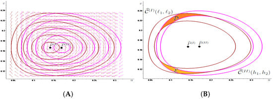
Figure 2. In (A) we draw in brown some energy level lines associated with System $\left(MI\right),$ around ${\widehat{P}}^{\left(I\right)},$ and in magenta some energy level lines associated with System $\left(MII\right),$ around ${\widehat{P}}^{\left(II\right)},$ also showing the corresponding phase portrait. In (B), we illustrate two linked together annuli, that we call ${\widehat{\mathcal{C}}}^{\left(I\right)}({\ell }_1,{\ell }_2)$ and ${\widehat{\mathcal{C}}}^{\left(II\right)}(h_1,h_2)$, obtained by suitably choosing two level lines for each system, as well as the two disjoint generalized rectangles $\mathcal{D}$ (colored in dark orange) and $\mathcal{E}$ (colored in light orange) where the annuli meet.

In view of stating our result about System (13) (cf. Proposition 2 below), for which we do not provide a proof, due to its similarity with the verification of Proposition 1, we introduce the Poincaré map $\widehat{\Psi }$ associated with System (13), that can be decomposed as $\widehat{\Psi }={\widehat{\Psi }}^{\left(II\right)}\circ {\widehat{\Psi }}^{\left(I\right)},$ where ${\widehat{\Psi }}^{\left(I\right)}$ is the Poincaré map associated with System $\left(MI\right)$ for $t\in [0,T^{\left(I\right)}]$ and ${\widehat{\Psi }}^{\left(II\right)}$ is the Poincaré map associated with System $\left(MII\right)$ for $t\in [0,T^{\left(II\right)}].$ Notice that every pair of linked together annuli for System (13), being made of energy level lines of Systems $\left(Mi\right),i\in \{I,II\},$ are invariant under the action of $\widehat{\Psi }.$ We denote by ${\widehat{\tau }}^{\left(I\right)}(\ell ),$ for all $\ell >{\widehat{\ell }}_0^{\left(I\right)},$ the period of ${\widehat{\Gamma }}^{\left(I\right)}(\ell ),$ and by ${\widehat{\tau }}^{\left(II\right)}\left(h\right),$ for all $h>{\widehat{h}}_0^{\left(II\right)},$ the period of ${\widehat{\Gamma }}^{\left(II\right)}\left(h\right),$ recalling that the period of an orbit is the time needed by the solution to the considered system, starting from a certain point of the orbit, to complete one turn around the corresponding center, moving around the orbit itself. As discussed above, the increasing monotonicity of ${\widehat{\tau }}^{\left(I\right)}(·)$ and ${\widehat{\tau }}^{\left(II\right)}(·)$ with the energy levels is suggested by the many simulative experiments that we performed and by the accurate numerical analysis in (Section 5.3 in [8]), but, to the best of our knowledge, a rigorous proof is not available in the literature. In the absence of a result showing that the period of orbits of Systems $\left(MI\right)$ and $\left(MII\right)$ always increases with energy levels, in Proposition 2 we assume that, given two linked together annuli for System (13), the period of the orbits composing their inner boundary is smaller than the period of the orbits composing their outer boundary. The main difference between Propositions 1 and 2 lies, indeed, in the necessity to exclude in the latter the fact that the period remains unchanged between the inner and outer boundaries of the linked annuli, since a variation in the periods is required for the Poincaré map to produce a twist effect on the annuli, which in turn allows the LTMs method to be applied. We recall that for System (4) such a variation was granted by the results in [24,25] on the monotonicity of the period of orbits for the Lotka–Volterra predator–prey model.

Proposition 2. 

For any choice of the positive parameters $\alpha ,\beta ,\chi ,c,\delta ,\eta ,\mu ,\rho ,$${\widehat{\sigma }}^{\left(I\right)},{\widehat{\sigma }}^{\left(II\right)}$ satisfying (14), given the annulus ${\widehat{\mathcal{C}}}^{\left(I\right)}({\ell }_1,{\ell }_2)$ around ${\widehat{P}}^{\left(I\right)},$ for some ${\widehat{\ell }}_0^{\left(I\right)}<{\ell }_1<{\ell }_2,$ and the annulus ${\widehat{\mathcal{C}}}^{\left(II\right)}(h_1,h_2)$ around ${\widehat{P}}^{\left(II\right)},$ for some ${\widehat{h}}_0^{\left(II\right)}<h_1<h_2,$ assume that they are linked together, calling $\mathcal{D}$ and $\mathcal{E}$ the connected components of ${\widehat{\mathcal{C}}}^{\left(I\right)}({\ell }_1,{\ell }_2)\cap {\widehat{\mathcal{C}}}^{\left(II\right)}(h_1,h_2).$ Then, if ${\widehat{\tau }}^{\left(I\right)}\left({\ell }_1\right)<{\widehat{\tau }}^{\left(I\right)}\left({\ell }_2\right),$${\widehat{\tau }}^{\left(II\right)}\left(h_1\right)<{\widehat{\tau }}^{\left(II\right)}\left(h_2\right),$ it holds that for every ${\hat{m}}^{\left(I\right)}\ge 1$ and ${\widehat{m}}^{\left(II\right)}\ge 1$ with $\widehat{m}={\widehat{m}}^{\left(I\right)}{\widehat{m}}^{\left(II\right)}\ge 2$ there exist two positive constants ${\widehat{t}}^{\left(I\right)}={\widehat{t}}^{\left(I\right)}({\hat{m}}^{\left(I\right)},$ ${\widehat{\tau }}^{\left(I\right)}\left({\ell }_1\right),{\widehat{\tau }}^{\left(I\right)}\left({\ell }_2\right))$ and ${\widehat{t}}^{\left(II\right)}={\widehat{t}}^{\left(II\right)}({\widehat{m}}^{\left(II\right)},{\widehat{\tau }}^{\left(II\right)}\left(h_1\right),{\widehat{\tau }}^{\left(II\right)}\left(h_2\right))$ such that if $T^{\left(i\right)}>{\widehat{t}}^{\left(i\right)},$ for $i\in \{I,II\},$ the Poincaré map $\widehat{\Psi }={\widehat{\Psi }}^{\left(II\right)}\circ {\widehat{\Psi }}^{\left(I\right)}$ of System (13) induces chaotic dynamics on $\widehat{m}$ symbols in $\mathcal{D}$ and in $\mathcal{E},$ and all the properties listed in Theorem 1 are fulfilled for $\widehat{\Psi }$.

We remark that the same conclusions in Proposition 2 would also hold true if the period of the inner boundary were larger (rather than smaller) with respect to the period of the outer boundary for at least one of the linked together annuli (Notice that, in those cases, the position of the boundary periods should be exchanged on the denominator of the fractions defining ${\widehat{t}}^{\left(I\right)}$ and/or ${\widehat{t}}^{\left(II\right)},$ which, respectively, coincide with those for $t^{\left(I\right)}$ and $t^{\left(II\right)}$ in the proof of Proposition 1 (see Appendix A), when replacing ${\tau }^{\left(i\right)}$ with ${\widehat{\tau }}^{\left(i\right)},$ for $i\in \{I,II\}.$) In Proposition 2 we chose to focus on the framework in which the period of the inner boundary is smaller than the period of the outer boundary for both the linked together annuli, because this is the scenario observed in the numerical experiments in (Section 5.3 in [8]), as well as in all the simulations that we performed. We find the same framework in Example 1, that concludes the present investigation of the modified version of the Goodwin model by illustrating a numerical context, in which Proposition 2 can be applied to show the existence of chaotic dynamics.

Notice that the parameter configuration considered in Example 1, and in its illustration in Figure 2, coincides with that used to draw Figure 1 in Section 2, as well as Figure A1 and Figure A2 in Appendix A, except for the parameters $c,\delta ,\eta$ and $\mu ,$ which were not present in the model’s original formulation in (1), and parameters $\chi$ and $\rho$, whose values have now been interchanged, in order to satisfy the second condition in (14), i.e., $\rho <\alpha +\chi ,$ guarantees that the ordinate of the centers for System (13) lies in the interval $(0,1).$ Such an hypothesis is incompatible with the last condition in (6), which played the same role in regard to the ordinate of the centers for System (4). Hence, some differences in the parameter values for the original and the modified versions of the Goodwin model need to be introduced, but we avoid adding unnecessary ones. In regard to the new parameters $\delta$ and $\mu ,$ we deal with the same values, i.e., $\delta =1$ and $\mu =1.2,$ used in the numerical simulations performed in (Section 5.3 in [8]) where, as already mentioned, the authors illustrate the issues which arise when trying to prove that the period map connected with System (9) is increasing, even if numerical evidence of such a conjecture for the above values of $\delta$ and $\mu .$ is found. We stress that the case $\delta =1$ was also considered in [6] (cf. p. 2668 therein), although in that framework the parameter $\mu$ was not present.

Example 1. 

We take $\alpha =0.02,\beta =0.01,\chi =0.7,\rho =0.6,{\sigma }^{\left(I\right)}=3,{\sigma }^{\left(II\right)}=2.5,c=0.45,\eta =0.3,\delta =1,\mu =1.2$ and recall (15), System $\left(MI\right)$ has a center in ${\widehat{P}}^{\left(I\right)}=(0.141,0.167)$ while System $\left(MII\right)$ has a center in ${\widehat{P}}^{\left(II\right)}=(0.170,0.167).$

As shown in Figure 2B, two linked together annuli ${\widehat{\mathcal{C}}}^{\left(I\right)}(e_1,e_2)$ and ${\widehat{\mathcal{C}}}^{\left(II\right)}(h_1,$ $h_2)$ can be obtained for $e_1=0.8657,e_2=0.8696,h_1=0.9865,h_2=0.9892,$ intersecting in the two disjoint generalized rectangles denoted by $\mathcal{D}$ and $\mathcal{E}.$ Software-assisted computations show that ${\widehat{\tau }}^{\left(I\right)}\left(e_1\right)\approx 111<{\widehat{\tau }}^{\left(I\right)}\left(e_2\right)\approx 114$ and ${\widehat{\tau }}^{\left(II\right)}\left(h_1\right)\approx 89<{\widehat{\tau }}^{\left(II\right)}\left(h_2\right)\approx 90.$ Hence, Proposition 2 guarantees the existence of chaotic dynamics for the Poincaré map $\widehat{\Psi }={\widehat{\Psi }}^{\left(II\right)}\circ {\widehat{\Psi }}^{\left(I\right)}$ associated with System (13) provided that the switching times ${\widehat{T}}^{\left(I\right)}$ and ${\widehat{T}}^{\left(II\right)}$ are large enough.

4. Recalling the Linked Twist Maps Method

In the present section we briefly recall the planar results of the Linked Twist Maps (LTMs) method that we used in Section 2 and Section 3, referring the interested reader to [22,23] for further details and to [32] for a three-dimensional version.

Although in the literature different assumptions, connected, for example, with measure theory and differential calculus, have been made on linked twist maps (see, e.g., [16,17,18]), we rely only on topological hypotheses. Indeed, given two annuli crossing along two (or more) planar sets homeomorphic to the unit square, by means of a linked twist map we mean the composition of two twist maps, each acting on one of the two annuli, which are homeomorphisms and that, similar to what is required in the Poincaré-Birkhoff fixed point theorem, produce a twist effect on the boundary sets of the two annuli, leaving them invariant. In the applications of LTMs illustrated in the present paper, we analyze Hamiltonian systems with a nonisochronous center, the position of which varies when modifying a parameter for which it is sensible to assume, due to a seasonal effect, a periodic alternation between two different values, one of which may be seen as a perturbation of the other. Thanks to this alternation, we obtain two conservative systems with a nonisochronous center and for each of them we can consider an annulus composed of energy level lines. Under certain conditions on the orbits, the two annuli cross in two generalized rectangles. The LTMs method consists in proving the presence of chaotic dynamics for the Poincaré map obtained as a composition of the Poincaré maps associated with the unperturbed system and with the perturbed one, which are homeomorphisms, by checking that they satisfy suitable stretching relations (cf. conditions $\left(C_F\right)$ and $\left(C_G\right)$ in Theorem 1, as well as (16)). We stress that the nonisochronicity of the centers is crucial in the above described procedure, because it implies that the orbits composing the linked annuli run with a different speed, so that the Poincaré maps produce a twist effect on the linked annuli, despite the invariance of closed orbits under the action of the Poincaré maps.

The stretching relation in (16) is the kernel of the Stretching Along the Paths (henceforth, SAP) method, i.e., the topological technique developed in the planar case in [19,20] and extended to the N-dimensional framework in [21], that allows the existence of fixed points, periodic points and chaotic dynamics for continuous maps that expand the arcs along one direction and that are defined on sets homeomorphic to the unit square. We start by introducing its main aspects, in order to be able to state Theorem 1, so that we can then more precisely describe what we mean by chaos.

We call path in ${\mathbb{R}}^2$ any continuous function $\gamma :[0,1]\to {\mathbb{R}}^2$ and we set $\overline{\gamma }:=\gamma \left([0,1]\right).$ By a generalized rectangle we mean a subset $\mathcal{R}$ of ${\mathbb{R}}^2$ homeomorphic to the unit square ${[0,1]}^2,$ through a homeomorphism $H:{\mathbb{R}}^2\supseteq {[0,1]}^2\to \mathcal{R}\subseteq {\mathbb{R}}^2.$ We also introduce the left and the right sides of $\mathcal{R},$ defined respectively as ${\mathcal{R}}_l^{-}:=H(\{0\}\times [0,1])$ and ${\mathcal{R}}_r^{-}:=H(\{1\}\times [0,1]).$ We call the pair

$$\tilde{\mathcal{R}}:=(\mathcal{R},{\mathcal{R}}^{-})$$

an oriented rectangle of ${\mathbb{R}}^2$, where ${\mathcal{R}}^{-}:={\mathcal{R}}_l^{-}\cup {\mathcal{R}}_r^{-}.$

The stretching along the paths relation for maps between oriented rectangles can then be defined as follows:

Definition 2. 

Given $\tilde{\mathcal{N}}:=(\mathcal{N},{\mathcal{N}}^{-})$ and $\tilde{\mathcal{O}}:=(\mathcal{O},{\mathcal{O}}^{-})$ oriented rectangles of ${\mathbb{R}}^2,$ let $F:\mathcal{N}\to {\mathbb{R}}^2$ be a function and $\mathcal{H}\subseteq \mathcal{N}$ be a compact set. We say that $(\mathcal{H},F)$ stretches $\tilde{\mathcal{N}}$ to $\tilde{\mathcal{O}}$ along the paths, and write

$$(\mathcal{H},F):\tilde{\mathcal{N}}\Bumpeq ⟶\tilde{\mathcal{O}},$$

(16)

if

-

F is continuous on $\mathcal{H};$

-

for every path $\gamma :[0,1]\to \mathcal{N}$ with $\gamma \left(0\right)\in {\mathcal{N}}_l^{-}$ and $\gamma \left(1\right)\in {\mathcal{N}}_r^{-}$ or with $\gamma \left(0\right)\in {\mathcal{N}}_r^{-}$ and $\gamma \left(1\right)\in {\mathcal{N}}_l^{-}$ there exists $[t^{\prime },t^{″}]\subseteq [0,1]$ such that $\gamma \left([t^{\prime },t^{″}]\right)\subseteq \mathcal{H},$ $F\circ \gamma \left([t^{\prime },t^{″}]\right)\subseteq \mathcal{O},$ with $F\left(\gamma \left(t^{\prime }\right)\right)\in {\mathcal{O}}_l^{-}$ and $F\left(\gamma \left(t^{″}\right)\right)\in {\mathcal{O}}_r^{-}$ or with $F\left(\gamma \left(t^{\prime }\right)\right)\in {\mathcal{O}}_r^{-}$ and $F\left(\gamma \left(t^{″}\right)\right)\in {\mathcal{O}}_l^{-}.$

We stress that to check the stretching relation in (16) we may need to consider paths $\gamma :[0,1]\to \mathcal{N}$ with $\gamma \left(0\right)\in {\mathcal{N}}_r^{-}$ and $\gamma \left(1\right)\in {\mathcal{N}}_l^{-}$; for example, when dealing with the composition of two functions (like in (17) where $\Phi :=G\circ F$), since the image through the first map of paths joining the opposite sides of a certain oriented rectangle $\tilde{\mathcal{M}}$ from left to right can connect the sides of ${\mathcal{N}}^{-}$ from right to left through a path that is the starting point of the second function. Nonetheless in the proof of Proposition 1, contained in Appendix A, it suffices for us to focus on paths joining the left and the right sides of the generalized rectangles where the functions start from, since we are not directly dealing with composite mappings. Namely, thanks to Theorem 1 (cf. in particular $\left(C_F\right)$ and $\left(C_G\right)$ therein), in order to check the existence of chaotic dynamics for the Poincaré map obtained as a composition of the Poincaré maps associated with the unperturbed Hamiltonian system and with the perturbed one, we can deal with the two Poincaré maps separately.

Theorem 1. 

Let $F:{\mathbb{R}}^2\supseteq D_F\to {\mathbb{R}}^2$ and $G:{\mathbb{R}}^2\supseteq D_G\to {\mathbb{R}}^2$ be continuous maps defined on the sets $D_F$ and $D_G,$ respectively. Let also $\tilde{\mathcal{N}}:=(\mathcal{N},{\mathcal{N}}^{-})$ and $\tilde{\mathcal{O}}:=(\mathcal{O},{\mathcal{O}}^{-})$ be oriented rectangles of ${\mathbb{R}}^2.$ Suppose that the following conditions are satisfied:

$\left(C_F\right)$

there are $\widehat{m}\ge 1$ pairwise disjoint compact sets ${\mathcal{H}}_0,\dots ,{\mathcal{H}}_{\widehat{m}-1}\subseteq \mathcal{N}\cap D_F$ such that ${\displaystyle ({\mathcal{H}}_i,F):\tilde{\mathcal{N}}\Bumpeq ⟶\tilde{\mathcal{O}},}$ for $i=0,\dots ,\widehat{m}-1;$

$\left(C_G\right)$

there are $\breve{m}\ge 1$ pairwise disjoint compact sets ${\mathcal{K}}_0,\dots ,{\mathcal{K}}_{\breve{m}-1}\subseteq \mathcal{O}\cap D_G$ such that ${\displaystyle ({\mathcal{K}}_j,G):\tilde{\mathcal{O}}\Bumpeq ⟶\tilde{\mathcal{N}},}$ for $j=0,\dots ,\breve{m}-1;$

$\left(C_m\right)$

$m:=\widehat{m}·\breve{m}\ge 2;$

$\left(C_{\Phi }\right)$

the composite map $\Phi :=G\circ F$ is injective on

$${\mathcal{H}}^{*}:=\bigcup _{\begin{array}{cc}& i=0,\dots ,\widehat{m}-1\hfill \\ & j=0,\dots ,\breve{m}-1\hfill \end{array}}{\mathcal{H}}_{i,j}^{\prime },with{\mathcal{H}}_{i,j}^{\prime }:={\mathcal{H}}_i\cap F^{-1}\left({\mathcal{K}}_j\right).$$

Then, setting

$$X_{\infty }:=\bigcap _{n=-\infty }^{\infty }{\Phi }^{-n}\left({\mathcal{H}}^{*}\right),$$

there exists a nonempty compact set

$$X\subseteq X_{\infty }\subseteq {\mathcal{H}}^{*}$$

in which the following properties are fulfilled:

$\left(i\right)$

X is invariant for Φ (that is, $\Phi \left(X\right)=X$);

$\left(ii\right)$

$\Phi {\upharpoonright }_X$ is semi-conjugate to the two-sided Bernoulli shift on m symbols, i.e., there exists a continuous map π from X onto ${\Sigma }_m:={\{0,\dots ,m-1\}}^{\mathbb{Z}},$ endowed with the distance

$$d({\mathbf{s}}^{\prime },{\mathbf{s}}^{″}):=\sum _{i\in \mathbb{Z}}\frac{|s_i^{\prime }-s_i^{″}|}{m^{\left|i\right|+1}},$$

for ${\mathbf{s}}^{\prime }={\left(s_i^{\prime }\right)}_{i\in \mathbb{Z}}$ and ${\mathbf{s}}^{″}={\left(s_i^{″}\right)}_{i\in \mathbb{Z}}\in {\Sigma }_m,$ such that the diagram

commutes, i.e., $\pi \circ \Phi =\sigma \circ \pi ,$ where $\sigma :{\Sigma }_m\to {\Sigma }_m$ is the Bernoulli shift defined by $\sigma \left({\left(s_i\right)}_i\right):={\left(s_{i+1}\right)}_i,\forall i\in \mathbb{Z};$

$\left(iii\right)$

the set $\mathcal{P}$ of the periodic points of $\Phi {\upharpoonright }_{X_{\infty }}$ is dense in X and the preimage ${\pi }^{-1}\left(\mathbf{s}\right)\subseteq X$ of every k-periodic sequence $\mathit{s}={\left(s_i\right)}_{i\in \mathbb{Z}}\in {\Sigma }_m$ contains at least one k-periodic point.

Furthermore, from conclusion $\left(ii\right)$ it follows that:

$\left(iv\right)$

$$h_{\mathrm{top}}(\Phi )\ge h_{\mathrm{top}}(\Phi {\upharpoonright }_X)\ge h_{\mathrm{top}}\left(\sigma \right)=log\left(m\right),$$

where $h_{\mathrm{top}}$ is the topological entropy;

$\left(v\right)$

there exists a compact invariant set $\Lambda \subseteq X$, such that ${\Phi |}_{\Lambda }$ is semi-conjugate to the two-sided Bernoulli shift on m symbols, topologically transitive and displaying sensitive dependence on initial conditions.

Proof. 

The crucial step consists in showing that

$$({\mathcal{H}}_{i,j}^{\prime },\Phi ):\tilde{\mathcal{N}}\Bumpeq ⟶\tilde{\mathcal{N}},i=0,\dots ,\widehat{m}-1,j=0,\dots ,\breve{m}-1.$$

(17)

See Theorem 3.1 in [33] for a verification of this property in more general spaces for the case $\widehat{m}=m\ge 2,\breve{m}=1.$ The condition in (17) is then easy to check (cf. Theorem 3.2 in [33] for a result analogous to ours, which follows as a corollary from Theorem 3.1 therein).

Recalling Definition 2.3 in [33], as a consequence of (17) it holds that $\Phi$ induces chaotic dynamics on m symbols in the set $\mathcal{N}.$ Conclusions $\left(i\right)$–$\left(v\right)$ then follow by Theorem 2.2 and by Footnote 4 in [34], where however, the case $m=2$ is considered. □

In the proof of Theorem 1, we mentioned the concept of a map inducing chaotic dynamics on $m\ge 2$ symbols on a set according to Definition 2.3 in [33]. For brevity’s sake, we do not go into detail, but stress that such a notion of chaos for the case $m=2$ bears a deep resemblance to the concept of chaos in the coin-tossing sense, discussed in [35]; however, being stronger than it. Namely, in addition to the requirement in [35] that every two-sided sequence of two symbols is realized through the iterates of the map, jumping between two disjoint compact subsets, Definition 2.3 in [33] also requires periodic sequences of symbols to be reproduced by periodic orbits of the map. We refer the interested reader to [34] for a comparison with other notions of chaos widely considered in the literature.

Notice that, in light of Definition 2.3 in [33], we can rephrase the statement of Theorem 1 above by saying that, when conditions $\left(C_F\right),\left(C_G\right),\left(C_m\right)$ and $\left(C_{\Phi }\right)$ therein are satisfied, the composite map $\Phi =G\circ F$ induces chaotic dynamics on $m\ge 2$ symbols in $\mathcal{N},$ knowing that from this fact all the properties listed in Theorem 1 hold true for $G\circ F,$ in regard to the existence of periodic points, too. We indeed used such reformulation of Theorem 1 in Section 2 and Section 3 (see, for instance, the statement of Propositions 1 and 2) when dealing with the composition of the Poincaré maps associated with unperturbed and with perturbed Hamiltonian systems.

5. Concluding Remarks

In the present work, following the seminal idea by Goodwin, in [1], that studying forced models in economics, obtained superimposing exogenous cycles to cycles endogenously generated by a model, we showed the existence of complex dynamics in both the original version of his celebrated growth cycle model (see [3,4]), and in a modified formulation of it, encompassing nonlinear expressions of the real wage bargaining function and of the investment function, already considered in the literature. In particular, in regard to the real wage bargaining function we dealt with the formulation proposed by Phillips in [9], while for the investment function we used an expression employed in [8]. The need to consider a modified formulation of the Goodwin model was motivated by the observation that its original version does not guarantee that orbits lie in the unit square, as they should, since the state variables are wage share in national income and proportion of labor force employed, which can neither be negative, nor exceed unity. We, however, underline that a nonlinear investment function is also grounded from an economic viewpoint, since it encompasses a description of more flexible savings behavior (cf. [10,11]). Goodwin initially considered the nonlinear version of the Phillips curve in [9], then linearized it so as to obtain an approximation “in the interest of lucidity and ease of analysis” ([3], p. 55).

Exploiting, in both the original and the modified settings, the periodic dependence on time of one of the model parameters and the Hamiltonian structure, characterized by the presence of a global nonisochronous center, we proved the presence of chaos for the Poincaré map associated with the considered systems by means of the Linked Twist Maps (LTMs) method, used, for example, in [22,23]. This led us to work with discrete-time dynamical systems. We stress that the obtained results, in their general conclusions, do not depend on the particular expression of the equations involved, as long as the class of Hamiltonian systems, considered in [8], is entered, for which it is therein proven that the center is nonisochronous and that orbits lie in the unit square. Concerning the necessary economic assumptions, we recall that the real wage bargaining function has to increase in proportion to the labor force employed, while the investment function has to decrease in wage share in national income.

Despite the issue with the orbit position in the original Goodwin model, even for that formulation we were able to prove the existence of chaotic sets lying in the unit square, thanks to the features of the LTMs method. Namely, the chaotic sets are located inside the generalized rectangular regions obtained as an intersection of the detected pair of linked annuli, that jointly constitute an invariant set under the action of the composite Poincaré map. Indeed each annulus, being made of periodic orbits, is invariant under the action of the Poincaré map describing the corresponding regime. Choosing linked together annuli contained in the unit square solves the problem. As our illustrative examples showed, this can be done even when dealing with parameter configurations analogous to those considered in [6,7].

The seminal idea by Goodwin in [1] of studying forced models in economics has been recently applied to a three-dimensional setting in [36], where the authors investigated the implications of describing exports as a function of the capital stock in the framework introduced in [37], which extended the original Goodwin model in [3] to an open economy setting that included the balance-of-payments constraint (BoPC) on growth. In more detail, in agreement with Goodwin’s insight, in [38], that Schumpeterian innovations requiring investment occur periodically, the authors in [36] added a nonlinear forcing term in the capital accumulation function and, referring to their Figure 5 on p. 266, say that “In this way, we obtain a scenario in which a non-linear system with a “natural” oscillation frequency interacts with an external “force” resulting in a chaotic attractor, as shown in Figure 5. The interplay between two or more independent frequencies characterizing the dynamics of the system is a well-known route to more complex behaviour”. It would then be interesting to check whether the LTMs method, or, more generally, the SAP (Stretching Along the Paths) technique, on which the LTMs method is based, could be employed in that setting, too, in order to rigorously prove the existence of complex dynamics.

In regard to three-dimensional applications of the LTMs technique, we recall [32] where, dealing with linked together cylindrical sets, the focus was on a 3D non-Hamiltonian system describing a predator–prey model with a Beddington–DeAngelis functional response in a periodically varying environment. Related to this, we also mention the 3D continuous-time non-Hamiltonian framework representing the Lotka–Volterra model with two predators and one prey in a periodic environment, considered in [39], for which the presence of chaos was shown by means of the SAP technique, without relying on LTMs geometry. Despite such dissimilarity in the employed method, the common starting point in the proofs of chaos for the frameworks analyzed in [32,39] is given by a study of the properties of the classical planar Lotka–Volterra system. Since, as we have seen, the Goodwin growth cycle model in [3,4] is a special case of the predator–prey setting, in view of proving the existence of chaotic phenomena for its 3D extension, proposed in [36], we could try to apply similar arguments to those used in [32,39]. We will investigate this possibility in a future work.

References

- Goodwin, R.M. Chaotic Economic Dynamics; Oxford University Press: Oxford, UK, 1990. [Google Scholar]
- Rössler, O.E. An equation for continuous chaos. Phys. Lett. 1976, 57A, 397–398. [Google Scholar] [CrossRef]
- Goodwin, R.M. A growth cycle. In Socialism, Capitalism and Economic Growth; Feinstein, C.H., Ed.; Cambridge University Press: Cambridge, UK, 1967; pp. 54–58. [Google Scholar]
- Goodwin, R.M. A growth cycle. In A Critique of Economic Theory; Hunt, E.K., Schwartz, J.G., Eds.; Penguin: Harmondsworth, UK, 1972; pp. 442–449. [Google Scholar]
- Veneziani, R.; Mohun, S. Structural stability and Goodwin’s growth cycle. Struct. Chang. Econ. Dynam. 2006, 17, 437–451. [Google Scholar] [CrossRef]
- Desai, M.; Henry, B.; Mosley, A.; Pemberton, M. A clarification of the Goodwin model of the growth cycle. J. Econ. Dyn. Control 2006, 30, 2661–2670. [Google Scholar] [CrossRef]
- Harvie, D.; Kelmanson, M.A.; Knapp, D.G. A dynamical model of business-cycle asymmetries: Extending Goodwin. Econ. Issues 2007, 12, 53–92. [Google Scholar]
- Madotto, M.; Gaudenzi, M.; Zanolin, F. A generalized approach for the modeling of Goodwin-type cycles. Adv. Nonlinear Stud. 2016, 16, 775–793. [Google Scholar] [CrossRef]
- Phillips, A.W.H. The relationship between unemployment and the rate of change of money wage rates in the United Kingdom, 1861–1957. Economica 1958, 25, 283–299. [Google Scholar]
- Flaschel, P. Some stability properties of Goodwin’s growth cycle. A critical elaboration. Z. Nationalökon. 1984, 44, 63–69. [Google Scholar] [CrossRef]
- Zhang, W. Cyclical economic growth—Re-examining the Goodwin model. Acta Math. Appl. Sin. 1991, 7, 114–120. [Google Scholar] [CrossRef]
- Pireddu, M. Chaotic dynamics in the presence of medical malpractice litigation: A topological proof via linked twist maps for two evolutionary game theoretic contexts. J. Math. Anal. Appl. 2021, 501, 125224. [Google Scholar] [CrossRef]
- Alvarez-Ramirez, J.; Escarela-Perez, R.; Espinosa-Perez, G.; Urrea, R. Dynamics of electricity market correlations. Physica A 2009, 388, 2173–2188. [Google Scholar] [CrossRef]
- Arango, S.; Larsen, E. Cycles in deregulated electricity markets: Empirical evidence from two decades. Energy Policy 2011, 39, 2457–2466. [Google Scholar] [CrossRef]
- Pascoletti, A.; Zanolin, F. From the Poincaré-Birkhoff fixed point theorem to linked twist maps: Some applications to planar Hamiltonian systems. In Differential and Difference Equations with Applications; Pinelas, S., Chipot, M., Dosla, Z., Eds.; Springer Proceedings in Mathematics & Statistics, 47; Springer: New York, NY, USA, 2013; pp. 197–213. [Google Scholar]
- Przytycki, F. Ergodicity of toral linked twist mappings. Ann. Sci. École Norm. Super. 1983, 16, 345–354. [Google Scholar] [CrossRef]
- Przytycki, F. Periodic points of linked twist mappings. Stud. Math. 1986, 83, 1–18. [Google Scholar] [CrossRef]
- Burton, R.; Easton, R.W. Ergodicity of linked twist maps. In Global Theory of Dynamical Systems, Proceedings of the International Conference Held at Northwestern University, Evanston, IL, USA, 18–22 June 1979; Lecture Notes in Mathematics, 819; Springer: Berlin, Germany, 1980; pp. 35–49. [Google Scholar]
- Papini, D.; Zanolin, F. On the periodic boundary value problem and chaotic-like dynamics for nonlinear Hill’s equations. Adv. Nonlinear Stud. 2004, 4, 71–91. [Google Scholar] [CrossRef]
- Papini, D.; Zanolin, F. Fixed points, periodic points, and coin-tossing sequences for mappings defined on two-dimensional cells. Fixed Point Theory Appl. 2004, 2004, 113–134. [Google Scholar] [CrossRef]
- Pireddu, M.; Zanolin, F. Cutting surfaces and applications to periodic points and chaotic-like dynamics. Topol. Methods Nonlinear Anal. 2007, 30, 279–319, Erratum in Topol. Methods Nonlinear Anal. 2009, 33, 395. [Google Scholar]
- Pascoletti, A.; Zanolin, F. Example of a suspension bridge ODE model exhibiting chaotic dynamics: A topological approach. J. Math. Anal. Appl. 2008, 339, 1179–1198. [Google Scholar] [CrossRef][Green Version]
- Pireddu, M.; Zanolin, F. Chaotic dynamics in the Volterra predator-prey model via linked twist maps. Opusc. Math. 2008, 28/4, 567–592. [Google Scholar]
- Rothe, F. The periods of the Volterra-Lotka system. J. Reine Angew. Math. 1985, 355, 129–138. [Google Scholar]
- Waldvogel, J. The period in the Lotka-Volterra system is monotonic. J. Math. Anal. Appl. 1986, 114, 178–184. [Google Scholar] [CrossRef]
- Burra, L.; Zanolin, F. Chaotic dynamics in a vertically driven planar pendulum. Nonlinear Anal. 2010, 72, 1462–1476. [Google Scholar] [CrossRef]
- Margheri, A.; Rebelo, C.; Zanolin, F. Chaos in periodically perturbed planar Hamiltonian systems using linked twist maps. J. Differ. Equ. 2010, 249, 3233–3257. [Google Scholar] [CrossRef][Green Version]
- Pascoletti, A.; Zanolin, F. Chaotic dynamics in periodically forced asymmetric ordinary differential equations. J. Math. Anal. Appl. 2009, 352, 890–906. [Google Scholar] [CrossRef]
- Braun, M. Differential Equations and Their Applications. An Introduction to Applied Mathematics, 4th ed.; Texts in Applied Mathematics, 11; Springer: New York, NY, USA, 1993. [Google Scholar]
- Lillard, L.A.; Acton, J.P. Seasonal electricity demand and pricing analysis with a variable response model. Bell J. Econ. 1981, 12, 71–92. [Google Scholar] [CrossRef]
- Krasnosel’skiĭ, M.A. The Operator of Translation along the Trajectories of Differential Equations; Translations of Mathematical Monographs, 19; American Mathematical Society: Providence, RI, USA, 1968. [Google Scholar]
- Ruiz-Herrera, A.; Zanolin, F. An example of chaotic dynamics in 3D systems via stretching along paths. Ann. Mat. Pura Appl. 2014, 193, 163–185. [Google Scholar] [CrossRef]
- Pascoletti, A.; Pireddu, M.; Zanolin, F. Multiple periodic solutions and complex dynamics for second order ODEs via linked twist maps. Electron. J. Qual. Theory Differ. Equ. 2008, 14, 1–32. [Google Scholar]
- Medio, A.; Pireddu, M.; Zanolin, F. Chaotic dynamics for maps in one and two dimensions: A geometrical method and applications to economics. Int. J. Bifurc. Chaos Appl. Sci. Eng. 2009, 19, 3283–3309. [Google Scholar] [CrossRef]
- Kirchgraber, U.; Stoffer, D. On the definition of chaos. Z. Angew. Math. Mech. 1989, 69, 175–185. [Google Scholar] [CrossRef]
- Dávila-Fernández, M.J.; Sordi, S. Path dependence, distributive cycles and export capacity in a BoPC growth model. Struct. Chang. Econ. Dyn. 2019, 50, 258–272. [Google Scholar] [CrossRef]
- Dávila-Fernández, M.J.; Sordi, S. Distributive cycles and endogenous technical change in a BoPC growth model. Econ. Model. 2019, 77, 216–233. [Google Scholar] [CrossRef]
- Goodwin, R. The nonlinear accelerator and the persistence of business cycles. Econometrica 1951, 19, 1–17. [Google Scholar] [CrossRef]
- Ruiz-Herrera, A.; Zanolin, F. Horseshoes in 3D equations with applications to Lotka-Volterra systems. NoDEA Nonlinear Differ. Equ. Appl. 2015, 22, 877–897. [Google Scholar] [CrossRef]
Disclaimer/Publisher’s Note: The statements, opinions and data contained in all publications are solely those of the individual author(s) and contributor(s) and not of MDPI and/or the editor(s). MDPI and/or the editor(s) disclaim responsibility for any injury to people or property resulting from any ideas, methods, instructions or products referred to in the content. |
© 2023 by the author. Licensee MDPI, Basel, Switzerland. This article is an open access article distributed under the terms and conditions of the Creative Commons Attribution (CC BY) license (https://creativecommons.org/licenses/by/4.0/).