Abstract
This paper assumes constant-stress accelerated life tests when the lifespan of the test units follows the XLindley distribution. In addition to the maximum likelihood estimation, the Bayesian estimation of the model parameters is acquired based on progressively Type-II censored samples. The point and interval estimations of the model parameters and some reliability indices under normal operating conditions at mission time are derived using both estimation methods. Using the Markov chain Monte Carlo algorithm, the Bayes estimates are calculated using the squared error loss function. Simulating the performances of the different estimation methods is performed to illustrate the proposed methodology. As an example of how the proposed methods can be applied, we look at two real-life accelerated life test cases. According to the numerical outcomes and based on some criteria, including the root of the mean square error and interval length, we can conclude that the Bayesian estimation method based on the Markov chain Monte Carlo procedure performs better than the classical methods in evaluating the XLindley parameters and some of its reliability measures when a constant-stress accelerated life test is applied with progressively Type-II censoring.
1. Introduction
Under normal operating conditions, the life test for high-reliability products is frequently time-consuming and expensive because it would take a considerable amount of time before acquiring a sufficient number of failures for the necessary analysis. To rapidly and cheaply gather data regarding such products under experimental time constraints, accelerated life tests (ALTs) are typically conducted. As part of the ALTs, stress variables are typically set, including the temperature, humidity, voltage, pressure, etc. To determine the life characteristics of the products, the data gathered throughout the accelerated testing can be analyzed and extrapolated to the normal operating conditions. Nelson [1], Meeker and Escobar [2], Tang [3] and Balakrishnan [4] have all offered substantial reviews on past findings on the topic of ALTs. One of the most often utilized tests in reliability engineering is the constant-stress ALT (CSALT). As a result of the CSALT, the researchers can divide the products into several groups and test each group at a specific level of stress. A constant level of stress is applied during the entire test duration, for example, to semiconductors and microelectronics, see Luo et al. [5]. There are usually two or more levels at which products are tested separately. For time saving, tests are even run simultaneously when possible. Numerous studies have been conducted on the statistical inferences for the CSALT under various lifetime distributions using both classical and Bayesian approaches. For instance, when the product lifetime follows the Weibull distribution, Wang [6] discussed the inference of the CSALT. Lin et al. [7] investigated the inferences of the CSALT for log-location-scale lifetime distributions. Sief et al. [8] studied the inference of the CSALT from the generalized half-normal distribution. Nassar et al. [9] investigated the estimation issues of the Lindley distribution with the CSALT. See also Hakamipour [10], Kumar et al. [11] and Wu et al. [12] for more detail.
Although the main objective of the ALTs is to shorten the period of the experiment, the researchers spend a lot of time waiting for all test units to fail. In such situations, it is crucial to deal with censored data. In general, censoring means that actual failure times are known for just a part of the units under investigation. The Type-I, Type-II, and progressive Type-II censoring (PT-IIC) schemes are the most frequently utilized censoring schemes in ALTs. The PT-IIC is more powerful than traditional Type-I and Type-I censoring which enables researchers to withdraw live units at various testing stages. Consider an experiment in which n identical units are put on a life test with a predetermined censoring plan , where m is the desired number of observed failures. For , at the time of the th failure, units from the remaining units are picked at random and removed from the test. Immediately, upon the occurrence of the last failure, all the remaining units are removed and the test is ended, i.e., In engineering experiments, some items must be removed for a more in-depth inspection or saved for use as test samples in future investigations. In this case, the PT-IIC plan naturally arises from such experiments. The test procedure of the CSALT in the presence of PT-IIC data will be discussed in detail in the next section. The PT-IIC scheme has received a lot of attention in the literature, for example, see Balakrishnan et al. [13], Balakrishnan and Lin [14], Chen and Gui [15], Wu and Gui [16], Dey et al. [17] and Alotaibi et al. [18]. A good introduction to the idea of progressive censoring as well as a leading review article is provided by Balakrishnan [19].
In view of the importance of the CSALT in rapidly ending the life test and the flexibility of the PT-IIC scheme over the conventional censoring schemes, our main aim in this paper is to investigate the estimation issues of the XLindley (XL) distribution when the data are gathered based on the PT-IIC plan with the CSALT. As far as we are aware, no work has yet addressed the CSALT model when PT-IIC data from the XL distribution are utilized. Although numerous studies investigated the estimation problems in the presence of CSALTs, few works studied the estimations of the reliability function (RF) and hazard rate function (HRF) under normal use conditions. In other words, the majority of the available studies considered only the estimation problems of the unknown parameters and say nothing regarding the estimation of the reliability indices under operating settings. Therefore, we think it is of interest to reliability engineers and other practitioners to identify the reliability measures under normal operating conditions in the case of the XL distribution. For more detail about the reliability estimation, see Wang et al. [20], Wang et al. [21] and Zhuang et al. [22]. In this study, the model parameters are estimated using both classical and Bayesian approaches and then after some reliability measures are evaluated under normal use conditions. Using the maximum likelihood method, as a classical approach, the maximum likelihood estimates (MLEs) of the different quantities are acquired and the associated approximate confidence intervals (ACIs) are also obtained. On the other hand, the Bayes estimates are investigated based on the squared error (SE) loss function. Due to the complex form of the joint posterior distribution, the Markov chain Monte Carlo (MCMC) procedure is implemented to obtain the required Bayes estimates as well as the Bayes credible intervals (BCIs). It is important to mention here that the derived estimators from the two estimation procedures cannot be theoretically compared because of their complicated structures. To get over this problem, we consider carrying out simulation research to compare the effectiveness of different estimators (point or interval) based on some statistical standards. Additionally, two examples are provided to illustrate how different approaches can be used. The simulation findings show that the MCMC procedure provides more accurate estimates of the model parameters as well as the RF and HRF under normal operating settings than those acquired based on the classical maximum likelihood method. Moreover, the real data analysis demonstrates that the XL distribution can be considered as a suitable model to fit constant-stress accelerated data sets, namely the oil of insulating fluid and transformer life-testing (TLT) data.
The article’s structure is as follows: A description of the model, the test method, and the assumptions are given in Section 2. The MLEs as well as the ACIs confidence intervals are covered in Section 3. The Bayes estimation and BCIs of the unknown parameters are provided in Section 4. Section 5 presents the findings of the simulation research that was carried out to assess the effectiveness of the various estimators. Finally, two data sets are examined in Section 6, and some concluding remarks are offered in Section 7.
2. Model Description, Test Procedure, and Assumptions
A special combination of the exponential and Lindley distributions, known as the XL distribution, was introduced by Chouia and Zeghdoudi [23] as a new variant of the Lindley distribution. They demonstrated that compared to other one-parameter models like the Xgamma, exponential, and Lindley distributions, the XL has greater flexibility. They demonstrated the flexibility and suitability of the XL distribution as a model for representing time-to-event data in the real world. In addition to having an increasing hazard function, which is typical in many fields, it also has a single parameter which considerably reduces the mathematical challenges in reliability estimation. Using an adaptive Type-II progressive hybrid censoring plan, Alotaibi et al. [24] addressed the estimation problems, including both classical and Bayesian methods, of the XL distribution. They also demonstrated that data sets from chemical engineering may be modeled using the XL distribution rather than some other classical distributions, including gamma and Weibull distributions. Assume that Y is an experimental unit’s lifetime random variable that follows the XL distribution with scale parameter . As a result, the probability density function (PDF), distribution function (DF), RF and HRF corresponding to Y are expressed, respectively, by
and
where .
2.1. Test Procedure
Under CSALT, assume that we have r accelerated stress levels , where the stress level under usual conditions is . Let be r subgroups created from a total of N identical test items, where . Assume that is the level of stress applied to the test units. The number of observed failure is fixed before starting the experiment with a prefixed progressive censoring plan , with the awareness that . At stress level , when the first failure, say , occurred, from the remaining surviving items, items are randomly removed. Similarly, at , items are randomly removed from the remaining items, and so on. At the time of the failure, say , all the remaining items are withdrawn. The PT-IIC data that were observed under the stress level were collected in this manner
2.2. Basic Assumptions
In the context of CSALT, the following assumptions are applied across the whole paper:
- Under the designed stress and the accelerated stress levels , the lifetime of test items follows the XL distribution with DF given by
- It is assumed that the life-stress model for the scale parameter of the XL distribution is log-linear, i.e.,where and are unknown parameters depending on the product’s characteristics and need to be estimated.
Based on the above assumptions, without the normalized constant, we can write the joint likelihood function of the unknown parameters and , given the observed data, as follows
where .
3. Maximum Likelihood Estimation
In this section, the MLEs of the unknown parameters and as well as the RF under designed stress are investigated. Moreover, the ACIs of these different parameters are discussed, employing the asymptotic properties of the MLEs. Using the aforementioned assumptions and by substituting the PDF and DF in the joint likelihood function presented in (5) by the PDF and DF of the XL distribution given by (1) and (2), respectively, we obtain
where and . The log-likelihood function of (6) is obtained as follows:
The MLEs of the model parameters, indicated by and , can be determined by solving the following non-linear likelihood equations which are obtained by setting the derivatives of the log-likelihood function in (7) with respect to and to zero
and
Because the solutions to the previous equations cannot be found in a closed form, the Newton–Raphson method is frequently employed in these circumstances to produce the appropriate MLEs and . Based on the estimated values and , we can obtain the MLEs of RF and HRF under normal operating conditions at mission time t, respectively, using the invariance property of the MLEs, as demonstrated below:
and
where
After having the point estimates for the various parameters, it is now interesting to construct the confidence intervals for the unknown parameters and , or any function of them, such as the RF and HRF. Here, we utilize the asymptotic normality of the MLEs to obtain the ACIs of the different parameters. According to Miller [25], the asymptotic distribution of the MLEs can be expressed as , where is the approximated variance–covariance matrix as presented below:
where
and
Therefore, for , the ACIs for and are provided by
where and are the main diagonal elements of (10) and is the upper percentile point of the standard normal distribution.
As a matter of fact, in order to establish the confidence bounds of the RF and HRF under normal operating conditions, we should first determine the variances of their estimators. Here, we approximate the necessary estimated variances of and using the delta method. To apply this approach, we need the first derivatives of RF and HRF with respect to the parameters and as follows:
and
Let and , evaluated at the MLEs of and . Then, the approximate estimated variances of and are obtained as follows:
Consequently, the ACIs of and can be constructed, respectively, as
4. Bayesian Estimation
When the sample size is large or the data are well collected, MLEs usually produce results that are reasonably accurate. However, when there is a lot of information missing from the data or the sample size is limited, the Bayesian paradigm produces a more precise inference. We discuss the Bayesian inference for the model parameters as well as the RF and HRF in this section. As we are aware, in a Bayesian investigation, the model parameters are generally treated as random variables that follow a set of predetermined prior distributions. On the basis of the prior knowledge and the observed data, it is then possible to acquire the posterior distributions of the model parameters and obtain the Bayes estimators as well. Keep in mind that the mean time to failure of the testing units is often lower in ALTs because of the stress conditions. In our case and for the XL distribution, one can see from Chouia and Zeghdoudi [23] that the mean is a decreasing function of the parameter . Under the log-linear model, this can be achieved for positive with any value for the parameter . This idea can be incorporated into the priors. We assume that the parameters are independent, where the parameter follows the normal distribution, which allows the parameter to be negative or positive. On the other hand, the parameter is assumed to follow the gamma distribution which is more flexible than other prior distributions and adapts the support of the parameter , i.e., and . Then, the joint prior distribution can be expressed as
where and are the hyperparameters. Equations (6) and (11), when combined, can provide the following as the joint posterior density function of and :
where A is the normalized constant given by
We can draw Bayes estimators with respect to parameters of interest and/or functions of parameters, say , using the SE loss function as follows:
Due to the ratio of two intractable integrals in (13), it appears that the Bayes estimator cannot be derived analytically. Due to this difficulty, the MCMC method is used, which does not require the computation of a normalizing constant. First, we must derive the conditional distributions of the parameters and to apply the MCMC technique. In light of (12), the following are the conditional posterior distributions of and , respectively,
and
It is noted that no analytical reduction to any well-known distributions can be achieved for the conditional distributions of and provided by (14) and (15), respectively. The main goal of MCMC algorithms is to generate samples from a given probability distribution. The “Monte Carlo” part of the method’s name is due to the sampling purpose, whereas the “Markov Chain” part comes from the kind of Markov chains. As a result, the Metropolis–Hastings (M-H) procedure is used to generate samples from these distributions in order to obtain the Bayes estimates and the BCIs. To implement the M-H procedure, we consider the normal distribution as the proposal distribution for both parameters. Thus, follow the steps listed below for the sample generation process:
To guarantee convergence and avoid the appeal of starting values, the first D generated samples are eliminated. In this case, we have , where , where . Based on large M, one can compute the Bayes estimates of based on the SE loss function as
where and . To obtain the BCI of , sort as , . Then, the BCI of the takes the form
5. Monte Carlo Simulations
To compare the behavior of the proposed point and interval estimators of the XL model parameter and its reliability characteristics RF and HRF , extensive simulation studies are conducted based on several combinations of (stress levels), (group size), (effective sample size) and (censoring pattern). We replicated the PT-IIC mechanism 1000 times when the true value of () is taken as (0.2, 0.5). At the same time, for the usual condition , the acquired estimates of and at time are evaluated when their actual values are taken as 0.9011 and 1.0438, respectively. Take 2 choices of stress levels , namely (1, 2) and (3, 5), , without loss of generality, and the failure percentages (FPs) are taken as to a specific amount m of each n. Moreover, for each setting, different progressive censoring mechanisms are considered as follows:
Once 1000 constant stress PT-IIC samples are collected, the maximum likelihood and Bayes estimates of , , (based on normal condition ), and along with their asymptotic and credible interval estimates are calculated. To perform the desired numerical evaluations, using R 4.2.2 software, we suggest to install both the ‘maxLik’ (proposed by Henningsen and Toomet [26]) and ’coda’ (proposed by Plummer et al. [27]) packages in order to carry out the maximum likelihood and Bayesian analysis.
Following the mean and variance criteria of the proposed density priors, we have chosen different sets of the prior parameters of and , called Prior[1]:(0.2, 5, 0.5, 1) and Prior[2]:(0.2, 1, 2.5, 5). These values are determined in such a way that the expected prior refers to the sample mean for the coefficient of interest. Alternatively, the hyperparameter values can also easily be specified using the past-sample technique. Following the M-H sampler described in Section 4, to obtain the Bayes point (or credible) estimates of , , , or , we simulated and samples.
To evaluate the convergence of the simulated MCMC draws of , , , or , when , and Scheme-1 (as an example), both the autocorrelation and trace convergence diagnostic plots are shown in Figure 1. It shows that the samples drawn from the Markov chain of all the unknown parameters are mixed adequately, and thus the calculated estimates are satisfactory.
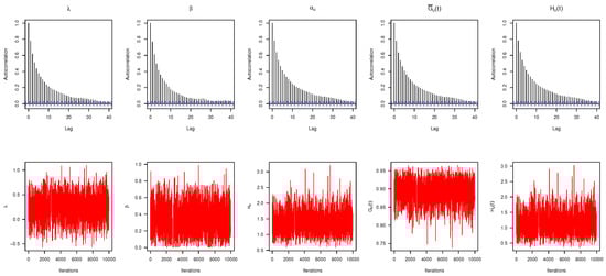
Figure 1.
Autocorrelation (top) and trace (bottom) plots for MCMC draws in Monte Carlo simulation.
Now, the comparison between the acquired point estimates of is made based on their root mean squared errors (RMSEs) and mean absolute biases (RABs), respectively, as
and
respectively, where is the calculated estimate at ith sample of .
Additionally, taking , the comparison between the acquired interval estimates of is made based on their average confidence lengths (ACLs) and coverage percentages (CPs) as
and
respectively, where is the indicator function, is the two-sided interval estimate. In a similar fashion, both point and interval estimates of , , and can easily be developed.
Nowadays, heat-map data visualization has become a popular tool for digital data representation as the value of each data point is indicated using specific colors. Therefore, all the simulated results (including the RMSE, MAB, ACL and CP) of , , , and are displayed by a heat-map tool in Figure 2, Figure 3, Figure 4, Figure 5 and Figure 6, respectively. Specifically, for Prior-1 (say P1) as an example, the Bayes estimates are mentioned as “BE-P1”, whereas the BCI estimates are mentioned as “BCI-P1”. All the numerical tables are also available as Supplementary Materials.
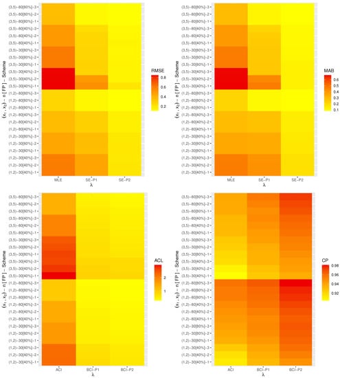
Figure 2.
Heat map for the simulation results of .
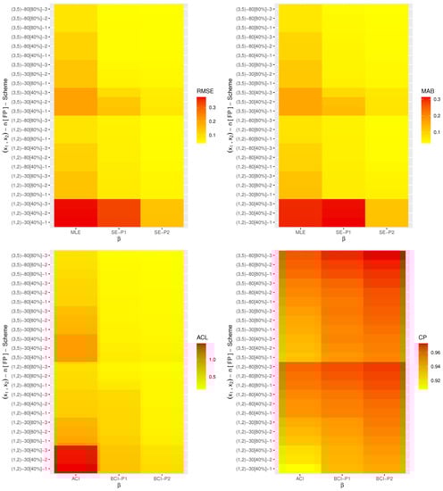
Figure 3.
Heat map for the simulation results of .
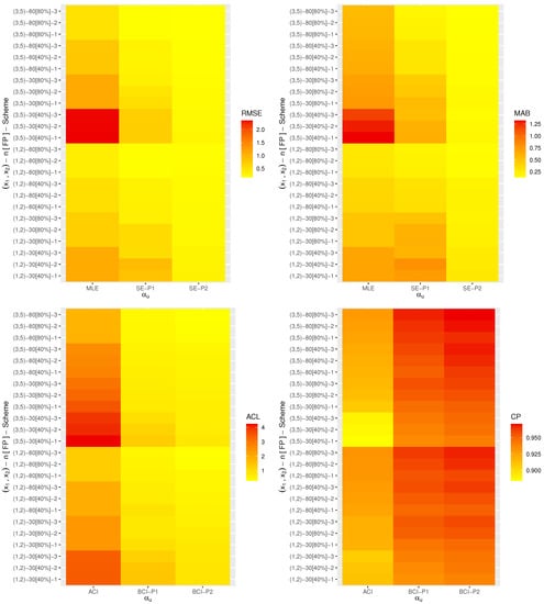
Figure 4.
Heat map for the simulation results of .
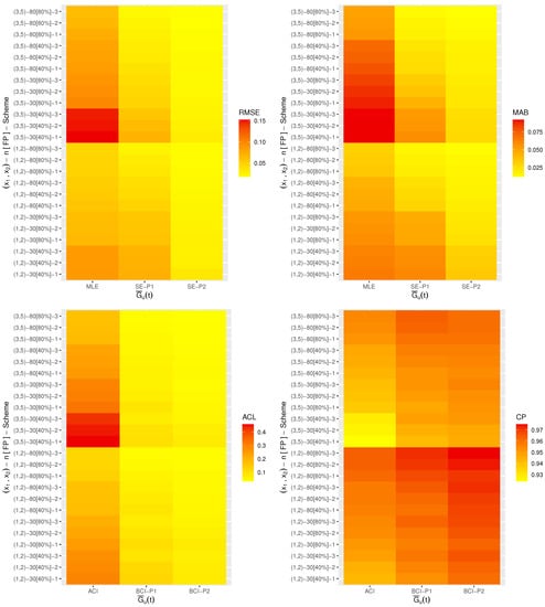
Figure 5.
Heat map for the simulation results of .
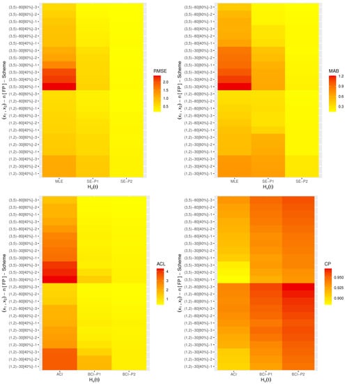
Figure 6.
Heat map for the simulation results of .
From Figure 2, Figure 3, Figure 4, Figure 5 and Figure 6, in terms of the lowest level of the RMSE, MAB and ACL values as well as the highest level of the CP values, we list the following conclusions:
- As a general comment, it is clear that the derived point (or interval) estimates of , , , or have a good performance.
- As n (or m or both) increases, all the calculated estimates provide better results and hold the consistency property. An equivalent observation is also reached when decreases.
- As increase, the following can be seen:
- The RMSEs and MRABs of all the estimates of increase while of they decrease.
- The RMSEs and MRABs of , and derived from the likelihood method increase while those derived from the Bayes method decrease.
- The ACLs of increase while of they decrease. The CPs of decrease while of they increase.
- The ACLs of , and obtained from the ACI method increase while those obtained from the BCI decrease. Regarding their CPs, the opposite result is noted.
- It is known that more accurate estimates will be obtained when the priors are used more accurately. Thus, for all settings, the MCMC estimates of , , , and provide more accurate results compared to those obtained from the likelihood method.
- Because the calculated variance of Prior[1] is higher than that associated with Prior[2], as anticipated, all the MCMC (or BCI) estimates using Prior[2] have more accurate results than the others, and both are better than those obtained from the MLE (or ACI) estimates.
- Comparing the proposed censoring schemes 1, 2 and 3, for both the point and interval estimates, it is observed that the proposed estimation procedures of , , , or perform better based on Scheme-3 (right censoring) than the others.
- To sum up, the simulation facts showed that the Bayes estimation method according to the M-H sampler for evaluating the XL parameters of life has a good performance and is recommended across different scenarios.
6. Real-Life Applications
To highlight the adaptability of acquired estimators to real-life situations, this section demonstrates two applications from the engineering field using two real data sets. These applications showed that the proposed estimation approaches work satisfactorily in practice.
6.1. Oil of Insulating Fluid
This application provides an analysis of the oil breakdown times (OBTs) of an insulating fluid subjected to various high test voltages. From Nelson [28], two data sets (in seconds) under different stress levels (kilovolt or kV) are considered; one is taken from 30 kV (normal use condition) and the other is taken from 32 kV (stress use condition). For computational convenience, each breakdown time point is divided by one hundred. So, the new transformed OBT data are presented in Table 1. Before addressing our inference, to check whether the XL model provides a significant fit to the OBT data or not, the Kolmogorov–Smirnov (KS) statistics along its p-value at a 5% significance level are considered. First, from Table 1, the MLE (standard error (SE)) of based on the normal and stress use OBT data sets is 1.5101(0.3835) and 2.6212(0.6097), respectively. Correspondingly, the KS (p-value) of the normal and stress use data sets is 0.203(0.682) and 0.309(0.089), respectively. It indicates, for both given stress levels, that the XL model fits the OBT data appropriately. Graphically, from Table 1, the fitted/empirical RFs as well as the probability–probability (PP) plots are plotted and shown in Figure 7. As we anticipated, Figure 7 shows that the proposed XL model provides a suitable fit to the OBT data sets.

Table 1.
Oil breakdown times of insulating fluid.
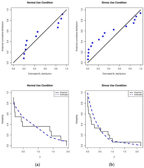
Figure 7.
Fitted RF (right) and PP (left) plots from OBT data. (a) Normal condition; (b) stress condition.
In this part, to see the usefulness of the derived point/interval estimators, several PT-IIC samples from the OBT data sets are obtained. From Table 1, taking different options of the effective samples and censoring plans , 3 artificial samples are created and listed in Table 2. Here, for brevity, the scheme is considered as . So, for each generated sample, the point estimates (including the maximum likelihood and Bayes estimates) and the interval estimates (including the asymptotic and credible interval estimates) of , , , and (for distinct time and the normal operating level ) are calculated. Obviously, we do not have any prior information about and ; thus, we set which means that the posterior density becomes quite close to the likelihood function. We also run the proposed MCMC procedure with a burn-in of 10,000 followed by 40,000 iterations. Thus, the Bayes point (or credible interval) estimates are evaluated. The initial values of and for beginning our iterations are taken as and , respectively. However, in Table 3, the point estimates (with their SEs) and the interval estimates (with their lengths) are presented. It shows that both the frequentist and Bayesian estimates are very close to each other while the latter performed better than the former with respect to the minimum standard errors and interval lengths. A similar behavior is also noted in the case of the interval estimates.
Table 2.
Various constant stress PC-T-II samples from OBT data.
Table 3.
Point and interval estimates from OBT data.
Moreover, to display the convergence of the generated Markovian chains, the histograms plot with the Gaussian kernel as well as the trace plot based on 40,000 MCMC variates are shown in Figure 8. Specifically, in Figure 8, the Bayes estimate of , , , and is highlighted by a solid line while their BCI bounds are highlighted by dashed lines. As a result, from Figure 8, it is observed that (i) the proposed estimates developed by the MCMC algorithm have sufficient convergence, (ii) the burn-in sample has enough size to eliminate the effect of the starting points and (iii) the density distribution of or is almost fairly symmetrical, of or it is positively skewed and of it is negatively skewed.
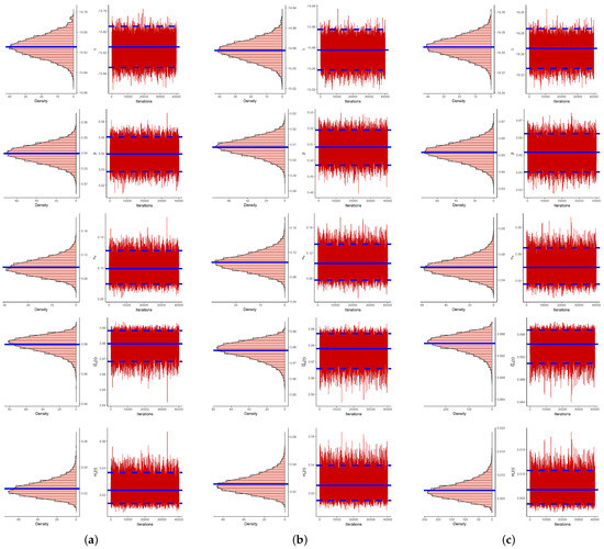
Figure 8.
Density (left) and trace (right) plot of , , , and from OBT data. (a) Sample 1; (b) Sample 2; (c) Sample 3.
6.2. Transformer Life-Testing
In this application, to show the usefulness of the proposed estimation approaches and to verify how our estimates work in practice, the failure times (in hours) of the TLT at high voltage are analyzed. These data were first given by Nelson [28] and later re-analyzed by Nassar et al. [9]. Under three accelerating stresses, 35.4, 42.2 and 46.7 kV, the TLT data sets were generated. In Table 4, each failure time in 35.4 kV (as normal use data) and 42.2 kV (as stress use data) is divided by 1000 for computational purposes, and the new transformed TLT data are presented. From Table 4, the MLE (SE) of based on the normal and stress use TLT data sets is 5.0778(1.7186) and 37.968(12.640), respectively. Next, the KS distance and its (p-value) from the normal and stress use TLT data sets is 0.185(0.901) and 0.287(0.374), respectively. This result is evidence that the XL model fits the TLT data sets well. On the other hand, in Figure 9, two plots, namely the fitted/empirical RFs and PP of the XL model, are displayed. It supports the same goodness-of-fit findings.
Table 4.
Failure times of transformer life-testing.
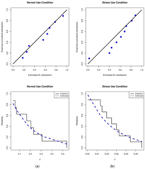
Figure 9.
Fitted RF (right) and PP (left) plots from TLT data. (a) Normal condition; (b) stress condition.
From Table 4, based on several choices of and , some artificial constant stress PT-IIC samples are generated and provided in Table 5. For each sample, in Table 6, the Bayes and maximum likelihood estimates along with their SEs as well as the 95% ACI/BCI estimates along with their lengths of , , , and (at and ) are calculated and provided. Just like our assumption about the prior parameters in Section 6.1, the acquired Bayes point/interval analyses are made. It is seen that the calculated point and interval estimates of , , , and , derived from the Bayes MCMC and likelihood estimation methods, are quite similar to each other. It also supports the same findings established in Table 3. To evaluate the behavior of 40,000 simulated Markovian chains of , , , or , for each generated sample in Table 4, the density and trace plots are shown in Figure 10. It indicates that the MCMC estimates converged adequately. It also depicts that the simulated posteriors of are distributed as fairly symmetric while of ( or ) and ( or ) they are distributed as negatively and positively skewed, respectively.
Table 5.
Various constant stress PC-T-II samples from TLT data.
Table 6.
Point and interval estimates from TLT data.
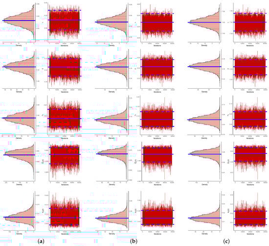
Figure 10.
Density (left) and trace (right) plot of , , , and from TLT data. (a) Sample 1; (b) Sample 2; (c) Sample 3.
As a summary, the numerical results developed from the OBT or TLT data revealed that the proposed XL model is useful for addressing the proposed inferential issues and is also beneficial for addressing the engineering problems.
7. Conclusions and Future Work
A statistical analysis of constant-stress accelerated life tests for the XLIndley distribution based on progressive Type-II censoring is investigated in this article. Even though there have been many studies looking into estimating problems when constant-stress accelerated life tests are present, there have been relatively few studies looking into the estimation of reliability and hazard rate functions in the context of normal use conditions. To fill this gap, we utilized classical and Bayesian inferential approaches to estimate the unknown parameters and reliability measures under normal use situations. Based on the maximum likelihood approach, the point estimates and the approximate confidence intervals based on the asymptotic normality of the maximum likelihood estimators are obtained. The squared error loss function is used in the Bayesian technique to derive the Bayes estimates. The Markov chain Monte Carlo approach is employed to obtain the Bayes estimates and the Bayes credible intervals of the unknown parameters due to the joint posterior distribution’s complex expression. The effectiveness of the various estimation techniques is demonstrated through a simulation study, and the applicability of the different estimators is verified through the analysis of two data sets from accelerated life tests. Based on the root mean square error, absolute bias and interval length of the estimates, the numerical results show that the Bayes estimates, whether point or interval, perform quite well. It is observed that the various estimates based on the right censoring scheme perform better than other censoring schemes. Moreover, the accuracy of the Bayes estimates increases as the prior distribution’s variance decreases. In general, when prior knowledge about the unknown parameters is available, the Bayes estimates outperform the maximum likelihood method. It is preferable to utilize the classical method when there is no information about the unknown parameters because the Bayesian method requires more calculation time. On future work, one can perform the same estimation procedures for the XLindley distribution described in the current study based on adaptive progressively censored samples. Referring to Opheim and Roy [29] and Avdović and Jevremović [30], the concepts of these two papers can be extended to test the XLindley distribution empirically by providing cut-off values for the required number of samples to attain predetermined nominal significance levels.
Supplementary Materials
The following supporting information can be downloaded at: https://www.mdpi.com/article/10.3390/axioms12040352/s1, Table S1: Average estimates (1st column), RMSEs (2nd column) and MABs (3rd column) of ; Table S2: Average estimates (1st column), RMSEs (2nd column) and MABs (3rd column) of ; Table S3: Average estimates (1st column), RMSEs (2nd column) and MABs (3rd column) of ; Table S4: Average estimates (1st column), RMSEs (2nd column) and MABs (3rd column) of ; Table S5: Average estimates (1st column), RMSEs (2nd column) and MABs (3rd column) of ; Table S6: The ACLs (1st column) and CPs (2nd column) of 95% ACI/BCI of ; Table S7: The ACLs (1st column) and CPs (2nd column) of 95% ACI/BCI of ; Table S8: The ACLs (1st column) and CPs (2nd column) of 95% ACI/BCI of ; Table S9: The ACLs (1st column) and CPs (2nd column) of 95% ACI/BCI of ; Table S10: The ACLs (1st column) and CPs (2nd column) of 95% ACI/BCI of .
Author Contributions
Methodology, M.N. and R.A.; funding acquisition, R.A.; software, A.E.; supervision, A.E.; writing—original draft, R.A. and M.N.; writing—review and editing, M.N. and A.E. All authors have read and agreed to the published version of the manuscript.
Funding
This research was funded by the Princess Nourah bint Abdulrahman University Researchers Supporting Project number (PNURSP2023R50), Princess Nourah bint Abdulrahman University, Riyadh, Saudi Arabia.
Data Availability Statement
The authors confirm that the data supporting the findings of this study are available within the article.
Acknowledgments
Princess Nourah bint Abdulrahman University Researchers Supporting Project number (PNURSP2023R50), Princess Nourah bint Abdulrahman University, Riyadh, Saudi Arabia. The authors would also like to express their thanks to the editor and the anonymous referees for valuable comments and helpful observations.
Conflicts of Interest
The authors declare no conflict of interest.
References
- Nelson, W.B. Accelerated Testing: Statistical Models, Test Plans, and Data Analysis; John Wiley and Sons: New York, NY, USA, 1990. [Google Scholar]
- Meeker, W.Q.; Escobar, L.A. Statistical Methods for Reliability Data; John Wiley and Sons: New York, NY, USA, 1998. [Google Scholar]
- Tang, L.C. Multiple-steps step-stress accelerated life test. In Handbook of Reliability Engineering; Pham, H., Ed.; Springer: New York, NY, USA, 2003; pp. 441–455. [Google Scholar]
- Balakrishnan, N. A synthesis of exact inferential results for exponential step-stress models and associated optimal accelerated life-tests. Metrika 2009, 69, 351–396. [Google Scholar] [CrossRef]
- Luo, C.; Shen, L.; Xu, A. Modelling and estimation of system reliability under dynamic operating environments and lifetime ordering constraints. Reliab. Eng. Syst. Saf. 2022, 218, 108136. [Google Scholar] [CrossRef]
- Wang, L. Estimation of constant-stress accelerated life test for Weibull distribution with nonconstant shape parameter. J. Comput. Appl. Math. 2018, 343, 539–555. [Google Scholar] [CrossRef]
- Lin, C.T.; Hsu, Y.Y.; Lee, S.Y.; Balakrishnan, N. Inference on constant stress accelerated life tests for log-location-scale lifetime distributions with type-I hybrid censoring. J. Stat. Comput. Simul. 2019, 89, 720–749. [Google Scholar] [CrossRef]
- Sief, M.; Liu, X.; Abd El-Raheem, A.E.R.M. Inference for a constant-stress model under progressive type-I interval censored data from the generalized half-normal distribution. J. Stat. Comput. Simul. 2021, 91, 3228–3253. [Google Scholar] [CrossRef]
- Nassar, M.; Dey, S.; Wang, L.; Elshahhat, A. Estimation of Lindley constant-stress model via product of spacing with Type-II censored accelerated life data. Commun.-Stat.-Simul. Comput. 2021. [Google Scholar] [CrossRef]
- Hakamipour, N. Comparison between constant-stress and step-stress accelerated life tests under a cost constraint for progressive type I censoring. Seq. Anal. 2021, 40, 17–31. [Google Scholar] [CrossRef]
- Kumar, D.; Nassar, M.; Dey, S.; Alam, F.M.A. On estimation procedures of constant stress accelerated life test for generalized inverse Lindley distribution. Qual. Reliab. Eng. Int. 2022, 38, 211–228. [Google Scholar] [CrossRef]
- Wu, W.; Wang, B.X.; Chen, J.; Miao, J.; Guan, Q. Interval estimation of the two-parameter exponential constant stress accelerated life test model under Type-II censoring. Qual. Technol. Quant. Manag. 2022. [Google Scholar] [CrossRef]
- Balakrishnan, N.; Cramer, E.; Kamps, U.; Schenk, N. Progressive type II censored order statistics from exponential distributions. Stat. J. Theor. Appl. Stat. 2001, 35, 537–556. [Google Scholar] [CrossRef]
- Balakrishnan, N.; Lin, C.T. On the distribution of a test for exponentiality based on progressively type-II right censored spacings. J. Stat. Comput. Simul. 2003, 73, 277–283. [Google Scholar] [CrossRef]
- Chen, S.; Gui, W. Statistical analysis of a lifetime distribution with a bathtub-shaped failure rate function under adaptive progressive type-II censoring. Mathematics 2020, 8, 670. [Google Scholar] [CrossRef]
- Wu, M.; Gui, W. Estimation and prediction for Nadarajah-Haghighi distribution under progressive type-II censoring. Symmetry 2021, 13, 999. [Google Scholar] [CrossRef]
- Dey, S.; Elshahhat, A.; Nassar, M. Analysis of progressive type-II censored gamma distribution. Comput. Stat. 2022, 38, 481–508. [Google Scholar] [CrossRef]
- Alotaibi, R.; Nassar, M.; Rezk, H.; Elshahhat, A. Inferences and engineering applications of alpha power Weibull distribution using progressive type-II censoring. Mathematics 2022, 10, 2901. [Google Scholar] [CrossRef]
- Balakrishnan, N. Progressive censoring methodology: An appraisal. Test 2007, 16, 211–259. [Google Scholar] [CrossRef]
- Wang, B.X.; Yu, K.; Jones, M.C. Inference under progressively type II right-censored sampling for certain lifetime distributions. Technometrics 2010, 52, 453–460. [Google Scholar] [CrossRef]
- Wang, P.; Tang, Y.; Bae, S.J.; He, Y. Bayesian analysis of two-phase degradation data based on change-point Wiener process. Reliab. Eng. Syst. Saf. 2018, 170, 244–256. [Google Scholar] [CrossRef]
- Zhuang, L.; Xu, A.; Wang, X.L. A prognostic driven predictive maintenance framework based on Bayesian deep learning. Reliab. Eng. Syst. Saf. 2023, 234, 109181. [Google Scholar] [CrossRef]
- Chouia, S.; Zeghdoudi, H. The XLindley Distribution: Properties and Application. J. Stat. Theory Appl. 2021, 20, 318–327. [Google Scholar] [CrossRef]
- Alotaibi, R.; Nassar, M.; Elshahhat, A. Computational Analysis of XLindley Parameters Using Adaptive Type-II Progressive Hybrid Censoring with Applications in Chemical Engineering. Mathematics 2022, 10, 3355. [Google Scholar] [CrossRef]
- Miller, R. Survival Analysis; Wiley: New York, NY, USA, 1981. [Google Scholar]
- Henningsen, A.; Toomet, O. maxLik: A package for maximum likelihood estimation in R. Comput. Stat. 2011, 26, 443–458. [Google Scholar] [CrossRef]
- Plummer, M.; Best, N.; Cowles, K.; Vines, K. CODA: Convergence diagnosis and output analysis for MCMC. R News 2006, 6, 7–11. [Google Scholar]
- Nelson, W.B. Accelerated Testing: Statistical Model, Test Plan and Data Analysis; Wiley: New York, NY, USA, 2004. [Google Scholar]
- Opheim, T.; Roy, A. More on the supremum statistic to test multivariate skew-normality. Computation 2021, 9, 126. [Google Scholar] [CrossRef]
- Avdović, A.; Jevremović, V. Quantile-zone based approach to normality testing. Mathematics 2022, 10, 1828. [Google Scholar] [CrossRef]


Disclaimer/Publisher’s Note: The statements, opinions and data contained in all publications are solely those of the individual author(s) and contributor(s) and not of MDPI and/or the editor(s). MDPI and/or the editor(s) disclaim responsibility for any injury to people or property resulting from any ideas, methods, instructions or products referred to in the content. |
© 2023 by the authors. Licensee MDPI, Basel, Switzerland. This article is an open access article distributed under the terms and conditions of the Creative Commons Attribution (CC BY) license (https://creativecommons.org/licenses/by/4.0/).