Hierarchies of the Korteweg–de Vries Equation Related to Complex Expansion and Perturbation

Abstract

We consider the possibility of constructing a hierarchy of the complex extension of the Korteweg–de Vries equation (cKdV), which under the assumption that the function is real passes into the KdV hierarchy. A hierarchy is understood here as a family of nonlinear partial differential equations with a Lax pair with a common scattering operator. The cKdV hierarchy is obtained by examining the equation on the eigenvalues of the fourth-order Hermitian self-conjugate operator on the invariant transformations of the eigenvector-functions. It is proved that for an operator ${\widehat{H}}_n$ to transform a solution of the equation on eigenvalues $\left(\widehat{M}-\lambda E\right)V=0$ into a solution of the same equation, it is necessary and sufficient that the complex function $u\left(x,t\right)$ of the operator $\widehat{M}$ satisfies special conditions that are the complexifications of the KdV hierarchy equations. The operators ${\widehat{H}}_n$ are constructed as differential operators of order 2n + 1. We also construct a hierarchy of perturbed KdV equations (pKdV) with a special perturbation function, the dynamics of which is described by a linear equation. It is based on the system of operator equations obtained by Bogoyavlensky. Since the elements of the hierarchies are united by a common scattering operator, it remains unchanged in the derivation of the equations. The second differential operator of the Lax pair has increasing odd derivatives while retaining a skew-symmetric form. It is shown that when perturbation tends to zero, all hierarchy equations are converted to higher KdV equations. It is proved that the pKdV hierarchy equations are a necessary and sufficient condition for the solutions of the equation on eigenvalues to have invariant transformations.

1. Introduction

After the discovery by Gardner, Greene, Kruskal and Miura of the inverse scattering problem method in 1967 [1] and a number of fully integrable equations, the interest in solitons has been growing continuously. In wave dynamics problems, one often has to deal with nonlinear equations containing terms with high-order spatial derivatives characterizing nonlinearity, dispersion and dissipation [2,3]. Thus, in deformable media with microstructures, soliton solutions of the Korteweg–de Vries hierarchy equations arise [4]. Special polynomials related to rational solutions of the KdV hierarchy are presented in [5]. In [6], an algorithmic method for obtaining a Lax pair for the hierarchy of the modified KdV equation (mKdV) is given. The integration of the modified KdV hierarchy with an integral source type is proposed in [7]. In [8], the connection of the stationary KdV hierarchy with the second Painlevé hierarchy is traced, and periodic solutions of the hierarchy are constructed.

The Kadomtsev–Petviashvili (KP) equation is related to the KdV equation:

$${(u_t+6u{u}_x+u_{xxx})}_x+3\lambda u_{yy}=0$$

which is also called the two-dimensional KdV equation. The relationship of these equations is informal. The KP equation is used to describe acoustic waves of small amplitude and long wavelength in plasma that have been subjected to transverse perturbations in the y-axis direction. Without transverse perturbations, the dynamics are described by the KdV equation. The KP hierarchies investigated in [9] extended the KdV family. Furthermore, (2+1)-dimensional hierarchies of evolutionary equations with Hamiltonian structure are developed in [10].

In recent decades, nonlinear science has attracted a large number of researchers to create models with a higher number of dimensions ($n\ge 2$), as well as use fractional differentiation. Thus, in [11], a (3+1)-dimensional equation of the type of the second equation of the KdV hierarchy, which is a fifth-order equation, was obtained:

$$D_t^{\alpha }u+6u_y{u}_x+u_{xxy}+u_{xxxxz}+60u_x^2{u}_z+10u_z{u}_{xxx}+20u_x{u}_{xxz}+6u_z{u}_x+u_{xxz}=0,$$

where $D_t^{\alpha }$ denotes a fractional differential operator of order α > 0 on time t in the sense of the Riemann–Liouville fractional derivative. Using fractional Lie group methods, symmetries of the equation are obtained in [11]. Using a suitable conservation theorem, conservation laws are obtained, which lead to a deeper understanding of this dynamical model.

In [12], the dynamics of optical solitons are described using integrable hierarchies for two types of perturbations—in particular, hierarchies for the KdV equation, mKdV, KdV-sine-Gordon equation, and the nonlinear Schrödinger equation. The Clairin’s method for the system of two third-order equations related to the integrable perturbation and complexification of the Korteweg–de Vries equation was developed in [13].

The purpose of this paper is to extend the ideas about the possibilities of constructing various hierarchies of the KdV equation, including their complex extension and perturbed systems.

In [14,15,16], the hierarchies of the complex extension of the Korteweg–de Vries equation (cKdV) and the system describing a hierarchy of perturbed KdV equations (pKdV), i.e., transformations for the first equation of the KdV hierarchy, were constructed. The cKdV and pKdV hierarchies constructed in this paper have a fourth-order scattering operator written in matrix form. The equations belonging to the same hierarchy are connected by a common scattering operator, so for the construction of the cKdV and pKdV hierarchies we used the available scattering operators taken from [14,15,16]. However, to derive the equations of the hierarchies themselves it was necessary to analyze the equation for eigenvalues and to determine whether there exist non-trivial differential operators transforming its solutions into themselves. It turned out that such operators exist if and only if the potential function of the scattering operator satisfies special partial differential equations, these equations being the families of cKdV and pKdV. The pKdVs we obtained are close in structure to the super-integrable physical models of [11]. These equations are discussed in more detail in Part 2 of the paper.

2. Construction of the Complexification Hierarchy of the Korteweg–de Vries Equation

The Lax method [17] uses the operator equation to obtain a family of integrable partial derivative equations of the general form $u_t=F\left(u,u_x,u_{xx},\dots \right)$:

$${\widehat{M}}_t=\left[\widehat{M},{\widehat{B}}_n\right],$$

(1)

where $\widehat{M}$ and ${\widehat{B}}_n$ are differential operators of the matrix form parametrically dependent on t. The form of the operator ${\widehat{B}}_n$ is chosen so that the commutator $\left[\widehat{M},{\widehat{B}}_n\right]=\widehat{M}{\widehat{B}}_n-{\widehat{B}}_n\widehat{M}$ and the derivative $\frac{\partial \widehat{M}}{\partial t}$ are multiplication operators on some functions.

It is well known that relation (1) underlies the applicability of the inverse scattering problem to the nonlinear evolution equations, so using the terminology adopted in soliton theory we will call $\widehat{M}$ the scattering operator. The most important feature of the pair of Lax matrix operators $\widehat{M},{\widehat{B}}_n$ is that the time derivative is not included in the operator $\widehat{M}$. Thus, we can consider t as a parameter and investigate the spectral properties of this operator, i.e., investigate solutions of the equation on eigenvalues:

$$\left(\widehat{M}-\lambda E\right)V=0,$$

(2)

where E is a unit matrix, $\lambda$ is a spectral parameter, $V\left(\lambda ,x,t\right)$ is the vector eigenfunction. This equation on the vector function $V\left(\lambda ,x,t\right)$ is a spectral problem for the matrix operator $\widehat{M}$; sometimes it is also called an auxiliary linear problem for the nonlinear equation in question. Note that the Lax Equation (1) is equivalent to the pair of linear Equations (2) and (3):

$$V_t=-{\widehat{B}}_{n}V.$$

(3)

Here, it is appropriate to emphasize that the consistency of Equations (2) and (3) means only the existence of their common solution, but not that each solution of one of them will also be a solution of the other. Therefore, the combination $V_t+{\widehat{B}}_{n}V$ need not be zero, and under certain conditions it can also satisfy Equation (2).

In [11,12,13], the Hermitian-self-conjugate operator of the fourth order, written in matrix form, was used as the scattering matrix operator $\widehat{M}$:

$$\widehat{M}=\left(\begin{array}{cc}0& \widehat{L}\\ \stackrel{-}{\widehat{L}}& 0\end{array}\right),$$

(4)

where “–” above the letter denotes the complex conjugation, and $\widehat{L}$ is an operator that depends on the complex function $u\left(x,t\right)$ and has the form of the Sturm–Liouville operator:

$$\widehat{L}=-\frac{{\partial }^2}{\partial x^2}+u\left(x,t\right)$$

(5)

Function $u\left(x,t\right).$ in the terminology of the inverse scattering problem method is called the potential energy (potential).

An odd-order matrix operator ${\widehat{B}}_n$ with matrix coefficients of diagonal form 2 × 2:

$${\widehat{B}}_n=\left(\begin{array}{cc}{A}_{1\left(2n+1\right)}& 0\\ 0& A_{2\left(2n+1\right)}\end{array}\right)\frac{{\partial }^{2n+1}}{\partial x^{2n+1}}+{\displaystyle \sum }_{k=0}^{2n-1}\left(\begin{array}{cc}{A}_{1k}& 0\\ 0& A_{2k}\end{array}\right)\frac{{\partial }^k}{\partial x^k},$$

(6)

where $n\ge 1$ is a fixed natural number (n ∈ N), $A_{ik}\left(\lambda ,x,t\right)$, $i=1, 2$ are arbitrary functions differentiable as many times as necessary by all variables, and $\lambda$ is an arbitrary complex parameter. The matrix operator ${\widehat{B}}_n$ form is refined by closing (1) to a single equation.

In the present paper we investigate the equation for eigenvalues (2) and search for invariant transformations of operator ${\widehat{H}}_n$, which map the eigenfunctions of the operator $\widehat{M}$ into themselves. The conditions that lead to the possibility of the existence of such transformations turn out to be nonlinear partial differential equations that are a hierarchy of the complex extension of the KdV equation (cKdV—KdV complexification). Obtaining proof of the existence of such a hierarchy is carried out by the method of mathematical induction, so we divide it into stages.

2.1. Transformation Operators of a Special Kind for n = 1

Let us write (6) at n = 1 as

$${\widehat{B}}_1=A\frac{{\partial }^3}{\partial x^3}+N\frac{\partial }{\partial x}+P,$$

(7)

where

$$A=\left(\begin{array}{cc}{A}_1\left(\lambda ,x,t\right)& 0\\ 0& A_2\left(\lambda ,x,t\right)\end{array}\right),N=\left(\begin{array}{cc}{N}_1\left(\lambda ,x,t\right)& 0\\ 0& N_2\left(\lambda ,x,t\right)\end{array}\right),P=\left(\begin{array}{cc}{P}_1\left(\lambda ,x,t\right)& 0\\ 0& P_2\left(\lambda ,x,t\right)\end{array}\right)$$

are the matrices of diagonal form 2 × 2 with functions $A_i\left(\lambda ,x,t\right)$, $N_i\left(\lambda ,x,t\right)$, $P_i\left(\lambda ,x,t\right),i=1, 2$ differentiable the required number of times by all variables, $\lambda$ is the arbitrary complex parameter.

Lemma 1.

For an operator $\widehat{M}$ of the form (4) there exists a ${\widehat{B}}_1$ operator of the form (7) such that $\left(\widehat{M}-\lambda E\right){\widehat{B}}_1$ is a product operator, E is a unit matrix, and $\lambda$ is an arbitrary complex parameter.

Proof of Lemma 1.

Let us establish that there exists an operator ${\widehat{B}}_1$ of the form (7) that translates the vector-function $V=\left(\begin{array}{c}{v}_1\left(\lambda ,x,t\right)\\ v_2\left(\lambda ,x,t\right)\end{array}\right)$, satisfying the equation on eigenvalues (2)

$$\widehat{M}V=\lambda V,\mathrm{or}\mathrm{the}\mathrm{system}\left\{\begin{array}{c}-v_{1xx}+\stackrel{-}{u}{v}_1=\lambda v_2,\\ -v_{2xx}+u{v}_2=\lambda v_1,\end{array}\right.$$

(8)

into functions ${\widehat{B}}_1\left[V\right]$, satisfying the equation:

$$(\widehat{M}-\lambda E){\widehat{B}}_{1}V=F(x,t)V,$$

(9)

where $F\left(x,t\right)$ is a functional matrix 2 × 2 containing no differentiation operators and a $\lambda$ parameter.

Let us write the left part of (9) in matrix form and substitute the value of the operator $\widehat{L}$ from (5); then, we obtain

$$\begin{array}{c}\left(\begin{array}{c}-A_{2xx}{v}_{2xxx}-2A_{2x}{v}_{2xxxx}-A_2{v}_{2xxxxx}+u{A}_2{v}_{2xxx}\\ -A_{1xx}{v}_{1xxx}-2A_{1x}{v}_{1xxxx}-A_1{v}_{1xxxxx}+\stackrel{-}{u}{A}_1{v}_{1xxx}\end{array}\right)-\lambda \left(\begin{array}{c}{A}_1{v}_{1xxx}+N_1{v}_{1x}+P_1{v}_1\\ A_2{v}_{2xxx}+N_2{v}_{2x}+P_2{v}_2\end{array}\right)\\ +\left(\begin{array}{c}-N_{2xx}{v}_{2x}-2N_{2x}{v}_{2xx}-N_2{v}_{2xxx}+u{N}_2{v}_{2x}-P_{2xx}{v}_2-2P_{2x}{v}_{2x}-P_2{v}_{2xx}+u{P}_2{v}_2\\ -N_{1xx}{v}_{1x}-2N_{1x}{v}_{1xx}-N_1{v}_{1xxx}+\stackrel{-}{u}{N}_1{v}_{1x}-P_{1xx}{v}_1-2P_{1x}{v}_{1x}-P_1{v}_{1xx}+\stackrel{-}{u}{P}_1{v}_1.\end{array}\right)\end{array}$$

(10)

Express the second, third, fourth, and fifth derivatives of functions v_i from system (8) and substitute the found values in (10). Let us group separately the terms with parameter $\lambda$ and separately with functions $v_i$ and derivatives $v_{ix}$:

$$\left(\widehat{M}-\lambda E\right){\widehat{B}}_{1}V=\left(\begin{array}{cc}0& Q_1\\ Q_2& 0\end{array}\right)\left(\begin{array}{c}{v}_1\\ v_2\end{array}\right)+\lambda \left(\begin{array}{cc}{Q}_3& 0\\ 0& Q_4\end{array}\right)\left(\begin{array}{c}{v}_1\\ v_2\end{array}\right)+\left(\begin{array}{cc}0& W_1\\ W_2& 0\end{array}\right)\left(\begin{array}{c}{v}_{1x}\\ v_{2x}\end{array}\right)+\lambda \left(\begin{array}{cc}{W}_3& 0\\ 0& W_4\end{array}\right)\left(\begin{array}{c}{v}_{1x}\\ v_{2x}\end{array}\right),$$

(11)

where

$$Q_1=-A_{2xx}{u}_x-2A_{2x}\left(u_{xx}+u^2+{\lambda }^2\right)-A_2\left(u_{xxx}+3u_{x}u\right)-2N_{2x}u-N_2{u}_x-P_{2xx},$$

(12)

$$Q_2=-A_{1xx}{\stackrel{-}{u}}_x-2A_{1x}\left({\stackrel{-}{u}}_{xx}+{\stackrel{-}{u}}^2+{\lambda }^2\right)-A_1\left({\stackrel{-}{u}}_{xxx}+3{\stackrel{-}{u}}_x\stackrel{-}{u}\right)-P_{1xx}-2N_{1x}\stackrel{-}{u}-N_1{\stackrel{-}{u}}_x,$$

(13)

$$\begin{array}{l}{W}_3=A_{2xx}+A_2\stackrel{-}{u}-A_1\stackrel{-}{u}-N_1+N_2,\\ W_1=-A_{2xx}u-4A_{2x}{u}_x-A_2\left(3u_{xx}+{\lambda }^2\right)+{\lambda }^2{A}_1-N_{2xx}-2P_{2x},\\ Q_3=2A_{2x}\left(u+\stackrel{-}{u}\right)+A_2\left(3u_x+{\stackrel{-}{u}}_x\right)-A_1{\stackrel{-}{u}}_x-P_1+2N_{2x}+P_2,\end{array}$$

(14)

$$\begin{array}{l}{W}_2=-A_{1xx}\stackrel{-}{u}-4A_{1x}{\stackrel{-}{u}}_x-A_1\left({\lambda }^2+3{\stackrel{-}{u}}_{xx}\right)+{\lambda }^2{A}_2-N_{1xx}-2P_{1x},\\ W_4=A_{1xx}+A_{1}u-A_{2}u-N_2+N_1,\\ Q_4=2A_{1x}\left(\stackrel{-}{u}+u\right)+A_1\left(3{\stackrel{-}{u}}_x+u_x\right)-A_2{u}_x-P_2+P_1+2N_{1x}.\end{array}$$

(15)

Let us choose the functions $A_k\left(\lambda ,x,t\right)$, $N_k\left(\lambda ,x,t\right)$, $P_k\left(\lambda ,x,t\right)$, k = 1, 2 such that the coefficient at $\left(\begin{array}{c}{v}_{1x}\\ v_{2x}\end{array}\right)$ is zero and the coefficients at $\left(\begin{array}{c}{v}_1\\ v_2\end{array}\right)$ do not depend on $\lambda$. These requirements are equivalent to a system of equations:

$$0=A_{2xx}+\left(A_2-A_1\right)\stackrel{-}{u}-N_1+N_2,$$

(16)

$$0=-A_{2xx}u-4A_{2x}{u}_x-A_2\left(3u_{xx}+{\lambda }^2\right)+{\lambda }^2{A}_1-N_{2xx}-2P_{2x}$$

(17)

$$0=2A_{2x}\left(u+\stackrel{-}{u}\right)+A_2\left(3u_x+{\stackrel{-}{u}}_x\right)-A_1{\stackrel{-}{u}}_x-P_1+2N_{2x}+P_2,$$

(18)

$$0=-A_{1xx}\stackrel{-}{u}-4A_{1x}{\stackrel{-}{u}}_x-A_1\left({\lambda }^2+3{\stackrel{-}{u}}_{xx}\right)+{\lambda }^2{A}_2-N_{1xx}-2P_{1x},$$

(19)

$$0=A_{1xx}+\left(A_1-A_2\right)u-N_2+N_1,$$

(20)

$$0=2A_{1x}\left(\stackrel{-}{u}+u\right)+A_1\left(3{\stackrel{-}{u}}_x+u_x\right)-A_2{u}_x-P_2+P_1+2N_{1x}.$$

(21)

In order that Equations (17) and (19) do not depend on the parameter $\lambda$ it is necessary to set

$$A_2=A_1.$$

(22)

The sum of expressions (16), (20) leads to $A_{1xx}=0$, which is easily solved by assuming $A_1=a$ a constant value, and then the system (16)–(21) is simplified to four relations:

$$\begin{array}{c}-3a{u}_{xx}-N_{1xx}-2P_{2x}=0,3a{u}_x-P_1+2N_{1x}+P_2=0,\\ -3a{\stackrel{-}{u}}_{xx}-N_{1xx}-2P_{1x}=0,3a{\stackrel{-}{u}}_x-P_2+P_1+2N_{1x}=0.\end{array}$$

(23)

This system of equations is simultaneous if

$$a\in R,N_1=-\frac{3}{4}a\left(u+\stackrel{-}{u}\right)+\phi \left(t\right),{\stackrel{-}{P}}_1\left(\lambda ,x,t\right)=P_2\left(\lambda ,x,t\right)=\frac{3}{8}a{(\stackrel{-}{u}-3u)}_x+\psi \left(t\right).$$

(24)

For simplicity of further reasoning, let us assume that $\phi \left(t\right)=\psi \left(t\right)=0$.

The remaining part of Formula (11) $\left(\widehat{M}-\lambda E\right){\widehat{B}}_{1}v=\left(\begin{array}{cc}0& Q_1\\ Q_2& 0\end{array}\right)\left(\begin{array}{c}{v}_1\\ v_2\end{array}\right)$ gives the desired representation, where $Q_1$, $Q_2$ after substitution in (12)–(15) the found values take the following form:

$$Q_1=-\frac{3}{2}a{u}_{x}u-\frac{1}{8}a{(3\stackrel{-}{u}-u)}_{xxx}+\frac{3}{2}a{\stackrel{-}{u}}_{x}u+\frac{3}{4}a\stackrel{-}{u}{u}_x,$$

(25)

$$Q_2=-\frac{3}{2}a{\stackrel{-}{u}}_x\stackrel{-}{u}-\frac{1}{8}a{(3u-\stackrel{-}{u})}_{xxx}+\frac{3}{2}a{u}_x\stackrel{-}{u}+\frac{3}{4}au{\stackrel{-}{u}}_x.$$

(26)

Seen in $Q_1={\stackrel{-}{Q}}_2$ and $F\left(x,t\right)=\left(\begin{array}{cc}0& Q_1\\ {\stackrel{-}{Q}}_1& 0\end{array}\right)$ is the 2 × 2 matrix, independent of $\lambda$. So, the desired form of operator ${\widehat{B}}_1$ is found:

$${\widehat{B}}_1=\left(\begin{array}{cc}a& 0\\ 0& a\end{array}\right)\frac{{\partial }^3}{\partial x^3}-\frac{3}{4}a\left(\begin{array}{cc}u+\stackrel{-}{u}& 0\\ 0& u+\stackrel{-}{u}\end{array}\right)\frac{\partial }{\partial x}+\frac{3}{8}a\left(\begin{array}{cc}{(u-3\stackrel{-}{u})}_x& 0\\ 0& {(\stackrel{-}{u}-3u)}_x\end{array}\right)$$

(27)

which confirms the Lemma. □

Lemma 2.

The operator ${\widehat{H}}_1=\frac{\partial }{\partial t}+{\widehat{B}}_1$ converts the solution of the equation $\left(\widehat{M}-\lambda E\right)V=0$ into functions satisfying the inhomogeneous equation 

$$\left[\left(\begin{array}{cc}0& \widehat{L}\\ \stackrel{-}{\widehat{L}}& 0\end{array}\right)-\lambda \left(\begin{array}{cc}1& 0\\ 0& 1\end{array}\right)\right]{\widehat{H}}_{1}V=R_1\left(u\right)V$$

 where the operators have the following forms: ${\widehat{B}}_1$ in the form (27), $\widehat{L}$ in the form (5), and 

$$R_1\left(u\right)=\left(\begin{array}{cc}0& R_{11}\left(u\right)\\ {\stackrel{-}{R}}_{11}\left(u\right)& 0\end{array}\right),R_{11}\left(u\right)=\frac{3}{2}a{(\stackrel{-}{u}-u)}_{x}u+\frac{3}{4}a\stackrel{-}{u}{u}_x-\frac{1}{8}a{(3\stackrel{-}{u}-u)}_{xxx}-u_t.$$

Proof of Lemma 2.

Differentiating the system (8) by t:

$$\left\{\begin{array}{c}-v_{1xxt}+\stackrel{-}{u}{v}_{1t}-\lambda v_{2t}=-{\stackrel{-}{u}}_t{v}_1,\\ -v_{2xxt}+u{v}_{2t}-\lambda v_{1t}=-u_t{v}_2,\end{array}\right.$$

we see that the operator $E\frac{\partial }{\partial t}$ converts the solutions of this system into functions $\frac{\partial v_1}{\partial t}$, $\frac{\partial v_2}{\partial t}$, satisfying the equation

$$\left[\left(\begin{array}{cc}0& \widehat{L}\\ \stackrel{-}{\widehat{L}}& 0\end{array}\right)-\lambda \left(\begin{array}{cc}1& 0\\ 0& 1\end{array}\right)\right]\left(\begin{array}{c}{v}_{1t}\\ v_{2t}\end{array}\right)=-\left(\begin{array}{cc}0& u_t\\ {\stackrel{-}{u}}_t& 0\end{array}\right)\left(\begin{array}{c}{v}_1\\ v_2\end{array}\right).$$

The operator ${\widehat{H}}_1$ has the form

$${\widehat{H}}_1=E\frac{\partial }{\partial t}+A\frac{{\partial }^3}{\partial x^3}+N\frac{\partial }{\partial x}+P,$$

(28)

and, by virtue of its linearity, given Lemma 1, ${\widehat{H}}_1$ converts the solution of the equation $\left(\widehat{M}-\lambda E\right)V=0$ into

$$\left[\left(\begin{array}{cc}0& \widehat{L}\\ \stackrel{-}{\widehat{L}}& 0\end{array}\right)-\lambda \left(\begin{array}{cc}1& 0\\ 0& 1\end{array}\right)\right]{\hat{H}}_{1}V=\{F(x,t)-\left(\begin{array}{cc}0& u_t\\ {\stackrel{-}{u}}_t& 0\end{array}\right)\}V=R_1\left(u\right)V$$

where $R_1\left(u\right)$ has a matrix form:

$$R_1\left(u\right)=\left(\begin{array}{cc}0& R_{11}\left(u\right)\\ {\stackrel{-}{R}}_{11}\left(u\right)& 0\end{array}\right),R_{11}=\frac{3}{2}a{(\stackrel{-}{u}-u)}_{x}u+\frac{3}{4}a\stackrel{-}{u}{u}_x-\frac{1}{8}a{(3\stackrel{-}{u}-u)}_{xxx}-u_t.$$

which was to be proved. □

Corollary 1.

For an operator ${\widehat{H}}_1$ to transform a solution of an equation $\left(\widehat{M}-\lambda E\right)V=0$ into a solution of the same equation, it is necessary and sufficient that the complex function $u\left(x,t\right)$ of the operator $\widehat{L}$ in the form (5) satisfy the equation:

$$\frac{3}{2}a{(\stackrel{-}{u}-u)}_{x}u+\frac{3}{4}a\stackrel{-}{u}{u}_x-\frac{1}{8}a{(3\stackrel{-}{u}-u)}_{xxx}=u_t.$$

(29)

At $a=4$, (29) gives a complex-valued equation:

$$u_t=3\left(\stackrel{-}{u}-u\right)u_x+6{\stackrel{-}{u}}_{x}u-\frac{1}{2}{(3\stackrel{-}{u}-u)}_{xxx},$$

(30)

which was obtained earlier in [14,15,16] and for the real function turns into the Korteweg–de Vries equation

$$u_t=6u_{x}u-u_{xxx},$$

and therefore is its complexification.

The proposed derivation differs from the one carried out earlier in [14,15,16] in that we find invariant transformations that translate solutions of the equation on the eigenvalues of the operator $\widehat{M}$ into its own solutions. As a result, we can formulate the following conclusion.

Corollary 2.

The complexification of the Korteweg–de Vries Equation (30) has a Lax representation (1) with operators $\widehat{M}$ and ${\widehat{B}}_1$ of the form (4) and (27), respectively, at $a=4$.

Corollary 3.

The complex-valued nonlinear Equation (30) has an operator representation

$${\widehat{L}}_t=\widehat{L}\stackrel{-}{A}-A\widehat{L},$$

(31)

with the operators $\widehat{L}$ of the form (5) and

$$\widehat{A}=4\frac{{\partial }^3}{\partial x^3}+\frac{3}{2}\left(\stackrel{-}{u}-3u\right)\frac{\partial }{\partial x}+\frac{3}{2}\frac{\partial }{\partial x}\left(u-3\stackrel{-}{u}\right),$$

(32)

where $u\left(x,t\right)$ is some complex function of two independent variables.

Thus, for a function $u\left(x,t\right)$ to satisfy cKdV Equation (29), it is necessary and sufficient that the operator ${\widehat{H}}_1$ transforms the solutions of the equation $\left(\widehat{M}-\lambda E\right)V=0$ into a solution of the same equation.

2.2. Higher-Order Transformation Operators

Let us now consider the possibility of constructing higher-order operators ${\widehat{H}}_n$ that are invariant transformations for $\left(\widehat{M}-\lambda E\right)V=0$ and, in passing, obtain higher hierarchy equations (cKdV).

Theorem 1.

Operators

$${\widehat{H}}_n=\left(\begin{array}{cc}1& 0\\ 0& 1\end{array}\right)\frac{\partial }{\partial t}+\left(\begin{array}{cc}{A}_{1\left(2n+1\right)}& 0\\ 0& A_{2\left(2n+1\right)}\end{array}\right)\frac{{\partial }^{2n+1}}{\partial x^{2n+1}}+{\displaystyle \sum }_{k=0}^{2n-1}\left(\begin{array}{cc}{A}_{1k}& 0\\ 0& A_{2k}\end{array}\right)\frac{{\partial }^k}{\partial x^k}$$

(33)

transform the solutions of the equation $\left(\widehat{M}-\lambda \right)V=0$ into functions satisfying the equations

$$\left[\left(\begin{array}{cc}0& \widehat{L}\\ \stackrel{-}{\widehat{L}}& 0\end{array}\right)-\lambda \left(\begin{array}{cc}1& 0\\ 0& 1\end{array}\right)\right]{\widehat{H}}_{n}V=R_n\left(u\right)V$$

 where $n\ge 1$ is a fixed natural number (n ∈ N), $R_n\left(u\right)=F_n\left(x,t\right)-\left(\begin{array}{cc}0& u_t\\ {\stackrel{-}{u}}_t& 0\end{array}\right),$ $F_n\left(x,t\right)=\left(\begin{array}{cc}0& Q_{1n}\\ Q_{2n}& 0\end{array}\right)$ is the 2 × 2 matrix, independent of $\lambda$, $\lambda$ is an arbitrary complex parameter.

Proof of Theorem 1.

We will prove the theorem by the method of mathematical induction. For n = 1 the theorem is proved in Lemmas 1, 2.

Now it is necessary to show that if the theorem is true for n = m, then it is also true for n = m + 1. To do this, it is necessary to determine how the structure of the system of Equations (16)–(21) changes as the order of the operator ${\widehat{H}}_n$ increases. Obviously

$${\widehat{H}}_{m+1}=\left(\begin{array}{cc}1& 0\\ 0& 1\end{array}\right)\frac{\partial }{\partial t}+\left(\begin{array}{cc}{A}_{1\left(2m+3\right)}& 0\\ 0& A_{2\left(2m+3\right)}\end{array}\right)\frac{{\partial }^{2m+3}}{\partial x^{2m+3}}+{\displaystyle \sum }_{k=0}^{2m+1}\left(\begin{array}{cc}{A}_{1k}& 0\\ 0& A_{2k}\end{array}\right)\frac{{\partial }^k}{\partial x^k},$$

or

$${\widehat{H}}_{m+1}=\left(\begin{array}{cc}{A}_{1\left(2m+3\right)}& 0\\ 0& A_{2\left(2m+3\right)}\end{array}\right)\frac{{\partial }^{2m+3}}{\partial x^{2m+3}}+\left(\begin{array}{cc}{A}_{1\left(2m\right)}& 0\\ 0& A_{2\left(2m\right)}\end{array}\right)\frac{{\partial }^{2m}}{\partial x^{2m}}+{\widehat{H}}_n.$$

(34)

As a result of acting on the operator ${\widehat{H}}_{m+1}$ by the operator $\widehat{M}-\lambda E,$ we have:

$$\begin{array}{c}\left(\widehat{M}-\lambda E\right){\widehat{H}}_{m+1}V=\left(\widehat{M}-\lambda E\right){\widehat{H}}_{n}V+\left[\left(\begin{array}{cc}0& \widehat{L}\\ \stackrel{-}{\widehat{L}}& 0\end{array}\right)-\lambda \left(\begin{array}{cc}1& 0\\ 0& 1\end{array}\right)\right]\left(\begin{array}{cc}{A}_{1\left(2m+3\right)}& 0\\ 0& A_{2\left(2m+3\right)}\end{array}\right)\frac{{\partial }^{2m+3}}{\partial x^{2m+3}}\left(\begin{array}{c}{v}_1\\ v_2\end{array}\right)\\ +\left[\left(\begin{array}{cc}0& \widehat{L}\\ \stackrel{-}{\widehat{L}}& 0\end{array}\right)-\lambda \left(\begin{array}{cc}1& 0\\ 0& 1\end{array}\right)\right]\left(\begin{array}{cc}{A}_{1\left(2m\right)}& 0\\ 0& A_{2\left(2m\right)}\end{array}\right)\frac{{\partial }^{2m}}{\partial x^{2m}}\left(\begin{array}{c}{v}_1\\ v_2\end{array}\right)\end{array}$$

(35)

What new summands will arise in this case? By opening the brackets of the last terms of (35), we obtain:

$$\begin{array}{l}\left(\begin{array}{c}-A_{2\left(2m+3\right)xx}{v}_{2x^{2m+3}}-2A_{2\left(2m+3\right)x}{v}_{2x^{2m+4}}-A_{2\left(2m+3\right)}{v}_{2x^{2m+5}}+u{A}_{2\left(2m+3\right)}{v}_{2x^{2m+3}}-\lambda A_{1\left(2m+3\right)}{v}_{1x^{2m+3}}\\ -A_{1\left(2m+3\right)xx}{v}_{1x^{2m+3}}-2A_{1\left(2m+3\right)x}{v}_{1x^{2m+4}}-A_{1\left(2m+3\right)}{v}_{1x^{2m+5}}+\stackrel{-}{u}{A}_{1\left(2m+3\right)}{v}_{1x^{2m+3}}-\lambda A_{2\left(2m+3\right)v_{2x^{2m+3}}}\end{array}\right)\\ +\left(\begin{array}{c}-A_{2\left(2m\right)xx}{v}_{2x^{2m}}-2A_{2\left(2m\right)x}{v}_{2x^{2m+1}}-A_{2\left(2m\right)}{v}_{2x^{2m+2}}+u{A}_{2\left(2m\right)}{v}_{2x^{2m}}-\lambda A_{1\left(2m\right)}{v}_{1x^{2m}}\\ -A_{1\left(2m\right)xx}{v}_{1x^{2m}}-2A_{1\left(2m\right)x}{v}_{1x^{2m+1}}-A_{1\left(2m\right)}{v}_{1x^{2m+2}}+\stackrel{-}{u}{A}_{1\left(2m\right)}{v}_{1x^{2m}}-\lambda A_{2\left(2m\right)}{v}_{2x^{2m}}\end{array}\right).\end{array}$$

The notations $v_{j{x}^{2m+1}}$, j = 1, 2 denote the (2m + 1)-th order derivative of the function $v_j$ by x. Here, we need to lower the degrees of the derivatives of functions $v_j$ using Equation (8): $v_{2xx}=u{v}_2-\lambda v_1$, $v_{1xx}=\stackrel{-}{u}{v}_1-\lambda v_2$. It is easy to see that decreasing by two orders results in the first degree of $\lambda$; hence, the terms with $v_{j{x}^{2m+3}}$ and $v_{j{x}^{2m+2}}$ will give ${\lambda }^{m+1}$, and the terms with functions $v_{j{x}^{2m+4}}$ and $v_{j{x}^{2m+5}}$ will give terms with a factor of ${\lambda }^{m+2}$. The first summand of expressions (35) $\left(\widehat{M}-\lambda E\right){\widehat{H}}_{n}V$ contains terms of the highest degree ${\lambda }^{m+1}$, since the maximum derivative here is 2m + 3. So, the terms with $v_{j{x}^{2m+4}}$ and $v_{j{x}^{2m+5}}$ form, after replacement (8), the following terms:

$${\lambda }^{m+2}\left[\left(-A_{1\left(2m+3\right)}+A_{2\left(2m+3\right)}\right)v_{jx}+2A_{j\left(2m+3\right)x}{v}_j\right]+\dots ,j=1,2.$$

They contain only newly added variables $A_{j\left(2m+3\right)}$ and are not related to the rest, so by imposing the condition $A_{1\left(2m+3\right)}=A_{2\left(2m+3\right)}=a_{2m+3}\left(t\right)$, these terms automatically disappear. The remaining elements, with powers ${\lambda }^{m+1}$ and below, will fall into the system of equations previously created by the operator $\left(\widehat{M}-\lambda E\right){\widehat{H}}_n$. Therefore, there will be no new equations, and by the assumption for ${\widehat{H}}_n$ the theorem is correct. □

Corollary 4.

The Lax operator Equation (1), where $\widehat{M}$ has the form (4), with an operator $\widehat{L}$ of the form (5), and ${\widehat{B}}_n$ is a family of differential operators written in symmetric form 

$$\begin{array}{c}{\widehat{B}}_n=\left(\begin{array}{cc}{\widehat{A}}_n& 0\\ 0& {\stackrel{-}{\widehat{A}}}_n,\end{array}\right)\\ {\widehat{A}}_n=r_n\frac{{\partial }^{2n+1}}{\partial x^{2n+1}}+{\displaystyle \sum }_{m=1}^n\left(p_m\frac{{\partial }^{2m-1}}{\partial x^{2m-1}}+\frac{{\partial }^{2m-1}}{\partial x^{2m-1}}{\stackrel{-}{p}}_m\right),j=2,3,\dots \end{array}$$

(36)

 where  $r_n$ is a real constant number,  $p_m\left(u,\stackrel{-}{u},u_x,{\stackrel{-}{u}}_x,\dots \right)$ are the functions of a complex variable $u\left(x,t\right)$ and its derivatives by the variable x are equivalent to the operator equation 

$${\widehat{L}}_t=\widehat{L}{\widehat{A}}_n-{\widehat{A}}_n\widehat{L}$$

(37)

Corollary 5.

In order for operators ${\widehat{H}}_n$

$${\widehat{H}}_n=E\frac{\partial }{\partial t}+{\widehat{B}}_n,$$

 to be invariant transformations of the solution of the equation on eigenvalues $\left(\widehat{M}-\lambda E\right)V=0$ , it is necessary and sufficient that the potential function of the operator $\widehat{M}$(4) (the complex function $u\left(x,t\right)$), satisfies the equation $R_n\left(u\right)=0$, i.e., 

$$R_n\left(u\right)=\left(\begin{array}{cc}0& Q_{1n}\\ Q_{2n}& 0\end{array}\right)-\left(\begin{array}{cc}0& u_t\\ {\stackrel{-}{u}}_t& 0\end{array}\right)=0$$

 where $Q_{jn},j=1, 2$ does not depend on $\lambda$,$V=\left(\begin{array}{c}{v}_1\left(\lambda ,x,t\right)\\ v_2\left(\lambda ,x,t\right)\end{array}\right)$ is the vector-function, $\lambda$ is an arbitrary parameter, ${\widehat{B}}_n$ has the form (36).

Let us show that each new operator ${\widehat{H}}_{m+1}$ gives an equation of higher order that cannot be reduced to the previous one. To do this, it is sufficient to consider the third-order operator and the fifth-order operator and compare the results obtained. The third-order operator is considered in Lemma 1 and 2. Let us write down the fifth-order operator:

$${\widehat{H}}_2=\left(\begin{array}{cc}1& 0\\ 0& 1\end{array}\right)\frac{\partial }{\partial t}+\left(\begin{array}{cc}{A}_{15}& 0\\ 0& A_{25}\end{array}\right)\frac{{\partial }^5}{\partial x^5}+\left(\begin{array}{cc}{A}_{13}& 0\\ 0& A_{23}\end{array}\right)\frac{{\partial }^3}{\partial x^3}+\left(\begin{array}{cc}{A}_{12}& 0\\ 0& A_{22}\end{array}\right)\frac{{\partial }^2}{\partial x^2}+\left(\begin{array}{cc}{A}_{11}& 0\\ 0& A_{21}\end{array}\right)\frac{\partial }{\partial x}+\left(\begin{array}{cc}{A}_{10}& 0\\ 0& A_{20}\end{array}\right).$$

Then, the expression $\left(\widehat{M}-\lambda E\right){\widehat{H}}_{2}V$ will take the following form. We write it down line by line.

First line:

$$\begin{array}{c}-v_{2xxt}+u{v}_{2t}-A_{25xx}{v}_{2x^5}-2A_{25x}{v}_{2x^6}-A_{25}{v}_{2x^7}+u{A}_{25}{v}_{2x^5}-A_{23xx}{v}_{2xxx}\\ -2A_{23x}{v}_{2xxxx}-A_{23}{v}_{2x^5}+u{A}_{23}{v}_{2xxx}-A_{22xx}{v}_{2xx}-2A_{22x}{v}_{2xxx}-A_{22}{v}_{2x^4}+u{A}_{22}{v}_{2xx}-A_{21xx}{v}_{2x}\\ -2A_{21x}{v}_{2xx}-A_{21}{v}_{2xxx}+u{A}_{21}{v}_{2x}-A_{20xx}{v}_2-2A_{20x}{v}_{2x}-A_{20}{v}_{2xx}+u{A}_{20}{v}_2-\lambda (A_{15}{v}_{1x^5}+A_{13}{v}_{1xxx}\\ +A_{12}{v}_{1xx}+A_{11}{v}_{1x}+A_{10}{v}_1+v_{1t}).\end{array}$$

Second line:

$$\begin{array}{c}-v_{1xxt}+\stackrel{-}{u}{v}_{1t}-A_{15xx}{v}_{1x^5}-2A_{15x}{v}_{1x^6}-A_{15}{v}_{1x^7}+\stackrel{-}{u}{A}_{15}{v}_{1x^5}-A_{13xx}{v}_{1xxx}\\ -2A_{13x}{v}_{1xxxx}-A_{13}{v}_{1x^5}+\stackrel{-}{u}{A}_{13}{v}_{1xxx}-A_{12xx}{v}_{1xx}-2A_{12x}{v}_{1xxx}-A_{12}{v}_{1x^4}+\stackrel{-}{u}{A}_{12}{v}_{1xxx}-A_{11xx}{v}_{1x}\\ -2A_{11x}{v}_{1xx}-A_{11}{v}_{1xxx}+\stackrel{-}{u}{A}_{11}{v}_{1x}-A_{10xx}{v}_1-2A_{10x}{v}_{1x}-A_{10}{v}_{1xx}+\stackrel{-}{u}{A}_{10}{v}_1-\lambda (A_{25}{v}_{2x^5}+A_{23}{v}_{2xxx}\\ +A_{22}{v}_{2xx}+A_{21}{v}_{2x}+A_{20}{v}_2+v_{2t}).\end{array}$$

Let us decrease the order of the functions’ $v_j$ derivatives using Equations (8) and group separately the expressions with $v_1,v_2,v_{2x},v_{1x}$ (we describe only the first one; for the second one we obtain a similar expression):

$$\begin{array}{c}{v}_{1x}: \lambda [A_{25xx}\left(u+\stackrel{-}{u}\right)+4A_{25x}\left(2u_x+{\stackrel{-}{u}}_x\right)+A_{25}\left(10u_{xx}+3{\stackrel{-}{u}}_{xx}+{\stackrel{-}{u}}^2+{\lambda }^2\right)+\stackrel{-}{u}{A}_{23}+A_{23xx}+A_{21}\\ -A_{15}\left(3{\stackrel{-}{u}}_{xx}+{\stackrel{-}{u}}^2+{\lambda }^2\right)-A_{13}\stackrel{-}{u}-A_{11}+2A_{22x}]=0,\\ v_{2x}: A_{25xx}\left(3u_{xx}+u^2\right)+4A_{25x}\left(2u_{xxx}+3u_{x}u\right)+A_{25}\left(5u_{xxxx}+10u_{xx}u+10u_x^2\right)+A_{21xx}\\ +2\left(2A_{23x}+A_{22}\right)u_x+\left(A_{23xx}+2A_{22x}\right)u+3A_{23}{u}_{xx}+2A_{20x}\\ -{\lambda }^2\left[A_{15}\left(\stackrel{-}{u}+u\right)+A_{13}-A_{25xx}-A_{23}-A_{25}\left(\stackrel{-}{u}+u\right)\right]=0,\end{array}$$

$$\begin{array}{c}{v}_1: \lambda [\left(A_{25xx}+A_{23}\right)\left(3u_x+{\stackrel{-}{u}}_x\right)+2A_{25x}\left(6u_{xx}+u\left(u+\stackrel{-}{u}\right)+{\stackrel{-}{u}}_{xx}+{\stackrel{-}{u}}^2+{\lambda }^2\right)+A_{25}(10u_{xxx}\\ +5u_x\left(u+\stackrel{-}{u}\right)+{\stackrel{-}{u}}_{xxx}+4{\stackrel{-}{u}}_x\stackrel{-}{u})+2A_{23x}\left(u+\stackrel{-}{u}\right)+2A_{21x}+A_{22xx}+\stackrel{-}{u}{A}_{22}+A_{20}-A_{15}({\stackrel{-}{u}}_{xxx}\\ +4{\stackrel{-}{u}}_x\stackrel{-}{u})-A_{13}{\stackrel{-}{u}}_x-A_{10}-A_{12}\stackrel{-}{u}]=0,\\ v_2: -u_t+\left(u{A}_{25}-A_{25xx}-A_{23}\right)\left(u_{xxx}+4u_{x}u\right)-2A_{25x}\left[u_{xxxx}+6u_{xx}u+4u_x^2+u\left(u_{xx}+u^2\right)\right]-A_{25}(u_{x^5}\\ +11u_{xxx}u+15u_{xx}{u}_x+9u_x{u}^2)-\left(2A_{23x}+A_{22}\right)\left(u_{xx}+u^2\right)+\left(u{A}_{23}-A_{23xx}-A_{21}-2A_{22x}\right)u_x\\ +\left(u{A}_{22}-A_{22xx}-2A_{21x}\right)u-A_{20xx}+{\lambda }^2[A_{15}\left(3{\stackrel{-}{u}}_x+u_x\right)+A_{12}-2A_{25x}\left(2u+\stackrel{-}{u}\right)-3A_{25}\left(2u_x+{\stackrel{-}{u}}_x\right)\\ -2A_{23x}-A_{22}]=0.\end{array}$$

As it was assumed above in the proof, we shall set $A_{15}=A_{25}=a_5\left(t\right)$. Since the equations must be valid for any values of $\lambda$, we first get rid of the parameter $\lambda$ in the obtained equations. For this purpose, we set

$$A_{13}=A_{23}=a_3\left(x,t\right),A_{13}=A_{23}=a_3\left(x,t\right),A_{22}-5a_5{\stackrel{-}{u}}_x-2a_{3x}-A_{12}=0,$$

(38)

which completely defines the function $a_3\left(x,t\right)$ and the difference $A_{22}-A_{12}$ through $u\left(x,t\right)$:

$$a_3\left(x,t\right)=-\frac{5}{4}{a}_5\left(\stackrel{-}{u}+u\right)+\phi \left(t\right),A_{12}-A_{22}=\frac{5}{2}{a}_5{(u-\stackrel{-}{u})}_x.$$

(39)

Here, $\phi \left(t\right)$ is the integration constant (hereafter we assume $\phi \left(t\right)=0$).

In order for the operator ${\widehat{H}}_2$ to convert solutions of $\left(\widehat{M}-\lambda E\right){\widehat{H}}_{2}V$ into functions $R_2\left(u\right)V$ it is necessary that the coefficients at $v_{jx}$ turn to zero. As a result, the previously unknown functions are defined:

$$A_{11}={\stackrel{-}{A}}_{21}=\frac{5}{16}{a}_5\left[5\stackrel{-}{u}u+\frac{1}{2}\left(u^2+{\stackrel{-}{u}}^2\right)\right]-a_5\frac{5}{16}\left(u_{xx}+9{\stackrel{-}{u}}_{xx}\right),$$

(40)

$$A_{10}={\stackrel{-}{A}}_{20}=a_5\frac{5}{32}\left(u_{xxx}-7{\stackrel{-}{u}}_{xxx}\right)+\frac{5}{64}{a}_5{\left(3{\stackrel{-}{u}}^2-u^2+10\stackrel{-}{u}u\right)}_x-\frac{5}{16}{a}_5\left(u_x\stackrel{-}{u}-u{\stackrel{-}{u}}_x\right)$$

(41)

(here the integration constant is zero).

As a result, all elements of the operator ${\widehat{H}}_2$, which are expressed through the function u(x,t) and $a_5\left(t\right)$, are found, leaving only two unused relations for the coefficients at $v_j$, which, after substituting the found values, form two complex conjugate expressions on the function u(x,t):

$$\begin{array}{c}{R}_{12}\left(u\right)=\frac{5}{16}{a}_5(\frac{3}{10}{u}_{x^5}-\frac{1}{2}{\stackrel{-}{u}}_{x^5}-2\left(u^2+{\left|u\right|}^2\right){\stackrel{-}{u}}_x-\frac{1}{2}\left({\stackrel{-}{u}}^2+6{\left|u\right|}^2-3u^2\right)u_x+u_x{(\stackrel{-}{u}+3u)}_{xx}\\ +\left.2u{\stackrel{-}{u}}_{xxx}+\frac{1}{4}{(-3u^2+{\stackrel{-}{u}}^2+2{\left|u\right|}^2)}_{xxx}\right)-u_t.\end{array}$$

(42)

As a result of these operations the following equation is obtained:

$$\left(\widehat{M}-\lambda E\right){\widehat{H}}_{2}V=R_2\left(u\right)V,$$

where $R_2\left(u\right)$ has a matrix form:

$$R_2\left(u\right)=\left(\begin{array}{cc}0& R_{12}\left(u\right)\\ {\stackrel{-}{R}}_{12}\left(u\right)& 0\end{array}\right)$$

Comparing the results in Formulas (29) and (42), it should be noted that both expressions contain the first derivative by the variable t, but by the variable x in (29) the senior derivative is of order three, while in (42) it is of order five.

Corollary 6.

For the operator ${\widehat{H}}_2$ to transform a solution of an equation $\left(\widehat{M}-\lambda E\right)V=0$ into a solution of the same equation, it is necessary and sufficient that the complex function $u\left(x,t\right)$ satisfies $R_2\left(u\right)=0$ or satisfies the equation

$$\begin{array}{l}\frac{5}{16}{a}_5(\frac{3}{10}{u}_{x^5}-\frac{1}{2}{\stackrel{-}{u}}_{x^5}-2\left(u^2+{\left|u\right|}^2\right){\stackrel{-}{u}}_x-\frac{1}{2}\left({\stackrel{-}{u}}^2+6{\left|u\right|}^2-3u^2\right)u_x+u_x{(\stackrel{-}{u}+3u)}_{xx}\\ +\left.2u{\stackrel{-}{u}}_{xxx}+\frac{1}{4}{(-3u^2+{\stackrel{-}{u}}^2+2{\left|u\right|}^2)}_{xxx}\right)=u_t.\end{array}$$

(43)

Assume in Equation (41) an arbitrary function $a_5\left(t\right)$ in the form of a constant $a_5=-32$, then the equation will take the form

$$\begin{array}{l}{u}_t=10\left(u^2+{\left|u\right|}^2\right){\stackrel{-}{u}}_x+\frac{5}{2}\left({\stackrel{-}{u}}^2+6{\left|u\right|}^2-3u^2\right)u_x-5u_x{(\stackrel{-}{u}+3u)}_{xx}-10u{\stackrel{-}{u}}_{xxx}\\ -\frac{5}{4}{(2{\left|u\right|}^2-3u^2+{\stackrel{-}{u}}^2)}_{xxx}+\frac{1}{2}{(5\stackrel{-}{u}-3u)}_{xxxxx},\end{array}$$

(44)

which, under the assumption that $u\left(x,t\right)$ is a real function, passes into the second equation of the KdV hierarchy:

$$u_t=30u^2{u}_x-20u_x{u}_{xx}-10u{u}_{xxx}+u_{xxxxx}.$$

Consequently, a complex extension of the second equation of the KdV is obtained.

Corollary 7.

The nonlinear equation (44) on the complex function $u\left(x,t\right)$ has the operator representation (37) with the operators $\widehat{L}$ (Sturm–Liouville operator) and

$$\begin{array}{l}{A}_2=-16\frac{{\partial }^5}{\partial x^5}-20\left(\stackrel{-}{u}+u\right)\frac{{\partial }^3}{\partial x^3}-10{(u+5\stackrel{-}{u})}_x\frac{{\partial }^2}{\partial x^2}+\left(\frac{5}{2}\left(u^2+{\stackrel{-}{u}}^2+10{\left|u\right|}^2\right)-5{(9\stackrel{-}{u}+u)}_{xx}\right)\frac{\partial }{\partial x}\\ +\frac{5}{2}{(u-7\stackrel{-}{u})}_{xxx}+\frac{5}{4}{(3{\stackrel{-}{u}}^2-u^2+10{\left|u\right|}^2)}_x+5\left(u{\stackrel{-}{u}}_x-\stackrel{-}{u}{u}_x\right)\end{array}$$

and is a complexification of the second Korteweg–de Vries hierarchy equation.

Earlier, in [16], the construction of Equation (44) using the Lax operator equation with given operators was presented.

Thus, it is established that there exists a countable family of operators ${\widehat{H}}_n=E\frac{\partial }{\partial t}+{\widehat{B}}_n$ (${\widehat{B}}_n$ have the form (36) and depend on a complex function $u\left(x,t\right)$), which become invariant transformations of solutions of the homogeneous equation $\left(\widehat{M}-\lambda E\right){\widehat{H}}_{n}V=0$ only if the function $u\left(x,t\right)$ is a solution of one of the equations of the cKdV hierarchy.

All ${\widehat{H}}_n$ are of odd order and determine the corresponding order of the equation of the cKdV hierarchy. The resulting complex equations are integrable since they possess a Lax pair with operators (4) and (6).

In particular, for Equation (30) the following takes place:

Proposition 1.

Equation (30) has a complex-valued solution 

$$u\left(\varsigma \right)=\frac{{(ik)}^2}{2}\left[1+{\tan }^2\left(ik\varsigma \right)\mp \tan \left(ik\varsigma \right)\right],$$

where $\frac{1}{2}ik(x-2\left(ik{)}^{2}t+\mu \right)=ik\varsigma$ is a complex variable, $k, \mu$ are the arbitrary constants.

The proof is obtained by simple substitution into Equation (30).

Functions of a complex argument can be represented using the Riemann sphere, by expressing the complex argument

$$\frac{1}{2}ik(x-2\left(ik{)}^{2}t+\mu \right)=z=a+ib$$

in the polar coordinate system $a=\rho \cos \phi , b=\rho \sin \phi$ ($\rho , \phi$ polar coordinates of the complex plane Z), and then the third coordinate of the sphere should determine the value of the function with polar arguments $u\left(\rho \cos \phi , \rho \sin \phi \right)$.

Let us distinguish in the solution

$$u\left(a+ib\right)=-\frac{k^2}{2}\left[1+{\tan }^2\left(a+ib\right)\mp \tan \left(a+ib\right)\right]$$

the real and imaginary parts:

$${1+\tan }^{2}z\mp \tan z=\frac{4e^{2z}\pm i\left(e^{4z}-1\right)}{e^{4z}+2e^{2z}+1}=\frac{4e^{2a}\left(\cos 2b+i\sin 2b\right)\pm i\left[e^{4a}\left(\cos 4b+i\sin 4b\right)-1\right]}{e^{4a}\left(\cos 4b+i\sin 4b\right)+2e^{2a}\left(\cos 2b+i\sin 2b\right)+1}.$$

We get rid of the imaginary unit in the denominator and go to hyperbolic functions:

$$\begin{array}{c}\mathrm{Re}u=-k^2\left(\frac{\cos \mathrm{h}2a\cos 2b+1}{{(\cos \mathrm{h}2a+\cos 2b)}^2}\mp \frac{1}{2}\frac{\sin 2b}{\cos \mathrm{h}2a+\cos 2b}\right),\\ \mathrm{Im}u=k^2\left(\frac{\sin \mathrm{h}2a\sin 2b}{{(\cos \mathrm{h}2a+\cos 2b)}^2}\mp \frac{1}{2}\frac{\sin \mathrm{h}2a}{\cos \mathrm{h}2a+\cos 2b}\right),\end{array}$$

where $a=\rho \cos \phi ,b=\rho \sin \phi$. The images of the real and imaginary parts, respectively, are shown in Figure 1a,b.

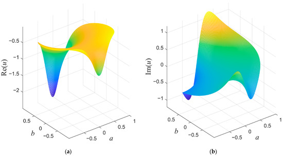
Figure 1. (a) Real part of u; (b) Imaginary part of $u$. Obtained at k = 1 and using “+” in corresponding equations.

3. Construction of the Hierarchy of Perturbed Korteweg–de Vries Equation

3.1. The perturbed Korteweg–de Vries Equation

In [14,15], the Lax Equation (1) is considered, where the operators $\widehat{M}$ and $\widehat{B}$ are matrices of the following form:

$$\widehat{M}=\left(\begin{array}{cc}\widehat{L}& \mu \widehat{N}\\ \widehat{N}& -\delta \widehat{L}\end{array}\right),\widehat{B}=\left(\begin{array}{cc}\widehat{A}& \mu \delta \widehat{R}\\ -\widehat{R}& \widehat{A}\end{array}\right),$$

(45)

where ${\delta }^2=1,$ $\mu$ is an arbitrary parameter; $\widehat{L}$, $\widehat{A}$ are the linear differential operators; $\widehat{N}$, $\widehat{R}$ are the scalar operators. With this approach, the Lax Equation (1) is equivalent to a system of two operator equations:

$${\widehat{L}}_t=\left[\widehat{L},\widehat{A}\right]-\mu \left(\widehat{N}\widehat{R}+\delta \widehat{R}\widehat{N}\right),$$

(46)

$${\widehat{N}}_t=\left[\widehat{N},\widehat{A}\right]+\widehat{R}\widehat{L}+\delta \widehat{L}\widehat{R}.$$

(47)

The operators $\widehat{L}$, $\widehat{A}$ have the same form as for the Korteweg–de Vries equation, i.e.,

$$\widehat{L}=-\frac{{\partial }^2}{\partial x^2}+u\left(x,t\right),\widehat{A}=4\frac{{\partial }^3}{\partial x^3}-3\left(u\frac{\partial }{\partial x}+\frac{\partial }{\partial x}u\right).$$

(48)

$\widehat{N}$ and $\widehat{R}$, respectively, have the values

$$\widehat{N}=w\left(x,t\right),\widehat{R}=b\left(x,t\right),$$

(49)

where $u\left(x,t\right)$, $w\left(x,t\right)$, $b\left(x,t\right)$ are the unknown functions.

From Equations (46) and (47) at $\delta =1,$ $b\left(x,t\right)=-6w_x$ one can obtain a system of equations:

$$\left\{\begin{array}{c}{u}_t=6u{u}_x-u_{xxx}+12\mu w{w}_x,\\ w_t=2w_{xxx}-6u{w}_x.\end{array}\right.$$

(50)

The resulting system can represent an example of the construction of the perturbed Korteweg–de Vries (KdV) equation

$$u_t+6u{u}_x+u_{xxx}=\epsilon f\left(u,u_x,\dots \right),0<\epsilon <1$$

(at $w\left(x,t\right)=0$ simply passing to KdV) with a special perturbation function $w\left(x,t\right)$, the dynamics of which are described by the second equation. Such a structure is satisfied by the first equation of system (50) at 0 < μ << 1, and the perturbation w(x,t) itself satisfies some law—the second equation of this system.

Several similar systems are considered in [10]. The first super-integrable KdV equation was proposed in [18,19] and has the following form:

$$\left\{\begin{array}{c}{u}_t=6u{u}_x-u_{xxx}-3\xi {\xi }_{xx},\\ {\xi }_t=-4{\xi }_{xxx}+3u_x\xi +6u{\xi }_x,\end{array}\right.$$

where u(x, t) is a bosonic function and ξ(x, t) is a fermionic function. It is bi-Hamiltonian and has an infinite number of conservation laws. Such systems are not unique; the following supersymmetric KdV system was proposed in [20]:

$$\left\{\begin{array}{c}{u}_t=6u{u}_x-u_{xxx}-3\xi {\xi }_{xx},\\ {\xi }_t=-4{\xi }_{xxx}+3{\left(u\xi \right)}_x,\end{array}\right.$$

which is a reduction of the supersymmetric Kadomtsev–Petviashvili hierarchy [21]. In [22], another new system, the superextension of the KdV hierarchy was constructed:

$$\left\{\begin{array}{c}{u}_t=6u{u}_x-u_{xxx}-12\xi {\xi }_{xx}+6u_x\xi {\xi }_x-3\xi {\xi }_{xxxx}-6{\xi }_x{\xi }_{xxx}, \\ {\xi }_t=-4{\xi }_{xxx}+3u_x\xi +6u{\xi }_x,\end{array}\right.$$

which is a super-integrable system describing a higher-order evolutionary perturbation.

Let us show that, as for the complex KdV expansion, there exists a hierarchy of perturbed systems associated with the higher KdV equations. For this purpose, we will use the existing operator system (46), (47), but replace the components of the operator $\widehat{B}$ with higher derivatives, preserving its skew-symmetry. Since the elements of the hierarchies are united by a common scattering operator, at the derivation the operator $\widehat{M}$ will retain the form specified in (45).

3.2. Hierarchy of the Perturbed Korteweg–de Vries Equation

Let us represent the operators (45) under the condition that $\delta =1,$ in the form:

$$\widehat{M}=\left(\begin{array}{cc}\widehat{L}& \mu \widehat{N}\\ \widehat{N}& -\widehat{L}\end{array}\right),{\widehat{B}}_j=\left(\begin{array}{cc}{\widehat{A}}_j& \mu {\widehat{R}}_j\\ -{\widehat{R}}_j& {\widehat{A}}_j\end{array}\right),j=1, 2, 3, \dots$$

(51)

Let us fix the operators $\widehat{L}$, $\widehat{N}$ in the form:

$$\widehat{L}=-\frac{{\partial }^2}{\partial x^2}+u\left(x,t\right),\widehat{N}=w\left(x,t\right).$$

(52)

Differential operators ${\widehat{A}}_j$ and ${\widehat{R}}_j$ have the following form:

$${\widehat{A}}_j={\alpha }_j\frac{{\partial }^{2j+1}}{\partial x^{2j+1}}+{\displaystyle \sum }_{m=1}^j\left(p_m\left(x,t\right)\frac{{\partial }^{2m-1}}{\partial x^{2m-1}}+\frac{{\partial }^{2m-1}}{\partial x^{2m-1}}{q}_m\left(x,t\right)\right),j=1, 2, 3, \dots$$

(53)

$${\widehat{R}}_j={\displaystyle \sum }_{m=0}^{2\left(j-1\right)}{b}_{2j-2-m}\left(x,t\right)\frac{{\partial }^{2j-2-m}}{\partial x^{2j-2-m}},$$

(54)

where $\mu$, ${\alpha }_j$ are arbitrary parameters, $p_m\left(x,t\right),q_m\left(x,t\right)$, $b_m\left(x,t\right)$ are unknown functions, the form of which will be clarified in the course of research.

The proof of the existence of a countable hierarchy of perturbed KdV equations will be carried out by the method of mathematical induction. Let us find out in which case the result of the new operators (53), (54) in the operator equations

$${\widehat{L}}_t=\left[\widehat{L},{\widehat{A}}_j\right]-\mu \left(\widehat{N}{\widehat{R}}_j+\delta {\widehat{R}}_j\widehat{N}\right),$$

(55)

$${\widehat{N}}_t=\left[\widehat{N},{\widehat{A}}_j\right]+{\widehat{R}}_j\widehat{L}+\delta \widehat{L}{\widehat{R}}_j$$

(56)

leads to a system of two partial differential equations for two unknown functions $u\left(x,t\right),w\left(x,t\right)$.

The proof of the first step of the method of mathematical induction for $j=1$ was carried out in [14,15]. Now we need to show that the solvability of the system (55) and (56) for $j=n+1$ with the operators ${\widehat{A}}_{n+1}$ and ${\widehat{R}}_{n+1}$ follows from the solvability of this system for $j=n$ with the operators ${\widehat{A}}_n$ and ${\widehat{R}}_n$ (the solvability of the system implies the reduction of the operator Equations (55) and (56) to two partial differential equations describing the dynamics of the functions $u\left(x,t\right)$ and $w\left(x,t\right)$, respectively).

Let us study in detail the structure of differential operators (53), (54). The operator ${\widehat{A}}_n$ contains two consecutive odd higher derivatives; compare ${\widehat{A}}_n$ and ${\widehat{A}}_{n+1}$:

$${\widehat{A}}_n={\alpha }_n\frac{{\partial }^{2n+1}}{\partial x^{2n+1}}+{\displaystyle \sum }_{m=1}^n\left(p_m\left(x,t\right)\frac{{\partial }^{2m-1}}{\partial x^{2m-1}}+\frac{{\partial }^{2m-1}}{\partial x^{2m-1}}{q}_m\left(x,t\right)\right)={\alpha }_n\frac{{\partial }^{2n+1}}{\partial x^{2n+1}}+D_{2n-1},$$

(57)

$${\widehat{A}}_{n+1}={\alpha }_{n+1}\frac{{\partial }^{2n+3}}{\partial x^{2n+3}}+p_{n+1}\frac{{\partial }^{2n+1}}{\partial x^{2n+1}}+\frac{{\partial }^{2n+1}}{\partial x^{2n+1}}{q}_{n+1}+D_{2n-1},$$

(58)

where $D_{2n-1}$ is the differential terms from $2n-1$ order and below.

As can be seen for ${\widehat{A}}_{n+1}$, increasing the index n by one increases the degree of the derivative by two orders of magnitude, adding two new unknown functions $p_{n+1}\left(x,t\right),q_{n+1}\left(x,t\right)$, which will be predetermined by transformations of the operator Equations (55) and (56).

Similarly, let us analyze for ${\widehat{R}}_n$. ${\widehat{R}}_n$ has a senior even derivative; when the index n increases by one ${\widehat{R}}_{n+1}$, the degree of the differential terms increases by two orders of magnitude, so let us represent the two consecutive operators in the form:

$${\widehat{R}}_n={\displaystyle \sum }_{m=0}^{2n-2}{b}_{2n-2-m}\left(x,t\right)\frac{{\partial }^{2n-2-m}}{\partial x^{2n-2-m}},\hspace{1em}{\widehat{R}}_{n+1}=b_{2n}\left(x,t\right)\frac{{\partial }^{2n}}{\partial x^{2n}}+b_{2n-1}\left(x,t\right)\frac{{\partial }^{2n-1}}{\partial x^{2n-1}}+{\widehat{R}}_n.$$

(59)

As the order of the linear differential operator increases, the number of unknown functions also increases, and two new functions $b_{2n}\left(x,t\right),b_{2n-1}\left(x,t\right)$ arise that can also be further predetermined.

Let us show that as the order of the differential operators of the given form (58), (59) increases, the resulting systems for the unknown coefficients $p_m\left(x,t\right),q_m\left(x,t\right),b_m\left(x,t\right)$, $m=0,1,\dots ,2n-2$ do not become overdetermined.

For this, we write the system (55), (56) for for j = n:

$$u_t=\left[\widehat{L},D_{2n-1}\right]+{\alpha }_{n}u\frac{{\partial }^{2n+1}}{\partial x^{2n+1}}-{\alpha }_n{\displaystyle \sum }_{j=0}^{2n+1}{C}_{2n+1}^j{u}_{x^j}\frac{{\partial }^{2n+1-j}}{\partial x^{2n+1-j}}-\mu \left(w{\widehat{R}}_n+{\widehat{R}}_{n}w\right),$$

(60)

$$w_t={\alpha }_{n}w\frac{{\partial }^{2n+1}}{\partial x^{2n+1}}-{\alpha }_n{\displaystyle \sum }_{j=0}^{2n+1}{C}_{2n+1}^j{w}_{x^j}\frac{{\partial }^{2n+1-j}}{\partial x^{2n+1-j}}+\left[w,D_{2n-1}\right]+{\widehat{R}}_n\widehat{L}+\widehat{L}{\widehat{R}}_n.$$

(61)

Let us group the elements with differential operators of the same order and equate these coefficients to zero:

$$\frac{{\partial }^{2n}}{\partial x^{2n}}:\left\{\begin{array}{c}-{\alpha }_n\left(2n+1\right)u_x-2p_{nx}-2q_{nx}=0,\\ -{\alpha }_n\left(2n+1\right)w_x-2b_{2n-2}=0,\end{array}\right.$$

(62)

$$\frac{{\partial }^{2n-1}}{\partial x^{2n-1}}:\left\{\begin{array}{c}\left(4n-1\right)q_{nxx}+p_{nxx}+\left(2n+1\right)n{\alpha }_n{u}_{xx}=0,\\ {\alpha }_n\left(2n+1\right)n{w}_{xx}+2b_{2n-3}+2b_{\left(2n-2\right)x}=0,\end{array}\right.$$

(63)

…

$$1:\left\{\begin{array}{c}{u}_t={\displaystyle \sum _{j=1}^n}[u{q}_{j{x}^{2j-1}}-q_{j{x}^{2j+1}}-p_j{u}_{x^{2j-1}}-\left(q_{j}u{)}_{x^{2j-1}}\right]-{\alpha }_n{u}_{x^{2n+1}}-\mu \left[w{b}_0+{\displaystyle \sum _{j=0}^{2n-2}}{b}_j{w}_{x^j}\right],\\ w_t=-{\alpha }_n{w}_{x^{2n+1}}+{\displaystyle \sum _{j=1}^n}[w{q}_{j{x}^{2j-1}}-p_j{w}_{x^{2j-1}}-\left(q_{j}w{)}_{x^{2j-1}}\right]+{\displaystyle \sum _{j=0}^{2n-2}}{b}_j{u}_{x^j}-b_{0xx}+u{b}_0.\end{array}\right.$$

(64)

Non-trivial equations are obtained, from which the previously unknown functions are redefined $p_m\left(x,t\right),q_m\left(x,t\right),b_m\left(x,t\right)$:

$$b_{2n-2}=-\frac{{\alpha }_n}{2}\left(2n+1\right)w_x,b_{2n-3}=\frac{{\alpha }_n}{2}\left(2n+1\right)\left(1-n\right)w_{xx},p_n=q_n=-\frac{{\alpha }_n}{4}\left(2n+1\right)u.$$

The last pair of (64) gives the desired system on functions $u\left(x,t\right)$ and $w\left(x,t\right)$.

Now let us perform a similar action for $j=n+1$ and make a grouping of coefficients at differential operators:

$$\frac{{\partial }^{2n+2}}{\partial x^{2n+2}}:\left\{\begin{array}{c}-{\alpha }_{n+1}\left(2n+3\right)u_x-2p_{\left(n+1\right)x}-2q_{\left(n+1\right)x}=0,\\ -{\alpha }_{n+1}\left(2n+3\right)w_x-2b_{2n}=0,\end{array}\right.$$

(65)

$$\frac{{\partial }^{2n+1}}{\partial x^{2n+1}}:\left\{\begin{array}{c}\left(4n+3\right)q_{\left(n+1\right)xx}+p_{\left(n+1\right)xx}+\left(2n+3\right)\left(n+1\right){\alpha }_{n+1}{u}_{xx}=0,\\ {\alpha }_{n+1}\left(2n+3\right)\left(n+1\right)w_{xx}+2b_{2n-1}+2b_{2nx}=0,\end{array}\right.$$

(66)

…

$$1:\left\{\begin{array}{c}{u}_t={\displaystyle \sum _{j=1}^{n+1}}[u{q}_{j{x}^{2j-1}}-q_{j{x}^{2j+1}}-p_j{u}_{x^{2j-1}}-\left(q_{j}u{)}_{x^{2j-1}}\right]-{\alpha }_{n+1}{u}_{x^{2n+3}}-\mu \left[w{b}_0+{\displaystyle \sum _{j=0}^{2n}}{b}_j{w}_{x^j}\right],\\ w_t=-{\alpha }_{n+1}{w}_{x^{2n+3}}+{\displaystyle \sum _{j=1}^{n+1}}[w{q}_{j{x}^{2j-1}}-p_j{w}_{x^{2j-1}}-\left(q_{j}w{)}_{x^{2j-1}}\right]+{\displaystyle \sum _{j=0}^{2n}}{b}_j{u}_{x^j}-b_{0xx}+u{b}_0\end{array}\right..$$

(67)

Comparing the differential operators obtained at $j=n$ and $j=n+1$, we see that only two non-trivial systems are added, corresponding to $\frac{{\partial }^{2n+2}}{\partial x^{2n+2}}$, $\frac{{\partial }^{2n+1}}{\partial x^{2n+1}}$. We have a total of four equations from which the functions are uniquely defined:

$$\begin{array}{c}{p}_{n+1}\left(x,t\right)=q_{n+1}\left(x,t\right)=-\frac{{\alpha }_{n+1}}{2}\left(2n+3\right)u,\\ b_{2n}\left(x,t\right)=-\frac{{\alpha }_{n+1}}{2}\left(2n+3\right)w_x, b_{2n-1}\left(x,t\right)=-\frac{{\alpha }_{n+1}}{2}n\left(2n+3\right)w_{xx}.\end{array}$$

(68)

The number of remaining differential operators from $\frac{{\partial }^{2n}}{\partial x^{2n}}$ and below coincides with their number for $j=n$ and corresponds to the number of unknown functions $p_m\left(x,t\right),q_m\left(x,t\right),b_m\left(x,t\right)$ (by conjecture); hence, the overdetermination of the system does not arise. As a result, the following theorem is proved.

Theorem 2.

The system (55), (56) with operators of the form (52)–(54) generates a hierarchy of the perturbed Korteweg–de Vries equation on functions $u\left(x,t\right)$ and $w\left(x,t\right)$ of the form (64), where all functions $p_j\left(x,t\right),q_j\left(x,t\right),b_j\left(x,t\right),j=1, 2, \dots , n$, being coefficients of operators ${\widehat{A}}_n, {\widehat{R}}_n$, are defined uniquely from system (62), (63); and $\mu$ is an arbitrary parameter.

Analyzing the structure of obtained systems at higher derivatives (60)–(63), one can notice that the first equations in pairs define the dependence of operator ${\widehat{A}}_n$ coefficients $p_m\left(x,t\right),q_m\left(x,t\right)$ on function $u\left(x,t\right)$ and its derivatives, and the second equations in pairs define operator ${\widehat{R}}_n$ coefficients $b_m\left(x,t\right)$ via function $w\left(x,t\right)$ and its derivatives (68). Assuming that there is no perturbation $w\left(x,t\right)=0$, the operators (51) $\widehat{M}$ and ${\widehat{B}}_n$ are transformed into operators $\widehat{L},$and ${\widehat{A}}_n$ ($\widehat{N}=0$, ${\widehat{R}}_n=0$), which are Lax pairs for the KdV hierarchy equations. Consequently, all systems (64) will be transformed to higher KdV hierarchy equations.

In addition, from system (64) we can now obtain at once all the equations of the KdV hierarchy expressed through the operator ${\widehat{A}}_n$ coefficients:

$$u_t={\displaystyle \sum _{j=1}^n}[u{q}_{j{x}^{2j-1}}-q_{j{x}^{2j+1}}-p_j{u}_{x^{2j-1}}-\left(q_{j}u{)}_{x^{2j-1}}\right]-{\alpha }_n{u}_{x^{2n+1}}.$$

(69)

Theorem 3.

If the functions $u\left(x,t\right)$ and $w\left(x,t\right)$ satisfy the system (64), then the invariant transformations exist for solutions of the eigenvalue equation $\left(\widehat{M}-\lambda E\right)V=0$ with operator $\widehat{M}$ (45) of the form 

$${\widehat{H}}_n=\left(\begin{array}{cc}{\widehat{A}}_n& \mu {\widehat{R}}_n\\ -{\widehat{R}}_n& {\widehat{A}}_n\end{array}\right)-\left(\begin{array}{cc}1& 0\\ 0& 1\end{array}\right)\frac{\partial }{\partial t},n=1,2,3,\dots$$

(70)

where $V=\left(\begin{array}{c}{v}_1\left(\lambda ,x,t\right)\\ v_2\left(\lambda ,x,t\right)\end{array}\right)$ is the vector-function, ${\widehat{A}}_j$, ${\widehat{R}}_j$ have the form (53), (54), $\lambda , \mu$ are the arbitrary parameters.

Proof of Theorem 3.

Consider the action of operators $\widehat{M}$ and ${\widehat{H}}_n$ on the vector-function $V=\left(\begin{array}{c}{v}_1\left(\lambda ,x,t\right)\\ v_2\left(\lambda ,x,t\right)\end{array}\right)$:

$$\left(\begin{array}{cc}\widehat{L}-\lambda & \mu \widehat{N}\\ \widehat{N}& -\widehat{L}-\lambda \end{array}\right)\left[\left(\begin{array}{cc}{\widehat{A}}_1& \mu {\widehat{R}}_1\\ -{\widehat{R}}_1& {\widehat{A}}_1\end{array}\right)+\frac{\partial }{\partial t}\right]\left(\begin{array}{c}{v}_1\\ v_2\end{array}\right)=\left(\begin{array}{c}\left(\widehat{L}{\widehat{A}}_1-\lambda {\widehat{A}}_1-\mu \widehat{N}{\widehat{R}}_1\right)v_1+\mu \left(\widehat{L}{\widehat{R}}_1-\lambda {\widehat{R}}_1+\widehat{N}{\widehat{A}}_1\right)v_2+\left(\widehat{L}-\lambda \right)v_{1t}+\mu \widehat{N}{v}_{2t}\\ \left(\widehat{N}{\widehat{A}}_1+\widehat{L}{\widehat{R}}_1+\lambda {\widehat{R}}_1\right)v_1+\left(\mu \widehat{N}{\widehat{R}}_1-\widehat{L}{\widehat{A}}_1-\lambda {\widehat{A}}_1\right)v_2-\left(\widehat{L}+\lambda \right)v_{2t}+\widehat{N}{v}_{1t}\end{array}\right).$$

(71)

Since the functions $v_1, v_2$ are solutions of a homogeneous equation

$$\left(\begin{array}{cc}\widehat{L}& \mu \widehat{N}\\ \widehat{N}& -\widehat{L}\end{array}\right)\left(\begin{array}{c}{v}_1\\ v_2\end{array}\right)-\lambda \left(\begin{array}{cc}1& 0\\ 0& 1\end{array}\right)\left(\begin{array}{c}{v}_1\\ v_2\end{array}\right)=0,$$

the following equations take place

$$\widehat{L}{v}_1+\mu \widehat{N}{v}_2=\lambda v_1,\widehat{N}{v}_1-\widehat{L}{v}_2=\lambda v_2.$$

(72)

Let us differentiate (72) by t, and determine the result of the operator $\widehat{M}-\lambda E$ action on the functions $v_{1t}\left(\lambda ,x,t\right),v_{2t}\left(\lambda ,x,t\right)$:

$$\begin{array}{c}{v}_{1xxt}=u_t{v}_1+\mu w_t{v}_2+u{v}_{1t}+\mu w{v}_{2t}-\lambda v_{1t},\\ v_{2xxt}=u_t{v}_2+u{v}_{2t}+\lambda v_{2t}-w_t{v}_1-w{v}_{1t},\end{array}$$

or in operator form

$$\left(\begin{array}{cc}\widehat{L}-\lambda & \mu \widehat{N}\\ \widehat{N}& -\widehat{L}-\lambda \end{array}\right)\left(\begin{array}{c}{v}_{1t}\\ v_{2t}\end{array}\right)=-\left(\begin{array}{cc}{u}_t& \mu w_t\\ w_t& -u_t\end{array}\right)\left(\begin{array}{c}{v}_1\\ v_2\end{array}\right)=-\left(\begin{array}{cc}{\widehat{L}}_t& \mu {\widehat{N}}_t\\ {\widehat{N}}_t& -{\widehat{L}}_t\end{array}\right)\left(\begin{array}{c}{v}_1\\ v_2\end{array}\right).$$

(73)

Then, using (72), (73) in (71) we can get rid of the parameter $\lambda$ and the derivatives $v_{1t}\left(\lambda ,x,t\right),v_{2t}\left(\lambda ,x,t\right)$.

The equation $\left(\widehat{M}-\lambda E\right){\widehat{H}}_{n}V=0$ will take the form of a system

$$\begin{array}{c}\widehat{(L}{\widehat{A}}_n-\mu \widehat{N}{\widehat{R}}_n-{\widehat{L}}_t)v_1-{\widehat{A}}_n\left(\widehat{L}{v}_1+\mu \widehat{N}{v}_2\right)+\mu \left(\widehat{L}{\widehat{R}}_n+\widehat{N}{\widehat{A}}_n-{\widehat{N}}_t\right)v_2-\mu {\widehat{R}}_n\left(\widehat{N}{v}_1-\widehat{L}{v}_2\right)=0,\\ \left(\widehat{N}{\widehat{A}}_n+\widehat{L}{\widehat{R}}_n-{\widehat{N}}_t\right)v_1+{\widehat{R}}_n\left(\widehat{L}{v}_1+\mu \widehat{N}{v}_2\right)+\left(\mu \widehat{N}{\widehat{R}}_n-\widehat{L}{\widehat{A}}_n+{\widehat{L}}_t\right)v_2-{\widehat{A}}_n\left(\widehat{N}{v}_1-\widehat{L}{v}_2\right)=0.\end{array}$$

Let us group the terms with $v_1,v_2$:

$$\begin{array}{c}\left(\left[\widehat{L},{\widehat{A}}_n\right]-\mu \widehat{N}{\widehat{R}}_n-{\widehat{L}}_t-\mu {\widehat{R}}_n\widehat{N}\right)v_1+\mu \left(\widehat{L}{\widehat{R}}_n+{\widehat{R}}_n\widehat{L}+\left[\widehat{N},{\widehat{A}}_n\right]-{\widehat{N}}_t\right)v_2=0,\\ \left(\left[\widehat{N},{\widehat{A}}_n\right]+\widehat{L}{\widehat{R}}_n-{\widehat{N}}_t+{\widehat{R}}_n\widehat{L}\right)v_1+\left(\mu \widehat{N}{\widehat{R}}_n-\left[\widehat{L},{\widehat{A}}_n\right]+{\widehat{L}}_t+\mu {\widehat{R}}_n\widehat{N}\right)v_2=0.\end{array}$$

(74)

It is easy to see that in (74) the coefficients at $v_1, v_2$ are operators of structures (55), (56) at $\delta =1$, which reduce to the system (64), which proves the theorem. □

3.3. Perturbation of the Second Korteweg–de Vries Hierarchy

Let us construct an explicit form of the system describing the perturbation of the second KdV equation. Let us write the elements of operators ${\widehat{B}}_2$, ${\widehat{R}}_2$, and ${\widehat{A}}_2$ in the form (53), (54), and the remaining elements (51), (52) retain the same form

$${\widehat{R}}_2=b_2\left(x,t\right)\frac{{\partial }^2}{\partial x^2}+b_1\left(x,t\right)\frac{\partial }{\partial x}+b_0\left(x,t\right),$$

(75)

$${\widehat{A}}_2={\alpha }_2\frac{{\partial }^5}{\partial x^5}+p_2\frac{{\partial }^3}{\partial x^3}+\frac{{\partial }^3}{\partial x^3}{q}_2+p_1\frac{\partial }{\partial x}+\frac{\partial }{\partial x}{q}_1,$$

(76)

where $b_i\left(x,t\right),i=0,1,2$, $p_j\left(x,t\right),q_j\left(x,t\right),j=1, 2$ are unknown functions, the form of which we will specify later, ${\alpha }_2$ is an arbitrary constant.

Let us define the form of the system (55), (56). Let us expand the differentiation operators (55) and equate the coefficients at $\frac{{\partial }^4}{\partial x^4}$, $\frac{{\partial }^3}{\partial x^3}$, $\frac{{\partial }^2}{\partial x^2}$, $\frac{\partial }{\partial x}$ to zero; then, we obtain the system:

$$\begin{array}{c}\frac{{\partial }^4}{\partial x^4}: 2q_{2x}+2p_{2x}+5{\alpha }_2{u}_x=0,\\ \frac{{\partial }^3}{\partial x^3}: 10{\alpha }_2{u}_{xx}+p_{2xx}+7q_{2xx}=0,\\ \frac{{\partial }^2}{\partial x^2}: 9q_{2xxx}+10{\alpha }_2{u}_{xxx}+2p_{1x}+2q_{1x}+3p_2{u}_x+3q_2{u}_x+\mu b_{2}w\left(1+\delta \right)=0,\\ \frac{\partial }{\partial x}: 5q_{2x^4}+3q_{1xx}-3u{q}_{2xx}+3{\left(q_{2}u\right)}_{xx}+p_{1xx}+3p_2{u}_{xx}+\mu \left(\delta +1\right)b_{1}w\\ +2\mu \delta b_2{w}_x+5{\alpha }_2{u}_{x^4}=0,\\ 1: u_t\left(x,t\right)=u{q}_{1x}-q_{2x^5}-q_{1xxx}+u{q}_{2xxx}-{\alpha }_2{u}_{x^5}-p_2{u}_{xxx}-{\left(q_{2}u\right)}_{xxx}\\ -p_1{u}_x-{\left(q_{1}u\right)}_x-\mu b_{0}w\left(1+\delta \right)-\mu \delta b_2{w}_{xx}-\mu \delta b_1{w}_x.\end{array}$$

(77)

From the first four equations of the system (77) the following functions are defined (the integration constants are assumed to be equal to zero):

$$q_2=p_2=-\frac{5}{4}{\alpha }_{2}u, p_{1x}=\frac{5}{8}{\alpha }_2{u}_{xxx}+\frac{15}{4}{\alpha }_{2}u{u}_x-\frac{\mu \left(1+\delta \right)}{2}{b}_{2}w-q_{1x},$$

(78)

$$q_{1xx}=\frac{5}{16}{\alpha }_2{u}_{xxxx}+\frac{15}{16}{\alpha }_2{u}_{xx}^2+\frac{\mu \left(1+\delta \right)}{4}{(b_{2}w)}_x-\frac{\mu \left(1+\delta \right)}{2}{b}_{1}w-\mu \delta b_2{w}_x.$$

(79)

Let us perform a similar procedure with the operator equation (56), resulting in the following system:

$$\begin{array}{l}\frac{{\partial }^4}{\partial x^4}: 5{\alpha }_2{w}_x+\left(1+\delta \right)b_2=0,\\ \frac{{\partial }^3}{\partial x^3}:10{\alpha }_2{w}_{xx}+\left(1+\delta \right)b_1+2\delta b_{2x}=0,\\ \frac{{\partial }^2}{\partial x^2}: 3w{q}_{2x}+\left(1+\delta \right)\left(u{b}_2-b_0\right)-10{\alpha }_2{w}_{xxx}-3p_2{w}_x-3{\left(q_{2}w\right)}_x-\delta b_2{}_{xx}-2\delta b_1{}_x=0,\\ \frac{\partial }{\partial x}: 3w{q}_{2xx}-5{\alpha }_2{w}_{x^4}+2b_2{u}_x+\left(1+\delta \right)b_{1}u-3p_2{w}_{xx}-3{\left(q_{2}w\right)}_{xx}-\delta b_1{}_{xx}-2\delta b_0{}_x=0,\\ 1: w_t=w{q}_{2xxx}-{\alpha }_2{w}_{x^5}-\delta b_0{}_{xx}+b_2{u}_{xx}+b_1{u}_x+b_{0}u-p_2{w}_{xxx}+\delta u{b}_0-{\left(q_{2}w\right)}_{xxx}\\ -p_1{w}_x-q_1{w}_x.\end{array}$$

(80)

The values of the functions are uniquely defined:

$$b_2\left(x,t\right)=-5\frac{{\alpha }_2}{\delta +1}{w}_x,b_1\left(x,t\right)=-\frac{10{\alpha }_2}{{(\delta +1)}^2}{w}_{xx},$$

(81)

$$b_0\left(x,t\right)=\frac{5{\alpha }_2}{2\left(1+\delta \right)}u{w}_x+5{\alpha }_2\frac{4\delta -\left(\delta +1\right)\left(\delta +2\right)}{{(\delta +1)}^3}{w}_{xxx},$$

(82)

$$5{\alpha }_2\left(2\delta \frac{{\delta }^2+3}{{(\delta +1)}^3}-1\right)w_{x^4}+\frac{5{\alpha }_2}{\delta +1}\frac{1}{2}\left(\delta -1\right)\left(u_x{w}_x+u{w}_{xx}\right)=0.$$

(83)

For (83) to be true identically, it is necessary to put the coefficients equal to zero:

$$2\delta \frac{{\delta }^2+3}{{(\delta +1)}^3}-1=0, \delta -1=0.$$

It is possible at $\delta =1$.

As a result, from the two systems (77), (80) only the last equations that form the dynamical system remain. Let us substitute the found values of the functions by putting ${\alpha }_2=-16$, and we obtain the system:

$$\begin{array}{c}{u}_t={[u_{xxxx}-10u{u}_{xx}-5u_x^2+10u^3-20\mu \left(w_{xx}w-w^{2}u\right)]}_x,\\ w_t=-4w_{x^5}+20u{w}_{xxx}+20w_{xx}{u}_x+10w_x{u}_{xx}+10\left(2\mu w^2-u^2\right)w_x.\end{array}$$

(84)

As a result of this reasoning, the following corollary is proven.

Corollary 8.

The nonlinear system of Equation (84) has the operator representation (55), (56) with operators of the form (52), where $\widehat{L}$ is the Sturm–Liouville operator, and the other operators have the form 

$${\widehat{R}}_2=40\left(w_x\frac{{\partial }^2}{\partial x^2}+w_{xx}\frac{\partial }{\partial x}+\frac{1}{2}\left[u{w}_x-w_{xxx}\right]\right),\widehat{N}=w\left(x,t\right),$$

(85)

$${\widehat{A}}_2=-16\frac{{\partial }^5}{\partial x^5}+20u\frac{{\partial }^3}{\partial x^3}+20\frac{{\partial }^3}{\partial x^3}u-5\left(u_{xx}+3u^2+2\mu w^2\right)\frac{\partial }{\partial x}-5\frac{\partial }{\partial x}\left(u_{xx}+3u^2+2\mu w^2\right),$$

(86)

 where  $\delta =1$,  $u\left(x,t\right),w\left(x,t\right)$  are arbitrary real functions,  $\mu$  is an arbitrary parameter.

The system (84) is a perturbation of the second equation of the KdV hierarchy, since when $w=0$ and at replacement $u\left(x,t\right)\to -u\left(x,t\right)$ the system is reduced to one equation, and this is the second equation of the KdV hierarchy:

$$u_t={(u_{xxxx}+5u_x^2+10u{u}_{xx}+10u^3)}_x.$$

In the particular case when $\mu =1$, and the functions $u\left(x,t\right)$, $w\left(x,t\right)$ represent, respectively, the real and imaginary parts of some complex function $q\left(x,t\right)=u\left(x,t\right)+iw\left(x,t\right)$, the system (84) describes the behavior of the real and imaginary parts of the second equation of the KdV complexification hierarchy:

$$\begin{array}{c}{q}_t=10\left(q^2+{\left|q\right|}^2\right){\stackrel{-}{q}}_x+\frac{5}{2}\left({\stackrel{-}{q}}^2+6{\left|q\right|}^2-3q^2\right)q_x-5q_x{(\stackrel{-}{q}+3q)}_{xx}-10q{\stackrel{-}{q}}_{xxx}\\ -\frac{5}{4}{\left(2{\left|q\right|}^2-3q^2+3{\stackrel{-}{q}}^2\right)}_{\mathit{xxx}}+\frac{1}{2}{(5\stackrel{-}{q}-3q)}_{xxxxx}\end{array}$$

4. Conclusions

In this paper we use the Lax operator equation, where the scattering operator is a Hermitian differential operator of the fourth order and the operator determining the dynamics of the eigenfunctions is a skew-symmetric differential operator with an odd higher order. We consider the possibility of constructing a hierarchy of the complex extension of the Korteweg–de Vries equation and a hierarchy of its perturbation with a special perturbation function. The first and second parts are based on the Lax method with operators having a matrix structure.

It is proved that for the equation on the eigenvalues of the fourth-order scattering operator, there exists a countable number of ${\widehat{H}}_n$ operators that translate its solution into its other solution. Moreover, ${\widehat{H}}_n$ operators are considered as differential operators of order 2n + 1, which generate a hierarchy of cKdV and a hierarchy of pKdV.

All obtained equations describe nonlinear waves arising in various media with dispersion, and mainly these are problems of gas and hydrodynamics.

The obtained new nonlinear equations and systems possess a Lax pair, and hence one can expect the following properties: an infinite number of conservation laws, Painlevé coupling of the partial differential equation with the system of ordinary differential equations, Hamiltonian structure, Hirota formalism for constructing n-soliton solutions, Bäcklund transformations, etc.

References

- Gardner, C.S.; Greene, J.M.; Kruskal, M.D.; Miura, R.M. Method for solving the Korteweg-de Vries equation. Phys. Rev. Lett. 1967, 19, 1095–1097. [Google Scholar] [CrossRef]
- Liu, X.-K.; Wen, X.-Y. A discrete KdV equation hierarchy: Continuous limit, diverse exact solutions and their asymptotic state analysis. Commun. Theor. Phys. 2022, 74, 065001. [Google Scholar] [CrossRef]
- Li, F.; Yao, Y. Multisoliton and rational solutions for the extended fifth-order KdV equation in fluids with self-consistent sources. Theor. Math. Phys. 2022, 210, 184–197. [Google Scholar] [CrossRef]
- Zemlyanukhin, A.I.; Bochkarev, A.V. The perturbation method and exact solutions of nonlinear dynamics equations for media with microstructure. Comput. Contin. Mech. 2016, 9, 182–191. [Google Scholar] [CrossRef]
- Kudryashov, N.A. Remarks on rational solutions for the Korteweg-de Vries hierarchy. arXiv 2007, arXiv:nlin/0701034. [Google Scholar]
- Clarkson, P.A.; Joshi, N.; Mazzocco, M. The Lax pair for the mKdV hierarchy. Sémin. Congrès 2006, 14, 53–64. [Google Scholar]
- Ye, S.; Zeng, Y. Integration of the modified Korteweg-de Vries hierarchy with an integral type of source. J. Phys. A Math. Gen. 2002, 35, L283–L291. [Google Scholar] [CrossRef]
- Joshi, N. The second Painlevé hierarchy and the stationary KdV hierarchy. Publ. Res. Inst. Math. Sci. 2004, 40, 1039–1061. [Google Scholar] [CrossRef]
- Zabrodin, A.V. Kadomtsev–Petviashvili hierarchies of types B and C. Theor. Math. Phys. 2021, 208, 865–885. [Google Scholar] [CrossRef]
- Zhang, Y.; Rui, W. A few super-integrable hierarchies and some re-ductions, super-Hamiltonian structures. Rep. Math. Phys. 2015, 75, 231–255. [Google Scholar] [CrossRef]
- Liu, J.-G.; Yang, X.-J.; Feng, Y.-Y.; Cui, P.; Geng, L.-L. On integrability of the higher dimensional time fractional KdV-type equation. J. Geom. Phys. 2021, 160, 104000. [Google Scholar] [CrossRef]
- Kundu, A. Integrable twofold hierarchy of perturbed equations and application to optical soliton dynamics. Theor. Math. Phys. 2011, 167, 800–810. [Google Scholar] [CrossRef]
- Redkina, T.V.; Zakinyan, R.G.; Zakinyan, A.R.; Surneva, O.B.; Yanovskaya, O.S. Bäcklund Transformations for Nonlinear Differential Equations and Systems. Axioms 2019, 8, 45. [Google Scholar] [CrossRef]
- Bogoyavlenskiĭ, O.I. Breaking solitons II. Math. USSR Izv. 1990, 35, 245–248. [Google Scholar] [CrossRef]
- Bogoyavlenskiĭ, O.I. Breaking solitons III. Math. USSR Izv. 1991, 36, 129–137. [Google Scholar] [CrossRef]
- Redkina, T.V. Some properties of the complexification of the Korteweg-de Vries equation. Izv. Acad. Sci. USSR Ser. Math. 1991, 55, 1300–1311. [Google Scholar]
- Lax, P.D. Integrals of nonlinear equation of evolution and solitary waves. Commun. Pure Appl. Math. 1968, 21, 467–490. [Google Scholar] [CrossRef]
- Kuperschmidt, B.A. Integrable and Super-Integrable Systems; World Scientific: Singapore, 1990. [Google Scholar]
- Kuperschmidt, B.A. A super Korteweg-de Vries equation: An integrable system. Phys. Lett. A 1984, 102, 213–215. [Google Scholar] [CrossRef]
- Manin, Y.I.; Radul, A.O. A supersymmetric extension of the Kadomtsev-Petviashvili hierarchy. Commun. Math. Phys. 1985, 98, 65–77. [Google Scholar] [CrossRef]
- Magnot, J.P.; Rubtsov, V.N. On the Kadomtsev-Petviashvili hierarchy in an extended class of formal pseudo-differential operators. Theor. Math. Phys. 2021, 207, 458–488. [Google Scholar] [CrossRef]
- Geng, X.; Wu, L. A new super-extension of the KdV hierarchy. Appl. Math. Lett. 2010, 23, 716–721. [Google Scholar] [CrossRef]
Disclaimer/Publisher’s Note: The statements, opinions and data contained in all publications are solely those of the individual author(s) and contributor(s) and not of MDPI and/or the editor(s). MDPI and/or the editor(s) disclaim responsibility for any injury to people or property resulting from any ideas, methods, instructions or products referred to in the content. |
© 2023 by the authors. Licensee MDPI, Basel, Switzerland. This article is an open access article distributed under the terms and conditions of the Creative Commons Attribution (CC BY) license (https://creativecommons.org/licenses/by/4.0/).