Kinematic Differential Geometry of a Line Trajectory in Spatial Movement

Abstract

This paper investigates the kinematic differential geometry of a line trajectory in spatial movement. Specifically, we provide a theoretical expression of inflection line congruence, which is the spatial equivalent of the inflection circle of planar kinematics. Additionally, we introduce new proofs for the Euler–Savary and Disteli formulae and thoroughly analyze their spatial equivalence.

1. Introduction

The study of the kinematic differential geometry of a line trajectory in spatial movement is of considerable significance in various areas, including mathematics, physics, and engineering. Under the conditions of spatial movements, invariants give valuable information about the behavior of objects as they travel through space. One of the prime reasons for researching a line trajectory is to understand the geometric and kinematic properties of moving objects. Differential geometry can be used to describe the trajectory, velocity, and acceleration of a line as it moves through space, providing insights into its physical behavior. Moreover, it can be used to construct mathematical models of moving lines, which can be used to design and optimize complex engineering systems. Kinematic differential geometry can be used to characterize the geometry of ruled surfaces, such as their curvature and torsion. This relationship between kinematic properties and ruled surfaces has important applications in fields such as computer graphics and architecture, for example [1,2,3,4,5,6,7]. Throughout the spatial movement of two rigid bodies, the instantaneous screw axis ($\mathbb{ISA}$) changes its attitude and possessions and creates two distinct but coupled ruled surfaces: the stationary axode in the stationary body and the moveable axode in the moveable body. Throughout the movement, the axodes slide and roll with respect to each other in a certain way such that tangential touch between the axodes is permanently conserved by the full length of the two mating rulings (one being in each axode), which together display the $\mathbb{ISA}$ at all instants. It is significant that not only does a specific movement yield altitude to a unique family of axodes but that the converse also applies. This shows that, should the axodes of any movement be known, the given movement can be re-established without seeking the physical components of the mechanism, their community, specific dimensions, or the strategy by which they are established [1,2,3,7,8,9].

One of the ultimate appropriate ways to research a line trajectory in spatial movement appears to realize an interrelation between this space and dual numbers. Dual numbers were first proposed by W. Clifford and after, they and E. Study used them as an instrument for their research on differential line geometry and kinematics. They gave specific attention to the exemplification of directed lines by dual unit vectors and realized the mapping that is known by their name. The E. Study map states that:

The oriented lines in the Euclidean 3-space ${\mathbb{E}}^3$ are in one-to-one correspondence with the points on the dual unit sphere in the dual 3-space ${\mathbb{D}}^3$ [1,2,3]. It authorizes a perfect expansion of mathematical statement into spherical point geometry into spatial line geometry through dual numbers expansion, that is, replacing all ordinary quantities by the congruent dual numbers quantities. There exists a significant body of work on E. Study maps, including various monographs [10,11,12,13,14,15,16,17,18].

In this work, based on the E. Study map, the kinematic differential geometry of a line trajectory in spatial movement is investigated. The classical results of spatial kinematics are obtained in this way, as well as new loci of lines which instantaneously create special trajectories. The inflection line congruence is determined and discussed in detail, and the invariants of the axodes are utilized for establishing a new proof of Disteli’s formulae. Our findings contribute to a deeper understanding of the interplay between spatial movements and axodes, with potential applications in fields such as robotics and mechanical engineering.

2. Preliminaries

In this section, we present some notations of dual numbers and dual vectors (see [1,2,3,10,11,12,13,14,15,16,17,18]). A dual number $\widehat{\alpha }$ has the form $\widehat{\alpha }=\alpha +\epsilon {\alpha }^{*}$, where $\alpha$ and ${\alpha }^{*}$ are real numbers. Here, $\epsilon$ is a dual unit subject to $\epsilon \ne 0,{\epsilon }^2=0,\epsilon .1=1.\epsilon =\epsilon .$ The set of dual numbers, $\mathbb{D}$, forms a commutative ring containing the numbers $\epsilon {\alpha }^{*}$ (${\alpha }^{*}$ is real) as divisors of zero. $\mathbb{D}$ is not a field. No number $\epsilon {\alpha }^{*}$ has an inverse. However, the other laws of the algebra of dual numbers are the same as those of complex numbers [1,2,3,4,5,6].

For all pairs $(\alpha ,{\alpha }^{*})\in {\mathbb{E}}^3\times {\mathbb{E}}^3$ the set

$${\mathbb{D}}^3=\{\widehat{\mathsf{\alpha }}:=\mathsf{\alpha }+\epsilon {\alpha }^{*}=(\widehat{\mathsf{\alpha }},{\widehat{\alpha }}_2,{\widehat{\alpha }}_3)\},$$

(1)

together with the metric

$$<\widehat{\mathsf{\alpha }},\widehat{\mathsf{\alpha }}>={\widehat{\alpha }}_1^2+{\widehat{\alpha }}_1^2+{\widehat{\alpha }}_1^2,$$

(2)

define the so-called dual 3-space ${\mathbb{D}}^3$. This leads to

$$\begin{array}{c}<{\widehat{\mathsf{\alpha }}}_1,{\widehat{\mathsf{\alpha }}}_1>=<{\widehat{\mathsf{\alpha }}}_2,{\widehat{\mathsf{\alpha }}}_2>=<{\widehat{\mathsf{\alpha }}}_3,{\widehat{\mathsf{\alpha }}}_3>=1,\\ {\widehat{\mathsf{\alpha }}}_1\times {\widehat{\mathsf{\alpha }}}_2={\widehat{\mathsf{\alpha }}}_3,{\widehat{\mathsf{\alpha }}}_2\times {\widehat{\mathsf{\alpha }}}_3={\widehat{\mathsf{\alpha }}}_1,{\widehat{\mathsf{\alpha }}}_3\times {\widehat{\mathsf{\alpha }}}_1={\widehat{\mathsf{\alpha }}}_2,\end{array}$$

(3)

where ${\widehat{\mathsf{\alpha }}}_1$, ${\widehat{\mathsf{\alpha }}}_2$, and ${\widehat{\mathsf{\alpha }}}_3$ are the dual base at the origin point $\widehat{\mathbf{o}}\left(0,0,0\right)$ of the dual 3-space ${\mathbb{D}}^3$. Thus, a dual point $\widehat{\alpha }={({\widehat{\alpha }}_1,{\widehat{\alpha }}_2,{\widehat{\alpha }}_3)}^t$ has coordinates ${\widehat{\alpha }}_i=({\alpha }_i+\epsilon {\alpha }_i^{*})\in \mathbb{D}$. If $\mathsf{\alpha }$$\ne \mathbf{0}$, the norm $∥\widehat{\mathsf{\alpha }}∥$ of $\widehat{\mathsf{\alpha }}$ is realized by

$$∥\widehat{\mathsf{\alpha }}∥=\sqrt{\left|<\widehat{\mathsf{\alpha }},\widehat{\mathsf{\alpha }}>\right|}=∥\mathsf{\alpha }∥(1+\epsilon \frac{<\mathsf{\alpha },{\mathsf{\alpha }}^{*}>}{{∥\mathsf{\alpha }∥}^2}).$$

Then, $\widehat{\mathsf{\alpha }}$ is a dual unit vector if ${∥\widehat{\mathsf{\alpha }}∥}^2=1$, and we have

$${∥\widehat{\mathsf{\alpha }}∥}^2=1⟺{∥\mathsf{\alpha }∥}^2=1,<\mathsf{\alpha },{\mathsf{\alpha }}^{*}>=0.$$

(4)

The six components ${\alpha }_i,$${\alpha }_i^{*}(i=1,2,3)$ of $\mathsf{\alpha }$ and $\mathsf{\alpha }*$ are the normed Plücker coordinates of the line. The dual unit sphere is

$$\mathbb{K}=\{\widehat{\mathsf{\alpha }}\in {\mathbb{D}}^3\mid {\widehat{\alpha }}_1^2+{\widehat{\alpha }}_2^2+{\widehat{\alpha }}_3^2=1\}.$$

Via this, we have the E. Study map; the dual points on the dual unit sphere $\mathbb{K}$ at the dual 3-space ${\mathbb{D}}^3$ are in one-to-one correspondence with the oriented lines of the Euclidean 3-space ${\mathbb{E}}^3$. Then, a regular curve on $\mathbb{K}$ defines a regular ruled surface at ${\mathbb{E}}^3$.

Definition 1. 

All pairs $(\mathsf{\alpha },{\mathsf{\alpha }}^{*})\in {\mathbb{E}}^3\times {\mathbb{E}}^3$ satisfying

$$C:<{\mathsf{\alpha }}^{*},\mathsf{\beta }>+<{\mathsf{\beta }}^{*},\mathsf{\alpha }>=0,$$

(5)

where ${∥\widehat{\mathsf{\beta }}∥}^2=1$, are indicated as line complexes when $<\mathsf{\beta },{\mathsf{\beta }}^{*}>\ne 0$ and are singular line complexes when $<\mathsf{\beta },{\mathsf{\beta }}^{*}>=0$.

Geometrically, C is a pencil of all pairs $(\mathsf{\alpha },{\mathsf{\alpha }}^{*})\in {\mathbb{E}}^3\times {\mathbb{E}}^3$ intersecting the pairs $(\mathsf{\beta },{\mathsf{\beta }}^{*})\in {\mathbb{E}}^3\times {\mathbb{E}}^3$. Then, we can realize line congruence by common lines of any two-line complex. The common lines of two-line congruences describe a ruled surface. A ruled surface (such as a cone or a cylinder) consists of lines in which the tangent plane touches the surface over the ruling. Such lines are called torsal lines.

One-Parameter Dual Spherical Movements

Consider ${\mathbb{K}}_m$ and ${\mathbb{K}}_f$ as two dual unit spheres with $\widehat{\mathbf{0}}$ as a mutual center in ${\mathbb{D}}^3$. We also consider that two orthonormal dual coordinate frames $\left\{\widehat{\mathbf{e}}\right\}=\{\widehat{\mathbf{0}}$;${\widehat{\mathbf{e}}}_1,{\widehat{\mathbf{e}}}_2,{\widehat{\mathbf{e}}}_3$} and $\{\widehat{\mathbf{f}}\}=\{\widehat{\mathbf{0}}$;${\widehat{\mathbf{f}}}_1$,${\widehat{\mathbf{f}}}_2$,${\widehat{\mathbf{f}}}_3$} are rigidly related to ${\mathbb{K}}_m$ and ${\mathbb{K}}_f,$ respectively. We assume that the elements of $\{\widehat{\mathbf{f}}\}$ are stationary, whereas the constituents of $\left\{\widehat{\mathbf{e}}\right\}$ are functions of a real variable t (time). Then, we announce that ${\mathbb{K}}_m$ moves against ${\mathbb{K}}_f$. The explanation of this is as follows: ${\mathbb{K}}_m$ is rigidly related to $\left\{\widehat{\mathbf{e}}\right\}$ and moves over ${\mathbb{K}}_f$ which is rigidly related to $\{\widehat{\mathbf{f}}\}$. This movement is named a one-parameter dual spherical movement and is symbolized by ${\mathbb{K}}_m/{\mathbb{K}}_f$. If ${\mathbb{K}}_m$ and ${\mathbb{K}}_f$ match the line spaces ${\mathbb{L}}_m$ and ${\mathbb{L}}_f$, respectively, then ${\mathbb{K}}_m/{\mathbb{K}}_f$ will match the one-parameter spatial movement ${\mathbb{L}}_m/{\mathbb{L}}_f.$ Then, ${\mathbb{L}}_m$ is the movable space against the stationary space ${\mathbb{L}}_f$. We also insert a relative dual unit sphere ${\mathbb{K}}_r$ by the right-handed dual frame $\left\{\widehat{\mathbf{r}}\right\}=\{\mathbf{s};$${\widehat{\mathbf{r}}}_1,{\widehat{\mathbf{r}}}_2,{\widehat{\mathbf{r}}}_3\}$, which is defined in the following. We take ${\widehat{\mathbf{r}}}_1\left(t\right)={\mathbf{r}}_1\left(t\right)+\epsilon {\mathbf{r}}_1^{*}\left(t\right)$ as the instantaneous screw axis $\left(\mathbb{ISA}\right)$ for the movement ${\mathbb{L}}_m/{\mathbb{L}}_f$ and ${\widehat{\mathbf{r}}}_2\left(t\right):={\mathbf{r}}_2\left(t\right)+\epsilon {\mathbf{r}}_2^{*}\left(t\right)=\frac{d{\widehat{\mathbf{r}}}_1}{dt}{∥\frac{d{\widehat{\mathbf{r}}}_1}{dt}∥}^{-1}$ as the mutual central normal of ${\widehat{\mathbf{r}}}_1\left(t\right)$ and ${\widehat{\mathbf{r}}}_1(t+dt)$. A third dual unit vector is realized as ${\widehat{\mathbf{r}}}_3\left(t\right):={\widehat{\mathbf{r}}}_1\times {\widehat{\mathbf{r}}}_2$. The dual unit vectors ${\widehat{\mathbf{r}}}_1,{\widehat{\mathbf{r}}}_2,$ and ${\widehat{\mathbf{r}}}_3$ match three intersected orthogonal lines in the Euclidean 3-space ${\mathbb{E}}^3$. Their intersection point $\mathbf{s}$ is the striction point of the movable axode ${\pi }_m$ in ${\mathbb{L}}_m$ and stationary axode ${\pi }_f$ in ${\mathbb{L}}_f$ created by the $\mathbb{ISA}$ of the movement ${\mathbb{L}}_m/{\mathbb{L}}_f$.

If the parameter u is the arc length of the striction curve instead of the parameter t, the following Blaschke formula holds [10,11,12,13]:

$$\frac{d}{du}\left(\begin{array}{c}{\widehat{\mathbf{r}}}_1\hfill \\ {\widehat{\mathbf{r}}}_2\hfill \\ {\widehat{\mathbf{r}}}_3\hfill \end{array}\right)=\left(\begin{array}{ccc}0\hfill & \widehat{p}\hfill & 0\hfill \\ -\widehat{p}\hfill & 0\hfill & {\widehat{q}}_i\hfill \\ 0\hfill & -{\widehat{q}}_i\hfill & 0\hfill \end{array}\right)\left(\begin{array}{c}{\widehat{\mathbf{r}}}_1\hfill \\ {\widehat{\mathbf{r}}}_2\hfill \\ {\widehat{\mathbf{r}}}_3\hfill \end{array}\right),$$

(6)

where

$$\widehat{p}\left(u\right)=p+\epsilon p^{*}=∥\frac{d{\widehat{\mathbf{r}}}_1}{du}∥,{\widehat{q}}_i\left(u\right):=q_i+\epsilon q_i^{*}=det\left({\widehat{\mathbf{r}}}_1,\frac{d{\widehat{\mathbf{r}}}_1}{du},\frac{d^2{\widehat{\mathbf{r}}}_1}{d{u}^2}\right){∥\frac{d{\widehat{\mathbf{r}}}_1}{du}∥}^{{}^{-}2}$$

are the Blaschke invariants of the axode ${\pi }_i$($i=m,f)$. One can show that [11]:

$$\widehat{p}\left(u\right)=p+\epsilon cos{\sigma }_i,{\widehat{q}}_i\left(u\right):=q_i+\epsilon sin{\sigma }_i,$$

(7)

where ${\sigma }_i={\sigma }_i\left(u\right)$ is the striction angle of the axode ${\pi }_i$. The dual arc length $d{\widehat{s}}_i=d{s}_i+\epsilon d{s}_i^{*}$ of ${\pi }_i$ is

$$d{\widehat{s}}_i=∥\frac{d{\widehat{\mathbf{r}}}_1}{du}∥du=\widehat{p}\left(u\right)du.$$

(8)

We let $d\widehat{s}=ds+\epsilon d{s}^{*}$ to explain $d{\widehat{s}}_i$, since they are commensurate to each other. The joint distribution parameter of the axodes reads

$$\mu \left(u\right):=\frac{d{s}^{*}}{ds}=\frac{cos{\sigma }_i}{p}.$$

(9)

It follows from Equation (9) that the axodes have at each instant a joint tangent plane at each point of the $\mathbb{ISA}$ of the movement ${\mathbb{L}}_m/{\mathbb{L}}_f$. One should bear in mind that this plane changes with the changing point on the $\mathbb{ISA}$. The tangent situations of the axodes ${\pi }_i$ can be obtained by [1,2,3]:

Proposition 1. 

Through the movement ${\mathbb{L}}_m/{\mathbb{L}}_f$, the axodes mutually contain the $\mathbb{ISA}$; that is, the movable axode osculates with the stationary axode on the $\mathbb{ISA}$ in the first order at any instant.

Furthermore, Equation (6) can be rewritten as:

$$\left(\begin{array}{c}{\widehat{\mathbf{r}}}_1^{{}^{\prime }}\hfill \\ {\widehat{\mathbf{r}}}_2^{{}^{\prime }}\hfill \\ {\widehat{\mathbf{r}}}_3^{{}^{\prime }}\hfill \end{array}\right)=\left(\begin{array}{ccc}0\hfill & 1\hfill & 0\hfill \\ -1\hfill & 0\hfill & {\widehat{\gamma }}_i\hfill \\ 0\hfill & -{\widehat{\gamma }}_i\hfill & 0\hfill \end{array}\right)={\widehat{\mathsf{\omega }}}_i\left(\widehat{s}\right)\times \left(\begin{array}{c}{\widehat{\mathbf{r}}}_1\hfill \\ {\widehat{\mathbf{r}}}_2\hfill \\ {\widehat{\mathbf{r}}}_3\hfill \end{array}\right),{(}^{\prime }=\frac{d}{d\widehat{s}}),$$

(10)

where ${\widehat{\mathsf{\omega }}}_i\left(\widehat{s}\right):={\mathsf{\omega }}_i+\epsilon {\mathsf{\omega }}_i^{*}={\widehat{\gamma }}_i{\widehat{\mathbf{r}}}_1+{\widehat{\mathbf{r}}}_3$ is the Darboux vector and $\widehat{\gamma }\left(\widehat{s}\right):=\gamma +\epsilon {\gamma }^{*}$ is the dual spherical curvature of the axodes ${\pi }_i$. The tangent of $\mathbf{s}\left(s\right)$ is given by

$$\frac{d\mathbf{s}}{ds}={\mathrm{\Gamma }}_i\left(s\right){\mathbf{r}}_1\left(s\right)+\mu \left(s\right){\mathbf{r}}_3\left(s\right),\mathrm{with}{\mathrm{\Gamma }}_i\left(s\right)=\frac{sin{\sigma }_i}{p}.$$

(11)

The dual spherical curvature ${\widehat{\gamma }}_i={\gamma }_i+\epsilon {\gamma }_i^{*}$ is described in expressions of ${\gamma }_i$, $\mu$, and ${\mathrm{\Gamma }}_i$ as [1,2,3]:

$${\widehat{\gamma }}_i={\gamma }_i+\epsilon ({\mathrm{\Gamma }}_i-\mu {\gamma }_i)=det({\widehat{\mathbf{r}}}_1,{\widehat{\mathbf{r}}}_1^{{}^{\prime }},{\widehat{\mathbf{r}}}_1^{{}^{{}^{″}}}).$$

(12)

The Disteli axis (evolute or curvature axis) of the axodes ${\pi }_i$ is

$${\widehat{\mathbf{b}}}_i={\mathbf{b}}_i+\epsilon {\mathbf{b}}_i^{*}=\frac{{\widehat{\mathsf{\omega }}}_i}{∥{\widehat{\mathsf{\omega }}}_i∥}=\frac{{\widehat{\gamma }}_i}{\sqrt{{\widehat{\gamma }}_i^2+1}}{\widehat{\mathbf{r}}}_1+\frac{1}{\sqrt{{\widehat{\gamma }}_i^2+1}}{\widehat{\mathbf{r}}}_3.$$

(13)

Let ${\widehat{\varphi }}_i={\varphi }_i+\epsilon {\varphi }_i^{*}$ be the radius of curvature between ${\widehat{\mathbf{r}}}_1$ and ${\widehat{\mathbf{b}}}_i$. Then,

$${\widehat{\mathbf{b}}}_i=cos{\widehat{\varphi }}_i{\widehat{\mathbf{r}}}_1+sin{\widehat{\varphi }}_i{\widehat{\mathbf{r}}}_3,$$

(14)

where

$${\widehat{\gamma }}_i={\gamma }_i+\epsilon ({\mathrm{\Gamma }}_i-\mu {\gamma }_i)=cot{\widehat{\varphi }}_i.$$

(15)

By the spatial three pole theorem, we have the relative angular velocity vector as

$$\widehat{\mathsf{\omega }}\left(\widehat{s}\right):=\mathsf{\omega }+\epsilon {\mathsf{\omega }}^{*}={\widehat{\mathsf{\omega }}}_f\left(\widehat{s}\right)-{\widehat{\mathsf{\omega }}}_m\left(\widehat{s}\right)=\widehat{\gamma }\left(\widehat{s}\right){\widehat{\mathbf{r}}}_1\left(\widehat{s}\right),$$

(16)

where $\widehat{\omega }:=∥\widehat{\mathsf{\omega }}∥=\widehat{\gamma }\left(\widehat{s}\right)={\widehat{\gamma }}_f\left(\widehat{s}\right)-{\widehat{\gamma }}_m\left(\widehat{s}\right)$.

Proposition 2. 

Through the movement ${\mathbb{L}}_m/{\mathbb{L}}_f$, the pitch $h\left(s\right)$ along the $\mathbb{ISA}$ is specified by

$$h\left(s\right)=\frac{<\mathsf{\omega },{\mathsf{\omega }}^{*}>}{{∥\mathsf{\omega }∥}^2}=\mu \frac{tan{\sigma }_f-tan{\sigma }_m}{cot{\phi }_f-cot{\phi }_m}.$$

(17)

In this study, we will drop the pure translational movements, that is, ${\omega }^{*}\ne 0$. Furthermore, we drop the zero divisors $\omega =0$. Then, we shall inspect only non-torsional movements, so that the axodes are skew-ruled surfaces ($\mu \ne 0$).

3. Kinematic Differential Geometry of a Line Trajectory

In the context of the one-parameter spatial kinematic ${\mathbb{L}}_m/{\mathbb{L}}_f$, a stationary line $\widehat{\mathbf{x}}\in {\mathbb{L}}_m$ will generally generate a ruled surface symbolized by $\left(\widehat{x}\right)$ in ${\mathbb{L}}_f$. In kinematics, this ruled surface $\left(\widehat{x}\right)$ is a line trajectory. Line trajectories with particular values of velocity and acceleration have many specific distinctions in kinematics. Therefore, given a fixed point $\widehat{\mathbf{x}}\in {\mathbb{K}}_m$ displaced by

$$\widehat{\mathbf{x}}\left(\widehat{s}\right)={\widehat{x}}^t\widehat{\mathbf{r}},\widehat{x}=\left(\begin{array}{c}{\widehat{x}}_1\hfill \\ {\widehat{x}}_2\hfill \\ {\widehat{x}}_3\hfill \end{array}\right)=\left(\begin{array}{c}{x}_1+\epsilon x_1^{*}\hfill \\ x_2+\epsilon x_2^{*}\hfill \\ x_3+\epsilon x_3^{*}\hfill \end{array}\right),\widehat{\mathbf{r}}=\left(\begin{array}{c}{\widehat{\mathbf{r}}}_1\hfill \\ {\widehat{\mathbf{r}}}_2\hfill \\ {\widehat{\mathbf{r}}}_3\hfill \end{array}\right),$$

(18)

where

$$\begin{array}{c}{x}_1^2+x_2^2+x_3^2=1,\\ x_1{x}_1^{*}+x_2{x}_2^{*}+x_3{x}_3^{*}=0,\end{array}$$

(19)

the velocity and the acceleration vectors of $\widehat{\mathbf{x}}\left(\widehat{s}\right)\in {\mathbb{K}}_f$, respectively, are [10,11,12,13]:

$${\widehat{\mathbf{x}}}^{{}^{\prime }}=\widehat{\mathsf{\omega }}\times \widehat{\mathbf{x}}=\widehat{\omega }\left(-x_3{\widehat{\mathbf{r}}}_2+x_2{\widehat{\mathbf{r}}}_3\right)$$

(20)

and

$${\widehat{\mathbf{x}}}^{″}={\widehat{x}}_3\widehat{\omega }{\widehat{\mathbf{r}}}_1-({\widehat{x}}_2{\widehat{\omega }}^2+x_3{\widehat{\omega }}^{{}^{\prime }}){\widehat{\mathbf{r}}}_2+({\widehat{x}}_2{\widehat{\omega }}^{{}^{\prime }}-{\widehat{x}}_1\widehat{\omega }-{\widehat{x}}_3{\widehat{\omega }}^2){\widehat{\mathbf{r}}}_3.$$

(21)

Then, we have

$${\widehat{\mathbf{x}}}^{\prime }\times {\widehat{\mathbf{x}}}^{″}={\widehat{\mathsf{\omega }}}^2\left[(1-{\widehat{x}}_1^2)\widehat{\omega }{\widehat{\mathbf{r}}}_1+{\widehat{x}}_3\widehat{\mathbf{x}}\right].$$

(22)

The dual arc length of the dual curve $\widehat{\mathbf{x}}\left(\widehat{s}\right)$ is

$$d\widehat{u}:=du+\epsilon d{u}^{*}=∥{\widehat{\mathbf{x}}}^{{}^{\prime }}∥d\widehat{s}=\widehat{\omega }\sqrt{1-{\widehat{x}}_1^2}d\widehat{s}.$$

(23)

The distribution parameter of $\left(\widehat{x}\right)$ is

$$\lambda \left(u\right):=\frac{d{u}^{*}}{du}=h-\frac{x_1{x}_1^{*}}{1-x_1^2}.$$

(24)

Equation (24) can be utilized to determine the related lines of the movable axode that generate ruled surfaces with the same distribution parameter. This pencil of lines is named a line complex, determined by

$$(h-\lambda )(x_2^2+x_3^2)+x_2{x}_2^{*}+x_3{x}_3^{*}=0,$$

(25)

which defines a quadratic line complex.

Theorem 1. 

Through the movement ${\mathbb{L}}_m/{\mathbb{L}}_f$, consider a pencil of stationary lines attached to the movable axode. These stationary lines are rulings of ruled surfaces with the same distribution parameter in ${\mathbb{L}}_f$. Then, this pencil of stationary lines defines a quadratic line complex.

Furthermore, let $\mathbf{a}(x,y,z)$ be an arbitrary point on $\widehat{\mathbf{x}}$, then

$${\mathbf{x}}^{*}=\mathbf{a}\times \mathbf{x},$$

or

$$x_1^{*}=x_{3}y-x_{2}z,x_2^{*}=x_{1}z-x_{3}x,x_3^{*}=x_{2}x-x_{1}y.$$

(26)

Then, substituting Equation (26) into Equation (24) we have:

$$\pi :-x_1{x}_{3}y+x_1{x}_{2}z+(h-\lambda )(x_2^2+x_3^2)=0.$$

(27)

Equation (27) displays that the stationary lines $\widehat{\mathbf{x}}$ that generate ruled surfaces with the same distribution parameter are affiliated with a plane parallel to the $\mathbb{ISA}$. From Equation (27), we also have two cases: If $\lambda =h$, then $\lambda$ is attendant with the lines in planes passing through the $\mathbb{ISA}$. If $\lambda =0$, the attendant line $\widehat{\mathbf{x}}$ of the movable axode generates a developable ruled surface, and Equation (27) reduces to

$$-x_1{x}_{3}y+x_1{x}_{2}z+h(x_2^2+x_3^2)=0.$$

(28)

In such a case, the ruling line $\widehat{\mathbf{x}}\left(\widehat{u}\right)$ and its adjoining $\widehat{\mathbf{x}}(\widehat{u}+d\widehat{u})$ gather at the edge of regression of the ruled surface; that is, the tangential lines of the edge of regression are those lines.

Theorem 2. 

Through the movement ${\mathbb{L}}_m/{\mathbb{L}}_f$, if stationary lines of the movable ${\mathbb{L}}_m$ space generate developable ruled surfaces in the ${\mathbb{L}}_f$ space, then these stationary lines are included in a special quadratic line complex which corresponds to line complex of the tangent lines of edge points in the ${\mathbb{L}}_f$ space.

The moving Blaschke frame. In order to examine the kinematic differential geometry of $\left(\widehat{x}\right)$, the Blaschke frame is established as:

$$\widehat{\mathbf{x}}=\widehat{\mathbf{x}}\left(\widehat{s}\right),\widehat{\mathbf{t}}\left(\widehat{s}\right)={\widehat{\mathbf{x}}}^{{}^{\prime }}{∥{\widehat{\mathbf{x}}}^{{}^{\prime }}∥}^{-1},\widehat{\mathbf{g}}\left(\widehat{s}\right)=\widehat{\mathbf{x}}\times \widehat{\mathbf{t}}.$$

(29)

Then,

$$\frac{d}{d\widehat{u}}\left(\begin{array}{c}\widehat{\mathbf{x}}\hfill \\ \widehat{\mathbf{t}}\hfill \\ \widehat{\mathbf{g}}\hfill \end{array}\right)=\left(\begin{array}{ccc}0\hfill & 1\hfill & 0\hfill \\ -1\hfill & 0\hfill & \widehat{\chi }\hfill \\ 0\hfill & -\widehat{\chi }\hfill & 0\hfill \end{array}\right)\left(\begin{array}{c}\widehat{\mathbf{x}}\hfill \\ \widehat{\mathbf{t}}\hfill \\ \widehat{\mathbf{g}}\hfill \end{array}\right)=\widehat{\mathsf{\varpi }}\left(\widehat{u}\right)\times \left(\begin{array}{c}\widehat{\mathbf{x}}\hfill \\ \widehat{\mathbf{t}}\hfill \\ \widehat{\mathbf{g}}\hfill \end{array}\right),$$

(30)

where $\widehat{\mathsf{\varpi }}=\mathsf{\varpi }+\epsilon {\mathsf{\varpi }}^{*}=\widehat{\chi }\widehat{\mathbf{x}}+\widehat{\mathbf{g}}$ is the Darboux vector and

$$\widehat{\chi }\left(\widehat{u}\right)=\gamma +\mathsf{\epsilon }(\mathrm{\Gamma }-\lambda \gamma )=det(\widehat{\mathbf{x}},\frac{d\widehat{\mathbf{x}}}{d\widehat{u}},\frac{d^2\widehat{\mathbf{x}}}{d{\widehat{u}}^2})=\frac{{\widehat{x}}_1\widehat{\omega }(1-{\widehat{x}}_1^2)+{\widehat{x}}_3}{\widehat{\omega }{(1-{\widehat{x}}_1^2)}^{\frac{3}{2}}}$$

(31)

is the dual spherical curvature of $\widehat{\mathbf{x}}\left(\widehat{u}\right)$. The dual unit vectors $\widehat{\mathbf{x}}$, $\widehat{\mathbf{t}}$, and $\widehat{\mathbf{g}}$ represent alternately orthogonal lines. Their intersection point is the central (striction) point $\mathbf{c}$ on the ruling $\widehat{\mathbf{x}}$. $\widehat{\mathbf{g}}\left(\widehat{u}\right)$ is the joint orthogonal to $\widehat{\mathbf{x}}\left(\widehat{u}\right)$ and $\widehat{\mathbf{x}}(\widehat{u}+d\widehat{u})$ and is named the central tangent of $\left(\widehat{x}\right)$ at the central point. The locus of the central points is named the striction curve. The line $\widehat{\mathbf{t}}$ is the central normal of $\left(\widehat{x}\right)$ at the central point. The tangent vector of striction curve $\mathbf{c}\left(u\right)$ is

$$\frac{d\mathbf{c}}{du}=\mathrm{\Gamma }\mathbf{x}+\lambda \mathbf{g}.$$

(32)

Here, $\gamma \left(u\right)$, $\mathrm{\Gamma }\left(u\right)$, and $\lambda \left(u\right)$ are the curvature (construction) parameters of $\left(\widehat{x}\right)$. The Disteli axis of $\left(\widehat{x}\right)$ is

$$\widehat{\mathbf{b}}\left(\widehat{u}\right)=\frac{\widehat{\overline{\mathsf{\omega }}}}{∥\widehat{\overline{\mathsf{\omega }}}∥}=\frac{\widehat{\chi }\widehat{\mathbf{x}}+\widehat{\mathbf{g}}}{\sqrt{1+{\widehat{\chi }}^2}}=cos\widehat{\psi }\widehat{\mathbf{x}}+sin\widehat{\psi }\widehat{\mathbf{g}},$$

(33)

where $\widehat{\psi }=\psi +\mathsf{\epsilon }{\psi }^{*}$ is the dual angle (radius of curvature) from $\widehat{\mathbf{x}}$ to $\widehat{\mathbf{b}};$

$$cot\widehat{\psi }:=cot\psi -\mathsf{\epsilon }{\psi }^{*}\left(1+{cot}^2\psi \right)=\frac{{\widehat{x}}_1\widehat{\omega }(1-{\widehat{x}}_1^2)+{\widehat{x}}_3}{\widehat{\omega }{(1-{\widehat{x}}_1^2)}^{\frac{3}{2}}}.$$

(34)

Thus, we have

$$\left.\begin{array}{c}\widehat{\kappa }\left(\widehat{u}\right)=\kappa +\mathsf{\epsilon }{\kappa }^{*}=\sqrt{1+{\widehat{\chi }}^2}=\frac{1}{sin\widehat{\psi }},\hfill \\ \\ \widehat{\tau }\left(\widehat{u}\right)=\tau +\mathsf{\epsilon }{\tau }^{*}=\pm \frac{d\widehat{\psi }}{d\widehat{u}}=\pm \frac{1}{1+{\widehat{\chi }}^2}\frac{d\widehat{\chi }}{d\widehat{u}},\hfill \end{array}\right\}$$

(35)

where $\widehat{\kappa }\left(\widehat{u}\right)$ is the dual curvature and $\widehat{\tau }\left(\widehat{u}\right)$ is the dual torsion of the dual curve $\widehat{\mathbf{x}}\left(\widehat{u}\right)$.

3.1. Inflection Line Congruence

We now examine the line trajectories which are the spatial equivalent of the inflection circle of plane kinematics [1,2,3,4,5]. It is evident that for all points with $\widehat{\kappa }\left(\widehat{u}\right)=1$, their loci lie on a dual great circle up to third order. Thus, from Equations (35), we have:

$$\widehat{\chi }\left(\widehat{u}\right)=\chi +\mathsf{\epsilon }{\chi }^{*}=0\iff \widehat{\kappa }\left(\widehat{u}\right)=1.$$

(36)

Therefore, the spatial synonymous of the inflection circle in planar kinematics is situated at (i) the line complex recognized by the inflection cone c: $\chi \left(u\right)=0$ and (ii) the line complex recognized by the associated plane of lines $\pi$: ${\chi }^{*}\left(u\right)=0$. All the pencils of lines $\widehat{\mathbf{x}}$ of the movable space ${\mathbb{L}}_m$ and also in the plane satisfy $\pi$: ${\chi }^{*}\left(s\right)=0$, initiating the inflection line congruence. Therefore, the inflection congruence is composed of a pencil of planes, each of which is tied with a direction of the inflection cone c.

Hence, we gain the following theorem:

Theorem 3. 

Through the movement ${\mathbb{L}}_m/{\mathbb{L}}_f$, consider a pencil of correlating lines of the movable axode, such that each one of these pencils resembles an inflection circle. Then, this pencil of lines forms an inflection line congruence which is the joint lines of the two-line complexes c: $\chi \left(u\right)=0$ and π: ${\chi }^{*}\left(u\right)=0.$

Furthermore, from Equations (31) and (34), we can also see that

$$\widehat{\chi }=\chi +\mathsf{\epsilon }(\mathrm{\Gamma }-\mu \chi )=0\iff cot\widehat{\psi }=0\iff \psi =\frac{\pi }{2},{\psi }^{*}=0.$$

(37)

In this instant, the lines $\widehat{\mathbf{x}}$, $\widehat{\mathbf{t}}$, and $\widehat{\mathbf{b}}$ form the Blaschke frame and they are intersected at the striction point of the ruled surface $\left(\widehat{x}\right)$. From Equations (31) and (37), it may be shown that the striction curve of $\left(\widehat{x}\right)$ will have a tangent orthogonal to its ruling; that is, $\frac{d\mathbf{c}}{du}\Vert \mathbf{g}$. In this case, ($\widehat{x}$) is a binormal ruled surface. Furthermore, if we use $\widehat{\chi }\left(\widehat{u}\right)=0$ in Equation (30), we have $\frac{d^2\widehat{\mathbf{x}}}{d{\widehat{u}}^2}+\widehat{\mathbf{x}}=\mathbf{0}$. The curve that satisfies this ODE is a great dual circle on ${\mathbb{K}}_f$. For example, a great dual circle can be designated as $\widehat{\mathbf{x}}\left(\widehat{u}\right)=(cos\widehat{u},sin\widehat{u},0)$. The tangent vector can be defined as $\widehat{\mathbf{t}}\left(\widehat{u}\right)=(-sin\widehat{\upsilon },cos\widehat{\upsilon },0)$. Thus, $\widehat{\mathbf{g}}$ has the form $\widehat{\mathbf{g}}\left(\widehat{u}\right)=(0,0,1)$. Let $\mathbf{a}(x,y,z)$ be a point on $\widehat{\mathbf{x}}\left(\widehat{u}\right)$, then

$$\left(\widehat{x}\right):\mathbf{a}(u,u^{*},t)=(0,0,u^{*})+t(cosu,sinu,0),t\in \mathbb{R}.$$

Therefore, we may write

$$x=tcosu,y=tsinu,x=u^{*}.$$

A relationship such as $f(u$, $u^{*})=0$ reduces the inflection line congruence to an inflection ruled surface. Thus, we set $u^{*}=hu$, with h indicating the pitch of ${\mathbb{L}}_m/\mathbb{L}$. Then, by excluding u and t, we attain

$$z=h{tan}^{-1}\left(\frac{y}{x}\right),$$

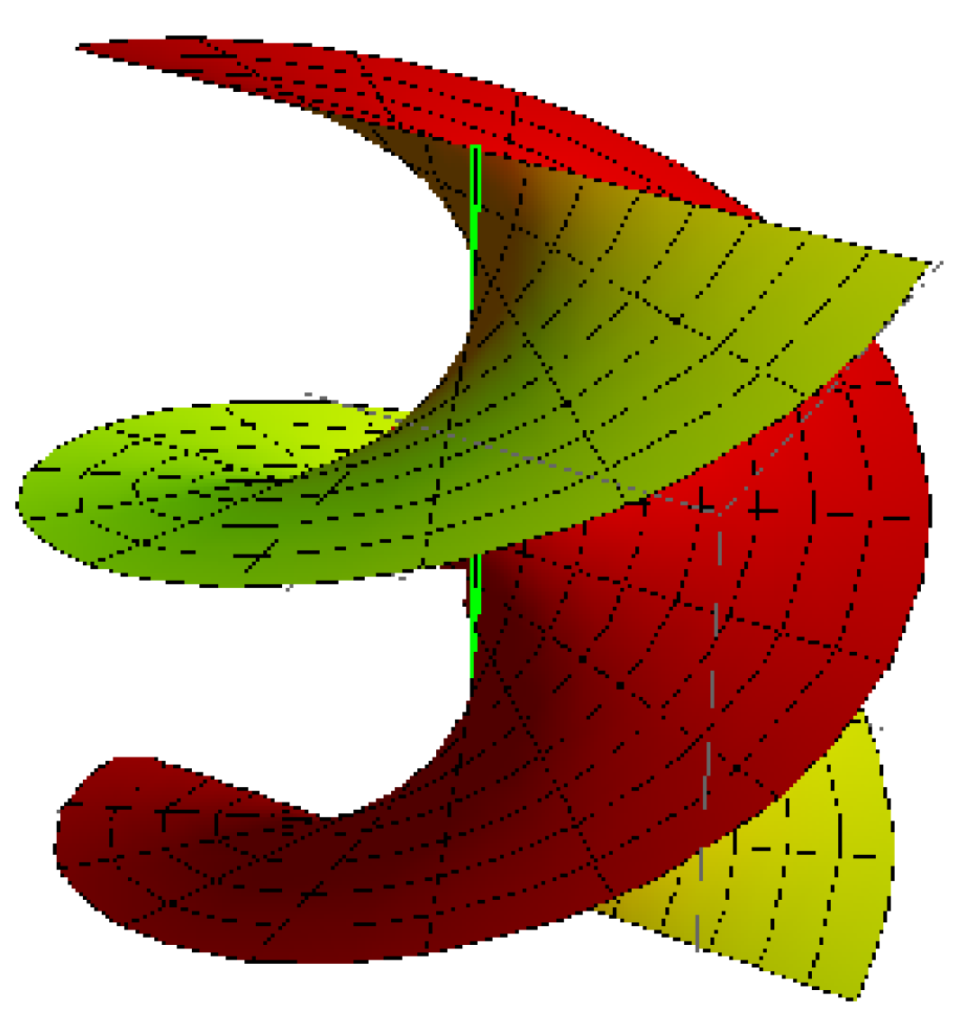
which is a one-parameter family of helicoidal surfaces. If we set $h=1$,$0\le u\le 2\pi$, and $-1\le t\le 1$, then an element of such a family can be attained (Figure 1).

Theorem 4. 

In the Euclidean 3-space ${\mathbb{E}}^3$, any right helicoidal surface belongs to inflection line congruence.

3.2. Procedure for Locating a Line Congruence

In this subsection, we offer a procedure for locating a line congruence from the coordinates of $\widehat{\mathbf{x}}$. Then, as a special case, we will induce the procedure for the inflection line congruence. From Equation (20), we have that ${\widehat{\mathbf{x}}}^{{}^{\prime }}$ is an orthogonal dual vector to both $\widehat{\mathbf{x}}$ and $\widehat{\omega }$; that is,

$$<\widehat{\mathbf{t}},{\widehat{\mathbf{r}}}_1>=<\widehat{\mathbf{t}},\widehat{\mathbf{x}}>=<\widehat{\mathbf{t}},\widehat{\mathbf{b}}>=0.$$

(38)

Then, the set {${\widehat{\mathbf{r}}}_1,\widehat{\mathbf{x}},\widehat{\mathbf{b}}$} constitutes a hyperbolic line congruence whose focus line is the line $\widehat{\mathbf{t}}$. We place $\widehat{\mathbf{t}}$ with respect to $\{{\widehat{\mathbf{r}}}_1,{\widehat{\mathbf{r}}}_2,{\widehat{\mathbf{r}}}_3\}$ by its restrict distance ${\phi }^{*}$, metrical through the $\mathbb{ISA}$ and the angle $\phi$ metrical with respect to ${\widehat{\mathbf{r}}}_2$. We insert the dual angles $\widehat{\vartheta }=\vartheta +\mathsf{\epsilon }{\vartheta }^{*}$ and $\widehat{\alpha }=\alpha +\mathsf{\epsilon }{\alpha }^{*}$, which display the locations of $\widehat{\mathbf{x}}$ and $\widehat{\mathbf{b}}$ along $\widehat{\mathbf{t}}$ (see Figure 2). Then,

$$\widehat{\mathbf{x}}=cos\widehat{\vartheta }{\widehat{\mathbf{r}}}_1+sin\widehat{\vartheta }\widehat{\mathbf{m}};\widehat{\mathbf{m}}=cos\widehat{\phi }{\widehat{\mathbf{r}}}_2+sin\widehat{\phi }{\widehat{\mathbf{r}}}_3.$$

(39)

From Equations (29) and (39), we attain

$$\left(\begin{array}{c}\widehat{\mathbf{x}}\hfill \\ \widehat{\mathbf{t}}\hfill \\ \widehat{\mathbf{g}}\hfill \end{array}\right)=\left(\begin{array}{ccc}cos\widehat{\vartheta }\hfill & sin\widehat{\vartheta }cos\widehat{\phi }\hfill & sin\widehat{\vartheta }sin\widehat{\phi }\hfill \\ 0\hfill & -sin\widehat{\phi }\hfill & cos\widehat{\phi }\hfill \\ sin\widehat{\vartheta }\hfill & -cos\widehat{\vartheta }cos\widehat{\phi }\hfill & -cos\widehat{\vartheta }sin\widehat{\phi }\hfill \end{array}\right)\left(\begin{array}{c}{\widehat{\mathbf{r}}}_1\hfill \\ {\widehat{\mathbf{r}}}_2\hfill \\ {\widehat{\mathbf{r}}}_3\hfill \end{array}\right).$$

(40)

Similarly, we have

$$\widehat{\mathbf{b}}=cos\widehat{\alpha }{\widehat{\mathbf{r}}}_1+sin\widehat{\alpha }\widehat{\mathbf{m}},$$

(41)

where $\widehat{\alpha }=\widehat{\vartheta }-\widehat{\psi }$. Notably, $\mathbf{s}$ is the origin of the relative Blaschke frame, that is, $\mathbf{s}=\mathbf{0}$, see Figure 2. This indicates that $\vartheta$ and ${\vartheta }^{*}$ are real constants. Via the real and the dual parts of $\widehat{\mathbf{x}}$ in Equation (39), we attain:

$$\left.\begin{array}{c}{x}_1=cos\vartheta ,x_1^{*}=-{\vartheta }^{*}sin\vartheta ,\hfill \\ x_2=sin\vartheta cos\phi ,x_2^{*}={\vartheta }^{*}cos\vartheta cos\phi -{\phi }^{*}sin\phi sin\vartheta ,\hfill \\ x_3=sin\vartheta sin\phi ,x_3^{*}={\phi }^{*}cos\vartheta sin\phi +{\phi }^{*}cos\phi sin\vartheta .\hfill \end{array}\right\}$$

(42)

Let a$(a_1,a_2,a_3)$ be a point on $\widehat{\mathbf{x}}$. Since ${\mathbf{x}}^{*}=$a$\times \mathbf{x}$, we have a system of linear equations in $a_i$ (i = 1, 2, 3, and $a_{is}$ are the coordinates of a):

$$\left.\begin{array}{c}\hfill a_{2}sin\vartheta sin\phi -a_{3}sin\vartheta cos\phi =x_1^{*},\hfill \\ \hfill -a_{1}sin\vartheta sin\phi +a_{3}cos\vartheta =x_2^{*},\hfill \\ \hfill a_{1}sin\vartheta cos\phi -a_{2}cos\vartheta =x_3^{*}.\hfill \end{array}\right\}$$

The matrix of coefficients of unknowns, $a_i$, is the skew symmetric matrix

$$\left(\begin{array}{ccc}0\hfill & sin\vartheta sin\phi \hfill & -sin\vartheta cos\phi \hfill \\ -sin\vartheta sin\phi \hfill & 0\hfill & cos\vartheta \hfill \\ sin\vartheta cos\phi \hfill & -cos\vartheta \hfill & 0\hfill \end{array}\right),$$

and thus its rank is 2 with $\vartheta \ne 2\pi k$ (k is an integer). The rank of the augmented matrix

$$\left(\begin{array}{cccc}0\hfill & sin\vartheta sin\phi \hfill & -sin\vartheta cos\phi \hfill & x_1^{*}\\ -sin\vartheta sin\phi \hfill & 0\hfill & cos\vartheta \hfill & x_2^{*}\\ sin\vartheta cos\phi \hfill & -cos\vartheta \hfill & 0\hfill & x_2^{*}\end{array}\right)$$

is also 2. Then, this system has infinite solutions specified by

$$\begin{array}{c}\hfill a_{2}sin\phi -a_{3}cos\phi =-{\vartheta }^{*}\hfill \\ \hfill a_2=(a_1-{\phi }^{*})tan\vartheta cos\phi -{\vartheta }^{*}sin\phi ,\hfill \\ \hfill a_3=(a_1-{\phi }^{*})tan\vartheta sin\phi +{\vartheta }^{*}cos\phi .\hfill \end{array}$$

Since $a_1$ can be arbitrary, then we may take $a_1={\phi }^{*}$. In this case, we have

$$\mathbf{a}(\phi ,{\phi }^{*})=({\phi }^{*},-{\vartheta }^{*}sin\phi ,{\vartheta }^{*}cos\phi ),$$

which is the base surface of the line congruence. Let $\mathbf{y}(y_1,y_2,y_3)$ be a point on the directed line $\widehat{\mathbf{x}}$, then

$$\left(\widehat{x}\right):\left.\begin{array}{c}{y}_1(\phi ,{\phi }^{*},v)={\phi }^{*}+vcos\vartheta ,\hfill \\ y_2(\phi ,{\phi }^{*},v)=-{\vartheta }^{*}sin\phi +vsin\vartheta cos\phi ,\hfill \\ y_3(\phi ,{\phi }^{*},v)={\vartheta }^{*}cos\phi +sin\vartheta sin\phi ,\hfill \end{array}\right\}$$

(43)

where $v\in \mathbb{R}$. Since $\phi$ and ${\phi }^{*}$ are two independent variables, we can say that ($\widehat{x}$), in general, is a line congruence in the ${\mathbb{L}}_f$ space. If we take ${\phi }^{*}=h\phi$ and $\phi$ as the movement parameter, then $\left(\widehat{x}\right)$ is ruled in the ${\mathbb{L}}_f$ space. As a result, the base surface reduces to the striction curve on ($\widehat{x}$), that is,

$$\mathbf{c}\left(\phi \right)=(h\phi ,-{\vartheta }^{*}sin\phi ,{\vartheta }^{*}cos\phi ).$$

The curvature ${\kappa }_c\left(\phi \right)$ and torsion ${\tau }_c\left(\phi \right)$ can be assigned by

$${\kappa }_c\left(\phi \right)=\frac{{\vartheta }^{*}}{{\vartheta }^{*2}+h^2},{\tau }_c\left(\phi \right)=\frac{h}{{\vartheta }^{*2}+h^2}.$$

Then, $\mathbf{c}\left(\phi \right)$ is a cylindrical helix along the $\mathbb{ISA}$, and the ruled surface is

$$\left(\widehat{x}\right):\left.\begin{array}{c}{y}_1(\phi ,v)=h\phi +vcos\vartheta ,\hfill \\ y_2(\phi ,v)=-{\vartheta }^{*}sin\phi +vsin\vartheta cos\phi ,\hfill \\ y_3(\phi ,v)={\vartheta }^{*}cos\phi +sin\vartheta sin\phi .\hfill \end{array}\right\}$$

(44)

The constants h, $\vartheta$, and ${\vartheta }^{*}$ can control the situation of the surface $\left(\widehat{x}\right)$. In the case where $0\le \phi \le 2\pi$ and ${\vartheta }^{*}\ne 0$, we attain:

$$\left(\widehat{x}\right):-\frac{Y_1^2}{{\varrho }^2}+\frac{y_2^2}{{\vartheta }^{*2}}+\frac{y_3^2}{{\vartheta }^{*2}}=1,$$

(45)

where $\varrho ={\vartheta }^{*}cot\vartheta$ and $Y_1=y_1-h\phi$. Thus, $\left(\widehat{x}\right)$ is a two-parameter hyperboloid of one sheet. The intersection of each hyperboloid and the plane $y_1=h\phi$ is a one-parameter family of cylinders $\left(c\right)$: $y_2^2+y_3^2={\vartheta }^{*2}$, which is the envelope of $\left(\widehat{x}\right)$. Furthermore, the ruled surface $\left(\widehat{x}\right)$ can be separated as follows:

(1)

An Archimedes helicoid, where its striction curve is a cylindrical helix, for $h={\vartheta }^{*}=0.5$, $\vartheta =\frac{\pi }{4}$, $-3\le v\le 3$, and $0\le \phi \le 2\pi$ (Figure 3).

(2)

A hyperboloid of one sheet, where its striction curve is a circle, for $h=0,$${\vartheta }^{*}=0.5$, $\vartheta =\frac{\pi }{4}$, $-3\le v\le 3$, and $0\le \phi \le 2\pi$ (Figure 4).

(3)

A right helicoid, where its striction curve is a line, for $h=1$, ${\vartheta }^{*}=0$, $\vartheta =\frac{\pi }{2}$, $-3\le v\le 3$, and $0\le \phi \le 2\pi$ (Figure 5).

(4)

A cone, where its striction curve is a stationary point, for $h={\vartheta }^{*}=0$, $\vartheta =\frac{\pi }{4}$, $-2\le v\le 2$, and $0\le \phi \le 2\pi$ (Figure 6).

Figure 3. Archimedes helicoid.

Figure 3. Archimedes helicoid.

Figure 4. A hyperboloid of one sheet.

Figure 4. A hyperboloid of one sheet.

Figure 5. A right helicoid.

Figure 5. A right helicoid.

Figure 6. A cone.

Figure 6. A cone.

Explanations of the Inflection Line Congruence

For the kinematic differential geometry of the inflection line congruence, from Equation (31), we have

$$\widehat{c}:{\widehat{x}}_1\widehat{\omega }(1-{\widehat{x}}_1^2)+{\widehat{x}}_3=0.$$

(46)

Equation (46) is the dual inflection point trajectory in spherical kinematics (compared with [1,2,3]). This spherical recognition is a dual spherical curve of the third degree. The real part of Equation (46) displays the inflection cone as

$$c:x_1\omega (1-x_1^2)+x_3=0.$$

(47)

The meeting of the inflection cone with a real unit sphere fixed at the peak of the cone demonstrates a spherical curve. The dual part of Equation (42) demonstrates the linked plane of lines:

$$\pi :(1-x_1^2)\left(x_1{\omega }^{*}+\omega x_1^{*}\right)-2x_1\omega x_2{x}_2^{*}+x_3^{*}=0.$$

(48)

Furthermore, if we substitute Equation (46) into Equations (47) and (48), respectively, we attain

$$c:\omega sin2\vartheta +2sin\phi =0$$

(49)

and

$$\pi :{\omega }^{*}sin2\vartheta +2\omega {\vartheta }^{*}cos2\vartheta +2{\phi }^{*}cos\phi =0.$$

(50)

If Equation (49) is solved with respect to $\phi$, we gain

$$sin\phi =-\frac{\omega sin2\vartheta }{2},\mathrm{and}cos\phi =\pm \frac{1}{2}\sqrt{4-{\left(\omega sin2\vartheta \right)}^2}.$$

(51)

From Equations (51) and (50), we find

$$\pi :{\omega }^{*}sin2\vartheta +2\omega {\vartheta }^{*}cos2\vartheta \pm {\phi }^{*}\sqrt{4-{\left(\omega sin2\vartheta \right)}^2}=0.$$

(52)

Equation (52) is linear in the coordinates ${\phi }^{*}$ and ${\vartheta }^{*}$ of $\widehat{\mathbf{x}}$. Thus, for a one-parameter spatial movement ${\mathbb{L}}_m/{\mathbb{L}}_f$, the lines in a given stationary direction in the ${\mathbb{L}}_m$ space lie on a plane. As shown in Figure 7, the angle $\phi$ identifies the central normal $\widehat{\mathbf{t}}$; thus, Equation (52) defines two lines $L^{+}$ and $L^{-}$ in the plane spanned by $\widehat{\mathbf{t}}$ and the $\mathbb{ISA}$ ($L^{+}$ and $L^{-}$ are conformable to the inflection circle in planar kinematics). If the distance ${\phi }^{*}$ over the $\mathbb{ISA}$ is taken as the independent parameter, then Equation (52) becomes

$$\pi :{\vartheta }^{*}=\mp \frac{\sqrt{4-{\left(\omega sin2\vartheta \right)}^2}}{2\omega cos2\vartheta }{\phi }^{*}-htan2\vartheta ,$$

(53)

where $4-{\left(\omega sin2\vartheta \right)}^2\ge 0$. Equation (53) displays that the two lines $L^{+}$ and $L^{-}$ intersect the $\mathbb{ISA}$ at a distance of $-htan2\vartheta$. for $\vartheta =0$ these lines are through $\mathbf{s}$, and their achieve their minimum slope $m=\mp \omega$. Furthermore, $L^{+}$ (or $L^{-})$ will change its place if $\vartheta$ is realized as a varying value and $\phi$ is a constant. Furthermore, the place of the plane $\pi$ changes if the variable $\phi$ of $L^{+}$ (or $L^{-})$ has several values and $\vartheta$ is a constant. Therefore, the set of all lines $L^{+}$ and $L^{-}$ realized by Equation (53) is an inflection line congruence for all values of $({\phi }^{*},{\vartheta }^{*})$ (Figure 7).

Now, it is simple to explain a parametric equation of the ruled surface in the inflection line congruence. For this objective, from the real part of Equation (39) and from Equation (51), we obtain

$$\mathbf{x}\left(\vartheta \right)=\left(cos\vartheta ,\frac{1}{2}\sqrt{4-{\left(\omega sin2\vartheta \right)}^2}sin\vartheta ,-\frac{\omega sin2\vartheta }{2}\vartheta sin\vartheta \right),$$

(54)

which is the inflection curve of the spherical part of the movement ${\mathbb{L}}_m/{\mathbb{L}}_f$. From Equations (44) and (51), we attain

$$\mathbf{y}(\vartheta ,v)=\left(\begin{array}{c}h{sin}^{-1}\left(-\frac{\omega sin2\vartheta }{2}\right)+vcos\vartheta \\ {\vartheta }^{*}\left(\frac{\omega sin2\vartheta }{2}\right)+v\frac{1}{2}\sqrt{4-{\left(\omega sin2\vartheta \right)}^2}sin\vartheta \\ {\vartheta }^{*}\frac{1}{2}\sqrt{4-{\left(\omega sin2\vartheta \right)}^2}-\frac{v}{2}\omega sin2\vartheta sin\vartheta \end{array}\right),v\in \mathbb{R},$$

(55)

where h, $\omega$, and ${\vartheta }^{*}$ can control the shape of the surface $\left(\widehat{x}\right)$. Furthermore, for example, from Equations (54) and (55), we have:

(1)

An inflection curve and a ruled surface with a striction curve for $h={\vartheta }^{*}=1$, $\omega =1$, $-2\le v\le 0$, and $0\le \vartheta \le 2\pi$ (Figure 8 and Figure 9).

(2)

An inflection curve and a ruled surface with a striction curve for $h={\vartheta }^{*}=1$, $\omega =1.5$, $-2\le v\le 0$, and $0\le \phi \le 2\pi$ (Figure 10 and Figure 11).

Figure 8. Inflection curve.

Figure 8. Inflection curve.

Figure 9. Ruled surface.

Figure 9. Ruled surface.

Figure 10. Inflection curve.

Figure 10. Inflection curve.

Figure 11. Ruled surface.

Figure 11. Ruled surface.

3.3. Euler–Savary Equation and Disteli Formulae

In 1914, Disteli [9] succeeded in locating a curvature axis for the generating line of a ruled surface and established the Euler–Savary equation in spatial kinematics. The Disteli formulae may be gained directly by calculating the dual spherical curvature of $\widehat{\mathbf{x}}\left(\widehat{u}\right)$ as follows. The dual spherical radius of curvature $\widehat{\psi }$ can be written as (see Figure 2):

$$\widehat{\psi }=\widehat{\vartheta }-\widehat{\alpha }\iff \varphi =\vartheta -\alpha ,{\varphi }^{*}={\vartheta }^{*}-{\alpha }^{*}.$$

(56)

Then, we have the identity

$$\widehat{\chi }(\widehat{u}):=cot\widehat{\psi }=cot(\widehat{\vartheta }-\widehat{\alpha }).$$

(57)

From substituting Equations (34) and (39) into Equation (57), we acquire

$$cot(\widehat{\vartheta }-\widehat{\alpha })=cot\widehat{\vartheta }+\frac{sin\widehat{\phi }}{\widehat{\omega }{sin}^2\widehat{\vartheta }}.$$

After some algebraic manipulations, this becomes

$$cot\widehat{\alpha }-cot\widehat{\vartheta }=\frac{\widehat{\omega }}{sin\widehat{\phi }}.$$

(58)

Equation (58) is a dual spherical Euler–Savary equation (compared with [1,2,3]). Via the real and the dual parts, respectively, we get

$$cot\alpha -cot\vartheta =\frac{\omega }{sin\phi }$$

(59)

and

$${\phi }^{*}=[h-(\frac{{\vartheta }^{*}}{{sin}^2\vartheta }-\frac{{\alpha }^{*}}{{sin}^2\alpha })\frac{sin\phi }{\omega }]tan\phi .$$

Equations (59) and (60) are new Disteli formulae in a one-parameter spatial movement; the first one reveals the relationship between the places of the stationary line $\widehat{\mathbf{x}}$ in the movable space ${\mathbb{L}}_m$ and the Disteli axis $\widehat{\mathbf{b}}$. The second one identifies the distance from the line $\widehat{\mathbf{x}}$ to the Disteli axis $\widehat{\mathbf{b}}$.

At the end of this section, we derive a dual Euler–Savary formula for the axodes as follows. Substituting $\widehat{\vartheta }={\widehat{\phi }}_m$, $\widehat{\alpha }={\widehat{\phi }}_f$, $\phi =\frac{\pi }{2}$, and ${\phi }^{*}=0$ into Equation (58), we find, after simple simplifications, that

$$cot{\widehat{\phi }}_f-cot{\widehat{\phi }}_m=\widehat{\omega }.$$

(60)

This is a dual form of a well-known Euler–Savary formula from ordinary spherical kinematics [1,2,3]. This dual version identifies an association between the two axodes in immediate contact and the kinematic geometry corresponding to the instantaneous invariants of the movement ${\mathbb{L}}_m/{\mathbb{L}}_f$. From separating the real and the dual parts, respectively, we find

$$cot{\phi }_f-cot{\phi }_m=\omega$$

(61)

and

$$\frac{{\phi }_m^{*}}{{sin}^2{\phi }_m}-\frac{{\phi }_f^{*}}{{sin}^2{\phi }_f}={\omega }^{*}.$$

(62)

Equation (61) together with Equation (62) are novel Disteli formulae for the axodes of the movement ${\mathbb{L}}_m/{\mathbb{L}}_f$.

4. Conclusions

This paper studies the kinematic differential geometry of a line trajectory in spatial movement at any instant via the relative movements of two dual unit spheres. A line trajectory is represented by the invariants of axodes of a rigid body in spatial movement. The Disteli formulae of a line trajectory in spatial movement are described and concise expressions of the inflection line congruence are acquired. Hopefully, these results will lead to a wider usage of the geometric properties of ruled surfaces traced by lines embedded in spatial mechanisms. In future work, we plan to research some applications of kinematic geometry of one-parameter spatial movements combined with singularity theory, submanifold theory, etc., in [19,20] to find more new results and properties.

References

1. Bottema, O.; Roth, B. Theoretical Kinematics; North-Holland Press: New York, NY, USA, 1979. [Google Scholar]
2. Karger, A.; Novak, J. Space Kinematics and Lie Groups; Gordon and Breach Science Publishers: New York, NY, USA, 1985. [Google Scholar]
3. Schaaf, J.A. Curvature Theory of line Trajectories in Spatial Kinematics. Ph.D. Thesis, University of California, Davis, CA, USA, 1988. [Google Scholar]
4. Stachel, H. Instantaneous Spatial Kinematics and the Invariants of the Axodes; Technical Report 34; Institute fur Geometrie: TU Wien, Austria, 1996. [Google Scholar]
5. Pottman, H.; Wallner, J. Computational Line Geometry; Springer: Berlin/Heidelberg, Germany, 2001. [Google Scholar]
6. Garnier, R. Cours de Cinématique, Tome II: Roulement et Vibration-La Formule de Savary et Son Extension a l’Espace; Gauthier-Villars: Paris, France, 1956. [Google Scholar]
7. Phillips, J.; Hunt, K. On the theorem of three axes in the spatial motion of three bodies. J. Appl. Sci. 1964, 15, 267–287. [Google Scholar]
8. Skreiner, M. A study of the geometry and the kinematics of Instantaneous spatial motion. J. Mech. 1966, 1, 115–143. [Google Scholar] [CrossRef]
9. Dizioglu, B. Einfacbe Herleitung der Euler–Savaryschen Konstruktion der riiumlichen Bewegung. Mech. Mach. Theory 1974, 9, 247–254. [Google Scholar] [CrossRef]
10. Köse, Ö.; Sarıoglu, C.C.; Karabey, B.; Karakılıç, I. Kinematic differential geometry of a rigid body in spatial motion using dual vector calculus: Part-II. Appl. Math. 2006, 182, 333–358. [Google Scholar] [CrossRef]
11. Abdel-Baky, R.A.; Al-Ghefari, R.A. On the one-parameter dual spherical motions. Comput. Aided Geom. Des. 2011, 28, 23–37. [Google Scholar] [CrossRef]
12. Turhan, T.; Ayyıldız, N. A study on geometry of spatial kinematics in Lorentzian space. Süleyman Demirel Üniv. Fen Bilim. Enstitüsü Derg. 2017, 21, 808–811. [Google Scholar] [CrossRef]
13. Aslan, S.; Bekar, M.; Yaylı, Y. Ruled surfaces corresponding to hyper-dual curves. Hacet. J. Math. Stat. 2022, 51, 187–198. [Google Scholar] [CrossRef]
14. Aslan, M.C.; Sekerci, G.A. Dual curves associated with the Bonnet ruled surfaces. Int. J. Geom. Methods Mod. Phys. 2020, 17, 050204. [Google Scholar]
15. Alluhaibi, N. Ruled surfaces with constant Disteli-axis. AIMS Math. 2020, 5, 7678–7694. [Google Scholar] [CrossRef]
16. Abdel-Baky, R.A.; Tas, F. W-Line congruences. Commun. Fac. Sci. Univ. Ank. Ser. A1 Math. Stat. 2020, 69, 450–460. [Google Scholar] [CrossRef]
17. Hussein, R.A.; Ali, A.A. Geometry of the line space associated with a given dual ruled surface. AIMS Math. 2022, 7, 8542–8557. [Google Scholar] [CrossRef]
18. Aydinalp, M. The forward kinematics of dual rulling contact of one dual unit sphere on another with dual Darboux frame based equation. Hacet. J. Math. Stat. 2021, 50, 1583–1594. [Google Scholar] [CrossRef]
19. Li, Y.; Aldossary, M.T.; Abdel-Baky, R.A. Spacelike circular surfaces in Minkowski 3-space. Symmetry 2023, 15, 173. [Google Scholar] [CrossRef]
20. Li, Y.; Chen, Z.; Nazra, S.H.; Abdel-Baky, R.A. Singularities for timelike developable surfaces in Minkowski 3-Space. Symmetry 2023, 15, 277. [Google Scholar] [CrossRef]
Figure 1. Helicoidial surface.
Axioms 12 00472 g001
Figure 2. Relative positions of x ^ and b ^ .
Axioms 12 00472 g002
Figure 7. Inflection line congruence.
Axioms 12 00472 g007
Disclaimer/Publisher’s Note: The statements, opinions and data contained in all publications are solely those of the individual author(s) and contributor(s) and not of MDPI and/or the editor(s). MDPI and/or the editor(s) disclaim responsibility for any injury to people or property resulting from any ideas, methods, instructions or products referred to in the content.