Abstract
A linear transformation from vector space to another vector space can be represented as a matrix. This close relationship between the matrix and the linear transformation is helpful for the study of matrices. In this paper, the tensor is regarded as a generalization of the matrix from the viewpoint of the linear transformation instead of the quadratic form in matrix theory; we discuss some operations and present some definitions and theorems related to tensors. For example, we provide the definitions of the triangular form and the eigenvalue of a tensor, and the theorems of the tensor QR decomposition and the tensor singular value decomposition. Furthermore, we explain the significance of our definitions and their differences from existing definitions.
MSC:
15A69; 53A45; 15A18
1. Introduction
Unfolding is an important approach in tensor research, and one of the common methods of unfolding is mode-n matricization. Based on this, the mode-n product and n-rank are defined. This helps to extend the concepts of the eigenvalue and the singular value decomposition of matrices to tensors. For example, the eigenvalues of a real supersymmetric tensor are presented in [1], a multilinear singular value decomposition (HOSVD) is presented in [2], and the restricted singular value decomposition (RSVD) for three quaternion tensors is presented in [3]. The singular values of the general tensor are introduced in [4]. In [5,6], the singular values of a tensor are connected with its symmetric embedding. In [7], the authors presented the definition of the singular value of a real rectangular tensor and discussed its properties. For a tensor , exploiting the matricization of the tensor, a singular value decomposition is presented in [8]. On the other hand, in matrix theory, many studies of matrices are inseparable from linear transformations. Due to the one-to-one correspondence between matrices and linear transformations, we always believe that it is more natural to provide definitions and theorems related to tensors from the viewpoint of linear transformation. This fact also proves that when we think from this perspective, some unresolved tensor problems have already been solved. Similar studies have been considered in [9]. We provide some supplements to the article presented in [9]; for example, we give a more general definition of the multiplication between tensor and tensor and present the form of a triangular tensor by proposing tensor QR decomposition. In addition, in matrix theory, the one-dimensional linear subspace made up of the eigenvectors of one eigenvalue of a linear transformation is stable under the action of this linear transformation. However, this property cannot be generalized for the existing tensor eigenvalue and the corresponding eigenvector. From this point of view, we present a new concept of the eigenvalue and the corresponding eigenvector of an even-order tensor. Then, the concepts of the eigenvalue decomposition, singular value, and singular value decomposition are naturally obtained.
This paper is organized as follows. In Section 2, regarding the tensor as a linear transformation, we present some definitions. For example, we present the identity tensor and a new multiplication for two tensors, and further explain the partitioning of the indices of a tensor. In Section 3, starting from the orthogonalization process of a set of tensors, we present the QR decomposition of a tensor and the form of a triangular tensor. In Section 4, motivated by the invariant eigenspace, we derive the definitions of the tensor eigenvalue and the corresponding tensor eigenvector, and the spectral decomposition theorem of a Hermitian tensor. The singular value decomposition of a tensor is defined in Section 5, and numerical examples are used to illustrate the advantages of our singular value decomposition in tensor compression. The application of the tensor singular value decomposition is described in Section 6.
2. Basic Definitions
For the convenience of writing, we illustrate the symbols to be used, which are similar to those in [9]. The set of integers will be abbreviated to the symbol henceforth. Let denote a partitioning of the set , where and are two disjointed nonempty subsets that satisfy . Additionally, let denote the number of elements in the set . Under a given partitioning , an element in the tensor T will be marked as , where , and , for all and .
Given a partitioning , an order-p tensor can be regarded as a linear map
In particular, an identity map is a linear transformation
that can map each tensor to itself, in other words, for arbitrary , . Because the relationship between a tensor and the corresponding linear transformation depends on the partitioning , in order to avoid confusion, we note the tensor discussed under the partitioning as . When T and are known, we can use a command in MATLAB to determine directly [10],
T_alpha_beta = permute(T,[alpha,beta]),
where [alpha,beta] indicates the order of the subscripts to be accessed when performing identification. In fact, for a fixed partitioning , the tensor can be restored as a matrix. Precisely speaking, the element of an order-p tensor is saved at location of a matrix, where
This storage method can also be regarded as a special case of blocking in [11].
Definition 1
([11]). The set is a blocking for if is a vector of positive integers that sums to for .
When is a vector with ones in all elements and of length for all , and for all , the blocking M is the row blocking of under the partitioning . Similarly, we can obtain the column blockings. Specifically, the entry of an order-p tensor can also be saved at the location
of the linear array. In the subsequent discussion, we shall comply with the rules in (1) or (2) whenever we want to unfold a tensor to a matrix or a vector.
There are many ways to define multiplication between tensors [12]. Based on the relationship between a tensor T and the corresponding map , in [9], the authors defined the tensor multiplication between the tensor T and any lower-order tensor as follows
The adjoint of , denoted by , is a linear transformation
such that the Lagrange identity [13]
is satisfied for all and . The tensor representation of the linear transformation is , which is the conjugate transposition of . See [9] for more details.
Similar to the derivation of the multiplication in (3), by means of linear transformation, we define another multiplication between two tensors G and T when there exists and satisfying and . This definition is a generalization of the existing tensor contraction definition.
Definition 2.
Suppose the linear transformations corresponding to G and T are
then, the composition of and is a linear transformation
The rule of action is
where , . The corresponding tensor form is , where , and
From this, we can present the following theorem:
Theorem 1.
Let and be the linear transformations defined in (4) and let and be their tensor representations. Denote the adjoints of and by and and the conjugate transposes of and by and , respectively. Then,
Proof.
For any , , we have
From the arbitrariness of A and B, we can obtain . Because the tensors and are the tensor representations of the linear transformations and , respectively, the equation can be established immediately. □
3. QR Decomposition of the Tensor
QR decomposition is a fundamental tool in matrix theory and plays an important role in the design of algorithms. In this section, we aim to present the tensor QR decomposition of a given tensor from the perspective of linear transformation and describe the form of the triangular tensor based on it.
For the given tensor T, the partitioning and the multi-index , the process of orthogonalizing the tensors is similar to the Gram–Schmidt orthogonalization process of the column vectors of a matrix. In this orthogonalization process, the tensor T and the tensors play the roles of the matrix and column vectors, respectively. Suppose the only way to obtain is for all the scalars to be zero. The orthogonalization process of the tensors then works as follows:
where . In general, we have
where . Equation (6) can be rewritten as
where . This expression leads us to obtain a tensor decomposition
where satisfies
satisfies
and means
Example 1.
Consider the order-4 tensor with the partitioning . Applying the orthogonalization process, we can obtain the QR decomposition of T. The tensors can be laid out, respectively, as the "matrix" of blocks of matrices
and
When the tensor is an order-2 tensor, the QR decomposition of the tensor degenerates into the QR decomposition of the matrix. This is also in line with the fact that tensors are higher-order generalizations of matrices.
Based on the above QR decomposition, we can obtain the following definitions of triangular tensors, which are generalizations of those in matrix theory and different from those in [14].
Definition 3.
For a given tensor and a partitioning , we call T upper triangular (or, lower triangular, diagonal) under the partitioning if whenever
The elements satisfying
are the diagonal elements, where means the index satisfies
Example 2.
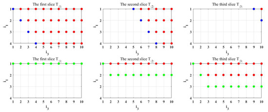
For a tensor with the partitioning , we mark its diagonal elements and upper triangular elements at the first row of Figure 1 for observation convenience, where the blue dots represent diagonal elements, and the red dots represent the strictly upper triangular elements. Additionally, we mark the upper triangular elements and the strictly upper triangular elements defined by [14] at the second row of Figure 1, where the red dots represent the strictly upper triangular elements, and the green and red dots together form the upper triangle elements. The slices in the figure are lateral slices [12], and the indices of the elements of T are denoted as .
Figure 1.
Upper triangular elements under different definitions.
4. Eigenvalue of the Tensor
The eigeninformation of a matrix is a fundamental concept in the field of matrix analysis and plays an important role in many practical applications. Therefore, it is necessary to consider the definition and existence of the eigeninformation of a tensor.
In linear algebra, if there exists a constant and a nonzero vector such that , we call the eigenvalue of A, and call the eigenvector associated with . The equation is bilinear and implies that the one-dimensional linear subspace expanded by eigenvectors associated with the same eigenvalue remains stable under the corresponding linear transformation. However, H-eigenvalues and Z-eigenvalues do not keep this property. With the benefit of the linear transformation, we present a new definition of the eigeninformation of an even-order tensor.
Firstly, we propose a new concept of square tensors from the viewpoint of an identity map, which is different from the definitions in [9,12].
Definition 4.
For the tensor , if there exists a partitioning satisfying and , then we call the tensor T a square tensor under the partitioning .
Definition 5.
Suppose is a square tensor under the partitioning , then we have a transformation . We call an -eigenvalue of T, or an -eigenvalue of , if when partnered with a nonzero tensor it satisfies
and the tensor X is called an -eigentensor of T associated with the eigenvalue λ.
This definition is similar to that in [15], which conforms to our original intention of proposing the new definition of the tensor eigenvalue. The linear invariance of matrix eigensubspace is generalized.
Theorem 2.
Suppose are all eigentensors associated with the eigenvalue λ of the tensor T and are complex numbers. Then, is also the eigentensor associated with the eigenvalue λ of the tensor T.
Proof.
Because are all eigentensors associated with the eigenvalue , . Then,
Thus, the theorem has been proven. □
It is worth noting that for an order-4 tensor, if the elements of T satisfy , the eigenvalues of T under the partitioning and the partitioning are the same. Extending the conclusion to the general situation, we obtain that if is square under the partitioning and and satisfies , then the eigenvalues of T under the partitioning and the partitioning are the same. Importantly, if T is a supersymmetric tensor, the eigenvalues under arbitrary partitioning that satisfy are the same.
For a square tensor under the partitioning , if its corresponding transformation satisfies , we call the transformation a self-adjoint operator and call the tensor a Hermitian tensor under the partitioning [9]. Based on this concept, and similar to the spectral theorem of a symmetric matrix, we present and prove the following lemma and theorem.
Lemma 1.
Suppose the tensor is Hermitian under the partitioning , then the -eigentensors corresponding to different -eigenvalues of T are orthogonal.
Proof.
Let and be two different -eigenvalues of T, where and are -eigentensors corresponding to and , respectively. Then, , . Therefore,
Because , . □
Theorem 3.
Suppose the tensor is Hermitian under the partitioning . Then, it has the decomposition
where is a unitary tensor [9], and is a diagonal tensor whose diagonal elements are the eigenvalues under the partitioning of T.
Proof.
Let be the -eigenvalues of T, and let be the corresponding -eigentensors, where . Then,
Therefore,
The results from Lemma 1 demonstrate that, when , the above equation is equal to ; otherwise, it is equal to 0. Furthermore, it can be concluded that ; thus, the theorem has been proven. □
5. Singular Value Decomposition of the Tensor
Based on the eigenvalue of a tensor in Section 4, we want to offer a new definition of tensor singular value decomposition, which is a generalization of the decomposition in [8]. To sufficiently demonstrate the feasibility of this decomposition, we first propose the following theorem and definition.
Theorem 4.
All the eigenvalues of or are non-negative.
Proof.
Suppose that is an arbitrary eigenpair of , so it is also an eigenpair of . Then, we can obtain
Because and , we have . From the arbitrariness of the eigenpair, we can see that all the eigenvalues of are non-negative. □
Definition 6.
For a tensor with the partitioning , we call the non-negative square root of an eigenvalue of a singular value under the partitioning of the tensor T.
Theorem 5.
Each tensor with the partitioning has a singular value decomposition under the partitioning (SVDUP)
in which and are the unitary tensors, and is a diagonal tensor whose diagonal elements are the singular values under the partitioning of T.
Proof.
Without loss of generality, we only prove the case when . is a Hermitian tensor. From Theorem 3, it can be seen that there is a unitary tensor and diagonal tensor satisfying
Let be a diagonal tensor whose diagonal elements are the square roots of the diagonal elements of . Let be the tensor by adding or deleting zeros in the tensor . is a tensor satisfying the linear equation , that is, . Finally, we use the appropriate tensors that constitute the unitary tensor together with . □
When , T is a second-order tensor, in decomposition (9), U and V are matrices. It is clear that SVDUP is a generalization of matrix singular value decomposition in order. Therefore, we unify the concepts of a tensor singular value and unique left and right singular tensors. For the singular value decomposition of a matrix, the core matrix is a diagonal matrix, but the core tensor of HOSVD [2] is not. Additionally, it is impossible to transform higher-order tensors into a pseudodiagonal tensor by performing orthogonal transformations [2]. From this perspective, our definition would be a better way to generalize the singular value decomposition of matrices. In addition, to demonstrate the advantages of our SVDUP method in data compression, we also provide the following example.
Example 3.

We randomly generate tensors using the command “create_problem” in the Tensor Toolbox, and compress them using truncated SVDUP and truncated HOSVD, respectively. Then, we compare the accuracy while ensuring that the compression ratio is almost the same in advance. In order to guarantee the generality of the experiment, we test 1000 data points of each size. The metric [16]
where and are the approximations of T computed by truncated SVDUP and truncated HOSVD, respectively, is introduced to describe the accuracy of the approximations. means can provide a more accurate approximation. The compression ratio is equal to the number of elements contained in the approximate tensor divided by the number of elements in the original tensor. p represents order, and I represents dimension of each order.
Table 1 and Table 2 illustrate that as the tensor scale increases, our T-SVDUP can obtain higher accuracy approximations than T-HOSVD under a similar compression ratio.
Table 1.
Comparison between T-SVDUP and T-HOSVD with .
Table 2.
Comparison between T-SVDUP and T-HOSVD with .
6. Application
In both academic research and practical applications, there are many examples of mapping elements in one high-dimensional space to another. For example, a color image is mapped to a blurred image in 3D space during image processing, one discrete matrix is mapped to another in the process of the discretization of Poisson’s equation, and so on. The existing processing method is to stretch data into vectors, but the structure of the data is destroyed this way. In this section, we take two-dimensional image deblurring as an example to describe the application of SVDUP without the destruction of data structure.
In order to calculate the pixels of the blurred pixel matrix Y, we should rotate the PSF (point spread function) array 180 degrees and match it with the pixels in the source pixel matrix X by placing the center of the rotated PSF array on the pixels of X [17]. Then, the products of the corresponding components are summed to be . For example, let , and be the PSF array, the source pixel matrix and the blurred pixel matrix, respectively. Then,
Particularly, if we assume zero boundary conditions, the elements at the border of Y are given by
We assume to be the map from the source pixel matrix to the blurred pixel matrix. Then, the element of its tensor representation T is
Then, the transformation can be summarized as . The image deblurring problem is recovering the source pixel matrix X from the blurred pixel matrix , where is a kind of noise.
We use the SVDUP to analyze this problem. The solution can be written as
where , , , satisfying , and is the singular value satisfying . In general, for the blurring tensor, , and the number is large. The approach that is frequently used to dampen the effects of small singular values is to discard all SVDUP components with small singular values, that is, constructing the approximation
where is smaller than the given tolerance. This method is called the truncated SVDUP, which is a particular case of the spectral filtering methods
where the filter factors are chosen such that for large singular values, and for small singular values [17]. To some extent, this method can compensate for the errors caused by the truncation of singular values.
Suppose the original image is blurred with a circular averaging blur kernel, and perturbed by Gaussian white noise. Figure 2 shows the image recovered using truncated SVDUP with different truncations. All of our computations were performed in MATLAB 2016a running on a PC Intel(R) Core(TM) i7-7500 of 2.7 GHZ CPU and 8 GB of RAM.
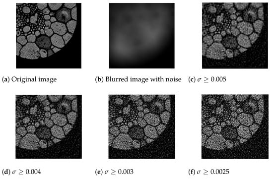
Figure 2.
Deblurring with different truncations.
7. Conclusions
In this paper, from the perspective of linear transformation, we present some basic concepts and provide three tensor decompositions: QR decomposition, spectral decomposition and singular value decomposition. These concepts and decompositions are different from the existing results and are more natural generalizations of the corresponding matrix theory. The numerical results also show the effectiveness of our new decomposition method.
Author Contributions
Conceptualization, B.Y. and B.D.; methodology, X.Z. and B.D.; software, X.Z.; writing—original draft preparation, X.Z and B.D.; writing—review and editing, X.Z. and Y.Y.; funding acquisition, Y.Y., B.Y., B.D. and X.Z. All authors have read and agreed to the published version of the manuscript.
Funding
This work was supported in part by the National Natural Science Foundation of China (Grant Nos. 11871136, 11971092 and 11801382), Natural Science Foundation of Liaoning Province, China (Grant Nos. 2020-MS-278 and 2023-MS-142), Scientific Research Foundation of Education Department of Liaoning Province, China (Grant Nos. 2020JYT04, LJKZ0096 and LJKMZ20220452).
Data Availability Statement
Data sharing not applicable to this paper, as no data sets were generated or analyzed during the current study.
Conflicts of Interest
The authors declare no conflict of interest.
References
- Qi, L. Eigenvalues of a real supersymmetric tensor. J. Symbolic Comput. 2005, 40, 1302–1324. [Google Scholar] [CrossRef]
- De Lathauwer, L.; De Moor, B.; Vandewalle, J. A multilinear singular value decomposition. SIAM J. Matrix Anal. Appl. 2000, 21, 1253–1278. [Google Scholar] [CrossRef]
- Chen, W.J.; Yu, S.W. RSVD for Three Quaternion Tensors with Applications in Color Video Watermark Processing. Axioms 2023, 12, 232. [Google Scholar] [CrossRef]
- Lim, L.H. Singular values and eigenvalues of tensors: A variational approach. In Proceedings of the IEEE International Workshop on Computational Advances in Multi-Sensor Adaptive Processing, Puerto Vallarta, Mexico, 13–15 December 2005; pp. 129–132. [Google Scholar]
- Chen, Z.; Lu, L. A tensor singular values and its symmetric embedding eigenvalues. J. Comput. Appl. Math. 2013, 250, 217–228. [Google Scholar] [CrossRef]
- Ragnarsson, S.; Van Loan, C.F. Block tensors and symmetric embeddings. Linear Algebra Appl. 2013, 438, 853–874. [Google Scholar] [CrossRef]
- Chang, K.; Qi, L.; Zhou, G. Singular values of a real rectangular tensor. J. Math. Anal. Appl. 2010, 370, 284–294. [Google Scholar] [CrossRef]
- Brazell, M.; Li, N.; Navasca, C.; Tamon, C. Solving multilinear systems via tensor inversion. SIAM J. Matrix Anal. Appl. 2013, 34, 542–570. [Google Scholar] [CrossRef]
- Guan, Y.; Chu, M.T.; Chu, D. SVD-based algorithms for the best rank-1 approximation of a symmetric tensor. SIAM J. Matrix Anal. Appl. 2018, 39, 1095–1115. [Google Scholar] [CrossRef]
- Li, L.; Victoria, B. MATLAB User Manual; MathWorks: Natick, MA, USA, 1999. [Google Scholar]
- Ragnarsson, S.; Van Loan, C.F. Block tensor unfoldings. SIAM J. Matrix Anal. Appl. 2012, 33, 149–169. [Google Scholar] [CrossRef]
- Kolda, T.G.; Bader, B.W. Tensor decompositions and applications. SIAM Rev. 2009, 51, 455–500. [Google Scholar] [CrossRef]
- Marchuk, G.I. Construction of adjoint operators in non-linear problems of mathematical physics. Sb. Math. 1998, 189, 1505–1516. [Google Scholar] [CrossRef]
- Ding, W.; Wei, Y. Solving multi-linear systems with M-tensors. J. Sci. Comput. 2016, 68, 689–715. [Google Scholar] [CrossRef]
- Cui, L.B.; Chen, C.; Wen, L.; Ng, M.K. An eigenvalue problem for even order tensors with its applications. Linear Multilinear Algebr. Int. J. Publ. Artic. Rev. Probl. 2016, 64, 602–621. [Google Scholar] [CrossRef]
- Silva, A.P.D.; Comon, P.; Almeida, A.L.F.D. A Finite Algorithm to Compute Rank-1 Tensor Approximations. IEEE Signal Process. Lett. 2016, 23, 959–963. [Google Scholar] [CrossRef]
- Hansen, P.C.; Nagy, J.G.; O’Leary, D.P. Deblurring Images: Matrices, Spectra, and Filtering; SIAM: Philadelphia, PA, USA, 2006. [Google Scholar]


Disclaimer/Publisher’s Note: The statements, opinions and data contained in all publications are solely those of the individual author(s) and contributor(s) and not of MDPI and/or the editor(s). MDPI and/or the editor(s) disclaim responsibility for any injury to people or property resulting from any ideas, methods, instructions or products referred to in the content. |
© 2023 by the authors. Licensee MDPI, Basel, Switzerland. This article is an open access article distributed under the terms and conditions of the Creative Commons Attribution (CC BY) license (https://creativecommons.org/licenses/by/4.0/).