Dynamic Analysis of a Stochastic Delayed SEIRS Epidemic Model with Lévy Jumps and the Impact of Public Health Education

Abstract

This study presents a class of the stochastic time-delayed susceptible–educated–infective–recovered–susceptible (SEIRS) epidemic model incorporating both public health education and Lévy jumps. We prove that the system has a unique global positive solution. We also provide derived conditions sufficient for both extinction and persistence in the mean. The verification of the findings and conclusions is performed through parameter sensitivity analysis and numerical simulations. This study concludes that public health education, stochastic noises, vaccination, increased disease recovery levels, and reduced patient contact significantly contribute significantly to disease prevention and control.

1. Introduction

Infectious diseases have continually posed a significant threat to both human health and societal development. Thousands of fatalities are attributable to these diseases every year, hence the critical importance of studying their prevention and control mechanisms.

For disease control and prevention, the primary approach is proactive prevention, which underscores the importance of public health education. The latter enhances public awareness of disease prevention and control, thereby mitigating the prevalence of infectious diseases. The recent surge in using new media to disseminate epidemic prevention knowledge has proven efficient. This medium offers several benefits, including high dissemination efficiency, rapid transmission speed, and broad public acceptance [1,2,3,4]. By promoting infectious disease prevention knowledge among residents, the susceptibility of individuals can be mitigated, thereby reducing the risk of infectious diseases and achieving the objective of curbing disease spread. In 2018, Nyang’inja et al. [5] introduced the educated compartment $E\left(t\right)$, representing individuals educated about prevention strategies for tungiasis infection, and formulated a mathematical model for the dynamics of jigger infestation incorporating public health education using the systems of ordinary differential equations. Their findings affirmed the effectiveness of public health education as a control measure for eradicating jigger infestation in endemic communities.

Within the context of disease prevention and control, vaccinating susceptible populations has proven to be effective and plays a crucial role in curtailing the spread of epidemics. Vaccinations have been instrumental in controlling diseases such as measles and varicella, serving as a critical preventive measure for infected individuals [6,7,8]. Furthermore, temporary immunity, occurring when an infected individual recovers or a susceptible one gets vaccinated, can also be a significant factor in disease spread. However, this immunity may fade over time, returning the individual to a susceptible state. Many researchers have introduced time delays into their epidemic models to account for this temporary immunity phenomenon [9,10,11,12,13,14,15]. References [9,10,11,12] addressed the temporary immunity gained post-recovery. Kyrychko et al. [11] conducted the analysis of a delayed susceptible–infective–recovered (SIR) model, incorporating temporary immunity, and illustrated the impact of the immunity period—on the long-term dynamics of solutions. In 2010, Xu and Ma [12] researched a delayed susceptible-infective–recovered–susceptible (SIRS) epidemic model, which included saturation incidence and temporary immunity. They observed a correlation between the immunity period—and the amplitude of oscillations near the endemic equilibrium. Li et al. [13] evaluated the temporary vaccination immunity in their epidemic models and provided conditions under which the disease would become extinct. Two cases of temporary immunity, recovery immunity and vaccination immunity, were also considered in the literature [14,15,16]. In [16], Liu and Chen analyzed a deterministic delay SIR epidemic model with vaccination and temporary immunity, suggesting that time-delayed models better mirror actual scenarios. The above study of the literature on temporary immunity shows that considering the effects of time-delay is essential for predicting the extinction and persistence of infectious diseases.

In real-world scenarios, the dynamics of infectious disease models may be impacted by environmental noise during disease transmission, leading to sudden and significant deviations. This has led to the introduction of perturbation into deterministic models. Thus, numerous researchers have explored stochastic infectious disease models [17,18,19]. For instance, the authors of [17] examined a stochastic delayed SIRS epidemic model with seasonal variation, defining the system’s stochastic threshold and observing that the periodic solution’s oscillation intensity is dependent on the noise intensity. In [18], a stochastic cholera model with a saturated recovery rate was discussed, showing that high levels of noise could result in disease extinction. Major environmental disturbances such as floods, earthquakes, volcanoes, tsunamis, and hurricanes suggest the need to introduce Lévy jumps into infectious disease models to account for such abrupt fluctuations [20,21,22,23,24,25]. Zhang Xuegui et al. [20] studied a stochastic two predator–one prey system with Lévy jumps and mixed functional responses, observing that Lévy jumps negatively impacted species’ existence. Liu and Chen [23] proposed a general stochastic non-autonomous logistic model with delays and Lévy jumps, establishing sufficient criteria for extinction, non-persistence in the mean, and the weak persistence of the model. Their findings underscored the significant relationship between time-dependent delay, Lévy noise, and both persistence and extinction.

Building upon the foundation established by previous works, this study seeks to explore the dynamical properties of an innovative stochastic SEIRS model. The objective of this paper is to delve deeper into the factors influencing the spread of the infectious disease. We consider factors such as the effect of public health education, recovery and vaccination rates, contact rate, and time-delay, to analyze their impact on disease persistence and extinction. In particular, we will discuss the effects of discontinuous stochastic interference and its intensity on the average extinction and persistence of diseases.

This paper is structured as follows: Section 2 details the establishment of the stochastic SEIRS model and provides interpretations of relevant parameters. Section 3 demonstrates that the proposed system has a unique global positive solution. In Section 4 and Section 5, we established the sufficient conditions for extinction and persistence in the mean of the system. Section 6 discusses numerical simulations and sensitivity analysis. We conclude the paper with a summary of key findings.

2. Modeling and Preparation

In this paper, we propose a stochastic time-delayed SEIRS epidemic model incorporating Lévy jumps and the influence of public health education. The new system can be written as

$$\left\{\begin{array}{cc}{\displaystyle \mathrm{d}S\left(t\right)=}\hfill & {\displaystyle [\Lambda -\frac{\beta S\left(t\right)I\left(t\right)}{1+p_{1}I\left(t\right)}+\rho S(t-{\tau }_1)e^{-\mu {\tau }_1}+\gamma I(t-{\tau }_2)e^{-\mu {\tau }_2}-\rho S\left(t\right)-ϵS\left(t\right)}\hfill \\ & {\displaystyle -\mu S\left(t\right)]\mathrm{d}t+{\sigma }_{1}S\left(t\right)\mathrm{d}{B}_1\left(t\right)+{\int }_{\mathbb{Z}}{\gamma }_1\left(u\right)S\left(t^{-}\right)\tilde{N}(\mathrm{d}t,\mathrm{d}u),}\hfill \\ {\displaystyle \mathrm{d}E\left(t\right)=}\hfill & {\displaystyle \left[ϵS\left(t\right)-\frac{\alpha \beta E\left(t\right)I\left(t\right)}{1+p_{2}I\left(t\right)}-\mu E\left(t\right)\right]\mathrm{d}t+{\sigma }_{2}E\left(t\right)\mathrm{d}{B}_2\left(t\right)+{\int }_{\mathbb{Z}}{\gamma }_2\left(u\right)E\left(t^{-}\right)\tilde{N}(\mathrm{d}t,\mathrm{d}u),}\hfill \\ {\displaystyle \mathrm{d}I\left(t\right)=}\hfill & {\displaystyle \left[\frac{\beta S\left(t\right)I\left(t\right)}{1+p_{1}I\left(t\right)}+\frac{\alpha \beta E\left(t\right)I\left(t\right)}{1+p_{2}I\left(t\right)}-(\gamma +\sigma +\mu )I\left(t\right)\right]\mathrm{d}t+{\sigma }_{3}I\left(t\right)\mathrm{d}{B}_3\left(t\right)}\hfill \\ & {\displaystyle +{\int }_{\mathbb{Z}}{\gamma }_3\left(u\right)I\left(t^{-}\right)\tilde{N}(\mathrm{d}t,\mathrm{d}u),}\hfill \\ {\displaystyle \mathrm{d}R\left(t\right)=}\hfill & [\gamma I\left(t\right)+\rho S\left(t\right)-\rho S(t-{\tau }_1)e^{-\mu {\tau }_1}-\gamma I(t-{\tau }_2)e^{-\mu {\tau }_2}-\mu R\left(t\right)]\mathrm{d}t+{\sigma }_{4}R\left(t\right)\mathrm{d}{B}_4\left(t\right)\hfill \\ & {\displaystyle +{\int }_{\mathbb{Z}}{\gamma }_4\left(u\right)R\left(t^{-}\right)\tilde{N}(\mathrm{d}t,\mathrm{d}u),}\hfill \end{array}\right.$$

(1)

with the initial conditions

$$\begin{array}{c}\hfill S\left(\theta \right)={\varphi }_1\left(\theta \right)\ge 0,E\left(\theta \right)={\varphi }_2\left(\theta \right)\ge 0,I\left(\theta \right)={\varphi }_3\left(\theta \right)\ge 0,\\ \hfill R\left(\theta \right)={\varphi }_4\left(\theta \right)\ge 0,{\varphi }_i\left(0\right)>0,i=1,2,3,4,\theta \in [-\tau ,0],\end{array}$$

(2)

where $({\varphi }_1\left(\theta \right),{\varphi }_2\left(\theta \right),{\varphi }_3\left(\theta \right),{\varphi }_4\left(\theta \right))\in L^1([-\tau ,0];{\mathbb{R}}_{+}^4)$, $L^1([-\tau ,0];{\mathbb{R}}_{+}^4)$ denotes the family of Lebesgue integrable functions from $[-\tau ,0]$ into ${\mathbb{R}}_{+}^4$ and $\tau =max\{{\tau }_1,{\tau }_2\}$.

Model (1) includes S, E, I, R, representing susceptible, educated, infected, and recovered populations, respectively. The educated population refers to those individuals informed about specific disease prevention strategies. The parameters are defined as follows: $\Lambda$ signifies the recruitment rate of the total population; $\beta S\left(t\right)I\left(t\right)/(1+p_{1}I\left(t\right))$ represents the effective contact rate, with $\beta$ denoting the maximal effective contact rate between susceptible and infected individuals; $\rho$ is the efficient vaccination rate for susceptible individuals; $\gamma$ symbolizes the recovery rate; $\mu$ is the natural death rate; $\sigma$ indicates the disease-related death rate within the compartment I; $ϵ$ is the proportion of the educated population; $\alpha$ reflects the impact of public health education on infection reduction, with $0<\alpha <1$; and $p_1$, $p_2$, ${\tau }_1$, and ${\tau }_2$ are all positive constants, representing the coefficient of saturated incidence rate and the length of temporary immunity period, respectively. $B_i\left(t\right)(i=1,2,3,4)$ is a standard four-dimensional Brownian motion defined on a complete probability space $(\Omega ,\mathcal{F},\mathbb{P})$ with a filtration ${\left\{{\mathcal{F}}_t\right\}}_{t\in {\mathbb{R}}_{+}}$ satisfying the usual conditions (${\left\{{\mathcal{F}}_t\right\}}_{t\in {\mathbb{R}}_{+}}$ is right continuous and increasing while ${\mathcal{F}}_0$ contains all $\mathbb{P}$-null sets), and satisfies $B_i\left(0\right)=0(i=1,2,3,4)$. ${\sigma }_i(i=1,2,3,4)$ is the corresponding intensity of white noise. Let $\tilde{N}(\mathrm{d}t,\mathrm{d}u)=N(\mathrm{d}t,\mathrm{d}u)-\lambda \left(\mathrm{d}u\right)\mathrm{d}t$, N be a Poisson counting measure with a compensator $\tilde{N}$ and characteristic measure $\lambda$ on a measurable subset $\mathbb{Z}$ of $(0,+\infty )$, which satisfies $\lambda \left(\mathbb{Z}\right)<+\infty$. $S\left(t^{-}\right),E\left(t^{-}\right),I\left(t^{-}\right),R\left(t^{-}\right)$ are the left limits of $\left(S\right(t),E(t),I(t),R(t\left)\right)$, respectively. ${\gamma }_i\left(u\right)(i=1,2,3,4)$ denotes the intensity of L$\acute{\mathrm{e}}$vy jumps.

In order to understand the meaning of solutions to stochastic differential system (1) and the Itô formula with L$\acute{\mathrm{e}}$vy jumps, we present the following definition and lemmas.

Definition 1

([26]). Consider the following stochastic differential equation (SDE):

$$\begin{array}{c}\hfill {\displaystyle \mathrm{d}x\left(t\right)=f(x\left(t\right),t)\mathrm{d}t+g(x\left(t\right),t)\mathrm{d}W\left(t\right),t_0\le t\le T}\end{array}$$

(3)

with the initial condition $x\left(t_0\right)=x_0\in {\mathbb{R}}^n$. An ${\mathbb{R}}^n$-valued stochastic process ${\left\{x\left(t\right)\right\}}_{t_0\le t\le T}$ is said to be the solution of SDE (3) if:

(i) 

${\left\{x\left(t\right)\right\}}_{t_0\le t\le T}$ is continuous and $\left\{{\mathcal{F}}_t\right\}$-adapted;

(ii) 

${\left\{f(x\left(t\right),t)\right\}}_{t_0\le t\le T}\in {\mathcal{L}}^1([t_0,T];{\mathbb{R}}^n)$, and ${\left\{g(x\left(t\right),t)\right\}}_{t_0\le t\le T}\in {\mathcal{L}}^2([t_0,T];{\mathbb{R}}^{n\times m})$;

(iii) 

${\displaystyle x\left(t\right)=x\left(t_0\right)+{\int }_{t_0}^{T}f(x\left(s\right),s)\mathrm{d}s+{\int }_{t_0}^{T}g(x\left(s\right),s)\mathrm{d}W\left(s\right)}$, for almost all $t\in [t_0,T]$ with probability one.

Lemma 1

(The L$\acute{\mathrm{e}}$vy–Itô decomposition theorem [27]). If X is a L$\acute{\mathrm{e}}$vy process, then there exists $b\in {\mathbb{R}}^d$, a Brownian motion B and independent Poisson random measure N which is independent of B, such that for each $t\ge 0$,

$$\begin{array}{c}\hfill {\displaystyle X\left(t\right)=bt+B\left(t\right)+{\int }_{\left|x\right|\ge 1}xN(t,\mathrm{d}x)+{\int }_{\left|x\right|<1}x\tilde{N}(t,\mathrm{d}x),}\end{array}$$

where

$$\begin{array}{c}\hfill b=E\left[X\left(1\right)-{\int }_{\left|x\right|\ge 1}xN(1,\mathrm{d}x)\right].\end{array}$$

Lemma 2

(Itô’s formula with L$\acute{\mathrm{e}}$vy jumps [28]). Let $X\left(t\right)\in {\mathbb{R}}^n$ be a solution of the following stochastic differential equation with L$\acute{\mathrm{e}}$vy jumps:

$$\begin{array}{c}\hfill {\displaystyle \mathrm{d}X\left(t\right)=F(X\left(t^{-}\right),t^{-})\mathrm{d}t+G(X\left(t^{-}\right),t^{-})\mathrm{d}B\left(t\right)+{\int }_{\mathbb{Z}}H(X\left(t^{-}\right),t^{-},u)\tilde{N}(\mathrm{d}t,\mathrm{d}u),}\end{array}$$

where $F:{\mathbb{R}}^n\times {\mathbb{R}}_{+}\to {\mathbb{R}}^n,G:{\mathbb{R}}^n\times {\mathbb{R}}_{+}\to {\mathbb{R}}^n$ and $H:{\mathbb{R}}^n\times {\mathbb{R}}_{+}\times \mathbb{Z}\to {\mathbb{R}}^n$ are measurable functions.

Given $V\in C^{2,1}({\mathbb{R}}^n\times {\mathbb{R}}_{+};{\mathbb{R}}_{+})$, we define the operator $LV:{\mathbb{R}}^n\times {\mathbb{R}}_{+}\to \mathbb{R}$

$$\begin{array}{cc}\hfill {\displaystyle LV(X,t)=}& V_t(X,t)+V_X(X,t)F(X,t)+\frac{1}{2}trace\left[G^{\top }\left(t\right)V_{XX}(X,t)G(X,t)\right]\hfill \\ \hfill & +{\int }_{\mathbb{Z}}\{V(X+H(X,t),t)-V(X,t)-V_X(X,t)H(X,t)\}\lambda \left(\mathrm{d}u\right),\hfill \end{array}$$

where

$$\begin{array}{c}\hfill {\displaystyle V_t(X,t)=\frac{\partial V_X(X,t)}{\partial t},}\end{array}$$

$$\begin{array}{c}\hfill {\displaystyle V_X(X,t)=\left(\frac{\partial V_X(X,t)}{\partial X_1},\frac{\partial V_X(X,t)}{\partial X_2},\cdots ,\frac{\partial V_X(X,t)}{\partial X_n}\right)}\end{array}$$

$$\begin{array}{c}\hfill {\displaystyle V_{XX}(X,t)={\left(\frac{{\partial }^2{V}_X(X,t)}{\partial X_i\partial X_j}\right)}_{n\times n}.}\end{array}$$

Then, the generalized Itô formula with L$\acute{\mathrm{e}}$vy jumps is given by

$$\begin{array}{cc}\hfill \mathrm{d}V(X,t)=& LV(X,t)\mathrm{d}t+V_X(X,t)G(X,t)\mathrm{d}B\left(t\right)\hfill \\ \hfill & +{\int }_{\mathbb{Z}}\{V(X+H(X,t),t)-V(X,t)\}\tilde{N}(\mathrm{d}t,\mathrm{d}u).\hfill \end{array}$$

Notice that the first three equations in model (1) do not depend on the last equation, so it can be omitted without loss of generality. Thus, in the following text, we only discuss the simplified model

$$\left\{\begin{array}{cc}{\displaystyle \mathrm{d}S\left(t\right)=}\hfill & {\displaystyle [\Lambda -\frac{\beta S\left(t\right)I\left(t\right)}{1+p_{1}I\left(t\right)}+\rho S(t-{\tau }_1)e^{-\mu {\tau }_1}+\gamma I(t-{\tau }_2)e^{-\mu {\tau }_2}-\rho S\left(t\right)-ϵS\left(t\right)}\hfill \\ & {\displaystyle -\mu S\left(t\right)]\mathrm{d}t+{\sigma }_{1}S\left(t\right)\mathrm{d}{B}_1\left(t\right)+{\int }_{\mathbb{Z}}{\gamma }_1\left(u\right)S\left(t^{-}\right)\tilde{N}(\mathrm{d}t,\mathrm{d}u),}\hfill \\ {\displaystyle \mathrm{d}E\left(t\right)=}\hfill & {\displaystyle \left[ϵS\left(t\right)-\frac{\alpha \beta E\left(t\right)I\left(t\right)}{1+p_{2}I\left(t\right)}-\mu E\left(t\right)\right]\mathrm{d}t+{\sigma }_{2}E\left(t\right)\mathrm{d}{B}_2\left(t\right)+{\int }_{\mathbb{Z}}{\gamma }_2\left(u\right)E\left(t^{-}\right)\tilde{N}(\mathrm{d}t,\mathrm{d}u),}\hfill \\ {\displaystyle \mathrm{d}I\left(t\right)=}\hfill & {\displaystyle \left[\frac{\beta S\left(t\right)I\left(t\right)}{1+p_{1}I\left(t\right)}+\frac{\alpha \beta E\left(t\right)I\left(t\right)}{1+p_{2}I\left(t\right)}-(\gamma +\sigma +\mu )I\left(t\right)\right]\mathrm{d}t+{\sigma }_{3}I\left(t\right)\mathrm{d}{B}_3\left(t\right)}\hfill \\ & {\displaystyle +{\int }_{\mathbb{Z}}{\gamma }_3\left(u\right)I\left(t^{-}\right)\tilde{N}(\mathrm{d}t,\mathrm{d}u),}\hfill \end{array}\right.$$

(4)

with the initial value

$$\begin{array}{cc}\hfill S\left(\theta \right)={\varphi }_1\left(\theta \right)\ge 0,E\left(\theta \right)={\varphi }_2\left(\theta \right)& \ge 0,I\left(\theta \right)={\varphi }_3\left(\theta \right)\ge 0,\hfill \\ \hfill {\varphi }_1\left(0\right)>0,{\varphi }_2\left(0\right)>0,{\varphi }_3\left(0\right)& >0,\theta \in [-\tau ,0],\hfill \end{array}$$

(5)

where $({\varphi }_1\left(\theta \right),{\varphi }_2\left(\theta \right),{\varphi }_3\left(\theta \right))\in L^1([-\tau ,0];{\mathbb{R}}_{+}^3)$, $L^1([-\tau ,0];{\mathbb{R}}_{+}^3)$ denotes the family of Lebesgue integrable functions from $[-\tau ,0]$ into ${\mathbb{R}}_{+}^3$ and $\tau =max\{{\tau }_1,{\tau }_2\}$. For the convenience of the subsequent proof, we make the following assumption in this paper.

Assumption 1.

$\gamma \left(u\right)$ is a bounded function, $\gamma \left(u\right)>-1$ and ${\displaystyle \left|\frac{\Lambda }{u}\gamma \left(u\right)\right|\le \delta ,u\in \mathbb{Z}}$.

3. Existence and Uniqueness of the Positive Solution

In this section, to study the dynamical properties of an epidemic system, we shall prove that the solutions of the system (4) are positive and global.

Theorem 1.

Suppose that Assumption 1 holds, then for any given initial condition (5), the system (4) has a unique solution $\left(S\right(t),E(t),I(t\left)\right)$ on $t\ge -\tau$, and the solution will remain in ${\mathbb{R}}_{+}^3$ with a probability of one.

Proof. 

Obviously, since the coefficient of system (4) satisfies the local Lipschitz condition, and then for any given initial condition (5), there is a unique local solution $\left(S\right(t),E(t),I(t\left)\right)$ of system (4) on $t\in [-\tau ,{\tau }_e)$, where ${\tau }_e$ denotes the explosion time. Now, we prove that the solution is global, that is ${\tau }_e=\infty$ a.s. Assume that $k_0\ge 1$ be sufficiently large such that $\left(S\right(0),E(0),I(0\left)\right)$ all lie in ${\displaystyle \left[\frac{1}{k_0},k_0\right]}$. For each integer $k\ge k_0$, we define the stopping time

$$\begin{array}{c}\hfill {\tau }_k=inf\left\{t\in [-\tau ,{\tau }_e):\min \{S\left(t\right),E\left(t\right),I\left(t\right)\}\le \frac{1}{k}\mathrm{or}\max \{S\left(t\right),E\left(t\right),I\left(t\right)\}\ge k\right\}.\end{array}$$

As usual, we define $inf=\infty$ (represents the empty set). Clearly, ${\tau }_k$ is strictly increasing when $k\to \infty$. Let ${\tau }_{\infty }=\underset{k\to \infty }{lim}{\tau }_k$, thus ${\tau }_{\infty }\le {\tau }_e$ a.s. That is to say, if we show that ${\tau }_e=\infty$ a.s., then ${\tau }_e=\infty$ and the solution $(S\left(t\right),E\left(t\right),I\left(t\right))\in {\mathbb{R}}_{+}^3$ for all $t\ge -\tau$. Next, we start the proof by contradiction, if this assertion is false, then there exists a pair of constants $T>0$ and $ϵ\in (0,1)$ such that $P\{{\tau }_{\infty }\le T\}>ϵ$. Therefore, there is an integer $k_1\ge k_0$ such that for all $k\ge k_1$,

$$\begin{array}{c}\hfill P\{{\tau }_k\le T\}\ge ϵ.\end{array}$$

(6)

Define the $C^2$-function V: ${\mathbb{R}}_{+}^3\to {\mathbb{R}}_{+}$ as follows:

$$\begin{array}{cc}\hfill V(S,E,I)=& S-b-bln\frac{S}{b}+E-1-lnE+I-1-lnI\hfill \\ \hfill & +\rho e^{-\mu {\tau }_1}{\int }_{t-{\tau }_1}^{t}S\left(s\right)\mathrm{d}s+\gamma e^{-\mu {\tau }_2}{\int }_{t-{\tau }_2}^{t}I\left(s\right)\mathrm{d}s,\hfill \end{array}$$

where b is a positive constant to be determined later. Furthermore, the non-negativity of the function can be clearly derived from $u-1-lnu\ge 0$ for all $u>0$. Let $k>k_0$ and $T>0$ be arbitrary positive constants. Then, by the Itô’s formula, we have

$$\begin{array}{cc}\hfill \mathrm{d}V=& LV\mathrm{d}t+{\sigma }_1(S-b)\mathrm{d}{B}_1\left(t\right)+{\sigma }_2(E-1)\mathrm{d}{B}_2\left(t\right)+{\sigma }_3(I-1)\mathrm{d}{B}_3\left(t\right)\hfill \\ \hfill & +{\int }_{\mathbb{Z}}[S{\gamma }_1\left(u\right)-bln(1+{\gamma }_1\left(u\right))]\tilde{N}(\mathrm{d}t,\mathrm{d}u)+{\int }_{\mathbb{Z}}[E{\gamma }_2\left(u\right)-ln(1+{\gamma }_2\left(u\right))]\tilde{N}(\mathrm{d}t,\mathrm{d}u)\hfill \\ \hfill & +{\int }_{\mathbb{Z}}[I{\gamma }_3\left(u\right)-ln(1+{\gamma }_3\left(u\right))]\tilde{N}(\mathrm{d}t,\mathrm{d}u),\hfill \end{array}$$

where $LV$: ${\mathbb{R}}_{+}^3\to {\mathbb{R}}_{+}$ is defined by

$$\begin{array}{cc}\hfill LV=& \left(1-\frac{b}{S}\right)\left[\Lambda -\frac{\beta SI}{1+p_{1}I}+\rho S(t-{\tau }_1)e^{-\mu {\tau }_1}+\gamma I(t-{\tau }_2)e^{-\mu {\tau }_2}-(ϵ+\mu )S-\rho S\right]+\frac{1}{2}b{\sigma }_1^2\hfill \\ \hfill & +\left(1-\frac{1}{E}\right)\left[ϵS-\frac{\alpha \beta EI}{1+p_{2}I}-\mu E\right]+\frac{1}{2}{\sigma }_2^2+\left(1-\frac{1}{I}\right)\left[\frac{\beta SI}{1+p_{1}I}+\frac{\alpha \beta EI}{1+p_{2}I}-(\gamma +\sigma +\mu )I\right]\hfill \\ \hfill & +\frac{1}{2}{\sigma }_3^2+{\int }_{\mathbb{Z}}\{[b{\gamma }_1\left(u\right)-bln(1+{\gamma }_1\left(u\right))]+[{\gamma }_2\left(u\right)-ln(1+{\gamma }_2\left(u\right))]+[{\gamma }_3\left(u\right)-ln(1\hfill \\ \hfill & +{\gamma }_3\left(u\right)\left)\right]\}\lambda \left(\mathrm{d}u\right)+\rho e^{-\mu {\tau }_1}S\left(t\right)-\rho e^{-\mu {\tau }_1}S(t-{\tau }_1)+\gamma e^{-\mu {\tau }_2}I\left(t\right)-\gamma e^{-\mu {\tau }_2}I(t-{\tau }_2)\hfill \\ \hfill =& \Lambda -\mu (S+E+I)-(\sigma +\gamma )I-\rho S-\frac{b}{S}\Lambda +\frac{b\beta I}{1+p_{1}I}-\frac{\rho b}{S}S(t-{\tau }_1)e^{-\mu {\tau }_1}-\frac{\gamma b}{S}I(t\hfill \\ \hfill & -{\tau }_2)e^{-\mu {\tau }_2}+b(ϵ+\mu )+b\rho -\frac{\beta S}{1+p_{1}I}-\frac{\alpha \beta E}{1+p_{2}I}+\gamma +\sigma +\mu -\frac{ϵS}{E}+\frac{\alpha \beta I}{1+p_{2}I}+\mu \hfill \\ \hfill & +\rho S\left(t\right)e^{-\mu {\tau }_1}+\gamma I\left(t\right)e^{-\mu {\tau }_2}+\frac{1}{2}b{\sigma }_1^2+\frac{1}{2}{\sigma }_2^2+\frac{1}{2}{\sigma }_3^2+{\int }_{\mathbb{Z}}\{[b{\gamma }_1\left(u\right)-bln(1+{\gamma }_1\left(u\right))]\hfill \\ \hfill & +[{\gamma }_2\left(u\right)-ln(1+{\gamma }_2\left(u\right))]+[{\gamma }_3\left(u\right)-ln(1+{\gamma }_3\left(u\right))]\}\lambda \left(\mathrm{d}u\right)\hfill \\ \hfill \le & \Lambda +b(ϵ+\rho )+\gamma +\sigma +\mu (2+b)+\frac{\alpha \beta }{p_2}+(b\beta -\gamma (1-e^{-\mu {\tau }_2})-\mu -\sigma )I\hfill \\ \hfill & -(\mu +\rho \left((1-e^{-\mu {\tau }_1})\right)S+\frac{1}{2}b{\sigma }_1^2+\frac{1}{2}{\sigma }_2^2+\frac{1}{2}{\sigma }_3^2+3m,\hfill \end{array}$$

where $m=max\{{\int }_{\mathbb{Z}}[b{\gamma }_1\left(u\right)-bln(1+{\gamma }_1\left(u\right))]\lambda \left(\mathrm{d}u\right)$, ${\int }_{\mathbb{Z}}[{\gamma }_2\left(u\right)-ln(1+{\gamma }_2\left(u\right))]\lambda \left(\mathrm{d}u\right)$, ${\int }_{\mathbb{Z}}[{\gamma }_3\left(u\right)-ln(1+{\gamma }_3\left(u\right))]\lambda \left(\mathrm{d}u\right)\}\ge 0$. Choosing a positive constant $b=[\gamma (1-e^{-\mu {\tau }_2})+\mu +\sigma ]/\beta \ge 0$ such that $b\beta -\gamma (1-e^{-\mu {\tau }_2})-\mu -\sigma =0$, then we have

$$\begin{array}{cc}\hfill LV\le & \Lambda +b(ϵ+\rho )+\gamma +\sigma +\mu (2+b)+\frac{\alpha \beta }{p_2}+\frac{1}{2}b{\sigma }_1^2+\frac{1}{2}{\sigma }_2^2+\frac{1}{2}{\sigma }_3^2+3m:=K,\hfill \end{array}$$

where $K>0$ is a constant. Therefore, we obtain

$$\begin{array}{cc}\hfill \mathrm{d}V\le & K\mathrm{d}t+{\sigma }_1(S-b)\mathrm{d}{B}_1\left(t\right)+{\sigma }_2(E-1)\mathrm{d}{B}_2\left(t\right)+{\sigma }_3(I-1)\mathrm{d}{B}_3\left(t\right)\hfill \\ \hfill & +{\int }_{\mathbb{Z}}[S{\gamma }_1\left(u\right)-bln(1+{\gamma }_1\left(u\right))]\tilde{N}(\mathrm{d}t,\mathrm{d}u)+{\int }_{\mathbb{Z}}[E{\gamma }_2\left(u\right)-ln(1+{\gamma }_2\left(u\right))]\tilde{N}(\mathrm{d}t,\mathrm{d}u)\hfill \\ \hfill & +{\int }_{\mathbb{Z}}[I{\gamma }_3\left(u\right)-ln(1+{\gamma }_3\left(u\right))]\tilde{N}(\mathrm{d}t,\mathrm{d}u).\hfill \end{array}$$

(7)

Integrating from 0 to ${\tau }_k\wedge T$ on both sides of the above inequality yields

$$\begin{array}{cc}\hfill {\int }_0^{{\tau }_k\wedge T}\mathrm{d}V\le & {\int }_0^{{\tau }_k\wedge T}K\mathrm{d}t+{\int }_0^{{\tau }_k\wedge T}{\sigma }_1(S-b)\mathrm{d}{B}_1\left(t\right)+{\int }_0^{{\tau }_k\wedge T}{\sigma }_2(E-1)\mathrm{d}{B}_2\left(t\right)\hfill \\ \hfill & +{\int }_0^{{\tau }_k\wedge T}{\sigma }_3(I-1)\mathrm{d}{B}_3\left(t\right)+{\int }_0^{{\tau }_k\wedge T}{\int }_{\mathbb{Z}}[S{\gamma }_1\left(u\right)-bln(1+{\gamma }_1\left(u\right))]\tilde{N}(\mathrm{d}t,\mathrm{d}u)\hfill \\ \hfill & +{\int }_0^{{\tau }_k\wedge T}{\int }_{\mathbb{Z}}[E{\gamma }_2\left(u\right)-ln(1+{\gamma }_2\left(u\right))]\tilde{N}(\mathrm{d}t,\mathrm{d}u)\hfill \\ \hfill & +{\int }_0^{{\tau }_k\wedge T}{\int }_{\mathbb{Z}}[I{\gamma }_3\left(u\right)-ln(1+{\gamma }_3\left(u\right))]\tilde{N}(\mathrm{d}t,\mathrm{d}u),\hfill \end{array}$$

where ${\tau }_k\wedge T=\min \{{\tau }_k,T\}$. Consequently, taking the expectation leads to

$$\begin{array}{cc}\hfill E\left[V(S({\tau }_k\wedge T),E({\tau }_k\wedge T),I({\tau }_k\wedge T))\right]\le & V(S\left(0\right),E\left(0\right),I\left(0\right))+KE[{\tau }_k\wedge T]\hfill \\ \hfill \le & V\left(S\right(0),E(0),I(0\left)\right)+KT.\hfill \end{array}$$

Let ${\Omega }_k=\{{\tau }_k\le T\}$, for $k\ge k_1$, we can know $P\left({\Omega }_k\right)\ge ϵ$. Note that, for each $\omega \in {\Omega }_k$, there exists $S({\tau }_k,\omega ),E({\tau }_k,\omega )$ or $I({\tau }_k,\omega )$ equals either k or $1/k$, then

$$\begin{array}{c}\hfill V(S({\tau }_k\wedge T),E({\tau }_k\wedge T),I({\tau }_k\wedge T))\ge (k-1-lnk)\wedge \left(\frac{1}{k}-1+lnk\right).\end{array}$$

Hence,

$$\begin{array}{cc}\hfill V\left(S\right(0),E(0),I(0\left)\right)+KT& \ge E\left[I_{{\Omega }_k}\left(\omega \right)V(S({\tau }_k,\omega ),E({\tau }_k,\omega ),I({\tau }_k,\omega ))\right]\hfill \\ \hfill & \ge ϵ(k-1-lnk)\wedge \left(\frac{1}{k}-1+lnk\right),\hfill \end{array}$$

where $I_{{\Omega }_k}\left(\omega \right)$ is the indicator function of ${\Omega }_k$. Letting $k\to \infty$, it implies that

$$\begin{array}{c}\hfill +\infty >V\left(S\right(0),E(0),I(0\left)\right)+KT=+\infty ,\end{array}$$

which is a contradiction. Therefore, we obtain ${\tau }_{\infty }=+\infty$ a.s. The proof is completed. □

Obviously, there is also a unique global positive solution on $t\ge -\tau$ for system (1) a.s.

4. The Extinction of the Diseases

In this section, we shall discuss the condition of extinction of the diseases. Furthermore, for the sake of convenience, we introduce the following notation: ${\displaystyle \langle X\left(t\right)\rangle =\frac{1}{t}{\int }_0^{t}X\left(s\right)\mathrm{d}s}$, where $X\left(t\right)$ is an integrable function on $[0,+\infty )$. Then, the following lemma and theorem are obtained.

Lemma 3

([29]). Let $M={\left\{M_t\right\}}_{t\ge 0}$ be a real-valued continuous local martingale vanishing at $t=0$, then

$$\begin{array}{c}\hfill \underset{t\to \infty }{lim}{\langle M,M\rangle }_t=\infty a.s.\Rightarrow \underset{t\to \infty }{lim}\frac{M_t}{{\langle M,M\rangle }_t}=0a.s.,\end{array}$$

and

$$\begin{array}{c}\hfill \underset{t\to \infty }{lim\; sup}\frac{{\langle M,M\rangle }_t}{t}<\infty a.s.\Rightarrow \underset{t\to \infty }{lim}\frac{M_t}{t}=0a.s.,\end{array}$$

where ${\langle M,M\rangle }_t$ is the quadratic variation of M.

Lemma 4.

Let $\left(S\right(t),E(t),I(t\left)\right)$ be the solution of system (4) with any initial condition (5), then

$$\underset{t\to \infty }{lim}\frac{{\int }_0^{t}S\left(s\right)\mathrm{d}{B}_1\left(s\right)}{t}=0,\underset{t\to \infty }{lim}\frac{{\int }_0^{t}E\left(s\right)\mathrm{d}{B}_2\left(s\right)}{t}=0,\underset{t\to \infty }{lim}\frac{{\int }_0^{t}I\left(s\right)\mathrm{d}{B}_3\left(s\right)}{t}=0a.s.$$

$$\underset{t\to \infty }{lim}\frac{{\int }_0^t{\int }_{\mathbb{Z}}{\gamma }_1\left(u\right)S\left(s\right)\tilde{N}(\mathrm{d}s,\mathrm{d}u)}{t}=0,\underset{t\to \infty }{lim}\frac{{\int }_0^t{\int }_{\mathbb{Z}}{\gamma }_2\left(u\right)E\left(s\right)\tilde{N}(\mathrm{d}s,\mathrm{d}u)}{t}=0,$$

$$\underset{t\to \infty }{lim}\frac{{\int }_0^t{\int }_{\mathbb{Z}}{\gamma }_3\left(u\right)I\left(s\right)\tilde{N}(\mathrm{d}s,\mathrm{d}u)}{t}=0a.s.$$

Lemma 5.

Suppose that $\left(S\right(t),E(t),I(t\left)\right)$ is the solution of model (4) with an initial condition (5), then

$$\underset{t\to \infty }{lim}\frac{S\left(t\right)+I\left(t\right)+\rho e^{-\mu t}{\int }_{t-{\tau }_1}^t{e}^{\mu s}S\left(s\right)\mathrm{d}s+\gamma e^{-\mu t}{\int }_{t-{\tau }_2}^t{e}^{\mu s}I\left(s\right)\mathrm{d}s}{t}=0a.s.$$

Furthermore

$$\underset{t\to \infty }{lim}\frac{S\left(t\right)}{t}=0,\underset{t\to \infty }{lim}\frac{I\left(t\right)}{t}=0,\underset{t\to \infty }{lim}\frac{e^{-\mu t}{\int }_{t-{\tau }_1}^t{e}^{\mu s}S\left(s\right)\mathrm{d}s}{t}=0,\underset{t\to \infty }{lim}\frac{e^{-\mu t}{\int }_{t-{\tau }_2}^t{e}^{\mu s}I\left(s\right)\mathrm{d}s}{t}=0a.s.$$

The proof is similar to that of Lemma 1 in [30], and is omitted in this paper.

Theorem 2.

Suppose that Assumption 1 holds, and $\left(S\right(t),E(t),I(t\left)\right)$ can be any solution for system (4) with an initial condition (5), if the following condition

$$\begin{array}{c}\hfill {\mathcal{R}}_1=\frac{\Lambda }{\mu }·\frac{\beta (1+\alpha )}{\gamma +\sigma +\mu +{\theta }_3}=\frac{\beta \Lambda }{\mu (\gamma +\sigma +\mu +{\theta }_3)}+\frac{\alpha \beta \Lambda }{\mu (\gamma +\sigma +\mu +{\theta }_3)}<1\end{array}$$

holds, where ${\displaystyle {\theta }_3=\frac{1}{2}{\sigma }_3^2+{\int }_{\mathbb{Z}}[{\gamma }_3-ln(1+{\gamma }_3)]\lambda \left(\mathrm{d}u\right)\ge 0}$, then the infectious disease of system (4) goes to extinction. That is to say, $\underset{t\to \infty }{lim}I\left(t\right)=0$ a.s.

Moreover

$$\begin{array}{c}\hfill \underset{t\to \infty }{lim}\langle S\left(t\right)\rangle =\frac{\Lambda }{ϵ+\mu +\rho (1-e^{-\mu {\tau }_1})},\underset{t\to \infty }{lim}\langle E\left(t\right)\rangle =\frac{ϵ\Lambda }{\mu (ϵ+\mu +\rho (1-e^{-\mu {\tau }_1}))}a.s.\end{array}$$

Proof. 

Applying Itô’s formula to the second equation of system (4), we derive that

$$\begin{array}{cc}\hfill \mathrm{d}lnI\left(t\right)=& \left[\frac{\beta S}{1+p_{1}I}+\frac{\alpha \beta E}{1+p_{2}I}-(\gamma +\sigma +\mu )-\frac{1}{2}{\sigma }_3^2+{\int }_{\mathbb{Z}}[ln(1+{\gamma }_3)-{\gamma }_3]\lambda \left(\mathrm{d}u\right)\right]\mathrm{d}t\hfill \\ \hfill & +{\sigma }_3\mathrm{d}{B}_3\left(t\right)+{\int }_{\mathbb{Z}}[ln(1+{\gamma }_3)]\tilde{N}(\mathrm{d}t,\mathrm{d}u)\hfill \\ \hfill =& \left[\frac{\beta S}{1+p_{1}I}+\frac{\alpha \beta E}{1+p_{2}I}-(\gamma +\sigma +\mu )-{\theta }_3\right]\mathrm{d}t+{\sigma }_3\mathrm{d}{B}_3\left(t\right)+{\int }_{\mathbb{Z}}[ln(1+{\gamma }_3)]\tilde{N}(\mathrm{d}t,\mathrm{d}u),\hfill \end{array}$$

(8)

where ${\displaystyle {\theta }_3=\frac{1}{2}{\sigma }_3^2+{\int }_{\mathbb{Z}}[{\gamma }_3-ln(1+{\gamma }_3)]\lambda \left(\mathrm{d}u\right)}$. Then, integrating (8) from 0 to t and dividing by t on both sides gives

$$\begin{array}{cc}\hfill \frac{lnI\left(t\right)}{t}\le & \frac{lnI\left(0\right)}{t}+\beta \langle S\left(t\right)\rangle +\alpha \beta \langle E\left(t\right)\rangle -(\gamma +\sigma +\mu +{\theta }_3)+\frac{1}{t}{\int }_0^t{\sigma }_3\mathrm{d}{B}_3\left(s\right)\hfill \\ \hfill & +\frac{1}{t}{\int }_0^t{\int }_{\mathbb{Z}}[ln(1+{\gamma }_3)]\tilde{N}(\mathrm{d}s,\mathrm{d}u).\hfill \end{array}$$

(9)

Note that

$$\begin{array}{cc}& \mathrm{d}\left(S\left(t\right)+E\left(t\right)+I\left(t\right)+\rho e^{-\mu t}{\int }_{t-{\tau }_1}^t{e}^{\mu s}S\left(s\right)\mathrm{d}s+\gamma e^{-\mu t}{\int }_{t-{\tau }_2}^t{e}^{\mu s}I\left(s\right)\mathrm{d}s\right)\hfill \\ \hfill =& [\Lambda +\rho S(t-{\tau }_1)e^{-\mu {\tau }_1}+\gamma I(t-{\tau }_2)e^{-\mu {\tau }_2}-\mu (S+E+I)-(\sigma +\gamma )I-\rho S]\mathrm{d}t+{\sigma }_{1}S\left(t\right)\mathrm{d}{B}_1\left(t\right)\hfill \\ & +{\sigma }_{2}E\left(t\right)\mathrm{d}{B}_2\left(t\right)+{\sigma }_{3}I\left(t\right)\mathrm{d}{B}_3\left(t\right)+{\int }_{\mathbb{Z}}[{\gamma }_1\left(u\right)S\left(t^{-}\right)+{\gamma }_2\left(u\right)E\left(t^{-}\right)+{\gamma }_3\left(u\right)I\left(t^{-}\right)]\tilde{N}(\mathrm{d}t,\mathrm{d}u)\hfill \\ & +\left(-\mu \rho e^{-\mu t}{\int }_{t-{\tau }_1}^t{e}^{\mu s}S\left(s\right)\mathrm{d}s+\rho e^{-\mu t}·e^{\mu t}S\left(t\right)-\rho e^{-\mu t}·e^{\mu (t-{\tau }_1)}S(t-{\tau }_1)\right)\mathrm{d}t\hfill \\ & +\left(-\mu \gamma e^{-\mu t}{\int }_{t-{\tau }_2}^t{e}^{\mu s}I\left(s\right)\mathrm{d}s+\gamma e^{-\mu t}·e^{\mu t}I\left(t\right)-\gamma e^{-\mu t}·e^{\mu (t-{\tau }_2)}I(t-{\tau }_2)\right)\mathrm{d}t\hfill \\ \hfill =& \left[\Lambda -\mu \left(S+E+I+\rho e^{-\mu t}{\int }_{t-{\tau }_1}^t{e}^{\mu s}S\left(s\right)\mathrm{d}s+\gamma e^{-\mu t}{\int }_{t-{\tau }_2}^t{e}^{\mu s}I\left(s\right)\mathrm{d}s\right)-\sigma I-\rho S\right]\mathrm{d}t+{\sigma }_{1}S\left(t\right)\mathrm{d}{B}_1\left(t\right)\hfill \\ & +{\sigma }_{2}E\left(t\right)\mathrm{d}{B}_2\left(t\right)+{\sigma }_{3}I\left(t\right)\mathrm{d}{B}_3\left(t\right)+{\int }_{\mathbb{Z}}[{\gamma }_1\left(u\right)S\left(t^{-}\right)+{\gamma }_2\left(u\right)E\left(t^{-}\right)+{\gamma }_3\left(u\right)I\left(t^{-}\right)]\tilde{N}(\mathrm{d}t,\mathrm{d}u)\hfill \\ \hfill \le & \left[\Lambda -\mu \left(S+E+I+\rho e^{-\mu t}{\int }_{t-{\tau }_1}^t{e}^{\mu s}S\left(s\right)\mathrm{d}s+\gamma e^{-\mu t}{\int }_{t-{\tau }_2}^t{e}^{\mu s}I\left(s\right)\mathrm{d}s\right)\right]\mathrm{d}t+{\sigma }_{1}S\left(t\right)\mathrm{d}{B}_1\left(t\right)\hfill \\ & +{\sigma }_{2}E\left(t\right)\mathrm{d}{B}_2\left(t\right)+{\sigma }_{3}I\left(t\right)\mathrm{d}{B}_3\left(t\right)+{\int }_{\mathbb{Z}}[{\gamma }_1\left(u\right)S\left(t^{-}\right)+{\gamma }_2\left(u\right)E\left(t^{-}\right)+{\gamma }_3\left(u\right)I\left(t^{-}\right)]\tilde{N}(\mathrm{d}t,\mathrm{d}u).\hfill \end{array}$$

(10)

Then, taking integration of the inequality from 0 to t, dividing by t, and taking a superior limit on both sides of (10). Applying the corresponding Lemma 4, we obtain that

$$\begin{array}{c}\hfill \underset{t\to \infty }{lim\; sup}〈S\left(t\right)+E\left(t\right)+I\left(t\right)+\rho e^{-\mu t}{\int }_{t-{\tau }_1}^t{e}^{\mu s}S\left(s\right)\mathrm{d}s)+\gamma e^{-\mu t}{\int }_{t-{\tau }_2}^t{e}^{\mu s}I\left(s\right)\mathrm{d}s〉\le \frac{\Lambda }{\mu }a.s.\end{array}$$

Therefore

$$\begin{array}{c}\hfill \underset{t\to \infty }{lim\; sup}\langle S\left(t\right)\rangle \le \frac{\Lambda }{\mu },\underset{t\to \infty }{lim\; sup}\langle E\left(t\right)\rangle \le \frac{\Lambda }{\mu }a.s.\end{array}$$

(11)

Substituting (11) into (9) gives

$$\begin{array}{cc}\hfill \underset{t\to \infty }{lim\; sup}\frac{lnI\left(t\right)}{t}& \le \beta ·\frac{\Lambda }{\mu }+\alpha \beta ·\frac{\Lambda }{\mu }-(\gamma +\sigma +\mu +{\theta }_3)\hfill \\ \hfill & =(\gamma +\sigma +\mu +{\theta }_3)({\mathcal{R}}_1-1).\hfill \end{array}$$

If the condition ${\mathcal{R}}_1<1$ holds, then

$$\begin{array}{c}\hfill \underset{t\to \infty }{lim}I\left(t\right)=0.\end{array}$$

(12)

Furthermore

$$\begin{array}{cc}\hfill & \mathrm{d}\left(S\left(t\right)+I\left(t\right)+\rho e^{-\mu {\tau }_1}{\int }_{t-{\tau }_1}^{t}S\left(s\right)\mathrm{d}s+\gamma e^{-\mu {\tau }_2}{\int }_{t-{\tau }_2}^{t}I\left(s\right)\mathrm{d}s\right)\hfill \\ \hfill =& [\Lambda +\frac{\alpha \beta E\left(t\right)I\left(t\right)}{1+p_{2}I\left(t\right)}-ϵS\left(t\right)-\mu S\left(t\right)-(\gamma +\sigma +\mu )I\left(t\right)-\rho S\left(t\right)+\rho S(t-{\tau }_1)e^{-\mu {\tau }_1}\hfill \\ \hfill & +\gamma I(t-{\tau }_2)e^{-\mu {\tau }_2}+\rho e^{-\mu {\tau }_1}S\left(t\right)-\rho e^{-\mu {\tau }_1}S(t-\tau )+\gamma e^{-\mu {\tau }_2}I\left(t\right)-\gamma e^{-\mu {\tau }_2}I(t-\tau )]\mathrm{d}t\hfill \\ \hfill & +{\sigma }_{1}S\left(t\right)\mathrm{d}{B}_1\left(t\right)+{\sigma }_{3}I\left(t\right)\mathrm{d}{B}_3\left(t\right)+{\int }_{\mathbb{Z}}{\gamma }_1\left(u\right)S\left(t^{-}\right)\tilde{N}(\mathrm{d}t,\mathrm{d}u)+{\int }_{\mathbb{Z}}{\gamma }_3\left(u\right)I\left(t^{-}\right)\tilde{N}(\mathrm{d}t,\mathrm{d}u)\hfill \\ \hfill =& \left[\Lambda +\frac{\alpha \beta E\left(t\right)I\left(t\right)}{1+p_{2}I\left(t\right)}-ϵS\left(t\right)-\mu S\left(t\right)-(\gamma +\sigma +\mu )I\left(t\right)-\rho S\left(t\right)+\rho e^{-\mu {\tau }_1}S\left(t\right)+\gamma e^{-\mu {\tau }_2}I\left(t\right)\right]\mathrm{d}t\hfill \\ \hfill & +{\sigma }_{1}S\left(t\right)\mathrm{d}{B}_1\left(t\right)+{\sigma }_{3}I\left(t\right)\mathrm{d}{B}_3\left(t\right)+{\int }_{\mathbb{Z}}{\gamma }_1\left(u\right)S\left(t^{-}\right)\tilde{N}(\mathrm{d}t,\mathrm{d}u)+{\int }_{\mathbb{Z}}{\gamma }_3\left(u\right)I\left(t^{-}\right)\tilde{N}(\mathrm{d}t,\mathrm{d}u),\hfill \end{array}$$

then

$$\begin{array}{cc}\hfill & \frac{S\left(t\right)-S\left(0\right)}{t}+\frac{I\left(t\right)-I\left(0\right)}{t}\hfill \\ \hfill & +\frac{\rho e^{-\mu {\tau }_1}{\int }_{t-{\tau }_1}^{t}S\left(s\right)\mathrm{d}s-\rho e^{-\mu {\tau }_1}{\int }_{-{\tau }_1}^{0}S\left(s\right)\mathrm{d}s}{t}+\frac{\gamma e^{-\mu {\tau }_2}{\int }_{t-{\tau }_2}^{t}I\left(s\right)\mathrm{d}s-\gamma e^{-\mu {\tau }_2}{\int }_{-{\tau }_2}^{0}I\left(s\right)\mathrm{d}s}{t}\hfill \\ \hfill =& \Lambda +〈\frac{\alpha \beta E\left(t\right)I\left(t\right)}{1+p_{2}I\left(t\right)}〉-(ϵ+\mu +\rho -\rho e^{-\mu {\tau }_1})\langle S\left(t\right)\rangle -(\gamma +\sigma +\mu -\gamma e^{-\mu {\tau }_2})\langle I\left(t\right)\rangle \hfill \\ \hfill & +\frac{{\sigma }_1}{t}{\int }_0^{t}S\left(s\right)\mathrm{d}{B}_1\left(s\right)+\frac{{\sigma }_3}{t}{\int }_0^{t}I\left(s\right)\mathrm{d}{B}_3\left(s\right)+\frac{1}{t}{\int }_0^t{\int }_{\mathbb{Z}}{\gamma }_1\left(u\right)S\left(s\right)\tilde{N}(\mathrm{d}s,\mathrm{d}u)\hfill \\ \hfill & +\frac{1}{t}{\int }_0^t{\int }_{\mathbb{Z}}{\gamma }_3\left(u\right)I\left(s\right)\tilde{N}(\mathrm{d}s,\mathrm{d}u),\hfill \end{array}$$

thus

$$\begin{array}{c}\hfill 〈\frac{\alpha \beta E\left(t\right)I\left(t\right)}{1+p_{2}I\left(t\right)}〉=(ϵ+\mu +\rho -\rho e^{-\mu {\tau }_1})\langle S\left(t\right)\rangle -\Lambda +(\gamma +\sigma +\mu -\gamma e^{-\mu {\tau }_2})\langle I\left(t\right)\rangle +{\phi }_1\left(t\right),\end{array}$$

(13)

where

$$\begin{array}{cc}\hfill {\phi }_1\left(t\right)=& \frac{S\left(t\right)-S\left(0\right)}{t}+\frac{I\left(t\right)-I\left(0\right)}{t}\hfill \\ \hfill & +\frac{\rho e^{-\mu {\tau }_1}{\int }_{t-{\tau }_1}^{t}S\left(s\right)\mathrm{d}s-\rho e^{-\mu {\tau }_1}{\int }_{-{\tau }_1}^{0}S\left(s\right)\mathrm{d}s}{t}+\frac{\gamma e^{-\mu {\tau }_2}{\int }_{t-{\tau }_2}^{t}I\left(s\right)\mathrm{d}s-\gamma e^{-\mu {\tau }_2}{\int }_{-{\tau }_2}^{0}I\left(s\right)\mathrm{d}s}{t}\hfill \\ \hfill & -\frac{{\sigma }_1}{t}{\int }_0^{t}S\left(s\right)\mathrm{d}{B}_1\left(s\right)-\frac{{\sigma }_3}{t}{\int }_0^{t}I\left(s\right)\mathrm{d}{B}_3\left(s\right)-\frac{1}{t}{\int }_0^t{\int }_{\mathbb{Z}}{\gamma }_1\left(u\right)S\left(s\right)\tilde{N}(\mathrm{d}s,\mathrm{d}u)\hfill \\ \hfill & -\frac{1}{t}{\int }_0^t{\int }_{\mathbb{Z}}{\gamma }_3\left(u\right)I\left(s\right)\tilde{N}(\mathrm{d}s,\mathrm{d}u).\hfill \end{array}$$

In view of Lemmas 4 and 5, one can see that

$$\begin{array}{c}\hfill \underset{t\to \infty }{lim}{\phi }_1\left(t\right)=0.\end{array}$$

(14)

Similarly, according to the second equation of (4), we have

$$\begin{array}{c}\hfill {\displaystyle \mathrm{d}E\left(t\right)=\left[ϵS\left(t\right)-\frac{\alpha \beta E\left(t\right)I\left(t\right)}{1+p_{2}I\left(t\right)}-\mu E\left(t\right)\right]\mathrm{d}t+{\sigma }_{2}E\left(t\right)\mathrm{d}{B}_2\left(t\right)+{\int }_{\mathbb{Z}}{\gamma }_2\left(u\right)E\left(t^{-}\right)\tilde{N}(\mathrm{d}t,\mathrm{d}u),}\end{array}$$

we can obtain

$$\begin{array}{cc}\hfill \frac{E\left(t\right)-E\left(0\right)}{t}=& {\displaystyle ϵ\langle S\left(t\right)\rangle -〈\frac{\alpha \beta E\left(t\right)I\left(t\right)}{1+p_{2}I\left(t\right)}〉-\mu \langle E\left(t\right)\rangle }\hfill \\ \hfill & +\frac{{\sigma }_2}{t}{\int }_0^{t}E\left(s\right)\mathrm{d}{B}_2\left(s\right)+\frac{1}{t}{\int }_0^t{\int }_{\mathbb{Z}}{\gamma }_2\left(u\right)E\left(s\right)\tilde{N}(\mathrm{d}s,\mathrm{d}u),\hfill \end{array}$$

so we have

$$\begin{array}{c}\hfill 〈\frac{\alpha \beta E\left(t\right)I\left(t\right)}{1+p_{2}I\left(t\right)}〉=ϵ\langle S\left(t\right)\rangle -\mu \langle E\left(t\right)\rangle +{\phi }_2\left(t\right),\end{array}$$

(15)

here

$$\begin{array}{c}\hfill {\phi }_2\left(t\right)=-\left[\frac{E\left(t\right)-E\left(0\right)}{t}-\frac{{\sigma }_2}{t}{\int }_0^{t}E\left(s\right)\mathrm{d}{B}_2\left(s\right)-\frac{1}{t}{\int }_0^t{\int }_{\mathbb{Z}}{\gamma }_2\left(u\right)E\left(s\right)\tilde{N}(\mathrm{d}s,\mathrm{d}u)\right].\end{array}$$

Accordingly, Lemma 4, leads to

$$\begin{array}{c}\hfill \underset{t\to \infty }{lim}{\phi }_2\left(t\right)=0.\end{array}$$

(16)

Combining (13) and(15) gives

$$\begin{array}{c}\hfill (\mu +\rho -\rho e^{-\mu {\tau }_1})\langle S\left(t\right)\rangle +\mu \langle E\left(t\right)\rangle =\Lambda -(\gamma +\sigma +\mu -\gamma e^{-\mu {\tau }_2})\langle I\left(t\right)\rangle -{\phi }_1\left(t\right)+{\phi }_2\left(t\right),\end{array}$$

(17)

By (12), (14), and (16), one can easily obtain that

$$\begin{array}{c}\hfill \underset{t\to \infty }{lim}[(\mu +\rho -\rho e^{-\mu {\tau }_1})\langle S\left(t\right)\rangle +\mu \langle E\left(t\right)\rangle ]=\Lambda .\end{array}$$

(18)

In addition, owing to

$$\begin{array}{cc}\hfill & \mathrm{d}\left(S\left(t\right)+\rho e^{-\mu {\tau }_1}{\int }_{t-{\tau }_1}^{t}S\left(s\right)\mathrm{d}s+\gamma e^{-\mu {\tau }_2}{\int }_{t-{\tau }_2}^{t}I\left(s\right)\mathrm{d}s\right)\hfill \\ \hfill =& {\displaystyle [\Lambda -\frac{\beta S\left(t\right)I\left(t\right)}{1+p_{1}I\left(t\right)}+\rho S(t-{\tau }_1)e^{-\mu {\tau }_1}+\gamma I(t-{\tau }_2)e^{-\mu {\tau }_2}-(ϵ+\mu )S\left(t\right)-\rho S\left(t\right)+\rho S\left(t\right)e^{-\mu {\tau }_1}}\hfill \\ \hfill & -\rho S(t-{\tau }_1)e^{-\mu {\tau }_1}+\gamma I\left(t\right)e^{-\mu {\tau }_2}-\gamma I(t-{\tau }_2)e^{-\mu {\tau }_2}]\mathrm{d}t+{\sigma }_{1}S\left(t\right)\mathrm{d}{B}_1\left(t\right)+{\int }_{\mathbb{Z}}{\gamma }_1\left(u\right)S\left(t^{-}\right)\tilde{N}(\mathrm{d}t,\mathrm{d}u),\hfill \end{array}$$

then

$$\begin{array}{cc}\hfill & \mathrm{d}\left(S\left(t\right)+\rho e^{-\mu {\tau }_1}{\int }_{t-{\tau }_1}^{t}S\left(s\right)\mathrm{d}s+\gamma e^{-\mu {\tau }_2}{\int }_{t-{\tau }_2}^{t}I\left(s\right)\mathrm{d}s\right)\hfill \\ \hfill \le & [\Lambda +\rho S\left(t\right)e^{-\mu {\tau }_1}+\gamma I\left(t\right)e^{-\mu {\tau }_2}-(ϵ+\mu +\rho )S\left(t\right)]\mathrm{d}t+{\sigma }_{1}S\left(t\right)\mathrm{d}{B}_1\left(t\right)+{\int }_{\mathbb{Z}}{\gamma }_1\left(u\right)S\left(t^{-}\right)\tilde{N}(\mathrm{d}t,\mathrm{d}u).\hfill \end{array}$$

(19)

Hence,

$$\begin{array}{c}\hfill \langle S\left(t\right)\rangle \le \frac{\Lambda }{ϵ+\mu +\rho (1-e^{-\mu {\tau }_1})}+\frac{\gamma e^{-\mu {\tau }_2}}{ϵ+\mu +\rho (1-e^{-\mu {\tau }_1})}\langle I\left(t\right)\rangle +{\phi }_3\left(t\right),\end{array}$$

(20)

where

$$\begin{array}{cc}\hfill {\phi }_3\left(t\right)=& -\frac{1}{ϵ+\mu +\rho (1-e^{-\mu {\tau }_1})}[\frac{S\left(t\right)-S\left(0\right)}{t}+\frac{\rho e^{-\mu {\tau }_1}{\int }_{t-{\tau }_1}^{t}S\left(s\right)\mathrm{d}s-\rho e^{-\mu {\tau }_1}{\int }_{-{\tau }_1}^{0}S\left(s\right)\mathrm{d}s}{t}\hfill \\ \hfill & +\frac{\gamma e^{-\mu {\tau }_2}{\int }_{t-{\tau }_2}^{t}I\left(s\right)\mathrm{d}s-\gamma e^{-\mu {\tau }_2}{\int }_{-{\tau }_2}^{0}I\left(s\right)\mathrm{d}s}{t}-\frac{{\sigma }_1}{t}{\int }_0^{t}S\left(s\right)\mathrm{d}{B}_1\left(s\right)-\frac{1}{t}{\int }_0^t{\int }_{\mathbb{Z}}{\gamma }_1\left(u\right)S\left(s\right)\tilde{N}(\mathrm{d}s,\mathrm{d}u)].\hfill \end{array}$$

Furthermore, we have

$$\begin{array}{c}\hfill \underset{t\to \infty }{lim}{\phi }_3\left(t\right)=0.\end{array}$$

(21)

Therefore

$$\begin{array}{c}\hfill \underset{t\to \infty }{lim}\langle S\left(t\right)\rangle \le \frac{\Lambda }{ϵ+\mu +\rho (1-e^{-\mu {\tau }_1})}a.s.\end{array}$$

Likewise

$$\begin{array}{c}\hfill \underset{t\to \infty }{lim}\langle E\left(t\right)\rangle \le \frac{ϵ\Lambda }{\mu (ϵ+\mu +\rho (1-e^{-\mu {\tau }_1}))}a.s.\end{array}$$

Thus, from (18), we can achieve that

$$\begin{array}{c}\hfill \underset{t\to \infty }{lim}\langle S\left(t\right)\rangle =\frac{\Lambda }{ϵ+\mu +\rho (1-e^{-\mu {\tau }_1})}a.s.,\end{array}$$

and

$$\begin{array}{c}\hfill \underset{t\to \infty }{lim}\langle E\left(t\right)\rangle =\frac{ϵ\Lambda }{\mu (ϵ+\mu +\rho (1-e^{-\mu {\tau }_1}))}a.s.\end{array}$$

The proof is completed. □

Remark 1.

The expression from ${\mathcal{R}}_1$ can be divided into two parts, where the second part $\frac{\alpha \beta \Lambda }{\mu (\gamma +\sigma +\mu +{\theta }_3)}$ indicates the effect of public health education on the basic reproduction number.

5. Persistence in the Mean of the Diseases

Now, we will discuss the sufficient condition of persistence in the mean of the disease after presenting a related definition as follows.

Definition 2.

If $\underset{t\to \infty }{lim\; inf}\langle I\left(t\right)\rangle >0$ a.s., the infective individuals $I\left(t\right)$ of system (4) have persistence in the mean.

Define

$$\begin{array}{c}\hfill {\mathcal{R}}_2=\frac{2\sqrt{\beta \Lambda }}{{(ϵ+\mu +\rho +{\theta }_1)}^{\frac{1}{2}}(\gamma +\sigma +\mu +{\theta }_3+2)}+\frac{2\sqrt{\alpha \beta ϵ\Lambda }}{{(ϵ+\mu +\rho +{\theta }_1)}^{\frac{1}{2}}{(\mu +{\theta }_2)}^{\frac{1}{2}}(\gamma +\sigma +\mu +{\theta }_3+2)},\end{array}$$

where ${\displaystyle {\theta }_i=\frac{1}{2}{\sigma }_i^2+{\int }_{\mathbb{Z}}[{\gamma }_i\left(u\right)-ln(1+{\gamma }_i\left(u\right))]\lambda \left(\mathrm{d}u\right),i=1,2,3}$.

Theorem 3.

Suppose that Assumption 1 holds, and let $\left(S\right(t),E(t),I(t\left)\right)$ be a solution of system (4) with initial condition (5), then, if ${\mathcal{R}}_2>1$, we can obtain the disease $I\left(t\right)$, which is persistence in the mean. Moreover, it satisfies

$$\begin{array}{c}\hfill \underset{t\to \infty }{lim\; inf}\langle I\left(t\right)\rangle \ge \frac{\gamma +\sigma +\mu +{\theta }_3+2}{(a_1+b_1)\beta +b_2\alpha \beta +p_1+p_2}({\mathcal{R}}_2-1)>0a.s.,\end{array}$$

where

$$\begin{array}{c}\hfill a_1=\frac{\sqrt{\beta \Lambda }}{{(\epsilon +\mu +\rho +{\theta }_1)}^{\frac{3}{2}}},b_1=\frac{\sqrt{\alpha \beta \epsilon \Lambda }}{{(\epsilon +\mu +\rho +{\theta }_1)}^{\frac{3}{2}}{(\mu +{\theta }_2)}^{\frac{1}{2}}},b_2=\frac{\sqrt{\alpha \beta \epsilon \Lambda }}{{(\epsilon +\mu +\rho +{\theta }_1)}^{\frac{1}{2}}{(\mu +{\theta }_2)}^{\frac{3}{2}}}.\end{array}$$

Proof. 

Define the $C^2$-function $\overline{H}$: ${\mathbb{R}}_{+}^3\to {\mathbb{R}}_{+}$ as follows:

$$\begin{array}{c}\hfill \overline{H}(S\left(t\right),E\left(t\right),I\left(t\right))=-(a_1+b_1)lnS-b_{2}lnE-lnI,\end{array}$$

which $a_1,b_1,b_2$ are positive constants to be determined. Obviously, the function $\overline{H}(S,E,I)$ has a minimum point $(\overline{S},\overline{E},\overline{I})$ inside ${\mathbb{R}}_{+}^3$. Thus, define a non-negative $C^2$-function H: $H(S,E,I)=\overline{H}(S,E,I)-\overline{H}(\overline{S},\overline{E},\overline{I})$. Note that using the Itô’s formula for the function yields

$$\begin{array}{cc}\hfill \mathrm{d}H=& LH\mathrm{d}t-(a_1+b_1){\sigma }_1\mathrm{d}{B}_1\left(t\right)-b_2{\sigma }_2\mathrm{d}{B}_2\left(t\right)-{\sigma }_3\mathrm{d}{B}_3\left(t\right)-{\int }_{\mathbb{Z}}[(a_1+b_1)ln(1+{\gamma }_1\left(u\right))\hfill \\ \hfill & +b_{2}ln(1+{\gamma }_2\left(u\right))+ln(1+{\gamma }_3\left(u\right))]\tilde{N}(\mathrm{d}t,\mathrm{d}u),\hfill \end{array}$$

(22)

which gives that

$$\begin{array}{cc}\hfill LH=& (a_1+b_1)\left[-\frac{\Lambda }{S}+\frac{\beta I}{1+p_{1}I}-\frac{\rho S(t-{\tau }_1)e^{-\mu {\tau }_1}}{S}-\frac{\gamma I(t-{\tau }_2)e^{-\mu {\tau }_2}}{S}+(ϵ+\mu )+\rho +\frac{{\sigma }_1^2}{2}\right]\hfill \\ \hfill & +\left[-\frac{\beta S}{1+p_{1}I}-\frac{\alpha \beta E}{1+p_{2}I}+(\gamma +\sigma +\mu )+\frac{{\sigma }_3^2}{2}\right]+b_2\left[-\frac{ϵS}{E}+\frac{\alpha \beta I}{1+p_{2}I}+\mu +\frac{{\sigma }_2^2}{2}\right]\hfill \\ \hfill & +{\int }_{\mathbb{Z}}\left\{(a_1+b_1)[{\gamma }_1-ln(1+{\gamma }_1)]+b_2[{\gamma }_2-ln(1+{\gamma }_2)]+[{\gamma }_3-ln(1+{\gamma }_3)]\right\}\lambda \left(\mathrm{d}u\right)\hfill \\ \hfill \le & \left[-\frac{\beta S}{1+p_{1}I}-\frac{a_1\Lambda }{S}-(1+p_{1}I)\right]+\left[-\frac{\alpha \beta E}{1+p_{2}I}-\frac{b_1\Lambda }{S}-\frac{b_2ϵS}{E}-(1+p_{2}I)\right]+a_1(ϵ+\mu \hfill \\ \hfill & +\rho +\frac{{\sigma }_1^2}{2})+b_1\left(ϵ+\mu +\rho +\frac{{\sigma }_1^2}{2}\right)+b_2\left(\mu +\frac{{\sigma }_2^2}{2}\right)+\left(\gamma +\sigma +\mu +\frac{{\sigma }_3^2}{2}\right)+(a_1+b_1)\beta I\hfill \\ \hfill & +b_2\alpha \beta I+(1+p_{1}I)+(1+p_{2}I)+{\int }_{\mathbb{Z}}\{(a_1+b_1)[{\gamma }_1-ln(1+{\gamma }_1)]\hfill \\ \hfill & +b_2[{\gamma }_2-ln(1+{\gamma }_2)]+[{\gamma }_3-ln(1+{\gamma }_3)]\}\lambda \left(\mathrm{d}u\right)\hfill \\ \hfill \le & -3\sqrt[3]{a_1\beta \Lambda }-4\sqrt[4]{b_1{b}_2\alpha \beta ϵ\Lambda }+a_1(ϵ+\mu +\rho +{\theta }_1)+b_1(ϵ+\mu +\rho +{\theta }_1)+b_2(\mu +{\theta }_2)\hfill \\ \hfill & +(\gamma +\sigma +\mu +{\theta }_3+2)+[(a_1+b_1)\beta +b_2\alpha \beta +p_1+p_2]I,\hfill \end{array}$$

(23)

where ${\displaystyle {\theta }_i=\frac{1}{2}{\sigma }_i^2+{\int }_{\mathbb{Z}}[{\gamma }_i\left(u\right)-ln(1+{\gamma }_i\left(u\right))]\lambda \left(\mathrm{d}u\right),i=1,2,3}$. Let

$$a_1(ϵ+\mu +\rho +{\theta }_1)=\frac{\sqrt{\beta \Lambda }}{{(ϵ+\mu +\rho +{\theta }_1)}^{\frac{1}{2}}},$$

$$b_1(ϵ+\mu +\rho +{\theta }_1)=b_2(\mu +{\theta }_2)=\frac{\sqrt{\alpha \beta ϵ\Lambda }}{{(ϵ+\mu +\rho +{\theta }_1)}^{\frac{1}{2}}{(\mu +{\theta }_2)}^{\frac{1}{2}}}.$$

It is easy to check that

$$\begin{array}{c}\hfill a_1=\frac{\sqrt{\beta \Lambda }}{{(ϵ+\mu +\rho +{\theta }_1)}^{\frac{3}{2}}},b_1=\frac{\sqrt{\alpha \beta ϵ\Lambda }}{{(ϵ+\mu +\rho +{\theta }_1)}^{\frac{3}{2}}{(\mu +{\theta }_2)}^{\frac{1}{2}}},b_2=\frac{\sqrt{\alpha \beta ϵ\Lambda }}{{(ϵ+\mu +\rho +{\theta }_1)}^{\frac{1}{2}}{(\mu +{\theta }_2)}^{\frac{3}{2}}}.\end{array}$$

(24)

Substituting (24) into (23), and then deriving that

$$\begin{array}{cc}\hfill LH\le & -\frac{2\sqrt{\beta \Lambda }}{{(ϵ+\mu +\rho +{\theta }_1)}^{\frac{1}{2}}}-\frac{2\sqrt{\alpha \beta ϵ\Lambda }}{{(ϵ+\mu +\rho +{\theta }_1)}^{\frac{1}{2}}{(\mu +{\theta }_2)}^{\frac{1}{2}}}+(\gamma +\sigma +\mu +{\theta }_3+2)\hfill \\ \hfill & +[(a_1+b_1)\beta +b_2\alpha \beta +p_1+p_2]I.\hfill \end{array}$$

(25)

We integrate the inequality (22) from 0 to t and divided by t, then substituting (25) into it, thus we can derive that

$$\begin{array}{cc}\hfill & \frac{H\left(S\right(t),E(t),I(t\left)\right)-H\left(S\right(0),E(0),I(0\left)\right)}{t}\hfill \\ \hfill \le & -(\gamma +\sigma +\mu +{\theta }_3+2)(R_2-1)+[(a_1+b_1)\beta +b_2\alpha \beta +p_1+p_2]\langle I\left(t\right)\rangle -\frac{\varphi \left(t\right)}{t},\hfill \end{array}$$

(26)

where

$$\begin{array}{cc}\hfill \varphi \left(t\right)=& b_2{\int }_0^t{\sigma }_2\mathrm{d}{B}_2\left(s\right)+(a_1+b_1){\int }_0^t{\sigma }_1\mathrm{d}{B}_1\left(s\right)+{\int }_0^t{\sigma }_3\mathrm{d}{B}_3\left(s\right)+{\int }_0^t{\int }_{\mathbb{Z}}[b_{2}ln(1+{\gamma }_2\left(u\right))\hfill \\ \hfill & +(a_1+b_1)ln(1+{\gamma }_1\left(u\right))+ln(1+{\gamma }_3\left(u\right))]\tilde{N}(\mathrm{d}s,\mathrm{d}u).\hfill \end{array}$$

The inequality (26) can be rewritten as

$$\begin{array}{cc}\hfill \langle I\left(t\right)\rangle \ge & \frac{1}{(a_1+b_1)\beta +b_2\alpha \beta +p_1+p_2}[(\gamma +\sigma +\mu +{\theta }_3+2)({\mathcal{R}}_2-1)\hfill \\ \hfill & +\frac{\varphi \left(t\right)}{t}+\frac{H\left(S\right(t),E(t),I(t\left)\right)-H\left(S\right(0),E(0),I(0\left)\right)}{t}].\hfill \end{array}$$

(27)

Similarly, we have

$$\begin{array}{c}\hfill \underset{t\to \infty }{lim}\frac{\varphi \left(t\right)}{t}=0a.s.\end{array}$$

(28)

Taking the inferior limit of both sides of (27), and by ${\mathcal{R}}_2>1$ yields

$$\begin{array}{c}\hfill \underset{t\to \infty }{lim\; inf}\langle I\left(t\right)\rangle \ge \frac{\gamma +\sigma +\mu +{\theta }_3+2}{(a_1+b_1)\beta +b_2\alpha \beta +p_1+p_2}({\mathcal{R}}_2-1)>0a.s.\end{array}$$

(29)

This completes the proof. □

6. Numerical Simulations and Discussion

Model (1) typically applies to diseases found in remote or impoverished areas characterized by limited access to education, insufficient information, poor public health conditions, and extreme weather events. Such diseases include influenza, tungiasis, leptospirosis, and novel coronavirus pneumonia. Numerical simulations in this study use tungiasis as an illustrative example. Tungiasis is a parasitic skin disease caused by the invasion of female sand fleas into the human epidermis, commonly found in tropical, economically disadvantaged regions such as Latin America, the Caribbean, and sub-Saharan Africa. Detailed information about tungiasis can be found in reference [31]. Now, the numerical simulations are performed using the Milstein method [32] and Euler numerical approximation [33]. Assume that the total number of the population is 800, and the initial value is $\left(S\right(0),E(0),I(0),R(0\left)\right)=(300,200,125,175)$. Parameter values are derived from references [5,34,35,36,37] and are presented in

Table 1. Parameter values of the system (1) used in Figure 1 and Figure 2.

Symbol	Parameter	Value	Source
$\Lambda$	Recruitment rate of the total population	0.44 day${}^{-1}$	[35]
$\beta$	Effective contact rate	0.01498 day${}^{-1}$	[36]
$ϵ$	Dissemination of education rate	0.01431 day${}^{-1}$	[5]
$\alpha$	Scaling factor	0.22	Assumed 1
$p_{1,2}$	Coefficient of saturated incidence rate	0.8 day${}^{-1}$	Assumed 1
$\rho$	Efficient vaccination rate for the susceptible class	[0.01–0.6] day${}^{-1}$	Assumed 1
$\mu$	Per capita natural death rate	0.016 day${}^{-1}$	[35]
$\gamma$	Recovery rate	0.427 day${}^{-1}$	[36]
$\sigma$	Disease-induced mortality rate	0.05 day${}^{-1}$	[36]
${\tau }_{1,2}$	Length of temporary immunity period	30 day${}^{-1}$	Assumed 1

¹ The scale factor $\alpha$, an indicator of education’s impact, the vaccination rate $\rho$, saturation incidence coefficients $p_{1,2}$ are not measured from the actual situation, but estimated from experience. The duration of temporary immunity ${\tau }_1$ and ${\tau }_2$ obtained by inoculation and recovery from infection may be different, but for the convenience of numerical simulation, we assume that ${\tau }_1={\tau }_2$.

.

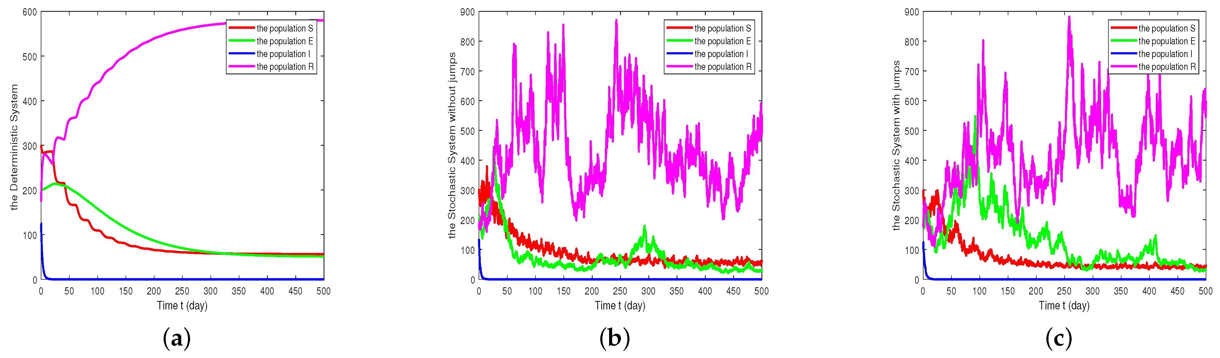
For the assumed parameters, we set $\alpha =0.22,\rho =0.6,\mathbb{Z}=(0,+\infty ),\lambda \left(\mathbb{Z}\right)=1$, the intensity of stochastic disturbance as follows:

$$\begin{array}{c}\hfill {\sigma }_1^2={\sigma }_2^2={\sigma }_4^2=0.01,{\sigma }_3^2=0.02,{\gamma }_1=0.01,{\gamma }_2=0.02,{\gamma }_3=0.08,{\gamma }_4=0.04.\end{array}$$

It is easy to calculate that ${\mathcal{R}}_1\approx 0.9932<1$, and the condition of Theorem 2 is satisfied. The numerical simulation results are given in Figure 1. It can be found that the infected population $I\left(t\right)$ is extinct in both the deterministic model and the stochastic model. In fact, all values of $\beta$ which are less than 0.01498 lead to obtaining a value less than one of the basic reproduction numbers ${\mathcal{R}}_1$ of the system (1), so the disease will always be extinct.

The coefficient $\beta$ can likewise increase if we increase the contact between the infected population and the susceptible population. Similarly, if we reduce the effective vaccination rate among the infected population, the coefficient $\rho$ will decrease. For this analysis, we retain the parameter values used in Table 1, except for $\beta$ and $\rho$, which are chosen to be 0.114 and 0.01, respectively. The values of stochastic noise intensity are as follows:

$$\begin{array}{c}\hfill {\sigma }_1^2=0.003,{\sigma }_2^2={\sigma }_3^2=0.002,{\sigma }_4^2=0.005,{\gamma }_1={\gamma }_3=0.006,{\gamma }_2=0.003,{\gamma }_4=0.008.\end{array}$$

In this case, ${\mathcal{R}}_2\approx 1.2560>1$, satisfying the conditions of Theorem 3, and the numerical simulations are shown in Figure 2. We can find that the trend of persistence in the mean of the infected population $I\left(t\right)$ is consistent with the deterministic model after adding stochastic perturbations. Furthermore, we can calculate $\underset{t\to \infty }{lim\; inf}\langle I\left(t\right)\rangle \ge 0.0973$, which shows the minimum level of infected population in the average sense. By comparing Figure 1 and Figure 2, it becomes evident that the disease contact rate $\beta$ and vaccination rate $\rho$ significantly influence the extinction and persistence of the disease.

Next, we also explore the effect of stochastic disturbance intensity on disease extinction. Parameters $\gamma$ and $\rho$ are set at 0.02 and 0.03, respectively, with other parameter values in Table 1 remain unchanged.

The numerical simulations are presented in Figure 3. When we select the intensities of disturbance are small, such as ${\sigma }_1^2={\sigma }_2^2={\sigma }_4^2=0.01,{\sigma }_3^2=0.02,{\gamma }_1=0.01,{\gamma }_2=0.02$, ${\gamma }_3=0.08,{\gamma }_4=0.04$, it is easy to calculate that ${\mathcal{R}}_1\approx 5.0746>1$, the infected population $I\left(t\right)$ is not extinct in both the deterministic model and stochastic models. When we select larger disturbance intensities, ${\sigma }_1^2={\sigma }_2^2={\sigma }_4^2=0.1,{\sigma }_3^2=0.7$, ${\gamma }_1=0.1,{\gamma }_2=0.2,$${\gamma }_3=0.6,{\gamma }_4=0.4$, it is easy to calculate that ${\mathcal{R}}_1\approx 0.8879<1$, so the condition of Theorem 2 is satisfied. The infected population $I\left(t\right)$ is extinct in the stochastic models with and without jumps (see Figure 3d,e), which indicates that the large intensities of environmental disturbance have a positive effect on the disease extinction. In addition, by comparing Figure 3b,d and Figure 3c,e, we find that the results of stochastic disturbance with jump are consistent with those of stochastic disturbance without jump. Discontinuous environmental shocks described by L$\acute{\mathrm{e}}$vy jumps can also suppress the spread of the disease in our model.

To further analyze the specific effects of different parameters on disease extinction and persistence, parameter sensitivity analysis is as follows:

For disease extinction and persistence, the effects of parameters $\alpha$ and $\beta$ on $I\left(t\right)$ are considered. At the same time, according to the sensitivity analysis formula in reference [38], we obtain

$$\begin{array}{c}\hfill \frac{\partial {\mathcal{R}}_1}{\partial \alpha }·\frac{\alpha }{{\mathcal{R}}_1}=\frac{\alpha }{1+\alpha }>0,\frac{\partial {\mathcal{R}}_2}{\partial \alpha }·\frac{\alpha }{{\mathcal{R}}_2}=\frac{{\left(\alpha ϵ\right)}^{\frac{1}{2}}}{2[{(\mu +{\theta }_2)}^{\frac{1}{2}}+{\left(\alpha ϵ\right)}^{\frac{1}{2}}]}>0,\end{array}$$

(30)

$$\begin{array}{c}\hfill \frac{\partial {\mathcal{R}}_1}{\partial \beta }·\frac{\beta }{{\mathcal{R}}_1}=\frac{\Lambda (1+\alpha )·\beta }{\beta \Lambda (1+\alpha )}=1>0,\frac{\partial {\mathcal{R}}_2}{\partial \beta }·\frac{\beta }{{\mathcal{R}}_2}=\frac{{(\mu +{\theta }_2)}^{\frac{1}{2}}+{\left(\alpha ϵ\right)}^{\frac{1}{2}}}{2[{(\mu +{\theta }_2)}^{\frac{1}{2}}+{\left(\alpha ϵ\right)}^{\frac{1}{2}}]}>0.\end{array}$$

(31)

The results of numerical simulations are shown in Figure 4: (a) select $\alpha =0.22,0.11,$$0.01$, respectively, so we can see that the smaller $\alpha$ is, the faster population $I\left(t\right)$ will go extinct; (b) Select $\alpha =0.22,0.42,0.62$, respectively, so we can see that $I\left(t\right)$ decreases as $\alpha$ decreases; (c) Select $\beta =0.01498,0.014,0.01$, respectively, we can see that the smaller $\beta$ is, the faster population $I\left(t\right)$ will go extinct; and (d) select $\beta =0.114,0.124,0.134$, respectively, so we can see that $I\left(t\right)$ decreases as $\beta$ decreases.

The decrease in parameter $\alpha$ and $\beta$ will lead to the decrease in ${\mathcal{R}}_1,{\mathcal{R}}_2$, and it can be concluded that parameters $\alpha$ and $\beta$ have a positive correlation with the basic reproduction number. That is to say, the closer $\alpha$ is to 0, the better the effect of education on disease infection prevention, as well as the smaller $\beta$ is, and the less contact susceptible people have with infected people, the fewer infected people there are. This indicates that public health education and disease contact rate have a certain role in promoting disease extinction.

For disease extinction and persistence, the effects of parameters $\gamma$ and $\rho$ on $I\left(t\right)$ are also considered. According to the sensitivity analysis formulas, we obtain

$$\begin{array}{c}\hfill \frac{\partial {\mathcal{R}}_1}{\partial \gamma }·\frac{\gamma }{{\mathcal{R}}_1}=-\frac{\gamma }{\gamma +\sigma +\mu +{\theta }_3}<0,\frac{\partial {\mathcal{R}}_2}{\partial \gamma }·\frac{\gamma }{{\mathcal{R}}_2}=-\frac{\gamma }{\gamma +\sigma +\mu +{\theta }_3+2}<0,\end{array}$$

(32)

$$\begin{array}{c}\hfill \frac{\partial {\mathcal{R}}_2}{\partial \rho }·\frac{\rho }{{\mathcal{R}}_2}=-\frac{\rho }{2(ϵ+\mu +\rho +{\theta }_1)}<0.\end{array}$$

(33)

The results of numerical simulations are shown in Figure 5: (a) select $\gamma =0.427,$$0.527,$$0.627$, respectively, so we can see that the smaller $\gamma$ is, the more time the population $I\left(t\right)$ will take to go extinct; (b) select $\gamma =0.427,0.327,0.227$, respectively, we can see that $I\left(t\right)$ increases as $\gamma$ decreases; (c) select $\rho =0.6,0.7,0.8$, respectively, we can see that the smaller $\rho$ is, the more time the population $I\left(t\right)$ will take to go extinct; (d) Select $\rho =0.01,0.02,0.03$, respectively, we can see that $I\left(t\right)$ increases as $\gamma$ decreases.

The decrease in parameters $\gamma$ and $\rho$ will lead to the increase in ${\mathcal{R}}_1,{\mathcal{R}}_2$, and it can be concluded that parameter $\gamma$ and $\rho$ have a negative correlation with the basic reproduction number. In other words, the smaller $\gamma$ is, the fewer the number of infected people will recover, as well as the smaller $\rho$ is, the fewer the number of susceptible people will be vaccinated, such that a greater number of infected people indicates that the disease recovery rate and the vaccination rate have a certain promoting effect on disease extinction.

7. Conclusions

In this paper, we propose a stochastic delayed SEIRS epidemic model considering the impacts of public health education and temporary immunity. We prove the global existence and uniqueness of the positive solution of the system (4), providing sufficient conditions for the extinction and persistence of the disease. We perform numerical simulations to corroborate our results and analyze each parameter’s influence on the disease. In conclusion, factors such as public health education, disease contact rate, disease recovery rate, vaccination rate, and high stochastic noises can all contribute to disease extinction. The higher the levels of education, recovery and vaccination rates, and the level of noise, coupled with a lower rate of contact, the more likely it is for the disease to become extinct. Notably, the basic reproduction numbers ${\mathcal{R}}_1$ and ${\mathcal{R}}_2$ are independent of time delay, suggesting that time delay might not significantly affect the disease’s average persistence and extinction.

The study in reference [5] considered the deterministic susceptible–educated–infective–susceptible (SEIS) model impacted by public health education. The disease extinction threshold ${\mathcal{R}}_0=\beta \Lambda /\left(\mu (\gamma +\sigma +\mu )\right)$ obtained in reference [5] shows a strong relationship between disease extinction and the contact rate, recovery rate, and mortality rate. This paper expands on that by also considering the intensity of stochastic disturbance, thus demonstrating that the average persistence and extinction of infectious diseases are influenced by a combination of these factors. Furthermore, large-intensity noise disturbances can lead to disease extinction, as illustrated in Figure 3. Similarly, both continuous interference described by white Gaussian noise and discontinuous environmental shocks represented by L$\acute{\mathrm{e}}$vy jumps can suppress the spread of the disease in our model.

This work provides a fundamental stochastic delayed dynamical model, which can be instrumental in understanding the impact of public health education and stochastic noises on infectious disease prevention and control. In terms of real-world disease prevention and control efforts, the findings suggest potential measures, such as increasing education awareness, heightening environmental disturbance, minimizing patient contact with others, and encouraging advance vaccination.

References

1. Lu, H. Prevention and Control of Infectious Diseases. Highlights Sci. Eng. Technol. 2023, 36, 871–874. [Google Scholar] [CrossRef]
2. Ghaffar, A.; Rashid, S.F.; Wanyenze, R.K.; Hyder, A.A. Public health education post-COVID-19: A proposal for critical revisions. BMJ Glob. Health 2021, 6, e005669. [Google Scholar] [CrossRef]
3. Eric, P.; Warner, S.B. A potential new front in health communication to encourage vaccination: Health education teachers. Vaccine 2021, 39, 4671–4677. [Google Scholar]
4. Cheng, G.; Wang, N.; Qi, L. Modeling the influence of health education on individual behavior in the process of disease transmission. Math. Methods Appl. Sci. 2022, 45, 498–525. [Google Scholar] [CrossRef]
5. Nyang’inja, R.A.; Angwenyi, D.N.; Musyoka, C.M.; Orwa, T.O. Mathematical modeling of the effects of public health education on tungiasis—A neglected disease with many challenges in endemic communities. Adv. Differ. Equ. 2018, 2018, 426. [Google Scholar] [CrossRef]
6. Buonomo, B.; Carbone, G.; d’Onofrio, A. Effect of seasonality on the dynamics of an imitation-based vaccination model with public health intervention. Math. Biosci. Eng. 2018, 15, 299–321. [Google Scholar]
7. Shi, X.; Gao, X.; Zhou, X.; Li, Y. Analysis of an SQEIAR epidemic model with media coverage and asymptomatic infection. AIMS Math. 2021, 6, 12298–12320. [Google Scholar] [CrossRef]
8. Joshi, H.; Sharma, R.K.; Prajapati, G.L. Stability analysis of a deterministic vaccination model with non-monotonic incidence rate. J. Math. Comput. Sci. 2020, 10, 51–67. [Google Scholar]
9. Fan, K.; Zhang, Y.; Gao, S.; Wei, X. A class of stochastic delayed SIR epidemic models with generalized nonlinear incidence rate and temporary immunity. Phys. A Stat. Mech. Appl. 2017, 481, 198–208. [Google Scholar] [CrossRef]
10. Liu, Y.; Zhang, Y.; Wang, Q. A stochastic SIR epidemic model with Lévy jump and media coverage. Adv. Differ. Equ. 2020, 2020, 70. [Google Scholar] [CrossRef] [Green Version]
11. Kyrychko, Y.N.; Blyuss, K.B. Global properties of a delayed SIR model with temporary immunity and nonlinear incidence rate. Nonlinear Anal. Real World Appl. 2005, 6, 495–507. [Google Scholar] [CrossRef]
12. Xu, R.; Ma, Z.; Wang, Z. Global stability of a delayed SIRS epidemic model with saturation incidence and temporary immunity. Comput. Math. Appl. 2010, 59, 3211–3221. [Google Scholar] [CrossRef] [Green Version]
13. Li, R.; Tian, F.; Hu, X. The stochastic SIV epidemic model with varying coefficient and time delay. Math. Appl. 2016, 29, 890–896. [Google Scholar]
14. Liu, Q.; Jiang, D.; Hayat, T.; Ahmad, B. Analysis of a delayed vaccinated SIR epidemic model with temporary immunity and Lévy jumps. Nonlinear Anal. Hybrid Syst. 2018, 27, 29–43. [Google Scholar] [CrossRef]
15. Hu, Z.; Cheng, X.; Ma, W. Analysis of an SIS epidemic model with temporary immunity and nonlinear incidence rate. Chin. J. Eng. Math. 2009, 26, 407–415. [Google Scholar]
16. Liu, Q.; Chen, Q. Stochastic delayed SIR epidemic with vaccination model and temporary immunity. Sci. Sin. Math. 2016, 46, 1745–1756. [Google Scholar]
17. Shi, X.; Cao, Y.; Zhou, X. Dynamics for a stochastic delayed SIRS epidemic model. Nonlinear Anal. Model. Control. 2020, 25, 705–725. [Google Scholar] [CrossRef]
18. Zhou, X.; Shi, X.; Wei, M. Dynamical behavior and optimal control of a stochastic mathematical model for cholera. Chaos Solitons Fractals 2022, 156, 111854. [Google Scholar] [CrossRef]
19. Shi, X.; Cao, Y. Dynamics of a stochastic periodic SIRS model with time delay. Int. J. Biomath. 2020, 13, 2050072. [Google Scholar] [CrossRef]
20. Zhang, X.; Shao, Y. Analysis of a stochastic predator-prey system with mixed functional responses and Lévy jumps. AIMS Math. 2021, 6, 4404–4427. [Google Scholar] [CrossRef]
21. Fan, C.; Xiong, Z.; Nie, D. Dynamical analysis of a stochastic ratio-dependent predator-prey system with Lévy jumps. Int. J. Appl. Math. Stat. 2014, 52, 169–177. [Google Scholar]
22. Kiouach, D.; El-idrissi, S.E.A.; Sabbar, Y. A novel mathematical analysis and threshold reinforcement of a stochastic dengue epidemic model with Lévy jumps. Commun. Nonlinear Sci. Numer. Simul. 2023, 119, 107092. [Google Scholar] [CrossRef]
23. Liu, Q.; Chen, Q. Analysis of a general stochastic non-autonomous logistic model with delays and Lévy jumps. J. Math. Anal. Appl. 2016, 433, 95–120. [Google Scholar] [CrossRef]
24. Lu, C.; Ding, X. Dynamical behavior of stochastic delay Lotka–Volterra competitive model with general Lévy jumps. Phys. A Stat. Mech. Its Appl. 2019, 531, 121730. [Google Scholar] [CrossRef]
25. Liu, R.; Liu, G. Analysis of a stochastic predator-prey population model with Allee effect and jumps. J. Inequalities Appl. 2019, 2019, 60. [Google Scholar] [CrossRef] [Green Version]
26. Wang, K. Stochastic Biomathematical Models; Science Press: Beijing, China, 2010. (In China) [Google Scholar]
27. David, A. Lévy Processes and Stochastic Calculus; Cambridge University Press: Cambridge, UK, 2004. [Google Scholar]
28. Zhao, Y.; Yuan, S. Stability in distribution of a stochastic hybrid competitive Lotka–Volterra model with Lévy jumps. Chaos Solitons Fractals 2016, 85, 98–109. [Google Scholar] [CrossRef]
29. Liptser, R.S. A strong law of large numbers for local martingales. Stochastics 1980, 3, 217–228. [Google Scholar] [CrossRef]
30. Liu, Q.; Chen, Q.; Jiang, D. The threshold of a stochastic delayed SIR epidemic model with temporary immunity. Phys. A Stat. Mech. Its Appl. 2016, 450, 115–125. [Google Scholar] [CrossRef]
31. Ehrenberg, J.P.; Ault, S.K. Neglected diseases of neglected populations: Thinking to reshape the determinants of health in Latin America and the Caribbean. BMC Public Health 2005, 5, 119. [Google Scholar] [CrossRef] [Green Version]
32. Higham, D.J. An algorithmic introduction to numerical simulation of stochastic differential equations. SIAM Rev. 2001, 43, 525–546. [Google Scholar] [CrossRef]
33. Protter, P.; Talay, D. The Euler scheme for Lévy driven stochastic differential equations. Ann. Probab. 1997, 25, 393–423. [Google Scholar] [CrossRef]
34. Mussa, M.; Vivian, M.; Valeria, S.; Hoseenu, P.; Winfrida, J.; Eliud, Y.Y.; Donath, T. Tungiasis infection among primary school children in Northeastern Tanzania: Prevalence, intensity, clinical aspects and associated factors. IJID Reg. 2023, 7, 116–123. [Google Scholar]
35. CIA. The CIA World Factbook; Skyhorse Publishing: New York, NY, USA, 2011. [Google Scholar]
36. IndexMundi. Kenya Demographic Profile. 2018. Available online: https://www.indexmundi.com/kenya/demographics_profile.html (accessed on 18 September 2021).
37. Kong, L.; Li, L.; Kang, S.; Liu, Y.; Feng, W. Dynamic Behavior of a Stochastic Tungiasis Model for Public Health Education. Discret. Dyn. Nat. Soc. 2022, 2022, 4927261. [Google Scholar] [CrossRef]
38. Samsuzzoha, M.; Singh, M.; Lucy, D. Uncertainty and sensitivity analysis of the basic reproduction number of a vaccinated epidemic model of influenza. Appl. Math. Model. 2013, 37, 903–915. [Google Scholar] [CrossRef]
Figure 1. Numerical simulations of the SEIRS deterministic model and stochastic model of disease extinction, where (a) is the deterministic model and (b) is the stochastic model without jumps and (c) is the stochastic model with jumps.
Axioms 12 00560 g001
Figure 2. Numerical simulations of the SEIRS deterministic model and stochastic model of disease are persistent, where (a) is the deterministic model, and (b) is the stochastic model without jumps and (c) is the stochastic model with jumps.
Axioms 12 00560 g002
Figure 3. Numerical simulations of the SEIRS deterministic model and stochastic model of disease extinction, where (a) is the deterministic models, (b,d) are the stochastic models without jumps and (c,e) are the stochastic models with jumps. Here, the disturbance intensity parameters in (b) are σ 1 2 = σ 2 2 = σ 4 2 = 0.01 , σ 3 2 = 0.02 , in (c) are σ 1 2 = σ 2 2 = σ 4 2 = 0.01 , σ 3 2 = 0.02 , γ 1 = 0.01 , γ 2 = 0.02 , γ 3 = 0.08 , γ 4 = 0.04 , in (d) is σ 1 2 = σ 2 2 = σ 4 2 = 0.1 , σ 3 2 = 0.7 , and in (e) are σ 1 2 = σ 2 2 = σ 4 2 = 0.1 , σ 3 2 = 0.7 , γ 1 = 0.1 , γ 2 = 0.2 , γ 3 = 0.6 , γ 4 = 0.4 .
Axioms 12 00560 g003
Figure 4. Numerical simulations of the population I ( t ) of disease extinction and persistence under different parameter α and β , where (a) is disease extinction of α , and (b) is disease persistence of α ; (c) is the disease extinction of β ; and (d) is the disease persistence of β .
Axioms 12 00560 g004
Figure 5. Numerical simulations of the population I ( t ) of disease extinction and persistence under different parameters γ and ρ , where (a) is disease extinction of γ , and (b) is disease persistence of γ , (c) is disease extinction of ρ , and (d) is the disease persistence of ρ .
Axioms 12 00560 g005