
Noninteger Dimension of Seasonal Land Surface Temperature (LST)
1
Department of Urban Planning and Design, Shiraz University, Shiraz 71345, Iran
2
Department of Mechanical Engineering, Florida State University, Tallahassee, FL 32306, USA
*
Author to whom correspondence should be addressed.
Axioms 2023, 12(6), 607; https://doi.org/10.3390/axioms12060607
Submission received: 14 April 2023
/
Revised: 5 June 2023
/
Accepted: 14 June 2023
/
Published: 19 June 2023
(This article belongs to the Section Geometry and Topology)
Abstract
:During the few last years, climate change, including global warming, which is attributed to human activities, and its long-term adverse effects on the planet’s functions have been identified as the most challenging discussion topics and have provoked significant concern and effort to find possible solutions. Since the warmth arising from the Earth’s landscapes affects the world’s weather and climate patterns, we decided to study the changes in Land Surface Temperature (LST) patterns in different seasons through nonlinear methods. Here, we particularly wanted to estimate the noninteger dimension and fractal structure of the Land Surface Temperature. For this study, the LST data were obtained during the daytime by a Moderate Resolution Imaging Spectroradiometer (MODIS) on NASA’s Terra satellite. Depending on the time of the year data were collected, temperatures changed in different ranges. Since equatorial regions remain warm, and Antarctica and Greenland remain cold, and also because altitude affects temperature, we selected Riley County in the US state of Kansas, which does not belong to any of these location types, and we observed the seasonal changes in temperature in this county. According to our fractal analysis, the fractal dimension may provide a complexity index to characterize different LST datasets. The multifractal analysis confirmed that the LST data may define a self-organizing system that produces fractal patterns in the structure of data. Thus, the LST data may not only have a wide range of fractal dimensions, but also they are fractal. The results of the present study show that the Land Surface Temperature (LST) belongs to the class of fractal processes with a noninteger dimension. Moreover, self-organized behavior governing the structure of LST data may provide an underlying principle that might be a general outcome of human activities and may shape the Earth’s surface temperature. We explicitly acknowledge the important role of fractal geometry when analyzing and tracing settlement patterns and urbanization dynamics at various scales toward purposeful planning in the development of human settlement patterns.
1. Introduction
With increasing temperatures around the world, photosynthesis and microbial and plant respiration and, as a result, the release of carbon dioxide to the atmosphere also increase [1]. During recent decades, climate change and its long-term impacts, such as accelerating ice melt in poles, warming oceans, and the rising sea level, as well as influences on many other aspects of life throughout the Earth, have been widely recognized by many different organizations and researchers [2,3]. According to the most recent Intergovernmental Panel on Climate Change (IPCC) report (IPCC, 2014 [4]), greenhouse gases (GHG) are at the highest level, causing the most significant changes in the Earth’s temperature in history [3]. Human activities have significantly increased the concentration of greenhouse gases in the atmosphere and caused global warming, which is adversely affecting all life on the Earth [4,5]. Climate change and global warming result from human activities that change the Land Surface Temperature (LST), causing significant changes to the ecosystem’s structure and, consequently, function [6,7]. For example, they caused an acceleration in environmental status changes on the Tibetan Plateau (Zhong et al. (2011)) [7]. Many studies have also documented the effects of land-use and land-cover change, which are caused by human activities involving land–atmosphere interactions (Boisier et al., 2013, Boisier et al., 2012, de Noblet-Ducoudré et al., 2012) [8,9,10].
States at Risk, which is a project undertaken to demonstrate the effects of climate change in all 50 states of the United States, divides climate changes impacts into five categories: extreme heat, drought, wildfires, coastal flooding, and inland flooding. There are many real-world examples of these five impacts of climate change in different parts of the Earth. For example, the devastating bush fires that happened in Australia in 2019 because of high temperatures are one the most dramatic recent disasters resulting from climate change, which followed extreme heat and a long drought and killed people and animals (Source(s): SafeHome.org, States at Risk). Across the United States, we can see different impacts of climate change in daily life, such as extreme heat during summer and intolerable cold during winter, destructive storms, wildfires and prolonged bush fires on the plains, and many other events that have significant impacts on the economy and other aspects of life. Since vegetation significantly affects the Land Surface Temperature (LST) distribution, there have been studies to evaluate the LST–vegetation relationship [11]. Kumar et al., 2015 also calculated the occurrence of the vegetation parameter, which determines the distribution of the LST. If we compute the distribution of the Land Surface Temperature (LST) and its spatial variation, then we can understand the mechanism underlying the air temperature increase in urban areas [11].
The Land Surface Temperature (LST) plays a key role in environmental studies and climate research [3]. The LST demonstrates the temperature of any surface of the Earth in a specific location. Since, a MODIS satellite collects the data through the atmosphere to the ground, this surface can be snow, ice, grass, leaves of trees, or roofs of buildings. Therefore, the LST is not the same as the air temperature that we hear about in the daily weather report. The LST is a combination of vegetation and bare soil temperatures, and because these two factors can change quickly in response to any solar radiation or aerosol variation, the LST demonstrates rapid changes as well. Scientists, by collecting these data, want to find the relationship between increasing atmospheric greenhouse gases and the Land Surface Temperature, and generally speaking, discover the impact of an increasing LST on glaciers, ice sheets, permafrost, and the vegetation in the Earth’s ecosystems (Source(s): Moderate Resolution Imaging Spectroradiometer (MODIS)). Recently, it has been shown that the Land Surface Temperature (LST) data collected using Moderate Resolution Imaging Spectroradiometer (MODIS) from both the Terra and Aqua platforms can be applied for linear regression models of daily air temperatures at the local scale [12]. Land Surface Models (LSMs) have been used to estimate the water content, vegetation, and soil temperature [13]. These models take meteorological data, such as the air temperature, humidity, pressure, and other input data, and estimate soil evaporation and plant transpiration as outputs [14,15]. In general, these models are based on the mass transfer (MT) equation and the Penman–Monteith (PM) equation, which are two common frameworks used in land surface modeling for the purpose of evapotranspiration (ET). It has been shown that evapotranspiration (ET) estimation using the Penman–Monteith (PM) equation provides more reliable results compared to when we use the mass transfer (MT) equation [14].
In the United States, southwest areas, including the central plains in Kansas, are faced with unprecedented droughts. Increasing the Earth’s temperatures and reducing rainfall will cause more extreme droughts in the future, adversely affecting the urban dwellers and also farmers across this state. Using the data published by Climate Central (an independent organization with the purpose of conducting research about the climate change and its impact on the public), the state of Kansas has been faced with extreme heat, drought, wildfires, and inland flooding resulting from global warming (Source(s): Climate Central, SafeHome.org, States at Risk). In Figure 1, we can see the seasonal changes in the Land Surface Temperature (LST) in Riley County in the US state of Kansas obtained via the Google Earth Engine for winter 2021–winter 2022.
Climate is a complex system since not all the variables in this system can be observed, and because of uncertainty, our ability to predict is limited. To describe complex natural processes, in 1983, Benoit Mandelbrot introduced fractals as immensely useful objects in numerous scientific fields [16]. Mathematically speaking, fractals are infinitely irregular self-similar objects that are characterized by power law or a scaling exponent over a wide range of scales [16,17]. Thanks to Mandelbrot’s research in fractal geometry, Earth scientists are able to determine probabilities and predict the size, location, and timing of future natural disasters by measuring past events. If a certain process can be characterized by a single scaling exponent, then it is called monofractal. However, if a phenomenon requires a large number of scaling exponents (can be infinite) to characterize its scaling structure, then it is called multifractal [18,19,20]. Euclidean geometry can be used to explore regular patterns; however, a wide range of irregular patterns exist in real-world data, which may need to be described based on their heterogeneity and self-similarity using fractal geometry. Self-similarity is the main property of fractal patterns that are repeated at different scales. The fractal dimension has been used frequently to measure the degree of self-similarity and complexity of a fractal object. If we measure the Hausdorf–Besicovitch dimension of a fractal object, it exceeds the topological dimension and may vary between one and two. Here, one means a process that can be a time series in which data are completely differentiable, and two refers to an irregular object that takes up the entire two-dimensional topological space. Therefore, when we classify data based on their fractal geometry, it is important to examine the complexity index of data to understand whether our data demonstrate some evidence of variation across different scales. P. A. Burrough conducted a study on different environmental data and concluded that they follow fractal patterns and they have a wide range of fractal dimensions [21]. In studying real-world time series data, we may deal with databases that exhibit the power law or self-similarity over a wide range of size and time scales. For this type of phenomenon, we need to apply nonlinear techniques to characterize the complexity and self-similarity of data, because the traditional time series techniques fail to classify databases with a variety range of scaling features [2,22,23,24,25,26]. In this study, for the first time, we aim to determine whether the Land Surface Temperature (LST) may also exemplify some general principles of systems with self-organization patterns. A properly designed study could also be applied to other areas around the world to obtain a big picture of urban developmental trajectories and their impacts on the Earth’s surface temperature. Thus, we propose that a fractal geometry framework may provide a rigorous analytical technique to analyze and model settlement patterns in Riley County in the US state of Kansas which can be extended to different parts of the world.
The present study investigates the self-similarity and power law structures of the Land Surface Temperature (LST) time series data using some nonlinear techniques and fractal geometry. We start with a statistical regression analysis on the Land Surface Temperature (LST) databases of a selected region, Riley County in the US state of Kansas. This database was constructed using Google Earth Engine and the Moderate Resolution Imaging Spectroradiometer (MODIS) on NASA’s Terra satellite. Because of the irregularity in the nature of the LST database on different days of the year, we used nonlinear methods, such as power law analysis, fractal dimension analysis, and the multifractal spectrum technique to characterize the structure of data. A vibration analysis using the power spectral density (PSD) method was performed to determine whether some type of power law scaling exists for various statistical moments at different scales of these databases. Then, we used the Discrete Wavelet Transform (DWT) and Wavelet Leader Multifractal (WLM) analyses to identify the possibility of these time series databases belonging to the class of multifractal process for which a large number of scaling exponents are required to characterize their scaling structures. Finally, a nonlinear analysis called the Fractal Dimension (FD) analysis using the Higuchi algorithm was carried out to quantify the fractal complexity of the data.
2. Materials, Methods, and Results
2.1. Data: The Land Surface Temperature (LST) of Riley County for February, April, July, and October (2021)
By using Google Earth Engine (GEE), we can obtain the MODIS (Moderate Resolution Imaging Spectroradiometer) Terra LST data using the “MODIS/006/MOD11A1” image collection which provides eight-day composite LST images at a 1 km spatial resolution. MODIS has global coverage and provides monitoring LST values over large areas. GEE performs a built-in atmospheric correction algorithm which is called the “Split Window Algorithm” for the MODIS Terra LST product. Using this algorithm, the LST values in two thermal infrared bands (band 31 and band 32) may be corrected to account for atmospheric effects. By default, GEE involves land-cover-specific emissivity values for the atmospheric correction process. Then, the emissivity values may be utilized to correct the variations in surface emissivity and improve the accuracy of LST estimates. Moreover, by using GEE we are able to compare LST data collected from different satellites, such as Landsat and Sentinel-2.
The study area was Riley County, which is located in the US state of Kansas. According to the US Census Bureau, its total area is 622 square miles (1610 km), including 610 square miles (1600 km) of land and 12 square miles (31 km) () of water (Source(s): US Gazetteer files: 2010, 2000, and 1990. United States Census Bureau. 12 February 2011. Retrieved 23 April 2011). The present study investigated the nonlinear patterns of daytime (LST) databases that were collected using Google Earth Engine (GEE) and over Riley County in the US state of Kansas. Google Earth Engine is a combination of a multipetabyte catalog of satellite imagery and geospatial databases with planetary-scale analysis capabilities [27]. GEE helps to track changes and/or measure differences on the Earth’s surface and has been used widely to find map trends. LST databases include remotely sensed data taken from MODerate Resolution Imaging Spectroradiometer (MODIS) sensor in the form of 16-day composites of daytime values at a resolution of 1 km during February, April, July, and October (2021) (see Figure 2 and Figure 3).
In the present study, we were interested in classifying LST data and visualizing their pattern using nonlinear techniques in fractal geometry (see Figure 4). We took advantage of MODIS to display the global climate patterns in land surface dynamics, which was useful to understand changes in temperature across different regions. MODIS has been used since 2000 and provides a long-term data record that is a comprehensive source for learning more about the long-term trends in LST and its impact on climate changes. In addition, this valuable historical data resource helps us to analyze interannual alterations and extract long-term climate trends and can be obtained from the public resource (accessed on 21 October 2021 https://search.earthdata.nasa.gov/).
2.1.1. Time Series Regression Analysis
To explore and quantify the trends and patterns in the LST database, we performed a time series regression analysis. Time series regression is a statistical technique that uses experimental data to predict the future LST based on the current LST responses by transferring the dynamics of our predictor, which is the height. This forecasting method provides a great understanding of the structure of the dynamic system which is the LST database [28].
We started by defining the design matrix of current and past height data ordered by time, and we called this matrix a regressor matrix. Next, we used the ordinary least-squares (OLS) method for the linear regression (LR) equation:
where is the linear estimator parameter, and represents the LST database. The model (1) helped us to find the linearity between the LST variable and the regressor matrix .
2.1.2. Time–Frequency Analysis Using Continuous Wavelet Transform (CWT) and Wavelet-Based Semblance Analysis
When we are working with stationary databases with constant frequencies throughout the time intervals of data, the Fourier transform helps to visualize the data over time; however, this technique fails when we have datasets that are changing over time in response to a particular stimulus, i.e., they have time-varying features [29,30]. This is the main limitation of the Fourier transform, which gives a broad power spectrum by integrating the frequency of time series data across the whole dataset. Because our Day LST databases are nonstationary, we applied time–frequency methods, such as the Continuous Wavelet Transform (CWT). Wavelet-based approaches provide the ability to account for temporal (or spatial) variability in spectral character. Although wavelet analysis is relatively new compared with Fourier analysis, its use has become widespread in recent years, and so the theory is described only briefly here [31]. Mallat (1998) or Strang and Nguyen (1996) contain excellent and detailed summaries of wavelet analysis. The continuous wavelet transform (CWT) of a dataset h(t) is given by (Mallat, 1998) [31,32]
where s is the scale, u is the displacement, is the mother wavelet used, and * means a complex conjugate. The CWT is, therefore, a convolution of the data with the scaled version of the mother wavelet. Of course, the time coordinate t in Equation (3) can also be a spatial coordinate x if profile data are being analyzed. We display the time frequency of the Land Surface Temperature (LST) in Riley County during February, April, July, and October (2021) in Figure 6.
Similarity measures are becoming increasingly used in comparisons of multiple datasets from various sources. Semblance filtering compares two datasets on the basis of their phase as a function of frequency. For semblance analysis based on the Fourier transform [33]
where is dataset, f represents the frequency, and t is the time, there are problems associated with the transform, in particular, its assumption that the frequency content of the data must not change with time (for time series data) or location (for data measured as a function of position). To overcome these problems, semblance is calculated here using the continuous wavelet transform. When calculated in this way, semblance analysis allows the local phase relationships between the two datasets to be studied as a function of both scale (or wavelength) and time [31,34].
When we define the Fourier transform (4) of time series datasets and , the semblance S or the difference in the phase angle at each frequency can be obtained using the following formula [35,36]:
where and represent the real parts of the Fourier transform of dataset 1 and dataset 2, respectively; and demonstrate the imaginary parts of the Fourier transform of dataset 1 and dataset 2, respectively; and the semblance S varies from to . If , a perfect phase correlation exists; for , there is no correlation; and for , we have a perfect anticorrelation. However, the the Fourier-based semblance method (5) does not work well in real-world applications, as it fails to present the correlations in time series data. Therefore, for our study to find the correlation between two time series of data, we used a wavelet-based method called the cross-wavelet transform, which was introduced by (Torrence et al. (1998)) and has the form [34]:
This is a complex quantity and its amplitude, which is called the cross-wavelet power, is defined as
with the local phase
The local phase measures the phase correlation between two time series of data. Now, we define the wavelet-based semblance as the form
Here, is an odd integer. For , our time series datasets are inversely correlated; for , they are uncorrelated; and for , they are correlated. However, the wavelet-based semblance (8) fails to demonstrate the correlation between two noisy time series of data because of the lack of amplitude information [31]. Therefore, we defined the vector dot product of the two complex wavelet vectors at each point in terms of the scale and position as [31]
As we can see from Equation (9), D is a combination of the wavelet-based semblance (8) and the cross-wavelet power (7), which helps us to find the phase correlations of the larger amplitude components of the noisy dataset.
In Figure 7, we plot the dot product D of the Land Surface Temperature (LST) for Riley County (Figure 3) during February, April, July, and October (2021) using Formula (9) where dark red corresponds to large-amplitude signals with a semblance of +1, and yellow corresponds to large-amplitude signals with a positive semblance between 0 and +1. The semblance results show that the LST dataset and height dataset are highly correlated.
2.1.3. Vibration Frequency Analysis via the Power Spectral Density (PSD)
Power spectral density (PSD) analysis is one of the methods used in frequency-domain analyses that has been used frequently to analyze signal vibrations. Power defines the magnitude of the PSD, which is the mean square value of the given time series data. PSD, as a function of frequency, demonstrates the distribution of time series data over a spectrum of frequencies, and its magnitude is normalized to a single Hertz bandwidth. PSD curves display the continuous probability density function of each measure, and they are obtained by multiplying each frequency bin of the fast Fourier transform (FFT) by its complex conjugate to obtain a real spectrum. Because the nature of the LST database is nonlinear and nonstationary, the Welch (PSD) method with overlapped segmentation, which is an averaging estimator technique, was applied to study the complex fluctuations in LST structures. Then, we used the least square approximation technique to fit a linear regression model to the logarithm of the power spectral density of the LST database. Finally, we computed the slope for each regression model of LST data. In Figure 8, we show the fitted least-squares approximation to the logarithm of the power spectral density of the Land Surface Temperature (LST) of Riley County during February, April, July, and October (2021).
In fractal processes, we can find a scaling relationship between power and frequency f in the spectral domain. The PSD results in Figure 8 represent the fractal structure in the LST database via a linear, negative slope of fitted least square lines. As a result, the LST time series data cannot be obtained by one or a finite set of subsystems, and different components in each fractal process act at different time scales. Even though the PSD revealed the power law structure in LST databases, it failed to classify these four groups of data.
2.2. Fractal Geometry and the World’s Weather and Climate Patterns
2.2.1. Multifractal Analysis and the Discrete Wavelet Transform (DWT)
We have shown that complex structures in LST databases, presented in Figure 3, exhibit long-range correlations, i.e., they are self-similar. Statistically, vibrations on one time scale are similar to those at multiple other time scales. To discover whether these four groups of LST data belong to the class of multifractal processes or whether they are monofractal, we plotted the scaling exponents of the Land Surface Temperature (LST) in Riley County during February, April, July, and October (2021) in Figure 9.
The nonlinear relationships between scaling exponents and the statistical moments could be a sign of multifractality in the structure of data; however, we need to check this claim via multifractal analysis. Multifractal analysis helps us to understand whether the LST databases are multifractal, i.e., a larger number of scaling exponents is required to characterize the scaling structures of time series data. To investigate the scaling law of a multifractal process, the standard partition multifractal function was first introduced, which was based on the generalized fluctuation analysis. However, it failed to fully characterize the scaling behavior of the nonstationary time series data [37]. Arneodo et al., 1995b [38], and Bacry et al., 1993 [39], Muzy et al., 1993, 1994 [40] developed statistical techniques based on the Continuous Wavelet Transform (CWT) to characterize the multifractal description of singular measures. Arneodo et al., 2002 developed a method called the Wavelet Transform Modulus Maxima (WTMM) to solve the deficiency of the partition multifractal function and provided wide insight into a variety of problems. Abry et al., 2000, 2002a,b [41,42,43] and Veitch and Abry, 1999 [44] developed a multifractal analysis based on the Discrete Wavelet Transform (DWT) including the recent use of Wavelet Leaders (WLs) (Jaffard et al., 2006 [45], Wendt and Abry, 2007 [46], Wendt et al., 2007 [47]). In this study, we focused on the multifractal analysis using DWT and WLs [45,46,47,48,49,50,51]. The wavelet analysis associates the dimension of the fractal sets with the Hölder exponent to quantify the spectrum of singularity of the pointwise regular function F [45]. The Hölder exponent of a fractal process can be defined as follows:
Definition 1
([51]). A fractal process satisfies a Hölder condition, when exists, such that
We can find for a constant F from the coarse Hölder exponents as
The following sets may be defined to extract the geometry of a signal
with varying d. These sets describe the local regularity of a signal. We call the map
which is a compact form of the singularity structure of the fractal process F, the multifractal spectrum of F [51]. In a global setting, to describe the complexity of a signal, we may need to count the intervals over which the fractal process F evolves with the Hölder exponent and give an estimation of . The grain exponent, which is a discrete approximation to , can be written in the following form [51]
Therefore, the grain multifractal spectrum has the form [48,49,50]
where
From the multifractal analysis presented in Figure 10, we can easily see a clear loss of multifractality in all four groups of (LST) time series data, i.e., they are homogeneous and monofractal, since their spectrum displays a scaling exponent of narrow width.
2.2.2. Higuchi Fractal Dimension Algorithm
One of the key concepts in the theory of fractal geometry is the concept of the fractal dimension. There are a variety of techniques to approximate the dimensions of an irregular object. For example, the dimensions of an object can be obtained by covering it with small boxes. The Hausdorff–Besicovitch dimension, or box-counting dimension, is one of the most frequently used methods to estimate the fractal dimension, which works in this way [52]. To find the box-counting dimension, we consider a square and partition it into grids of linear length . If defines the total number of boxes, then the total measure will be [53]:
where we denote the measuring unit by and try out a number of different values. If we choose , then as . This means that the length of a square is infinite, which makes sense. If we try , then as . This means that the volume of a square is 0, which is also correct. For , we can find the true dimensions of the square. Using this argument, we define the Hausdorff–Besicovitch dimension as follows: First, we need the -covering measure, which is the summation of the total measure in all “boxes” denoted by , , subject to the condition that the union of the boxes covers the object E, while the size of the largest is not greater than :
Using (18), can be defined by
Although this method can successfully measure the self-similarity of a fractal process, it fails when sudden changes happen in irregular time series datasets [54]. To solve this problem, a variety of different nonlinear methods, such as the Higuchi algorithm, power spectrum analysis, and Katz algorithm have been developed by different researchers [55,56]. To find the fractal dimension of each LST time series of data, we applied the Higuchi Algorithm [55]. At first, we defined a finite time series
and we created k new time series of the form
such that . For each time interval k and the initial time , we computed the length of via
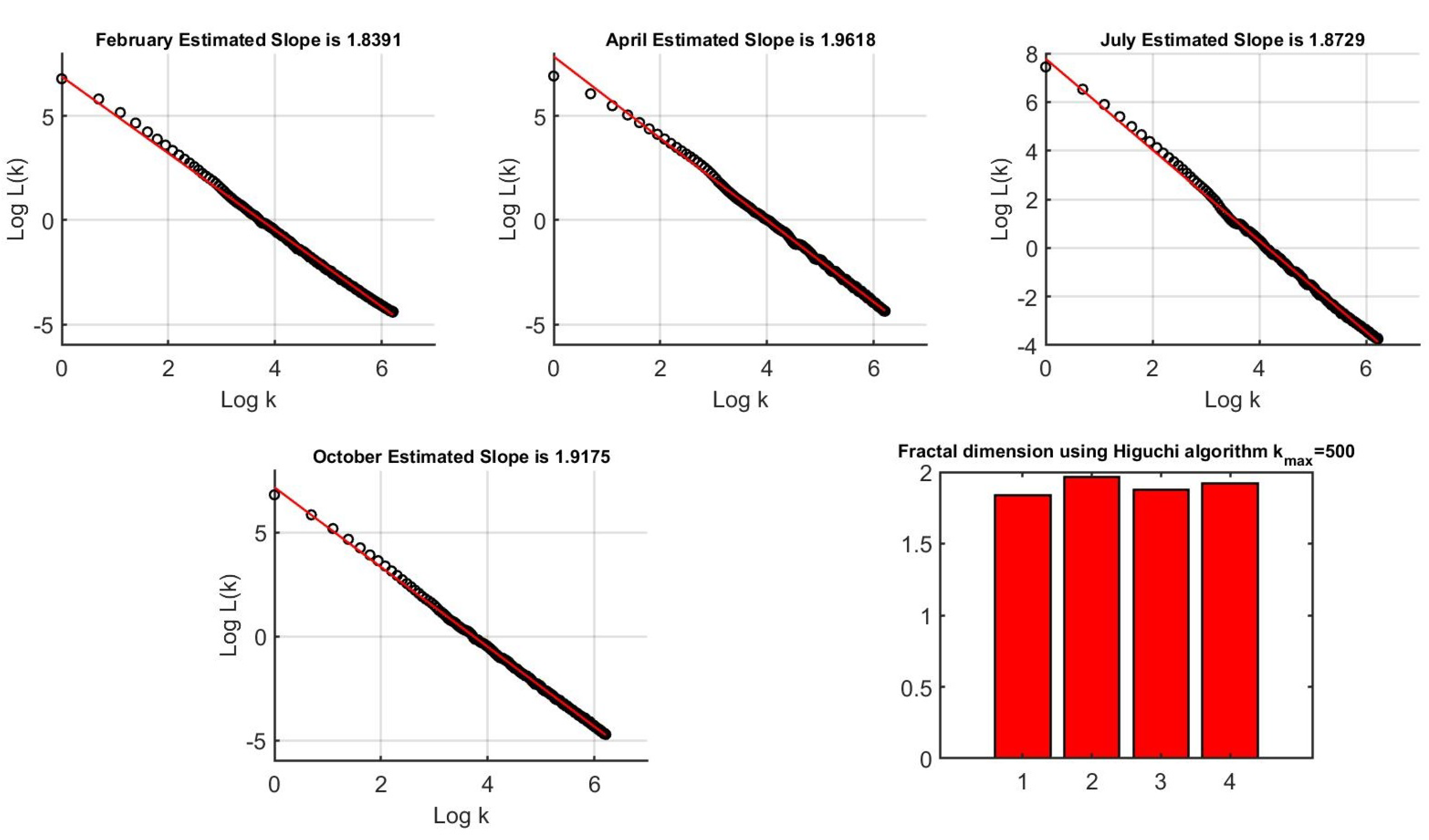
where is called the curve length normalization factor. Next, we calculated the mean of for to find the average curve length for each . Then, we plotted versus for different time intervals k. Finally, we used the least-squares approximation to estimate the slope of each regressed line as the Higuchi fractal dimension for an optimal time interval of (optimal means there is no change in the Higuchi fractal dimension after this value).
We estimated the fractal dimension of the Land Surface Temperature (LST) for Riley County during February, April, July, and October (2021) and plotted their regression models for each time series in Figure 11.
From the results in Figure 11, we can compare the fractal dimensions of different LST data, as follows:
Although the fractal dimension using the Higuchi algorithm is a good index for comparing the self-similarity and complexity in the fractal structures of different (LST) datasets, it fails to classify four groups of LST datasets and we need to extend our study to a larger dataset to obtain a complexity index that can be used to classify different LST data.
3. Discussion
During recent decades, the rapid modification of the land’s surface by human activities has caused numerous environmental impacts. Land surface plays an important role in the structure of the climate system, and many related organizations have put significant effort into the building of observational land surface systems. Since controlling the Land Surface Temperature (LST) strongly impacts the climate change at the local and global scales, we decided to analyze the complexity of the LST database to better understand its pattern and structure. In [21], P. A. Burrough showed that environmental data are fractals and may satisfy a wide range of fractal dimensions. Although there are many different approaches to the modeling of the Land Surface Temperature based on the mass transfer (MT) equation and the Penman–Monteith (PM) equation, they need some improvements to allow the capture of the seasonal variation of parameters and the quantification of spatial heterogeneity. Some of the main disadvantages of these models are as follows: (1) the MT equation is less robust compared to the PM equation for land surface models (LSMs), (2) evapotranspiration (ET) estimated using the MT equation faces huge uncertainty in warm and wet seasons, while evapotranspiration (ET) estimated using the PM equation demonstrates better results than the eddy covariance (EC) technique [14].
In the present study, we combined the theory of fractal geometry with the Land Surface Temperature (LST) to construct a fractal model and fit it to real-world LST data. We used satellite data from the Moderate Resolution Imaging Spectroradiometer (MODIS) for the Land Surface Temperature (LST) in Riley County during February, April, July, and October (2021), and we conducted our research within the framework of fractal geometry. To explore the differences in the fractal patterns and complex dynamics of different (LST) datasets, we established our analysis based on different quantitative and analytical nonlinear methods to find a computational framework for the classification of (LST) databases. We started with a vibration analysis using the power spectral density (PSD) method to estimate the exponent from realizations of these processes and to find out whether the data of interest exhibit a power law PSD. We performed a multifractal analysis using discrete wavelet methods to discover whether some type of power law scaling exists for various statistical moments at different scales of LST databases and also to explore whether our database follows a multifractal structure for which a large number of scaling exponents is required to characterize scaling structures. Finally, we computed the Higuchi fractal dimension of LST databases for each group to compare the complexity of LST databases in different time intervals. We were also interested to simply test weather the simple linear regression model will be a good candidate to model the the Land Surface Temperature (LST) data and the results are represented in Appendix A.
This study revealed that the (LST) databases are monofractal, i.e., their spectrum displays a narrow width for the scaling exponent. In another word, a single global exponent is enough to characterize the fractal behavior and scaling properties of time series data. This also indicates that the LST data show the same statistical properties at different scales or follow scale invariance properties. Using the fractal dimension, we recognized the natural complexity in the structure of the LST data. Fractal analysis could help to improve our knowledge of the Land Surface Temperature and to reveal some of the underlying mechanisms of the warmth rising off the Earth’s landscapes, which affects climate patterns and the world’s weather. By monitoring the altered complexity in the structure of LST data, we can characterize how the Land Surface Temperature patterns vary throughout the year.
To date, no research exists on the use of fractal geometry to classify Land Surface Temperature (LST) data, and since LST data play a key function in the physics of land surface processes from local through to global scales [57], it is crucial to apply appropriate techniques that are able to model underlying LST patterns and structures. We applied the main property of a fractal, which is self-similarity across different spatial scales or resolutions of observation, to describe the altered geometrical structure of LST data. Our proposed fractal model is robust and may capture a multiscale birth–death process in the structure of LST data obtained from power law and self-organized patterns. In the present study, we successfully modeled LST distribution patterns, which are sources of heterogeneity and complex space–time structures. This important and novel finding helps us to better understand the structure of LST databases and, consequently, better control climate change caused by human activities. However, because of the limited number of databases, vibration analysis using PSD, the fractal dimension, and multifractal analysis alone may not be sufficient to classify LST databases for different seasons; however, they may be used as a comprehensive framework to further analyze, characterize, and compare the fractal behavior of LST time series and extract their complex structures. A future direction for this study would be to utilize more databases from different climates, time scales, and locations to support our conclusion.
Our study has some limitations that must be addressed. One limitation is the sample size as our data were limited to a specific region and time of the year. Although fractal geometry may be an effective method to describe and predict environmental patterns at multiple scales, more studies need to be performed using larger data sizes to be able to introduce the fractal dimension as a useful index to classify environmental data. The use of more LST values and the collection of broad and diverse samples would resolve this restriction. It must be noted that no environmental pattern can truly follow a fractal model. We also stress that more analyses need to be performed to describe the heterogeneity and local properties of environmental data and, strictly speaking, to find the lower and upper bounds of the fractal dimension.
Author Contributions
Conceptualization, S.A. and T.A.; methodology, S.A. and T.A.; software, S.A. and T.A.; validation, S.A. and T.A.; formal analysis, S.A. and T.A.; investigation, S.A.; resources, S.A.; data curation, S.A.; writing—original draft preparation, S.A.; writing—review and editing, S.A.; visualization, S.A.; supervision, T.A.; project administration, T.A.; funding acquisition, T.A. All authors have read and agreed to the published version of the manuscript.
Funding
This research received no external funding.
Data Availability Statement
Suggested Data Availability Statements are available at https://earthobservatory.nasa.gov/global-maps/MOD_LSTD_M accessed on 12 April 2023.
Conflicts of Interest
The authors declare no conflict of interest.
Appendix A. Traditional Statistical Analysis
In this study, we applied the time series linear regression to find the linear relationship between the LST variable and the regressor matrix in model (1) using the Land Surface Temperature (LST) data in Figure 3. Due to simplicity, the linear regression analysis is useful to better understand the relationships among variables and or to model multiple independent variables. Consequently, it can be applied in the decision-making process regarding environmental issues to make appropriate policies. In Figure A1, we can see the time series linear regression analysis of the seasonal LST in Riley County during February, April, July, and October (2021) obtained via Google Earth Engine in Figure 3.
Here, we analyze the time series linear regression in Figure A1 to test whether the linear model works well for the Land Surface Temperature (LST) data or not. At first, we check whether the residuals have nonlinear patterns or not. We plotted the residuals vs. fitted graph for February, April, July, and October (2021) Figure 3 in Figure A2, Figure A3, Figure A4 and Figure A5, separately. According to the residuals vs. fitted results, we have almost equally spread residuals around the horizontal line (no distinct patterns), which means that there are no nonlinear relationships in any of the time series regression models.
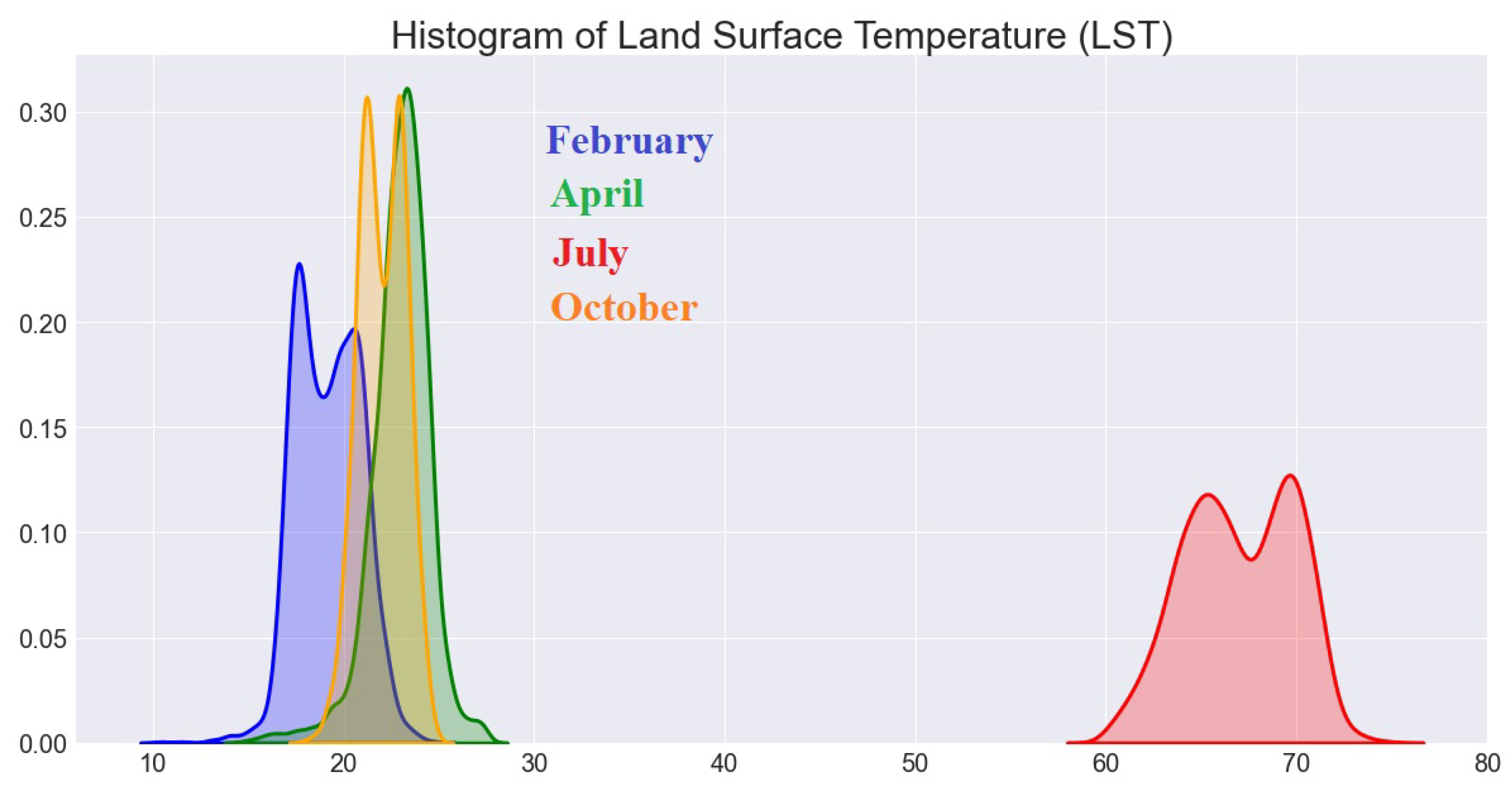
Secondly, we are interested in checking whether residuals are normally distributed. Therefore, we plotted normal quantile–quantile (Q-Q) graphs of the Land Surface Temperature (LST) data (Figure 3) in Figure A2, Figure A3, Figure A4 and Figure A5, separately. In fact, Q-Q plots are scatter plots that are produced when we plot a set quantile against another one. As we can see from the Q-Q plots, residuals do not follow a straight line very well and they deviate. As a result, the Land Surface Temperature (LST) data came from a normal theoretical distribution or LST datasets are not normally distributed (we can see bi-normality in Figure A6).
Next, we plotted spread–location plots of the Land Surface Temperature (LST) data (Figure 3) to check whether we have equal variance or homoscedasticity in our database, i.e., if residuals are spreading equally or not. From Figure A2, Figure A3, Figure A4 and Figure A5, the residuals almost appear to be randomly spread (do not spread widely).
Finally, we plot residuals vs. leverage graphs of the Land Surface Temperature (LST) data (Figure 3) in Figure A2, Figure A3, Figure A4 and Figure A5 to find influential subjects to determine the time series regression model. As we can easily see from the residuals vs. leverage graphs, there are no obvious Cook’s distance lines, since all subjects are located inside the Cook’s distance lines. Thus, there are no influential observations in the LST databases.
Figure A1.
Time series linear regression model (1) developed using the Land Surface Temperature (LST) for Riley County during February, April, July, and October (2021) obtained via Google Earth Engine (see Figure 3).

The diagnostic plots show that the residuals of the linear model (1) are not normally distributed; therefore, the time series linear regression model may be an unreliable way to represent the Land Surface Temperature (LST) data (Figure 3). It is true that many other different techniques exist to test the regression results, such as , slope coefficients, and p-values, but they may not be able to check all aspects of a perfect model. However, the residuals can be considered an indicator to characterize whether a model works perfectly or not. Moreover, residuals can represent the unrevealed patterns in the data and need to be considered as a good platform to characterize all possible dynamics in different databases. On the other hand, there are some limitations to the regression analysis which are necessary to consider. In the regression analysis, we only considered linear relationships between variables. Moreover, it was not resistant to outliers. In addition, there may be variables that have not been studied yet do influence the response variable. Therefore, the use of multivariate techniques could improve the accuracy of our results, but this is left for future study.
Figure A2.
The diagnostic plots of time series linear regression model for Land Surface Temperature (LST) data for February from Figure 3.
Figure A2.
The diagnostic plots of time series linear regression model for Land Surface Temperature (LST) data for February from Figure 3.
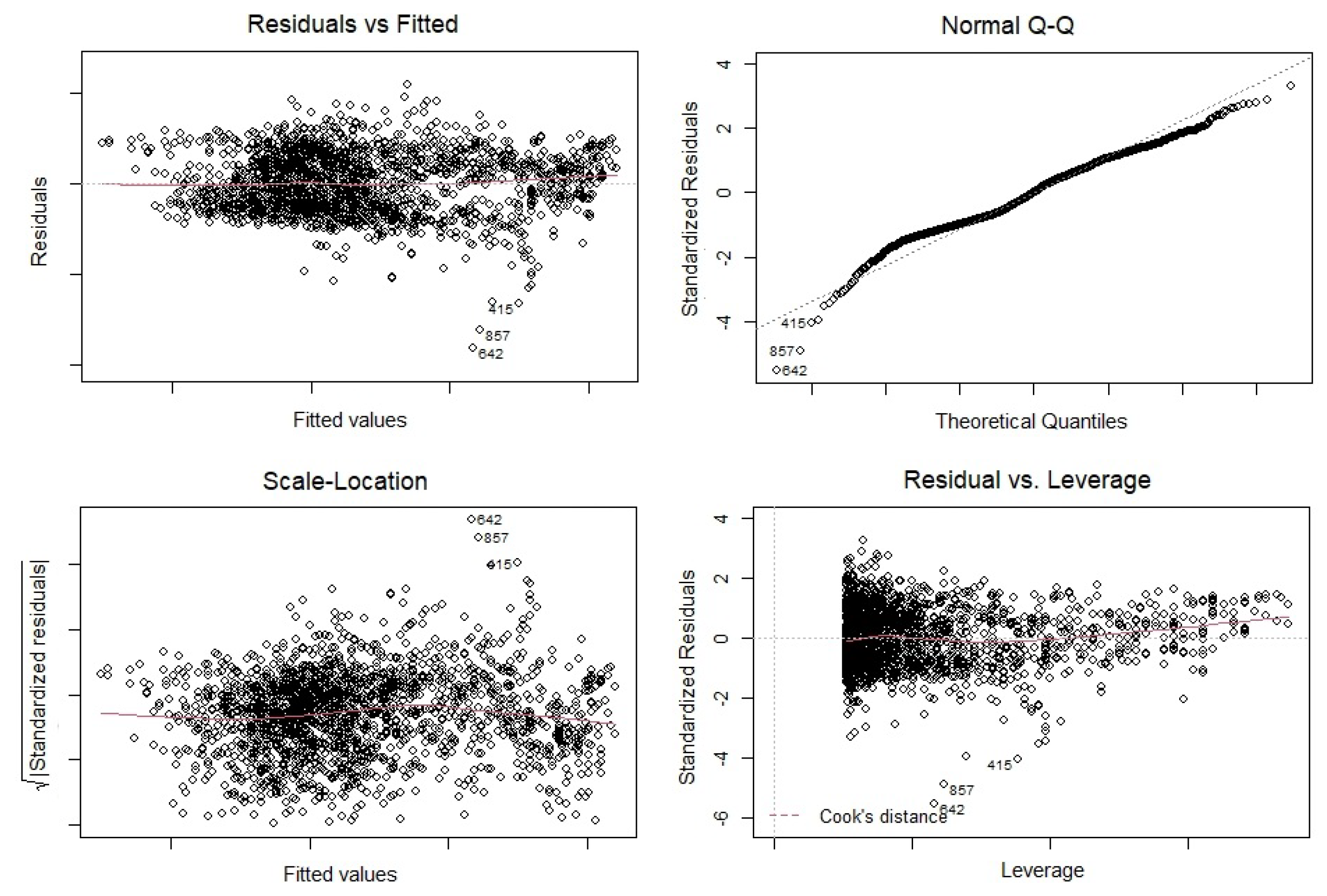
Figure A3.
The diagnostic plots of the time series linear regression model for Land Surface Temperature (LST) data for April from Figure 3.
Figure A3.
The diagnostic plots of the time series linear regression model for Land Surface Temperature (LST) data for April from Figure 3.
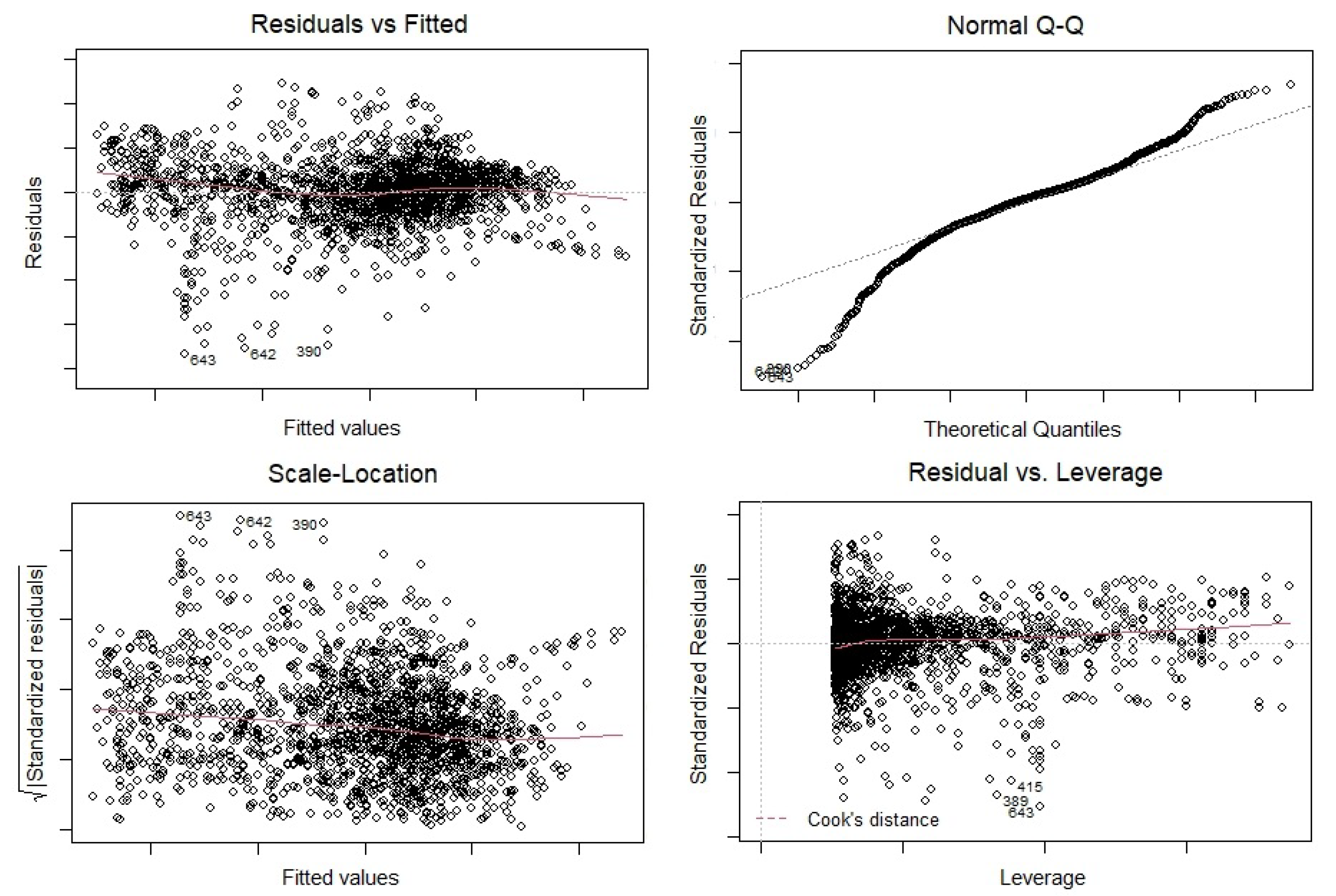
Figure A4.
The diagnostic plots of the time series linear regression model for Land Surface Temperature (LST) data for July from Figure 3.
Figure A4.
The diagnostic plots of the time series linear regression model for Land Surface Temperature (LST) data for July from Figure 3.
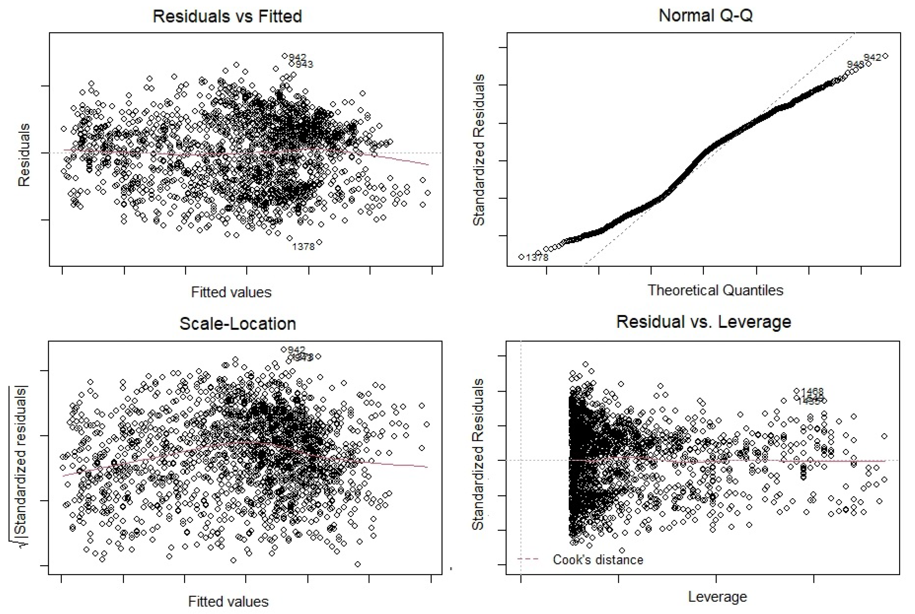
Figure A5.
The diagnostic plots of the time series linear regression model for Land Surface Temperature (LST) data for October from Figure 3.
Figure A5.
The diagnostic plots of the time series linear regression model for Land Surface Temperature (LST) data for October from Figure 3.

Figure A6.
Histogram of LST values during February, April, July, and October (2021) from Figure 3.
Figure A6.
Histogram of LST values during February, April, July, and October (2021) from Figure 3.
References
- Houghton, J.T.; Jenkins, G.J.; Ephraums, J.J. Climate change: The ipcc scientific assessment. Am. Sci. 1990. Available online: https://www.osti.gov/biblio/6819363 (accessed on 14 April 2023).
- Azizi, S.; Azizi, T. The fractal nature of drought: Power laws and fractal complexity of arizona drought. Eur. J. Math. Anal. 2022, 2, 17. [Google Scholar] [CrossRef]
- Eleftheriou, D.; Kiachidis, K.; Kalmintzis, G.; Kalea, A.; Bantasis, C.; Koumadoraki, P.; Spathara, M.E.; Tsolaki, A.; Tzampazidou, M.I.; Gemitzi, A. Determination of annual and seasonal daytime and nighttime trends of modis lst over greece-climate change implications. Sci. Total Environ. 2018, 616, 937–947. [Google Scholar] [CrossRef] [PubMed]
- Pachauri, R.K.; Allen, M.R.; Barros, V.R.; Broome, J.; Cramer, W.; Christ, R.; Church, J.A.; Clarke, L.; Dahe, Q.; Dasgupta, P.; et al. Climate Change 2014: Synthesis Report. Contribution of Working Groups I, II and III to the Fifth Assessment Report of the Intergovernmental Panel on Climate Change; IPCC: Geneva, Switzerland, 2014. [Google Scholar]
- Tayyebi, A.; Jenerette, G.D. Increases in the climate change adaption effectiveness and availability of vegetation across a coastal to desert climate gradient in metropolitan los angeles, ca, usa. Sci. Total Environ. 2016, 548, 60–71. [Google Scholar] [CrossRef]
- Sy, S.; de Noblet-Ducoudré, N.; Quesada, B.; Sy, I.; Dieye, A.M.; Gaye, A.T.; Sultan, B. Land-surface characteristics and climate in west africa: Models’ biases and impacts of historical anthropogenically-induced deforestation. Sustainability 2017, 9, 1917. [Google Scholar] [CrossRef] [Green Version]
- Zhang, W.; Luo, G.; Chen, C.; Ochege, F.U.; Hellwich, O.; Zheng, H.; Hamdi, R.; Wu, S. Quantifying the contribution of climate change and human activities to biophysical parameters in an arid region. Ecol. Indic. 2021, 129, 107996. [Google Scholar] [CrossRef]
- Boisier, J.; de Noblet-Ducoudré, N.; Ciais, P. Inferring past land use-induced changes in surface albedo from satellite observations: A useful tool to evaluate model simulations. Biogeosciences 2013, 10, 1501–1516. [Google Scholar] [CrossRef] [Green Version]
- Boisier, J.; de Noblet-Ducoudré, N.; Pitman, A.; Cruz, F.; Delire, C.; den Hurk, B.V.; der Molen, M.V.; Müller, C.; Voldoire, A. Attributing the impacts of land-cover changes in temperate regions on surface temperature and heat fluxes to specific causes: Results from the first lucid set of simulations. J. Geophys. Res. Atmos. 2012, 117, D12116. [Google Scholar] [CrossRef]
- de Noblet-Ducoudré, N.; Boisier, J.-P.; Pitman, A.; Bonan, G.; Brovkin, V.; Cruz, F.; Delire, C.; Gayler, V.; den Hurk, B.V.; Lawrence, P.; et al. Determining robust impacts of land-use-induced land cover changes on surface climate over north america and eurasia: Results from the first set of lucid experiments. J. Clim. 2012, 25, 3261–3281. [Google Scholar] [CrossRef] [Green Version]
- Kumar, D.; Shekhar, S. Statistical analysis of land surface temperature–vegetation indexes relationship through thermal remote sensing. Ecotoxicol. Environ. Saf. 2015, 121, 39–44. [Google Scholar] [CrossRef]
- Mostovoy, G.V.; King, R.L.; Reddy, K.R.; Kakani, V.G.; Filippova, M.G. Statistical estimation of daily maximum and minimum air temperatures from modis lst data over the state of mississippi. GISci. Remote Sens. 2006, 43, 78–110. [Google Scholar] [CrossRef] [Green Version]
- Taheri, M.; Mohammadian, A.; Ganji, F.; Bigdeli, M.; Nasseri, M. Energy-based approaches in estimating actual evapotranspiration focusing on land surface temperature: A review of methods, concepts, and challenges. Energies 2022, 15, 1264. [Google Scholar] [CrossRef]
- Chen, J.; Chen, B.; Black, T.A.; Innes, J.L.; Wang, G.; Kiely, G.; Hirano, T.; Wohlfahrt, G. Comparison of terrestrial evapotranspiration estimates using the mass transfer and penman-monteith equations in land surface models. J. Geophys. Res. Biogeosci. 2013, 118, 1715–1731. [Google Scholar] [CrossRef]
- Zhao, W.; Li, A. A review on land surface processes modelling over complex terrain. Adv. Meteorol. 2015, 2015, 607181. [Google Scholar] [CrossRef] [Green Version]
- Mandelbrot, B.B.; Mandelbrot, B.B. The Fractal Geometry of Nature; WH Freeman: New York, NY, USA, 1982; Volume 1. [Google Scholar]
- Mandelbrot, B.B. Fractal Geometry and Applications: A Jubilee of Benoît Mandelbrot; American Mathematical Soc.: Providence, RI, USA, 2004. [Google Scholar]
- Ivanov, P.C.; Amaral, L.A.N.; Goldberger, A.L.; Havlin, S.; Rosenblum, M.G.; Struzik, Z.R.; Stanley, H.E. Multifractality in human heartbeat dynamics. Nature 1999, 399, 461–465. [Google Scholar] [CrossRef] [PubMed] [Green Version]
- Lin, D.; Sharif, A. Common multifractality in the heart rate variability and brain activity of healthy humans. Chaos Interdiscip. J. Nonlinear Sci. 2010, 20, 023121. [Google Scholar] [CrossRef]
- Sassi, R.; Signorini, M.G.; Cerutti, S. Multifractality and Heart Rate Variability. Chaos Interdiscip. J. Nonlinear Sci. 2009, 19, 028507. [Google Scholar] [CrossRef] [PubMed]
- Burrough, P.A. Fractal dimensions of landscapes and other environmental data. Nature 1981, 294, 240–242. [Google Scholar] [CrossRef]
- Azizi, T. Mathematical modeling of stress using fractal geometry; the power laws and fractal complexity of stress. Adv. Neurol. Sci. 2022, 5, 140–148. [Google Scholar]
- Azizi, T. Measuring fractal dynamics of fecg signals to determine the complexity of fetal heart rate. Chaos Solitons Fractals X 2022, 9, 100083. [Google Scholar] [CrossRef]
- Azizi, T. On the fractal geometry of different heart rhythms. Chaos Solitons Fractals X 2022, 9, 100085. [Google Scholar] [CrossRef]
- Laguna, P.; Moody, G.B.; Mark, R.G. Power spectral density of unevenly sampled data by least-square analysis: Performance and application to heart rate signals. IEEE Trans. Biomed. Eng. 1998, 45, 698–715. [Google Scholar] [CrossRef] [PubMed]
- Martin, R. Noise power spectral density estimation based on optimal smoothing and minimum statistics. IEEE Trans. Speech Audio Process. 2001, 9, 504–512. [Google Scholar] [CrossRef] [Green Version]
- Gorelick, N.; Hancher, M.; Dixon, M.; Ilyushchenko, S.; Thau, D.; Moore, R. Google earth engine: Planetary-scale geospatial analysis for everyone. Remote Sens. Environ. 2017, 202, 18–27. [Google Scholar] [CrossRef]
- Greene, W.H. The econometric approach to efficiency analysis. Meas. Product. Effic. Product. Growth 2008, 1, 92–250. [Google Scholar]
- Cohen, L. Time-Frequency Analysis; Prentice Hall: Hoboken, NJ, USA, 1995; Volume 778. [Google Scholar]
- Gröchenig, K. Foundations of Time-Frequency Analysis; Springer Science & Business Media: Berlin/Heidelberg, Germany, 2001. [Google Scholar]
- Cooper, G.; Cowan, D. Comparing time series using wavelet-based semblance analysis. Comput. Geosci. 2008, 34, 95–102. [Google Scholar] [CrossRef]
- Mallat, S. A Wavelet Tour of Signal Processing; Elsevier: Amsterdam, The Netherlands, 1999. [Google Scholar]
- Blackledge, J. Electromagnetic Scattering Solutions for Digital Signal Processing. Ph.D. Thesis, University of JyväSkylä, JyväSkylä, Finland, 2010. [Google Scholar]
- Torrence, C.; Compo, G.P. A practical guide to wavelet analysis. Bull. Am. Meteorol. Soc. 1998, 79, 61–78. [Google Scholar] [CrossRef]
- Christensen, A.N. Semblance filtering of airborne potential field data. Aseg Ext. Abstr. 2003, 2003, 1–5. [Google Scholar] [CrossRef]
- von Frese, R.R.; Jones, M.B.; Kim, J.W.; Kim, J.-H. Analysis of anomaly correlations. Geophysics 1997, 62, 342–351. [Google Scholar] [CrossRef]
- Banerjee, S.; Hassan, M.K.; Mukherjee, S.; Gowrisankar, A. Fractal Patterns in Nonlinear Dynamics and Applications; CRC Press: Boca Raton, FL, USA, 2020. [Google Scholar]
- Arneodo, A.; Manneville, S.; Muzy, J.; Roux, S. Revealing a lognormal cascading process in turbulent velocity statistics with wavelet analysis. Philos. Trans. R. Soc. Lond. Ser. A Math. Phys. Eng. Sci. 1999, 357, 2415–2438. [Google Scholar] [CrossRef]
- Bacry, E.; Muzy, J.-F.; Arneodo, A. Singularity spectrum of fractal signals from wavelet analysis: Exact results. J. Stat. Phys. 1993, 70, 635–674. [Google Scholar] [CrossRef] [Green Version]
- Muzy, J.-F.; Bacry, E.; Arneodo, A. The multifractal formalism revisited with wavelets. Int. J. Bifurc. Chaos 1994, 4, 245–302. [Google Scholar] [CrossRef]
- Abry, P.; Baraniuk, R.; Flandrin, P.; Riedi, R.; Veitch, D. Multiscale nature of network traffic. IEEE Signal Process. Mag. 2002, 19, 28–46. [Google Scholar] [CrossRef] [Green Version]
- Abry, P.; Flandrin, P.; Taqqu, M.S.; Veitch, D. Wavelets for the analysis, estimation, and synthesis of scaling data. In Self-Similar Network Traffic and Performance Evaluation; Wiley: Hoboken, NJ, USA, 2000; pp. 39–88. [Google Scholar]
- Abry, P.; Flandrin, P.; Taqqu, M.S.; Veitch, D. Self-similarity and long-range dependence through the wavelet lens. Theory Appl.-Long-Range Depend. 2003, 1, 527–556. [Google Scholar]
- Veitch, D.; Abry, P. A wavelet-based joint estimator of the parameters of long-range dependence. IEEE Trans. Inf. Theory 1999, 45, 878–897. [Google Scholar] [CrossRef] [Green Version]
- Jaffard, S. Wavelet Techniques in Multifractal Analysis; Technical Report; Paris University: Paris, France, 2004. [Google Scholar]
- Wendt, H.; Abry, P. Multifractality tests using bootstrapped wavelet leaders. IEEE Trans. Signal Process. 2007, 55, 4811–4820. [Google Scholar] [CrossRef] [Green Version]
- Wendt, H.; Abry, P.; Jaffard, S. Bootstrap for empirical multifractal analysis. IEEE Signal Process. Mag. 2007, 24, 38–48. [Google Scholar] [CrossRef]
- Halsey, T.C.; Jensen, M.H.; Kadanoff, L.P.; Procaccia, I.; Shraiman, B.I. Fractal measures and their singularities: The characterization of strange sets. Phys. Rev. A 1986, 3, 1141. [Google Scholar] [CrossRef]
- Hentschel, H.G.E.; Procaccia, I. The infinite number of generalized dimensions of fractals and strange attractors. Phys. D Nonlinear Phenom. 1983, 8, 435–444. [Google Scholar] [CrossRef]
- Riedi, R. An improved multifractal formalism and self-similar measures. J. Math. Anal. Appl. 1995, 189, 462–490. [Google Scholar] [CrossRef] [Green Version]
- Riedi, R.H. Multifractal Processes; Technical Report; Rice Univ Houston Tx Dept of Electrical and Computer Engineering: Houston, TX, USA, 1999. [Google Scholar]
- Panigrahy, C.; Garcia-Pedrero, A.; Seal, A.; Rodríguez-Esparragón, D.; Mahato, N.K.; Gonzalo-Martín, C. An approximated box height for differential-box-counting method to estimate fractal dimensions of gray-scale images. Entropy 2017, 19, 534. [Google Scholar] [CrossRef] [Green Version]
- Gao, J.; Cao, Y.; Tung, W.-W.; Hu, J. Multiscale Analysis of Complex Time Series: Integration of Chaos and Random fractal Theory, and Beyond; John Wiley & Sons: Hoboken, NJ, USA, 2007. [Google Scholar]
- Öztürk, Y. Fractal dimension as a diagnostic tool for cardiac diseases. Int. J. Curr. Eng. Technol. 2019, 9, 425–431. [Google Scholar] [CrossRef]
- Higuchi, T. Approach to an irregular time series on the basis of the fractal theory. Phys. D Nonlinear Phenom. 1988, 31, 277–283. [Google Scholar] [CrossRef]
- Katz, M.J. Fractals and the analysis of waveforms. Comput. Biol. Med. 1988, 18, 145–156. [Google Scholar] [CrossRef] [PubMed]
- Li, Z.-L.; Tang, B.-H.; Wu, H.; Ren, H.; Yan, G.; Wan, Z.; Trigo, I.F.; Sobrino, J.A. Satellite-derived land surface temperature: Current status and perspectives. Remote Sens. Environ. 2013, 131, 14–37. [Google Scholar] [CrossRef] [Green Version]
Figure 1.
Seasonal trends in the Land Surface Temperature (LST) in Riley County in the US state of Kansas obtained via the Google Earth Engine for winter 2021–winter 2022.
Figure 1.
Seasonal trends in the Land Surface Temperature (LST) in Riley County in the US state of Kansas obtained via the Google Earth Engine for winter 2021–winter 2022.

Figure 2.
Study area in the Riley County and Land Surface Temperature (LST) maps (a) The LST map for February 2021; (b) the LST map for April 2021; (c) the LST map for July 2021; (d) the LST map for October 2021.
Figure 2.
Study area in the Riley County and Land Surface Temperature (LST) maps (a) The LST map for February 2021; (b) the LST map for April 2021; (c) the LST map for July 2021; (d) the LST map for October 2021.
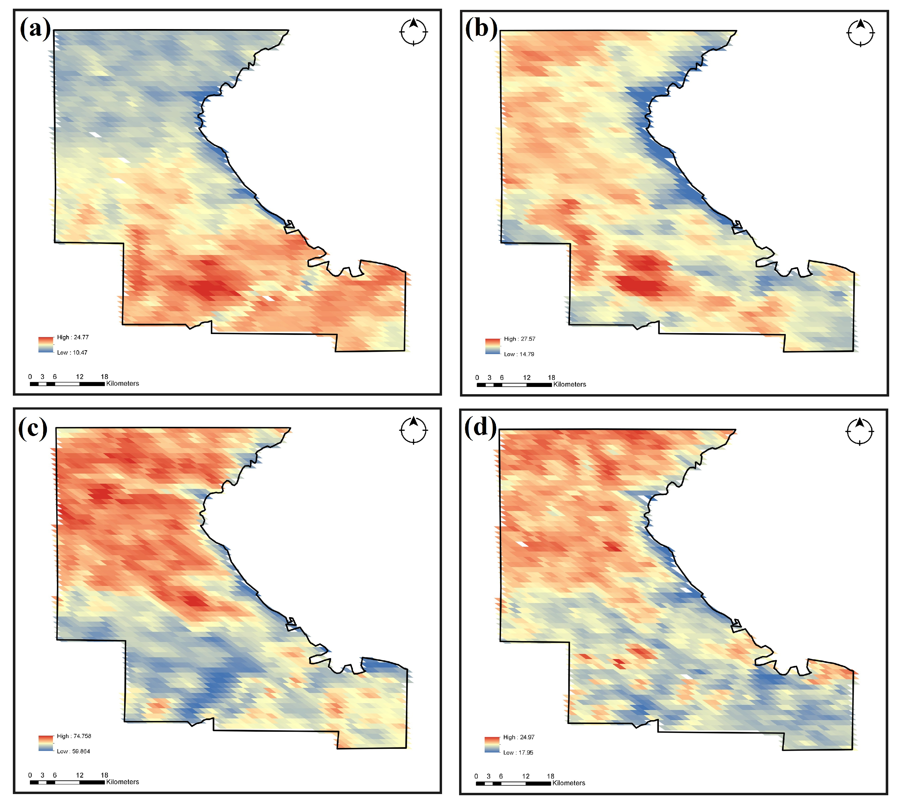
Figure 3.
Scatter plot of the Land Surface Temperature (LST) in Riley County during February, April, July, and October (2021) obtained via Google Earth Engine.
Figure 3.
Scatter plot of the Land Surface Temperature (LST) in Riley County during February, April, July, and October (2021) obtained via Google Earth Engine.
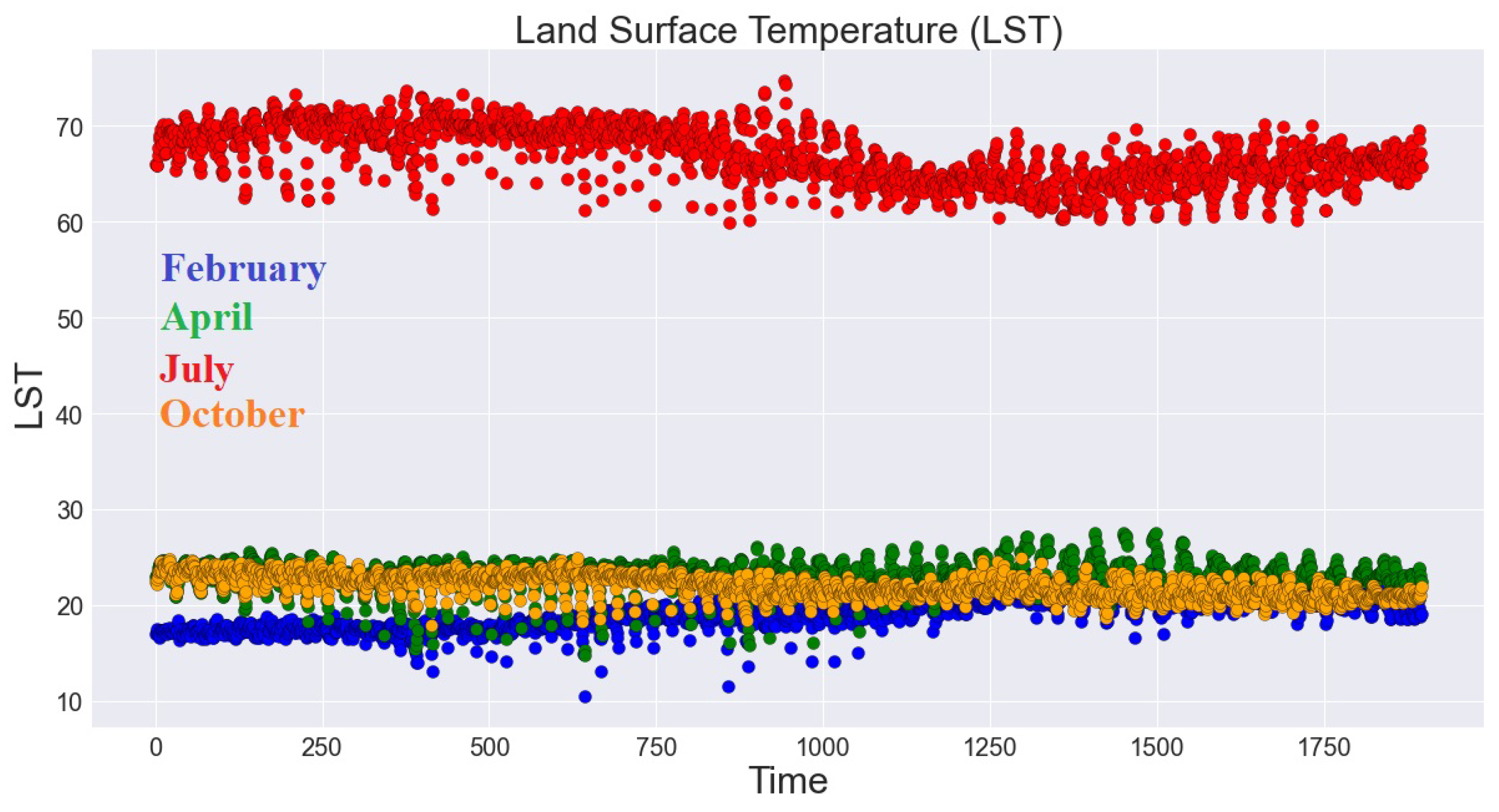
Figure 4.
The Schematic diagram of the Land Surface Temperature (LST) nonlinear analysis (accessed on 21 October 2021 https://earthobservatory.nasa.gov/global-maps/MOD_LSTD_M).
Figure 4.
The Schematic diagram of the Land Surface Temperature (LST) nonlinear analysis (accessed on 21 October 2021 https://earthobservatory.nasa.gov/global-maps/MOD_LSTD_M).
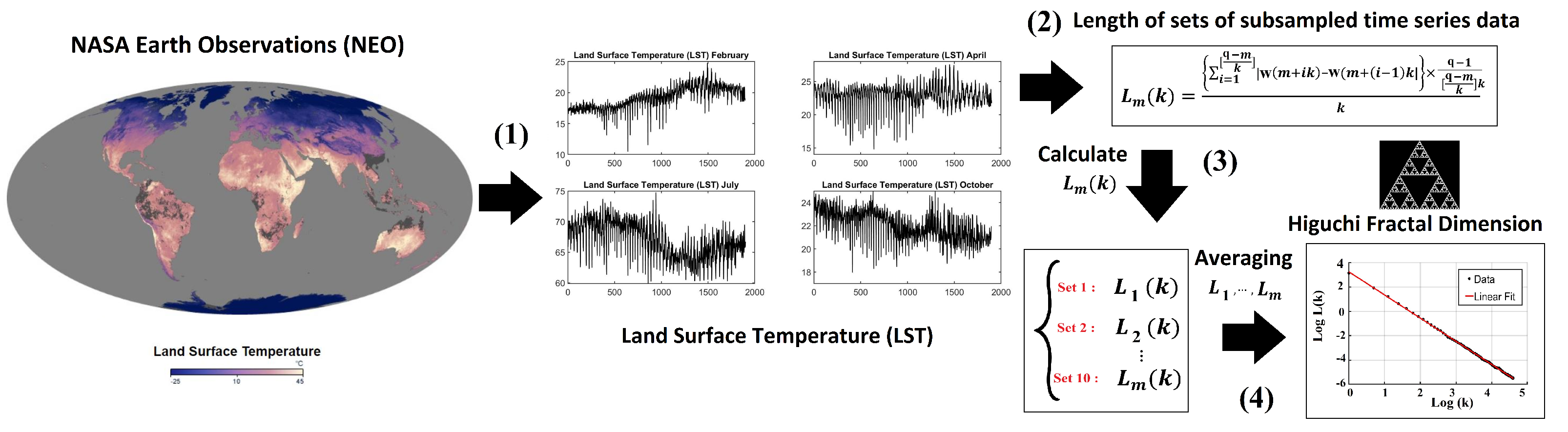
Figure 5.
Time series nonlinear regression model (2) using the Land Surface Temperature (LST) in Riley County during February, April, July, and October (2021) obtained via Google Earth Engine.
Figure 5.
Time series nonlinear regression model (2) using the Land Surface Temperature (LST) in Riley County during February, April, July, and October (2021) obtained via Google Earth Engine.

Figure 6.
Time–frequency representations of the Land Surface Temperature (LST) in Riley County during February, April, July, and October (2021) using the Continuous Wavelet Transform (CWT) in three-dimensional Time–Frequency–Magnitude space.
Figure 6.
Time–frequency representations of the Land Surface Temperature (LST) in Riley County during February, April, July, and October (2021) using the Continuous Wavelet Transform (CWT) in three-dimensional Time–Frequency–Magnitude space.
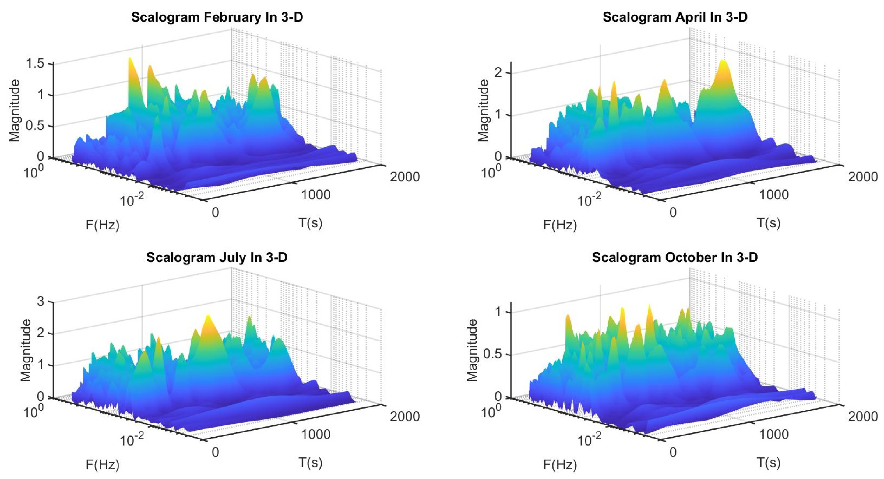
Figure 7.
Semblance of the LST datasets shown in Figure 3 to find the correlation between LST data and height of each grid point in LST grid cells, computed using the vector dot product of the two complex wavelet vectors (9). The correlation varies as a function of time and wavelength. Strong correlations on larger wavelengths () are presented in dark red, positive correlations () are presented in yellow, and zero correlations () are presented in green. The results show mostly dark red, implying strong positive correlations between LST data and the height of each grid point in LST grid cells.

Figure 8.
Power Law or self–similarity patterns; fitted least–squares approximation for the logarithm of the power spectral density of the Land Surface Temperature (LST) in Riley County during February, April, July, and October (2021) obtained by wavelet techniques.
Figure 8.
Power Law or self–similarity patterns; fitted least–squares approximation for the logarithm of the power spectral density of the Land Surface Temperature (LST) in Riley County during February, April, July, and October (2021) obtained by wavelet techniques.

Figure 9.
Scaling exponent of the power spectral density of the Land Surface Temperature (LST) in Riley County during February, April, July, and October (2021).
Figure 9.
Scaling exponent of the power spectral density of the Land Surface Temperature (LST) in Riley County during February, April, July, and October (2021).
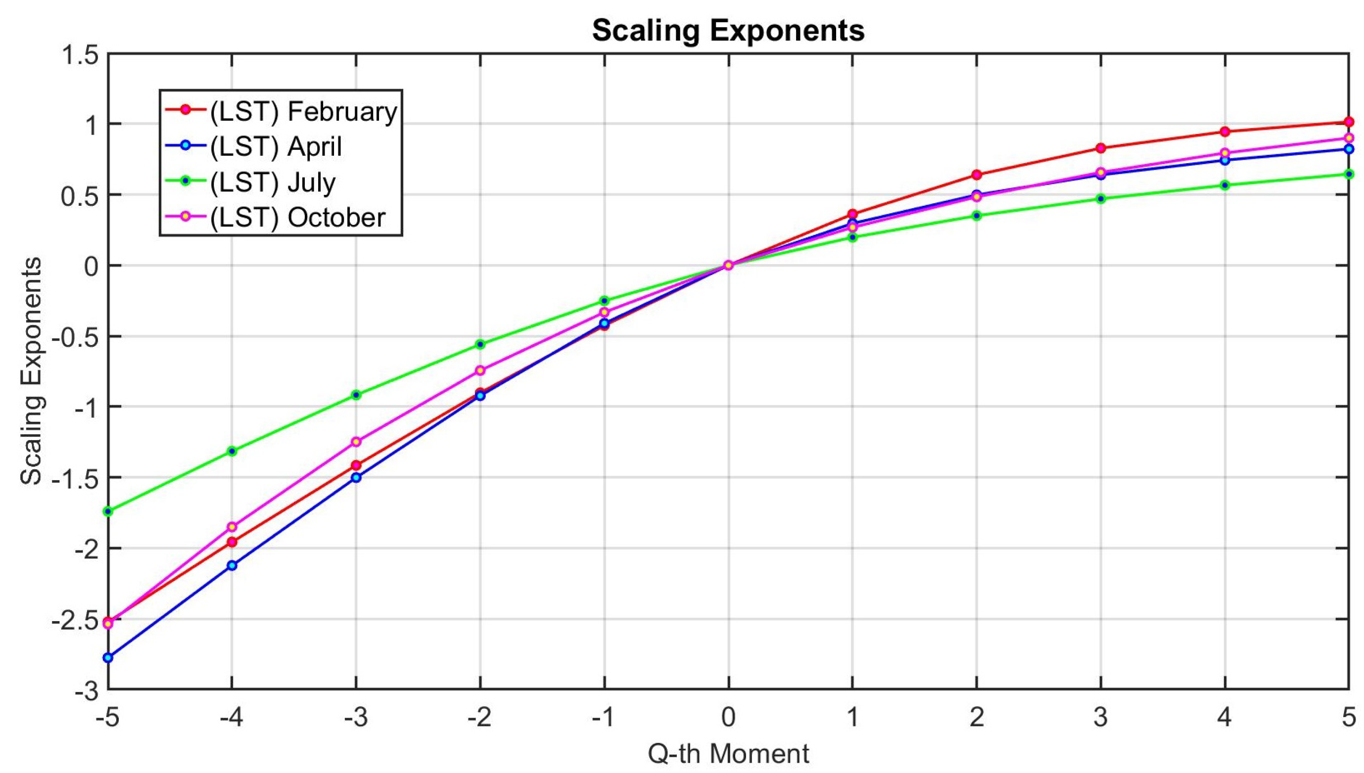
Figure 10.
The multi–fractal spectrum analysis of the Land Surface Temperature (LST) in Riley County during February, April, July, and October (2021) shows the occurrence of a mono–fractal process with a narrow range of exponents for all four groups of LST time series data.
Figure 10.
The multi–fractal spectrum analysis of the Land Surface Temperature (LST) in Riley County during February, April, July, and October (2021) shows the occurrence of a mono–fractal process with a narrow range of exponents for all four groups of LST time series data.
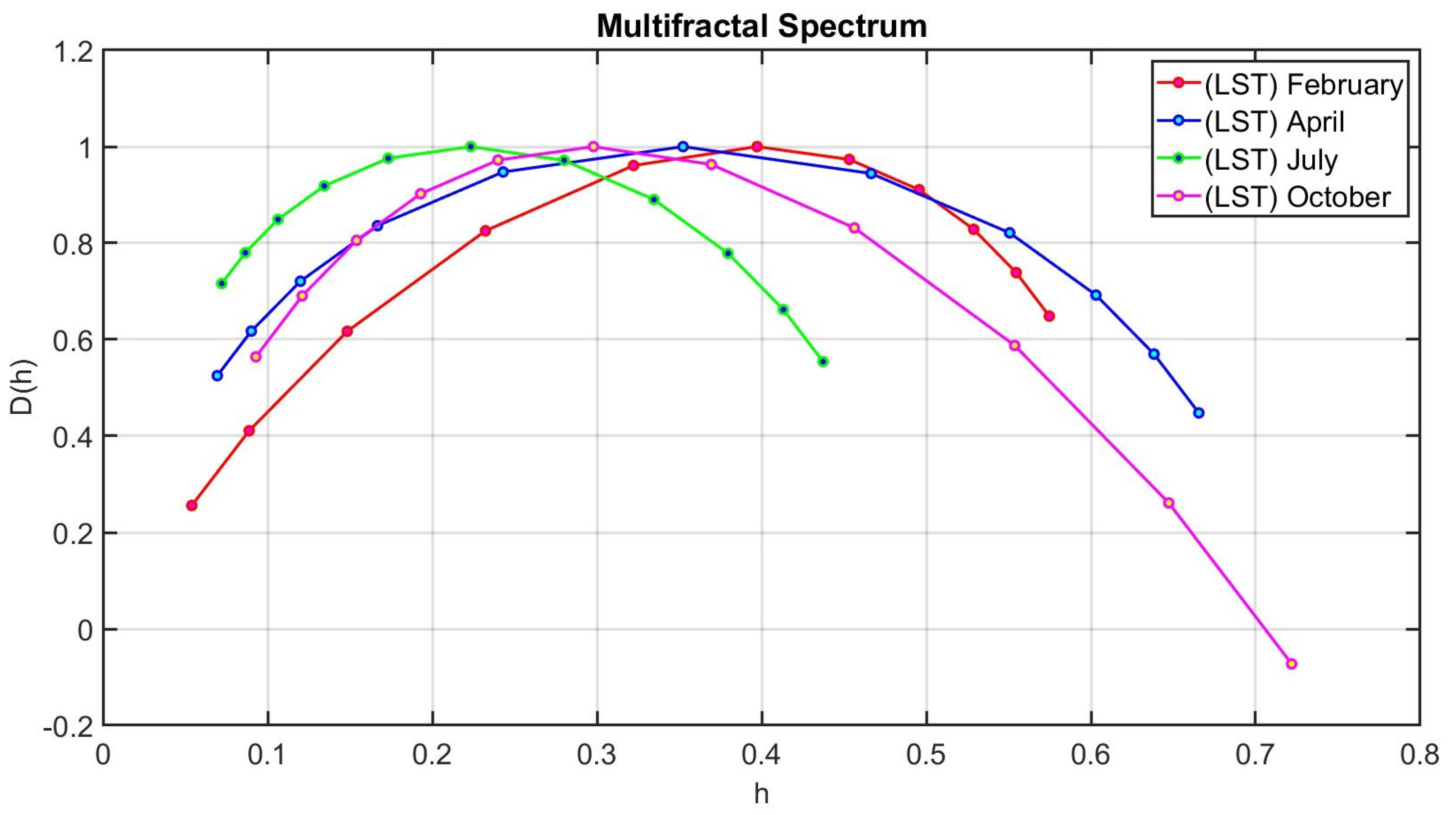
Figure 11.
Plots of versus for time interval , the logarithmic scale and the corresponding slope of fitted regression line (the Higuchi fractal dimension) of the Land Surface Temperature (LST) of Riley County during February, April, July and October (2021).
Figure 11.
Plots of versus for time interval , the logarithmic scale and the corresponding slope of fitted regression line (the Higuchi fractal dimension) of the Land Surface Temperature (LST) of Riley County during February, April, July and October (2021).
Disclaimer/Publisher’s Note: The statements, opinions and data contained in all publications are solely those of the individual author(s) and contributor(s) and not of MDPI and/or the editor(s). MDPI and/or the editor(s) disclaim responsibility for any injury to people or property resulting from any ideas, methods, instructions or products referred to in the content. |
© 2023 by the authors. Licensee MDPI, Basel, Switzerland. This article is an open access article distributed under the terms and conditions of the Creative Commons Attribution (CC BY) license (https://creativecommons.org/licenses/by/4.0/).
Share and Cite
MDPI and ACS Style
Azizi, S.; Azizi, T. Noninteger Dimension of Seasonal Land Surface Temperature (LST). Axioms 2023, 12, 607. https://doi.org/10.3390/axioms12060607
AMA Style
Azizi S, Azizi T. Noninteger Dimension of Seasonal Land Surface Temperature (LST). Axioms. 2023; 12(6):607. https://doi.org/10.3390/axioms12060607
Chicago/Turabian StyleAzizi, Sepideh, and Tahmineh Azizi. 2023. "Noninteger Dimension of Seasonal Land Surface Temperature (LST)" Axioms 12, no. 6: 607. https://doi.org/10.3390/axioms12060607
Note that from the first issue of 2016, this journal uses article numbers instead of page numbers. See further details here.