Solutions of (2+1)-D & (3+1)-D Burgers Equations by New Laplace Variational Iteration Technique

Abstract

The new Laplace variational iterative method is used in this research for solving the (2+1)-D and (3+1)-D Burgers equations. This technique relies on the modified variational iteration method and the Laplace transform. To apply this approach, the differential problem is first transformed into an algebraic form using the Laplace transform, and then the algebraic equations are iteratively solved using the modified variational iterative approach. By utilizing this technique, the Burgers equations can be solved both numerically and analytically. The study demonstrates the effectiveness of the new Laplace variational iterative approach through three specific examples.

1. Introduction

The J.M. Burgers equation, also known as Burgers’s equation, is a significant and commonly used non-linear PDE. It was first introduced by Bateman and later corrected by Burgers, and is sometimes referred to as the Bateman–Burgers equation. This equation is employed to simulate numerous physical phenomena, for example, acoustics, diffraction water waves, heat conduction, shock waves, and turbulence issues, among others.

This research focuses on the analytical solutions of the two-dimensional and three-dimensional Burgers equations. The new Laplace transform with the variational iteration method (LVIM) is utilized for solving these equations. Approximate results obtained using the LVIM approach are then compared with the analytical results of Burgers’s equation, the numerical approximations of the Burgers equation obtained via the Laplace Homotopy Perturbation method (LHPM) [1], and the numerical results of the Burgers equation obtained via the EHPM [2]. To demonstrate the effectiveness of the proposed method, a comparison study is given in Section 3.

In addition, the suggested strategy’s convergence is illustrated through graphs of both precise and approximate solutions. Various partial differential equations with linear and non-linear coefficients can be utilized to solve initial value and boundary value problems. To find approximate solutions to Burgers equations, several numerical schemes have been developed, including the spline FEM, ADM, Douglas FD scheme, exact explicit FDM, VIM, and others [3,4,5,6,7,8,9,10]. However, only a few analytical methods, such as the LHPM [11], Hopf–Cole Transformation [12], etc., have been developed to obtain the precise solution of certain PDEs. Laplace transform-based methods are extensively employed in mathematics to solve differential equations. Other techniques, such as the VIM and the HPM, can also be combined with it to make it hybrid. By combining these approaches with the Laplace Transform method, partial differential equations can be solved analytically. The VIM has been used to solve various differential equations [13]. It has been demonstrated that the VIM can also solve non-linear equations [14]. The Laplace Transformation and variational iteration approach have been used to solve Smoluchowski’s coagulation equations [15]. A new modified variational iterative approach has been proposed for the solution of boundary value problems of higher order [16]. The variational iteration approach and Laplace transformation have been combined in [17]. In [18], certain issues with the variational iterative approach and how the Laplace transform method fixes them are detailed. Modified fractional derivatives have a Laplace variational approach built into them [19]. A new Laplace Transformation and variational iterative approach can solve non-linear PDEs [20]. The new Laplace and variational iterative approach has been used to solve numerous equations [21,22,23,24].

Consider, the (2+1)-D non-linear Burgers’s equation can also be written as

$$\frac{\partial \phi \left(\alpha ,\beta ,\tau \right)}{\partial \tau }+\rho \phi \left(\alpha ,\beta ,\tau \right)\frac{\partial \phi \left(\alpha ,\beta ,\tau \right)}{\partial \alpha }=\mu \left(\frac{{\partial }^2\phi \left(\alpha ,\beta ,\tau \right)}{\partial {\alpha }^2}+\frac{{\partial }^2\phi \left(\alpha ,\beta ,\tau \right)}{\partial {\beta }^2}\right)$$

(1)

with the initial conditions

$$\phi \left(\alpha ,\beta ,0\right)=h\left(\alpha ,\beta \right)$$

where $u$ is the velocity component, $\mu$ is the kinematic viscosity, $\rho$ is any constant, and $t$ is the time.

Similarly, the (3+1)-D Non-linear Burgers equation is

$$\frac{\partial \phi \left(\alpha ,\beta ,z,\tau \right)}{\partial \tau }+\rho \phi \left(\alpha ,\beta ,z,\tau \right)\frac{\partial \phi \left(\alpha ,\beta ,z,\tau \right)}{\partial \alpha }=\mu \left(\frac{{\partial }^2\phi \left(\alpha ,\beta ,z,\tau \right)}{\partial {\alpha }^2}+\frac{{\partial }^2\phi \left(\alpha ,\beta ,z,\tau \right)}{\partial {\beta }^2}+\frac{{\partial }^2\phi \left(\alpha ,\beta ,z,\tau \right)}{\partial z^2}\right)$$

with initial conditions

$$\phi \left(\alpha ,\beta ,z,0\right)=j\left(\alpha ,\beta ,z\right)$$

where $u$ is the velocity component, $\mu$ is the kinematic viscosity, $\rho$ is any constant, and $\tau$ is the time.

Non-linear partial differential equations find wide application in the fields of engineering, physics, and applied mathematics. Various approaches have been suggested in the literature to solve the two-dimensional Burgers equations as well as the two-dimensional and three-dimensional Burgers equations. The importance of discovering exact solutions to PDEs for developing novel techniques to obtain precise or approximate solutions remains a topic of great interest in mathematics, engineering, and physics, as evidenced by recent publications [25,26,27,28,29,30].

2. Materials and Methods

2.1. New LVIM for Solving (2+1)-D Burgers’s Equation

Consider the following (2+1)-D Burgers equation:

$$\frac{\partial \phi \left(\alpha ,\beta ,\tau \right)}{\partial \tau }+\rho \phi \left(\alpha ,\beta ,\tau \right)\frac{\partial \phi \left(\alpha ,\beta ,\tau \right)}{\partial \alpha }=\mu \left(\frac{{\partial }^2\phi \left(\alpha ,\beta ,\tau \right)}{\partial {\alpha }^2}+\frac{{\partial }^2\phi \left(\alpha ,\beta ,\tau \right)}{\partial {\beta }^2}\right)$$

(2)

with given conditions as

$$\phi \left(\alpha ,\beta ,0\right)=h\left(\alpha ,\beta \right)$$

Rewriting Equation (2), we have

$$\frac{\partial \phi \left(\alpha ,\beta ,\tau \right)}{\partial \tau }=\mu \left(\frac{{\partial }^2\phi \left(\alpha ,\beta ,\tau \right)}{\partial {\alpha }^2}+\frac{{\partial }^2\phi \left(\alpha ,\beta ,\tau \right)}{\partial {\beta }^2}\right)-\rho \phi \left(\alpha ,\beta ,\tau \right)\frac{\partial \phi \left(\alpha ,\beta ,\tau \right)}{\partial \alpha }$$

(3)

By applying Laplace transformation on (3), we have

$$L\left\{\frac{\partial \phi \left(\alpha ,\beta ,\tau \right)}{\partial \tau }\right\}=L\left\{\mu \left(\frac{{\partial }^2\phi \left(\alpha ,\beta ,\tau \right)}{\partial {\alpha }^2}+\frac{{\partial }^2\phi \left(\alpha ,\beta ,\tau \right)}{\partial {\beta }^2}\right)-\rho \phi \left(\alpha ,\beta ,\tau \right)\frac{\partial \phi \left(\alpha ,\beta ,\tau \right)}{\partial \alpha }\right\}$$

(4)

$$sL\left\{\phi \left(\alpha ,\beta ,\tau \right)\right\}-\phi \left(\alpha ,\beta ,0\right)=L\left\{\mu \left(\frac{{\partial }^2\phi }{\partial {\alpha }^2}+\frac{{\partial }^2\phi }{\partial {\beta }^2}\right)-\rho \phi \frac{\partial \phi }{\partial \alpha }\right\}$$

(5)

$$sL\left\{\phi \left(\alpha ,\beta ,\tau \right)\right\}-h\left(\alpha ,\beta \right)=L\left\{\mu \left(\frac{{\partial }^2\phi }{\partial {\alpha }^2}+\frac{{\partial }^2\phi }{\partial {\beta }^2}\right)-\rho \phi \frac{\partial \phi }{\partial \alpha }\right\}$$

(6)

$$sL\left\{\phi \left(\alpha ,\beta ,\tau \right)\right\}=h\left(\alpha ,\beta \right)+L\left\{\mu \left(\frac{{\partial }^2\phi }{\partial {\alpha }^2}+\frac{{\partial }^2\phi }{\partial {\beta }^2}\right)-\rho \phi \frac{\partial \phi }{\partial \alpha }\right\}$$

(7)

$$L\left\{\phi \left(\alpha ,\beta ,\tau \right)\right\}=\frac{h\left(\alpha ,\beta \right)}{s}+\frac{1}{s}L\left\{\mu \left(\frac{{\partial }^2\phi }{\partial {\alpha }^2}+\frac{{\partial }^2\phi }{\partial {\beta }^2}\right)-\rho \phi \frac{\partial \phi }{\partial \alpha }\right\}$$

(8)

By using inverse Laplace transformation on (8), we obtain

$$\phi \left(\alpha ,\beta ,\tau \right)=h\left(\alpha ,\beta \right)+L^{-1}\left[\frac{1}{s}L\left\{\mu \left(\frac{{\partial }^2\phi }{\partial {\alpha }^2}+\frac{{\partial }^2\phi }{\partial {\beta }^2}\right)-\rho \phi \frac{\partial \phi }{\partial \alpha }\right\}\right]$$

(9)

Now, by modifying VIM from Equation (9), we obtain

$${\phi }_{n+1}=h\left(\alpha ,\beta \right)+L^{-1}\left[\frac{1}{s} L \left\{\mu \left(\frac{{\partial }^2{\phi }_n}{\partial {\alpha }^2}+\frac{{\partial }^2{\phi }_n}{\partial {\beta }^2}\right)-\left(\rho {\phi }_n\frac{\partial {\phi }_n}{\partial \alpha }\right)\right\}\right]$$

(10)

Equation (10) represents the modified iteration formula of LVIM; the solution is given by

$$\phi =\underset{n\to \infty }{\lim }{\phi }_n$$

2.2. The Convergence of LVIM for (2+1)-D Partial Differential Equations

Consider the two-dimensional differential equation

$$\mathit{l}\phi \left(\alpha ,\beta ,\tau \right)+\mathit{n}\phi \left(\alpha ,\beta ,\tau \right)=\mathit{g}\left(\alpha ,\beta ,\tau \right)$$

(11)

with the initial conditions

$$\phi \left(\alpha ,\beta ,0\right)=\mathit{h}\left(\alpha ,\beta \right)$$

(12)

where l, n, and g are a linear operator of the first order, a non-linear operator, and a non-homogeneous term, respectively.

The iteration formula of the new LVIM is

$${\phi }_{m+1}\left(\alpha ,\beta ,\tau \right)=G\left(\alpha ,\beta \right)+L^{-1}\left[\frac{1}{s}L\left\{\mathit{n}{\phi }_m\left(\alpha ,\beta ,\tau \right)\right\}\right]$$

Now, define the operator $A\left[\phi \right]$ as

$$A\left[\phi \right]=L^{-1}\left[\frac{1}{s}L\left\{\mathit{n}{\phi }_m\left(\alpha ,\beta ,\tau \right)\right\}\right]$$

(13)

define the components $v_m,m=0,1,2,3\dots$ as

$$\left\{\begin{array}{c}{v}_0=u_0,\\ v_1=A\left[v_0\right],\\ v_2=A\left[v_1\right],\\ .\\ .\\ .\\ v_{m+1}=A\left[v_m\right]\end{array}\right.$$

(14)

Hence,

$$\phi \left(\alpha ,\beta ,\tau \right)=\underset{m\to \infty }{\lim }{\phi }_m\left(\alpha ,\beta ,\tau \right)$$

(15)

For the analysis of convergence of new LVIM, let us discuss the following theorem.

Theorem 1. 

Let A, as defined in (14), be an operator from Hilbert space H to H; the solution, as defined in (16), converges if there exists $0<\gamma <1$  such that

$$\Vert A\left[v_{m+1}\right]\Vert \le \gamma \Vert A\left[v_m\right]\Vert \left(i.e., \Vert v_{m+1}\Vert \le \gamma \Vert v_m\Vert \right)$$

  for all $m\in N\cup \left\{0\right\}$.

Proof. 

Define the sequence ${\left\{S_n\right\}}_{n=1}^{\infty }$ as

$$\left\{\begin{array}{c}{S}_1=G\left(\alpha ,\beta \right)+v_{1,}\\ S_2=G\left(\alpha ,\beta \right)+v_{2,}\\ S_3=G\left(\alpha ,\beta \right)+v_{3,}\\ .\\ .\\ .\\ S_m=G\left(\alpha ,\beta \right)+v_m\end{array}\right.$$

(16)

Now, we will show that sequence ${\left\{S_n\right\}}_{n=1}^{\infty }$ is a Cauchy sequence in the Hilbert space H.

Consider

$$\Vert S_{m+1}-S_m\Vert =\Vert v_{m+1}-v_m\Vert \le \gamma \Vert v_m\Vert \le {\gamma }^2\Vert v_{m-1}\Vert \le \dots \le {\gamma }^{m+1}\Vert v_0\Vert$$

For every $m,n\in N,m\ge n$, we have

$$\begin{array}{cc}\hfill \Vert S_m-S_n\Vert & =\Vert (S_m-S_{m-1})+(S_{m-1}-S_{m-2})+\dots +(S_{n+1}-S_n)\Vert \hfill \\ & \le \Vert (S_m-S_{m-1})\Vert +\Vert (S_{m-1}-S_{m-2})\Vert +\dots +\Vert (S_{n+1}-S_n)\Vert \hfill \\ & \le {\gamma }^m\Vert v_0\Vert +{\gamma }^{m-1}\Vert v_0\Vert +\dots +{\gamma }^{n+1}\Vert v_0\Vert \hfill \\ & =\frac{1-{\gamma }^{m-n}}{1-\gamma }{\gamma }^{n+1}\Vert v_0\Vert \hfill \end{array}$$

Since $0<\gamma <1$, therefore,

$$\underset{m,n\to \infty }{\lim }\Vert S_m-S_n\Vert =0$$

(17)

Hence, ${\left\{S_n\right\}}_{n=1}^{\infty }$ is a Cauchy sequence in the Hilbert space H and it implies that the series solution (16) converges. □

2.3. New LVIM for Solving (3+1)-D Burgers’s Equation

Consider the following (3+1)-D Burgers equation:

$$\frac{\partial \phi \left(\alpha ,\beta ,\tau ,z\right)}{\partial \tau }+\rho \phi \left(\alpha ,\beta ,z,\tau \right)\frac{\partial \phi \left(\alpha ,\beta ,z,\tau \right)}{\partial \alpha }=\mu \left(\frac{{\partial }^2\phi \left(\alpha ,\beta ,z,\tau \right)}{\partial {\alpha }^2}+\frac{{\partial }^2\phi \left(\alpha ,\beta ,z,\tau \right)}{\partial {\beta }^2}+\frac{{\partial }^2\phi \left(\alpha ,\beta ,z,\tau \right)}{\partial z^2}\right)$$

(18)

with given conditions as

$$\phi \left(\alpha ,\beta ,z,0\right)=j\left(\alpha ,\beta ,z\right)$$

Rewriting Equation (18), we have

$$\frac{\partial \phi \left(\alpha ,\beta ,z,\tau \right)}{\partial \tau }=\mu \left(\frac{{\partial }^2\phi \left(\alpha ,\beta ,z,\tau \right)}{\partial {\alpha }^2}+\frac{{\partial }^2\phi \left(\alpha ,\beta ,z,\tau \right)}{\partial {\beta }^2}+\frac{{\partial }^2\phi \left(\alpha ,\beta ,z,\tau \right)}{\partial z^2}\right)-\rho \phi \left(\alpha ,\beta ,z,\tau \right)\frac{\partial \phi \left(\alpha ,\beta ,z,\tau \right)}{\partial \alpha }$$

(19)

By applying Laplace transformation on (19), we have

$$\begin{array}{cc}\hfill L\left\{\frac{\partial \phi \left(\alpha ,\beta ,z,\tau \right)}{\partial \tau }\right\}& \\ & =L\left\{\mu \left(\frac{{\partial }^2\phi \left(\alpha ,\beta ,z,\tau \right)}{\partial {\alpha }^2}+\frac{{\partial }^2\phi \left(\alpha ,\beta ,z,\tau \right)}{\partial {\beta }^2}+\frac{{\partial }^2\phi \left(\alpha ,\beta ,z,\tau \right)}{\partial z^2}\right)-\rho \phi \left(\alpha ,\beta ,z,\tau \right)\frac{\partial \phi \left(\alpha ,\beta ,z,\tau \right)}{\partial \alpha }\right\}\hfill \end{array}$$

(20)

$$sL\left\{\phi \left(\alpha ,\beta ,z,\tau \right)\right\}-\phi \left(\alpha ,\beta ,z,0\right)=L\left\{\mu \left(\frac{{\partial }^2\phi }{\partial {\alpha }^2}+\frac{{\partial }^2\phi }{\partial {\beta }^2}+\frac{{\partial }^2\phi }{\partial z^2}\right)-\rho \phi \frac{\partial \phi }{\partial \alpha }\right\}$$

(21)

$$sL\left\{\phi \left(\alpha ,\beta ,z,\tau \right)\right\}-j\left(\alpha ,\beta ,z\right)=L\left\{\mu \left(\frac{{\partial }^2\phi }{\partial {\alpha }^2}+\frac{{\partial }^2\phi }{\partial {\beta }^2}+\frac{{\partial }^2\phi }{\partial z^2}\right)-\rho \phi \frac{\partial \phi }{\partial \alpha }\right\}$$

(22)

$$sL\left\{\phi \left(\alpha ,\beta ,z,\tau \right)\right\}=j\left(\alpha ,\beta ,z\right)+L\left\{\mu \left(\frac{{\partial }^2\phi }{\partial {\alpha }^2}+\frac{{\partial }^2\phi }{\partial {\beta }^2}+\frac{{\partial }^2\phi }{\partial z^2}\right)-\rho \phi \frac{\partial \phi }{\partial \alpha }\right\}$$

(23)

$$L\left\{\phi \left(\alpha ,\beta ,z,\tau \right)\right\}=\frac{j\left(\alpha ,\beta ,z\right)}{s}+\frac{1}{s}L\left\{\mu \left(\frac{{\partial }^2\phi }{\partial {\alpha }^2}+\frac{{\partial }^2\phi }{\partial {\beta }^2}+\frac{{\partial }^2\phi }{\partial z^2}\right)-\rho \phi \frac{\partial \phi }{\partial \alpha }\right\}$$

(24)

By using inverse Laplace transformation on (24), we obtain

$$\phi \left(\alpha ,\beta ,z,\tau \right)=j\left(\alpha ,\beta ,z\right)+L^{-1}\left[\frac{1}{s}L\left\{\mu \left(\frac{{\partial }^2\phi }{\partial {\alpha }^2}+\frac{{\partial }^2\phi }{\partial {\beta }^2}+\frac{{\partial }^2\phi }{\partial z^2}\right)-\rho \phi \frac{\partial \phi }{\partial \alpha }\right\}\right]$$

(25)

Now, by modifying VIM from Equation (25), we obtain

$${\phi }_{n+1}=j\left(\alpha ,\beta ,z\right)+L^{-1}\left[\frac{1}{s} L \left\{\mu \left(\frac{{\partial }^2{\phi }_n}{\partial {\alpha }^2}+\frac{{\partial }^2{\phi }_n}{\partial {\beta }^2}+\frac{{\partial }^2{\phi }_n}{\partial z^2}\right)-\left(\rho {\phi }_n\frac{\partial {\phi }_n}{\partial \alpha }\right)\right\}\right]$$

(26)

Equation (26) represents the modified iteration formula of LVIM; the solution is given by

$$\phi =\underset{n\to \infty }{\lim }{\phi }_n$$

(27)

2.4. The Convergence of LVIM for (3+1)-D Partial Differential Equations

Consider the three-dimensional differential equation

$$\mathit{l}\phi \left(\alpha ,\beta ,z,\tau \right)+\mathit{n}\phi \left(\alpha ,\beta ,\tau \right)=\mathit{g}\left(\alpha ,\beta ,\tau \right)$$

(28)

with the initial conditions

$$\phi \left(\alpha ,\beta ,0\right)=\mathit{h}\left(\alpha ,\beta \right)$$

(29)

where l, n, and g are a linear operator of the first order, a non-linear operator, and a non-homogeneous term, respectively.

The iteration formula of the new LVIM is

$${\phi }_{m+1}\left(\alpha ,\beta ,z,\tau \right)=G\left(\alpha ,\beta \right)+L^{-1}\left[\frac{1}{s}L\left\{\mathit{n}{\phi }_m\left(\alpha ,\beta ,z,\tau \right)\right\}\right]$$

Now, define the operator $A\left[\phi \right]$ as

$$A\left[\phi \right]=L^{-1}\left[\frac{1}{s}L\left\{\mathit{n}{\phi }_m\left(\alpha ,\beta ,z,\tau \right)\right\}\right]$$

(30)

define the components $v_m,m=0,1,2,3\dots$ as

$$\left\{\begin{array}{c}{v}_0=u_0,\\ v_1=A\left[v_0\right],\\ v_2=A\left[v_1\right],\\ .\\ .\\ .\\ v_{m+1}=A\left[v_m\right]\end{array}\right.$$

(31)

Hence,

$$\phi \left(\alpha ,\beta ,z,\tau \right)=\underset{m\to \infty }{\lim }{\phi }_m\left(\alpha ,\beta ,z,\tau \right)$$

(32)

For the analysis of convergence of new LVIM, let us discuss the following theorem.

Theorem 2. 

Let A, as defined in (30), be an operator from Hilbert space H to H; the solution, as defined in (32), converges if there exists $0<\gamma <1$ such that

$$\Vert A\left[v_{m+1}\right]\Vert \le \gamma \Vert A\left[v_m\right]\Vert \left(i.e., \Vert v_{m+1}\Vert \le \gamma \Vert v_m\Vert \right)$$

  for all $m\in N\cup \left\{0\right\}$.

Proof. 

Define the sequence ${\left\{S_n\right\}}_{n=1}^{\infty }$ as

$$\left\{\begin{array}{c}{S}_1=G\left(\alpha ,\beta ,z\right)+v_{1,}\\ S_2=G\left(\alpha ,\beta ,z\right)+v_{2,}\\ S_3=G\left(\alpha ,\beta ,z\right)+v_{3,}\\ .\\ .\\ .\\ S_m=G\left(\alpha ,\beta ,z\right)+v_m\end{array}\right.$$

(33)

Now, we will show that sequence ${\left\{S_n\right\}}_{n=1}^{\infty }$ is a Cauchy sequence in the Hilbert space H.

Consider

$$\Vert S_{m+1}-S_m\Vert =\Vert v_{m+1}-v_m\Vert \le \gamma \Vert v_m\Vert \le {\gamma }^2\Vert v_{m-1}\Vert \le \dots \le {\gamma }^{m+1}\Vert v_0\Vert$$

For every $m,n\in N,m\ge n$, we have

$$\begin{array}{cc}\hfill \Vert S_m-S_n\Vert & =\Vert (S_m-S_{m-1})+(S_{m-1}-S_{m-2})+\dots +(S_{n+1}-S_n)\Vert \hfill \\ & \le \Vert (S_m-S_{m-1})\Vert +\Vert (S_{m-1}-S_{m-2})\Vert +\dots +\Vert (S_{n+1}-S_n)\Vert \hfill \\ & \le {\gamma }^m\Vert v_0\Vert +{\gamma }^{m-1}\Vert v_0\Vert +\dots +{\gamma }^{n+1}\Vert v_0\Vert \hfill \\ & =\frac{1-{\gamma }^{m-n}}{1-\gamma }{\gamma }^{n+1}\Vert v_0\Vert \hfill \end{array}$$

Since $0<\gamma <1$, therefore,

$$\underset{m,n\to \infty }{\lim }\Vert S_m-S_n\Vert =0$$

(34)

Hence, ${\left\{S_n\right\}}_{n=1}^{\infty }$ is a Cauchy sequence in the Hilbert space H and it implies that the series solution (32) converges. □

3. Numerical Examples

Examples are provided in this part to illustrate the effectiveness and precision of the suggested Laplace variational iterative method.

Example 1. 

Consider the following Two-Dimensional Burgers Equation

$$\frac{\partial \phi \left(\alpha ,\beta ,\tau \right)}{\partial \tau }=\frac{1}{A}\phi \left(\alpha ,\beta ,\tau \right)\frac{\partial \phi \left(\alpha ,\beta ,\tau \right)}{\partial \alpha }+\frac{{\partial }^2\phi \left(\alpha ,\beta ,\tau \right)}{\partial {\alpha }^2}+\frac{{\partial }^2\phi \left(\alpha ,\beta ,\tau \right)}{\partial {\beta }^2}$$

(35)

with conditions given as

$$\phi \left(\alpha ,\beta ,0\right)=A\left(\alpha +\beta \right)$$

By applying the LT on (35), we have

$$L\left\{\frac{\partial \phi \left(\alpha ,\beta ,\tau \right)}{\partial \tau }\right\}=L\left\{\frac{1}{A}\phi \left(\alpha ,\beta ,\tau \right)\frac{\partial \phi \left(\alpha ,\beta ,\tau \right)}{\partial \alpha }+\frac{{\partial }^2\phi \left(\alpha ,\beta ,\tau \right)}{\partial {\alpha }^2}+\frac{{\partial }^2\phi \left(\alpha ,\beta ,\tau \right)}{\partial {\beta }^2}\right\}$$

(36)

$$sL\left\{\phi \left(\alpha ,\beta ,\tau \right)\right\}-\phi \left(\alpha ,\beta ,0\right)=L\left\{\frac{1}{A}\phi \left(\alpha ,\beta ,\tau \right)\frac{\partial \phi \left(\alpha ,\beta ,\tau \right)}{\partial \alpha }+\frac{{\partial }^2\phi \left(\alpha ,\beta ,\tau \right)}{\partial {\alpha }^2}+\frac{{\partial }^2\phi \left(\alpha ,\beta ,\tau \right)}{\partial {\beta }^2}\right\}$$

$$sL\left\{\phi \left(\alpha ,\beta ,\tau \right)\right\}-A\left(\alpha +\beta \right)\}=L\left\{\frac{1}{A}\phi \left(\alpha ,\beta ,\tau \right)\frac{\partial \phi \left(\alpha ,\beta ,\tau \right)}{\partial \alpha }+\frac{{\partial }^2\phi \left(\alpha ,\beta ,\tau \right)}{\partial {\alpha }^2}+\frac{{\partial }^2\phi \left(\alpha ,\beta ,\tau \right)}{\partial y^2}\right\}$$

$$L\left\{\phi \left(\alpha ,\beta ,\tau \right)\right\}=\frac{A\left(\alpha +\beta \right)}{s}+\frac{1}{s} L\left\{\frac{1}{A}\phi \left(\alpha ,\beta ,\tau \right)\frac{\partial \phi \left(\alpha ,\beta ,\tau \right)}{\partial \alpha }+\frac{{\partial }^2\phi \left(\alpha ,\beta ,\tau \right)}{\partial {\alpha }^2}+\frac{{\partial }^2\phi \left(\alpha ,\beta ,\tau \right)}{\partial {\beta }^2}\right\}$$

(37)

By applying the inverse Laplace transformation on (37), we get

$$\phi =A\left(\alpha +\beta \right)+L^{-1}\left[\frac{1}{s} L\left\{\frac{1}{A}\phi \left(\alpha ,\beta ,t\right)\frac{\partial \phi \left(\alpha ,\beta ,\tau \right)}{\partial \alpha }+\frac{{\partial }^2\phi \left(\alpha ,\beta ,\tau \right)}{\partial {\alpha }^2}+\frac{{\partial }^2\phi \left(\alpha ,\beta ,\tau \right)}{\partial {\beta }^2}\right\}\right]$$

(38)

Using the proposed variational method from (38), we obtain

$${\phi }_{m+1}=A\left(\alpha +\beta \right)+L^{-1}\left[\frac{1}{s} L\left\{\frac{1}{A}{\phi }_m\frac{\partial {\phi }_m}{\partial \alpha }+\frac{{\partial }^2{\phi }_m}{\partial {\alpha }^2}+\frac{{\partial }^2{\phi }_m}{\partial {\beta }^2}\right\}\right]$$

(39)

From (39), we obtain

$${\phi }_0=A\left(\alpha +\beta \right),$$

$${\phi }_1=A\left(\alpha +\beta \right)\left(1+\tau \right),$$

$${\phi }_2=A\left(\alpha +\beta \right)\left(1+\tau +{\tau }^2+\frac{{\tau }^3}{3}\right),$$

$${\phi }_3=A\left(\alpha +\beta \right)\left(1+\tau +{\tau }^2+{\tau }^3+\frac{2{\tau }^4}{3}+\frac{{\tau }^5}{3}+\frac{{\tau }^6}{9}+\frac{{\tau }^7}{63}\right)$$

Similarly, we can find the fourth, fifth, and other iterations.

The solution can be found as

$$\phi =\underset{m\to \infty }{\lim }{\phi }_m$$

After simplification, we obtain

$$\phi =A\left(\alpha +\beta \right)\left(1+\tau +{\tau }^2+{\tau }^3+{\tau }^4+{\tau }^5\dots \right),$$

This implies

$$\phi =A\left(\alpha +\beta \right){\left(1-\tau \right)}^{-1}$$

or

$$\phi =\frac{A\left(\alpha +\beta \right)}{\left(1-\tau \right)}$$

(40)

This series solution is valid only if   $\left|\tau \right|<1$.

Table 1. The comparison study of new LVIM (up to fourth term), VHPM (up to fourth term (as mentioned in [1])), and the exact solution for ($\alpha$, $\beta$) = (0.1, 0.1) and A = 2.

$\mathit{\tau }$	Exact	LVIM	VHPM [1]
0.01	0.40404040	0.40404040	0.40404040
0.02	0.40816326	0.40816324	0.40816320
0.03	0.41237113	0.41237101	0.41237080
0.04	0.41666666	0.41666629	0.41666560
0.05	0.42105263	0.42105170	0.42105000
0.06	0.42553191	0.42552996	0.42552640
0.07	0.43010752	0.43010383	0.43009720
0.08	0.43478260	0.43477617	0.43476480
0.09	0.43956043	0.43954990	0.43953160
0.10	0.44444444	0.44442804	0.44440000

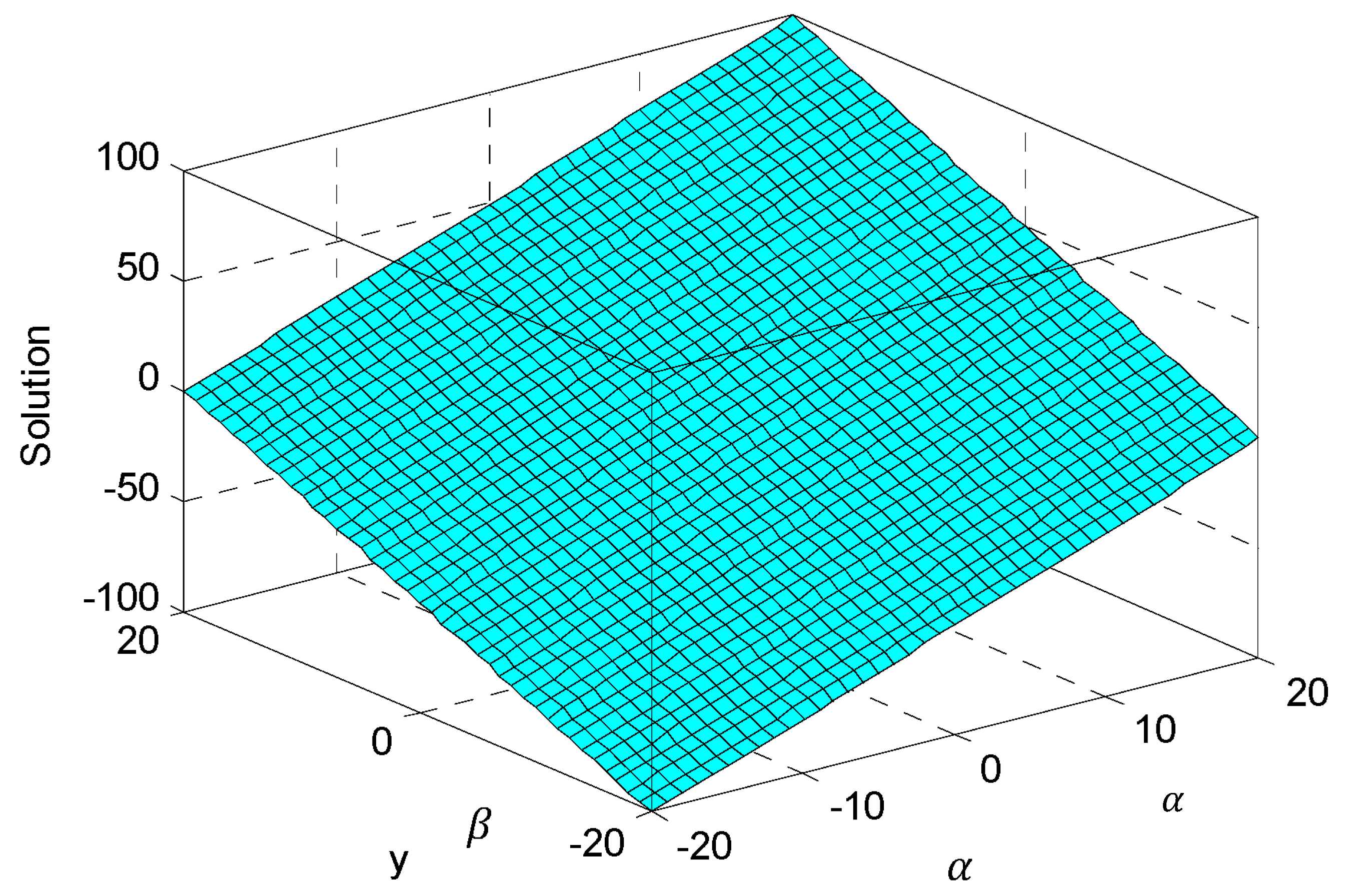
shows the comparison study of solutions obtained by new Laplace variation iteration method (up to fourth term), variational homotopy perturbation method (up to fourth term (as discussed in [1])), and the exact solutions for $\alpha =0.1, \beta =0.1$ and A = 2 of Example 1.

Table 2. The comparison of absolute errors obtained by new LVIM (up to fourth term) and VHPM (up to fourth term (as mentioned in [1])) for ($\alpha$, $\beta$) = (0.1, 0.1) and A = 2.

$\mathit{\tau }$	$\left|{\mathit{\phi }}_{\mathit{e}\mathit{x}\mathit{a}\mathit{c}\mathit{t}}-{\mathit{\phi }}_{\mathit{L}\mathit{V}\mathit{I}\mathit{M}}\right|$	$\left|{\mathit{\phi }}_{\mathit{e}\mathit{x}\mathit{a}\mathit{c}\mathit{t}}-{\mathit{\phi }}_{\mathit{V}\mathit{H}\mathit{P}\mathit{M}}\right|$ [1]
0.01	1.3604 × 10−9	4.0404 × 10−9
0.02	2.2210 × 10−8	6.5306 × 10−8
0.03	1.1475 × 10−7	3.3402 × 10−7
0.04	3.7016 × 10−7	1.0667 × 10−6
0.05	9.2255 × 10−7	2.6316 × 10−6
0.06	1.9531 × 10−6	5.5149 × 10−6
0.07	3.6948 × 10−6	1.0327 × 10−5
0.08	6.4373 × 10−6	1.7809 × 10−5
0.09	1.0532 × 10−5	2.8840 × 10−5
0.10	1.6399 × 10−5	4.4444 × 10−5

shows the comparison of absolute errors obtained by new Laplace variation iteration method (up to fourth term) and variational homotopy perturbation method (up to fourth term (as discussed in [1])) for $\alpha =0.1, \beta =0.1$ and A = 2 of Example 1.

Table 3. The comparison of absolute errors obtained by new LVIM (up to fourth term) and VHPM (up to fourth term (as mentioned in [1])) for ($\alpha$, $\beta$) = (0.1, 0.1) and A = 2 at different $\tau$.

$\mathit{\tau }$	Exact Solutions	$\left|{\mathit{\phi }}_{\mathit{e}\mathit{x}\mathit{a}\mathit{c}\mathit{t}}-{\mathit{\phi }}_{\mathit{L}\mathit{V}\mathit{I}\mathit{M}}\right|$	$\left|{\mathit{\phi }}_{\mathit{e}\mathit{x}\mathit{a}\mathit{c}\mathit{t}}-{\mathit{\phi }}_{\mathit{V}\mathit{H}\mathit{P}\mathit{M}}\right|$ [1]
0.2	0.50000000	3.2774 × 10−4	8.0000 × 10−4
0.3	0.57142857	2.1108 × 10−3	4.6286 × 10−3
0.4	0.66666666	8.6822 × 10−3	1.7067 × 10−2
0.5	0.80000000	2.8423 × 10−2	5.0000 × 10−2
0.6	1.00000000	8.2421 × 10−2	1.2960 × 10−1

shows the comparison of absolute errors obtained by new Laplace variation iteration method (up to fourth term) for different value of $\tau$. Figure 1 shows the physical behavior of solutions for $\tau =0.2$ at different domain of $\alpha$ and $\beta$.

Example 2. 

Consider the following (3+1)-D Burgers equation

$$\frac{\partial \phi \left(\alpha ,\beta ,z,t\right)}{\partial \tau }=\frac{1}{B}\phi \left(\alpha ,\beta ,z,\tau \right)\frac{\partial \phi \left(\alpha ,\beta ,z,\tau \right)}{\partial \alpha }+\frac{{\partial }^2\phi \left(\alpha ,\beta ,z,\tau \right)}{\partial {\alpha }^2}+\frac{{\partial }^2\phi \left(\alpha ,\beta ,z,\tau \right)}{\partial {\beta }^2}+\frac{{\partial }^2\phi \left(\alpha ,\beta ,z,\tau \right)}{\partial z^2}$$

(41)

with the initial conditions

$$\phi \left(\alpha ,\beta ,z,0\right)=B\left(\alpha +\beta +z\right)$$

By using the Laplace transformation on (41), we obtain

$$\begin{gathered} L\left\{\frac{\partial \phi \left(\alpha ,\beta ,z,\tau \right)}{\partial \tau }\right\}= L\left\{\frac{1}{B}\phi \left(\alpha ,\beta ,z,\tau \right)\frac{\partial \phi \left(\alpha ,v,z,\tau \right)}{\partial \alpha }+\frac{{\partial }^2\phi \left(\alpha ,\beta ,z,\tau \right)}{\partial {\alpha }^2}+\frac{{\partial }^2\phi \left(\alpha ,\beta ,z,\tau \right)}{\partial {\beta }^2}+\frac{{\partial }^2\phi \left(\alpha ,\beta ,z,\tau \right)}{\partial z^2}\right\} \\ sL\left\{\phi \left(\alpha ,\beta ,z,\tau \right)\right\}-\phi \left(\alpha ,\beta ,z,0\right) \\ =L\left\{\frac{1}{B}\phi \left(\alpha ,\beta ,z,\tau \right)\frac{\partial \phi \left(x,\beta ,z,\tau \right)}{\partial \alpha }+\frac{{\partial }^2\phi \left(\alpha ,\beta ,z,\tau \right)}{\partial {\alpha }^2}+\frac{{\partial }^2\phi \left(\alpha ,\beta ,z,\tau \right)}{\partial {\beta }^2}+\frac{{\partial }^2\phi \left(\alpha ,\beta ,z,\tau \right)}{\partial z^2}\right\} \\ sL\left\{\phi \left(\alpha ,\beta ,z,\tau \right)\right\}-\left(\alpha +\beta +z\right)\} \\ =L\left\{\frac{1}{B}\phi \left(\alpha ,\beta ,z,\tau \right)\frac{\partial \phi \left(\alpha ,\beta ,z,\tau \right)}{\partial \alpha }+\frac{{\partial }^2\phi \left(\alpha ,\beta ,z,\tau \right)}{\partial {\alpha }^2}+\frac{{\partial }^2\phi \left(\alpha ,\beta ,z,\tau \right)}{\partial {\beta }^2}+\frac{{\partial }^2\phi \left(\alpha ,\beta ,z,\tau \right)}{\partial z^2}\right\} \\ L\left\{\phi \left(\alpha ,\beta ,z,\tau \right)\right\}=\frac{B\left(\alpha +\beta +z\right)}{s}+ \\ \frac{1}{s} L\left\{\frac{1}{B}\phi \left(\alpha ,\beta ,z,\tau \right)\frac{\partial \phi \left(\alpha ,\beta ,z,t\right)}{\partial \alpha }+\frac{{\partial }^2\phi \left(\alpha ,\beta ,z,t\right)}{\partial {\alpha }^2}+\frac{{\partial }^2\phi \left(\alpha ,\beta ,z,t\right)}{\partial {\beta }^2}+\frac{{\partial }^{2}u\left(\alpha ,\beta ,z,t\right)}{\partial z^2}\right\} \end{gathered}$$

(42)

By the inverse Laplace transformation on (42), we obtain

$$\begin{array}{cc}\hfill \phi & =B\left(\alpha +\beta +z\right)+\hfill \\ & L^{-1}\left[\frac{1}{s} L\left\{\frac{1}{B}\phi \left(\alpha ,\beta ,z,\tau \right)\frac{\partial \phi \left(\alpha ,\beta ,z,\tau \right)}{\partial \alpha }+\frac{{\partial }^2\phi \left(\alpha ,\beta ,z,\tau \right)}{\partial x^2}+\frac{{\partial }^2\phi \left(\alpha ,\beta ,z,\tau \right)}{\partial {\beta }^2}+\frac{{\partial }^2\phi \left(\alpha ,\beta ,z,t\right)}{\partial z^2}\right\}\right]\hfill \end{array}$$

(43)

Using the modified variational iteration method from Equation (43), we obtain

$${\phi }_{m+1}=B\left(\alpha +\beta +z\right)+L^{-1}\left[\frac{1}{s} L\left\{{\phi }_m\frac{\partial {\phi }_m}{\partial x}+\frac{{\partial }^2{\phi }_m}{\partial x^2}+\frac{{\partial }^2{\phi }_m}{\partial {\beta }^2}+\frac{{\partial }^2{\phi }_m}{\partial z^2}\right\}\right]$$

(44)

From (44), we obtain

$${\phi }_0=B\left(\alpha +\beta +z\right),$$

$${\phi }_1=B\left(\alpha +\beta +z\right)\left(1+\tau \right),$$

$${\phi }_2=B\left(\alpha +\beta +z\right)\left(1+\tau +{\tau }^2+\frac{{\tau }^3}{3}\right),$$

$${\phi }_3=B\left(\alpha +\beta +z\right)\left(1+\tau +{\tau }^2+{\tau }^3+\frac{2{\tau }^4}{3}+\frac{{\tau }^5}{3}+\frac{{\tau }^6}{9}+\frac{{\tau }^7}{63}\right),$$

The solution can be obtained by

$$\phi =\underset{m\to \infty }{\lim }{\phi }_m$$

Now, after simplification, we obtain

$$\phi =B\left(\alpha +\beta +z\right)\left(1+\tau +{\tau }^2+{\tau }^3+{\tau }^4+{\tau }^5\dots \right)$$

This implies

$$\phi =B\left(\alpha +\beta +z\right){\left(1-\tau \right)}^{-1}$$

or

$$\phi =\frac{B\left(\alpha +\beta +z\right)}{\left(1-\tau \right)}$$

This series solution is valid only if  $\left|\tau \right|<1$.

Table 4. The comparison of new LVIM (up to fourth term), VHPM (up to fourth term (as mentioned in [1])), and exact solution for ($\alpha$, $\beta$, z) = (0.1, 0.1, 0.1) and B = 3.

$\mathit{\tau }$	Exact	NLVIM	VHPM [1]
0.01	0.90909090	0.90909090	0.90909090
0.02	0.91836734	0.91836729	0.91836720
0.03	0.92783505	0.92783479	0.92783430
0.04	0.93750000	0.93749916	0.93749760
0.05	0.94736842	0.94736634	0.94736250
0.06	0.95744680	0.95744241	0.95743440
0.07	0.96774193	0.96773362	0.96771870
0.08	0.97826086	0.97824638	0.97822080
0.09	0.98901098	0.98898729	0.98894610
0.10	1.00000000	0.99996310	0.99990000

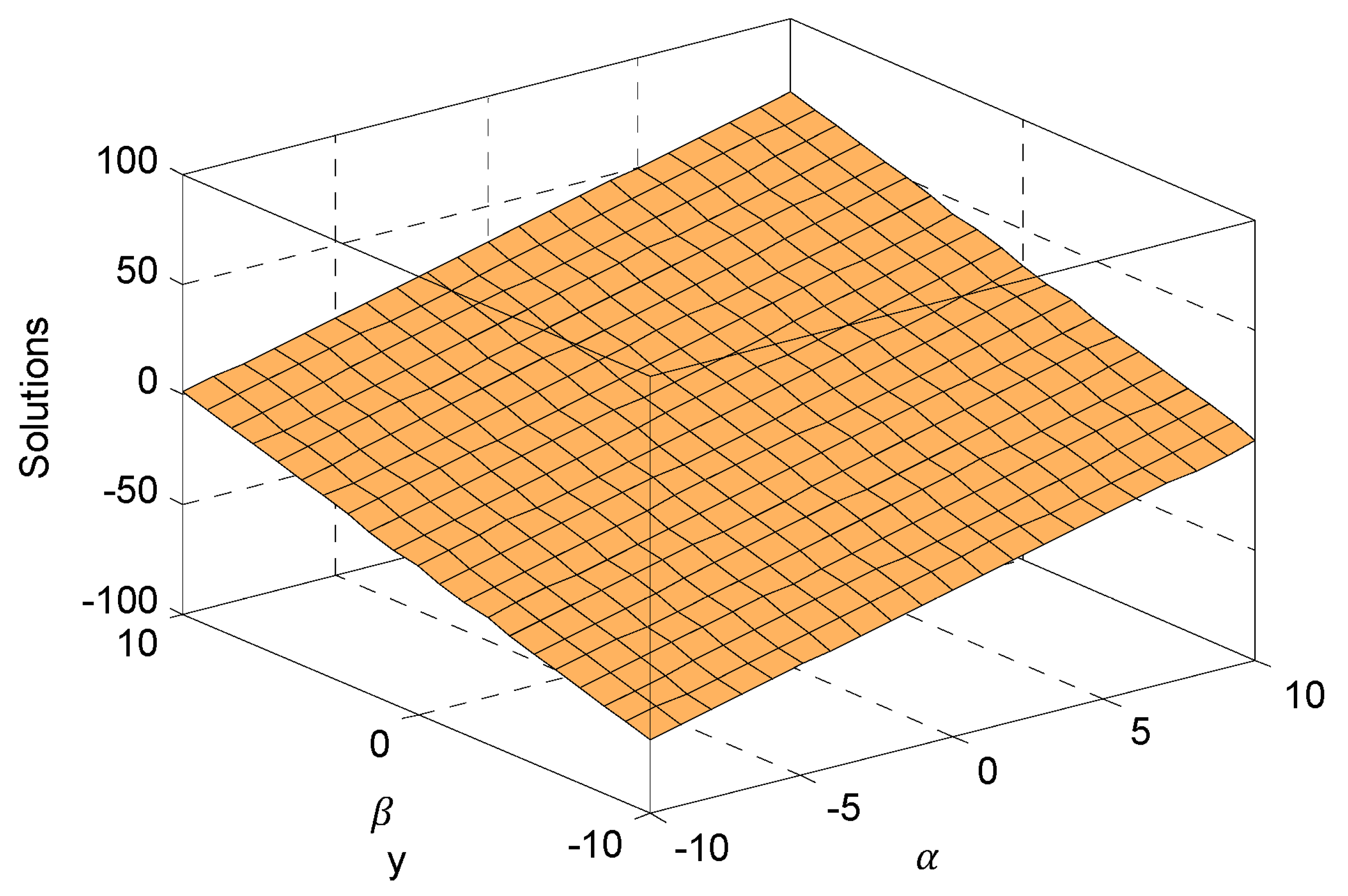
shows the comparison study of solutions obtained by new Laplace variation iteration method (up to fourth term), variational homotopy perturbation method (up to fourth term (as discussed in [1])), and the exact solutions for $\alpha =0.1, \beta =0.1, z=0.1$ and B = 3 of Example 2.

Table 5. The comparison of absolute errors obtained by new LVIM (up to fourth term) and VHPM (up to fourth term (as mentioned in [1])) for ($\alpha$, $\beta$, z) = (0.1, 0.1, 0.1) and B = 3.

$\mathit{\tau }$	$\left|{\mathit{\phi }}_{\mathit{e}\mathit{x}\mathit{a}\mathit{c}\mathit{t}}-{\mathit{\phi }}_{\mathit{L}\mathit{V}\mathit{I}\mathit{M}}\right|$	$\left|{\mathit{\phi }}_{\mathit{e}\mathit{x}\mathit{a}\mathit{c}\mathit{t}}-{\mathit{\phi }}_{\mathit{V}\mathit{H}\mathit{P}\mathit{M}}\right|$ [1]
0.01	3.0608 × 10−9	9.0909 × 10−9
0.02	4.9972 × 10−8	1.4694 × 10−7
0.03	2.5818 × 10−7	7.5155 × 10−7
0.04	8.3287 × 10−7	2.4000 × 10−6
0.05	2.0757 × 10−6	5.9211 × 10−6
0.06	4.3945 × 10−6	1.2409 × 10−5
0.07	8.3134 × 10−6	2.3235 × 10−5
0.08	1.4484 × 10−5	4.0070 × 10−5
0.09	2.3698 × 10−5	6.4889 × 10−5
0.10	3.6899 × 10−5	1.0000 × 10−4

shows the comparison of absolute errors obtained by new Laplace variation iteration method (up to fourth term) and variational homotopy perturbation method (up to fourth term (as discussed in [1])) for particular values of variables $\alpha =0.1, \beta =0.1, z=0.1$ and B = 3 of Example 3.

Table 6. The comparison of absolute errors obtained by new LVIM (up to fourth term) and VHPM (up to fourth term (as mentioned in [1])) for ($\alpha$, $\beta$, z) = (0.1, 0.1, 0.1) and B = 3 at different $\tau$.

$\mathit{\tau }$	Exact Solutions	$\left|{\mathit{\phi }}_{\mathit{e}\mathit{x}\mathit{a}\mathit{c}\mathit{t}}-{\mathit{\phi }}_{\mathit{L}\mathit{V}\mathit{I}\mathit{M}}\right|$	$\left|{\mathit{\phi }}_{\mathit{e}\mathit{x}\mathit{a}\mathit{c}\mathit{t}}-{\mathit{\phi }}_{\mathit{V}\mathit{H}\mathit{P}\mathit{M}}\right|$ [1]
0.2	1.12500000	7.3742 × 10−4	1.8000 × 10−3
0.3	1.28571428	4.7493 × 10−3	1.0414 × 10−2
0.4	1.50000000	1.9535 × 10−2	3.8400 × 10−2
0.5	1.80000000	6.3951 × 10−2	1.1250 × 10−1
0.6	2.25000000	1.8545 × 10−1	2.9160 × 10−1

shows the comparison of absolute errors obtained by new Laplace variation iteration method (up to fourth term) for different value of $\tau$. Figure 2 shows the physical behavior of solutions for $\tau =0.1$ at different domain of $\alpha , \beta$ and $z$.

4. Conclusions

Based on the preceding discussion and experiments, the combination of the Laplace transforms, and the variational iteration technique presents an effective approach to solve the (2+1)-D and (3+1)-D Burgers equations. Compared to the variational homotopy perturbation technique (VHPM), the new Laplace variational iteration method (LVIM) is more effective in obtaining an approximate solution that closely approximates the actual one. It is possible that this technique may be utilized in the future to solve the three-dimensional Burgers equation system.