An Improved Sparrow Search Algorithm for Global Optimization with Customization-Based Mechanism

Abstract

To solve the problems of the original sparrow search algorithm’s poor ability to jump out of local extremes and its insufficient ability to achieve global optimization, this paper simulates the different learning forms of students in each ranking segment in the class and proposes a customized learning method (CLSSA) based on multi-role thinking. Firstly, cube chaos mapping is introduced in the initialization stage to increase the inherent randomness and rationality of the distribution. Then, an improved spiral predation mechanism is proposed for acquiring better exploitation. Moreover, a customized learning strategy is designed after the follower phase to balance exploration and exploitation. A boundary processing mechanism based on the full utilization of important location information is used to improve the rationality of boundary processing. The CLSSA is tested on 21 benchmark optimization problems, and its robustness is verified on 12 high-dimensional functions. In addition, comprehensive search capability is further proven on the CEC2017 test functions, and an intuitive ranking is given by Friedman's statistical results. Finally, three benchmark engineering optimization problems are utilized to verify the effectiveness of the CLSSA in solving practical problems. The comparative analysis shows that the CLSSA can significantly improve the quality of the solution and can be considered an excellent SSA variant.

1. Introduction

Due to the continuous development of industry and technology, various fields have developed rapidly, accompanied by the emergence of many complex optimization problems. The key to solving these problems is to input variables that meet the conditions in the given search space to obtain the optimal feasible solution. Specifically, these types of optimization problems generally have three main elements: decision variables, objective functions, and constraints. Among them, the decision variable indicates the variable that the problem needs to be solved, the objective function is the main object of maximization or minimization, and the constraints are often divided into equality constraints and inequality constraints. In summary, it can be seen that the general form of this type of problem is:

$$\begin{array}{c}\min f(x)\\ x=(x_1,x_2,\dots ,x_n)\in R\end{array}$$

(1)

$$\begin{array}{cc}\hfill s.t.& c_i\left(x\right)\le 0,i=1,2,\dots ,m\hfill \\ & c_i\left(x\right)=0,i=m+1,\dots ,m+l\hfill \end{array}$$

(2)

where Equation (1) represents the minimization objective function. $R$ represents the entire search space. Equation (2) represents the constraints, including m inequalities and l equations.

The traditional approach to solving such problems is based on mathematical analysis. Researchers tend to choose solution methods flexibly according to the characteristics of the problems. For unconstrained optimization problems with a differentiable objective function, gradient and Newton methods are better choices [1]. For constrained optimization problems, methods based on the Lagrange multiplier are appropriate. Moreover, the differentiability and directional differentiability of the objective function [2], whether the constraints are linear or not, and whether the feasible domain is continuous or not are all important references for choosing the corresponding algorithms. It can be seen that the traditional methods have more limitations, which are not conducive to generalization to more problems and are no longer able to meet the high efficiency required by technological developments in terms of both time and accuracy. Due to the urgent need to solve real problems, optimization methods different from traditional exact algorithms have drawn much attention from the academic community. Consider that the solution space of most real-world problems is infinite, or it is too costly to evaluate all solutions with full coverage. Therefore, it makes sense to obtain a good solution within an acceptable time [3]. Based on computational intelligence mechanisms, researchers have explored multiple perspectives and pioneered a series of feasible methods to tackle the technical challenges of optimization, called metaheuristic algorithms or intelligent optimization algorithms. Since this type of method does not have any special requirements for the objective function and is not limited to solving specific problems, it has gradually become a hotspot in optimization research.

Exploring sources of inspiration for the development of such algorithms, there are five different groups in which the existing metaheuristics can be evaluated: evolution-based [4,5], physics-based [6,7,8], social-based [9,10], swarm-based [11,12,13,14], and other laws of nature [15,16,17]. The fourth category is better known for research and has given birth to the largest number of algorithms [18]. Swarm-based metaheuristics are inspired by foraging [19,20], hunting [21,22], and various other behaviors. With the depth of research, researchers used to call this category of algorithms swarm intelligence optimization algorithms. It is worth clarifying that the Ant Colony System (ACS) [11], proposed in 1991, and the Particle Swarm Optimization algorithm (PSO) [12,13], introduced in 1995, are two creations that led the research boom in this direction. In the last decade, new swarm intelligence algorithms have emerged, with researchers mimicking the behavior of various animals for modeling and naming the proposed optimization algorithms according to various animals’ names. The latest ones include the Lion Swarm Optimization algorithm (LSO) [23] in 2018, the Butterfly Optimization Algorithm (BOA) [24] in 2019, Harris Hawk Optimization (HHO) [25], the Chimp Optimization Algorithm (CHOA) [26] in 2020, etc. Compared with traditional optimization methods, these swarm-based algorithms have the advantages of fewer parameters, shorter running time, and simpler experimental operations. In today’s nonlinear and multi-modal optimization-seeking problems, swarm intelligence algorithms present excellent merit-seeking ability and feasibility.

Although the expectations of optimization problems are essentially the same, different algorithms are only capable of showing a strong performance in a fraction of optimization problems. Therefore, new optimization algorithms need to be continuously proposed and applied to different sets of problems. Through extensive research and experimental analysis, valuable ideas are proposed to eventually find commonalities in optimization. This is what the No Free Lunch Theorem has taught us [27].

In 2020, Xue et al. [28] proposed the Sparrow Search Algorithm (SSA), a novel swarm-based creation. This algorithm is implemented with less difficulty, has better self-organization ability, and demonstrates better global exploration and local mining ability in a complete predation process. However, the excessive speed of the search causes the algorithm to tend to converge too quickly in the process of finding the optimal solution and overshoot into a stagnant state, which not only loses the diversity of the population but also affects the convergence to a larger extent.

Researchers have made many attempts to solve these problems. Lv et al. [29] combined tent chaotic sequences and Gaussian variation strategy to propose an improved CSSA, where chaotic perturbation of local individuals is beneficial in solving the problem of falling into local optima. Wang et al. [30] proposed more than one learning strategy to update the best and worst position information, respectively. In addition, the improved longitudinal interleaving mechanism is fused in the update phase of followers to further balance the search capability of the algorithm. Yan et al. [31] subdivided the follower phase into two phases, global search and local search. A variable spiral factor and an improved iterative search strategy were added to each of the two stages. The effect of the improved strategy was verified using the variation in the number of individuals outside the boundary. Gad et al. [32] proposed a strategy for 3RA and local search algorithm incorporated into the original SSA in order to solve the problem that the original SSA lacked proper stimulus search in the feasible region and, thus, caused significant stagnation in the development process. A comparison was made with competing algorithms for the classification feature selection problem to demonstrate the superiority of the improvement. Yang et al. [33] utilized good point set initialization and then combined the game predatory mechanism and suicide mechanism into the SSA to improve the merit-seeking performance and improve the existing diversity index evaluation for the shortcomings of the existing SSA, which effectively avoids the defects caused by invalid search.

In addition to improvements in the underlying algorithm, validation of the algorithm for specific applications has received increasing attention. Zhou et al. [34] attempted to incorporate crossover and variation operations in the scout update phase of the SSA and combined a series of improvements in the controlled segment phase values to make it better for application in noisy natural environments. In experiments, the newly proposed strategy proved to be superior to the proposed wavefront shaping focusing algorithm in different noisy environments by representing the individual sparrow and its fitness value as a phase mask and the corresponding enhancement, respectively. Wang et al. [35] constructed a chaotic SSA based on Bernoulli mapping, Corsi variance, and dynamic adaptive weighting strategies that reduced the operating cost of microgrid cluster systems. Zhu et al. [36] utilized an adaptive SSA to optimize the model parameters of a proton exchange membrane fuel cell (PEMFC) and parametrically minimized the sum of squared errors (SSE) between empirical and computed stack voltages. The improved ASSA was experimentally demonstrated to have high efficiency in optimizing the performance. Tian et al. [37] combined the improved im-SSA with sequential quadratic programming to achieve a reduction in system fuel cost and built a hybrid generation system based on it to contribute to the supply of electricity in remote areas. Wu et al. [38] adopted sinusoidal mapping, hyperparameter adaptive tuning, and variational strategies to improve the SSA. The number of hidden layer nodes in the random configuration network was generated according to the above strategies, and the parameters in the fast random configuration network were optimized to improve the performance of classification. Fan Y et al. [39] combined the SSA and PSO organically and designed a new method using the advantages of each of the two models, which was successfully applied to the hyperparameter optimization of neural networks. This method avoids the deficiency of data overflow caused by the SSA and achieves an effective reduction in minimum error. In addition, Zhang Z et al. [40] improved the SSA as applied to optimal trajectory solving for robots to ensure smooth paths and less time overhead. Chen et al. improved the SSA to implement image segmentation [41], and Yin et al. [42] applied the ISSA to DV-hop localization to obtain satisfactory localization accuracy.

Although the SSA has been proposed for a relatively short period of time, the number of publications with the SSA as the object of research has grown at an explosive rate and shown a stable trend [43]. From the existing studies, it is easy to see that the improved algorithm only performs well in some of the tested functions, and the too-fast convergence rate often leads to a premature loss of population diversity. In the basic SSA, the population is initialized with a random distribution, which leads to problems such as irrational distribution of the algorithm, reduced diversity, and a certain blindness in the search for individuals. Secondly, the original algorithm has limited merit-seeking ability, and its convergence accuracy needs to be improved. Further, in the original follower update strategy, the setting of a poorly positioned sparrow jumping directly out of the current position cannot effectively use the information around that position. Finally, the original boundary processing mechanism is too simple to take into account the direction and step length of position update, which lacks rationality.

In view of the above ideas of improvement strategies and thinking about the existing optimization algorithms, this paper proposes a CLSSA based on the idea of customization for optimization in the global context that helps solve the defects, including insufficient optimization precision and falling into local optimality easily. The points of innovation can be summed up as follows.

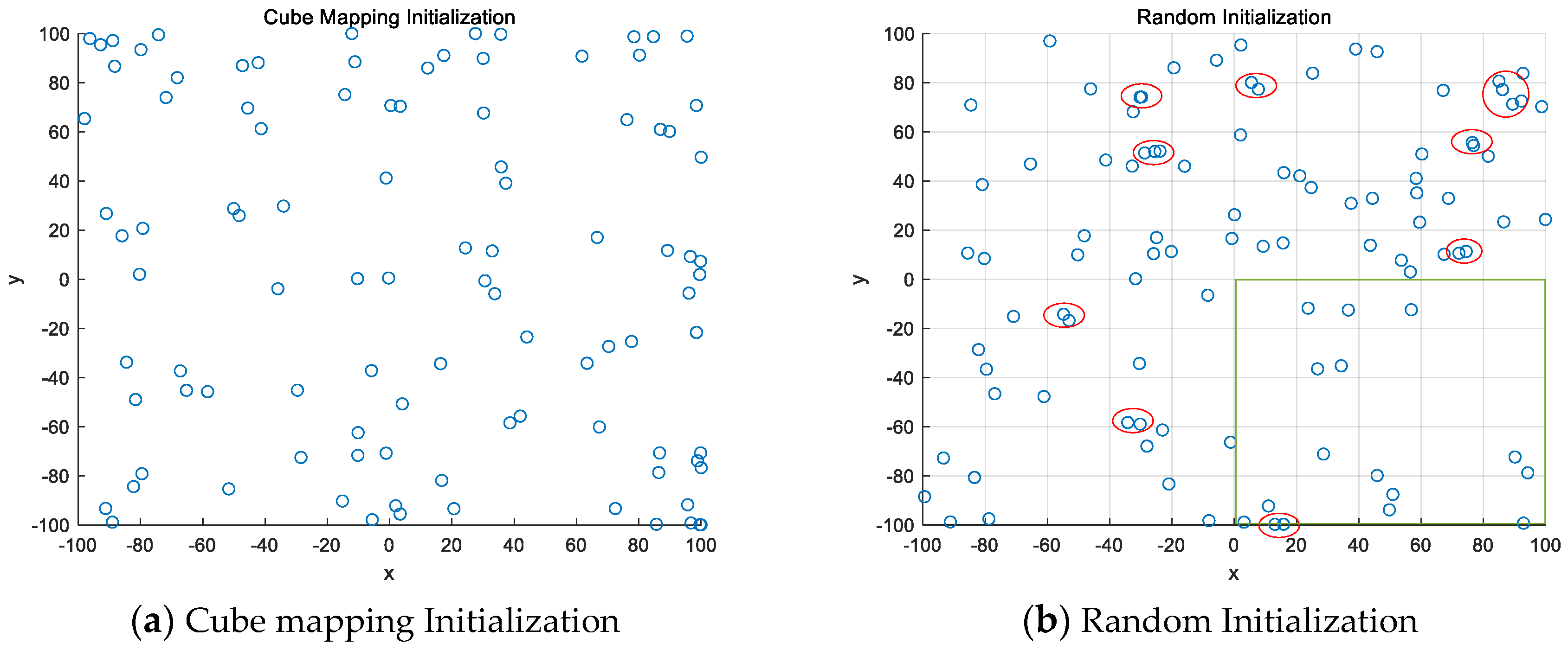
• By utilizing cube mapping to initialize the population, the inherent randomness of chaos and the irregular orderliness are exploited to make the initial population state dispersion more reasonable.
• By introducing the adaptive spiral predation mechanism to change the predation mechanism of followers, better exploitation is accomplished.
• For position updating of sparrows with different search abilities in the whole population, a novel customized learning strategy is proposed. The combination of this strategy makes full use of essential positional information and achieves a balance between exploration and exploitation.
• In view of the different abilities and division of labor of the three roles, a novel boundary processing mechanism is proposed to improve the rationality of boundary processing, which effectively avoids the accumulation of the population on the boundary, thus increasing the population diversity.
• The feasibility of the CLSSA in engineering optimization is verified with three classical discrete engineering optimization problems.

In this work, in accordance with a certain logical order, the first section introduces the swarm intelligence algorithm and the current research status of the SSA, as well as the research background of this paper. Section 2 introduces the original SSA. In Section 3, the innovations of this paper are introduced, and the CLSSA is described in detail. Multiple sets of experiments are set up to verify the merit-seeking performance and robustness of the CLSSA in Section 4. Then, in Section 5, the CLSSA is applied to three classical discrete engineering optimization problems, and the feasibility and effectiveness of the proposed algorithm are further demonstrated using the obtained data. Finally, a concise conclusion of this paper is given in Section 6.

2. Sparrow Search Algorithm

The SSA, as a novel swarm-based algorithm, simulates the mechanisms of teamwork, information exchange, and anti-feeding in sparrow populations during foraging. The bionic principle consists of dividing the whole population into three parts: discoverer, follower, and scouter. The discoverer, as the best-positioned individual in the current population, is responsible for leading the entire group in foraging, while the rest of the sparrows, called followers, follow the discoverer. They always stay competitive with the discoverer for ownership of the food resources. In other words, the roles of discoverers and followers can be interchanged while the overall ratio remains the same [30]. In particular, it is emphasized that the discoverers search more widely than the followers, while the follower’s search is relatively limited and localized [44]. In addition to the above two roles, the third role, scouter, is set according to a certain percentage with the responsibility of alerting the appearance of natural enemies and the occurrence of various dangers. In order to evaluate the position of the individual and their own ability, the index of fitness value is introduced as the basis of evaluation, which means the closer the fitness value is to the optimum zero, the heavier the predation ability. The above process is divided into three main steps for position updating.

When there is no danger, the discoverer leads the population to search widely. Conversely, when danger appears and the alarm value exceeds the safety threshold (ST), the strategy is to quickly approach the safe position. The updated formula is as follows.

$$x_{i,j}^{t+1}=\left\{\begin{array}{c}{x}_{i,j}^t·\exp (\frac{-i}{\alpha ·T}) if R_2<ST\\ x_{i,j}^t+Q·L if R_2\ge ST\end{array}\right.$$

(3)

where $x_{i,j}^t$ denotes the position, its superscript $t$ denotes the number of iterations, while the subscript $i$ denotes the individual serial number, and j denotes the number of dimensions. When the superscript changes to $t+1$, it means the update is complete. T denotes the upper limit for iterating. $\alpha$ is a uniform number that meets $\left(0,1\right]$. $Q$ is a random number that obeys the standard normal distribution. $L$ is a matrix of all ones. Alarm value $R_2\in \left[0,1\right]$ and $ST\in \left[0.5,1\right]$.

For the followers, the lower-ranked ones choose to leave the current location and search a more distant place for foraging, while the sparrows in the top position will choose to forage around the best location found by the finder. The mechanism can be described as:

$$x_{i,j}^{t+1}=\left\{\begin{array}{cc}Q·\exp (\frac{x_{w,j}^t-x_{i,j}^t}{i^2})\hfill & if i>N/2\hfill \\ x_P^{t+1}+\left|x_{i,j}^t-x_p^{t+1}\right|·A^{+}·L\hfill & otherwise\hfill \end{array}\right.$$

(4)

where $x_w$ and $x_p$ denote the current global worst position and the current global optimum of the j-dimension, respectively. $A$, a matrix of $1\times d$ is randomly assigned −1 or +1. $A^{+}$ satisfies $A^{+}=A^T{(A{A}^T)}^{-1}$. The lower-ranked follower corresponds to the part of $i>N/2$, while the other part is updated in a different way.

The scout mechanism is a more specific presence in the SSA, which usually requires 10–20% of the overall individuals to play the role of scouts. When scouts take up their position at the periphery of the population, moving to the optimal position when encountering danger is a necessary choice. Meanwhile, scouts in the middle of the population will choose to move closer to others to reduce the possibility of being attacked themselves when realizing the danger. The scout position updated formula is as follows.

$$x_{i,j}^{t+1}=\left\{\begin{array}{c}{x}_{i,j}^t+\beta \left|x_{i,j}^t-x_{b,j}^t\right|, f_i\ne f_g\\ x_{i,j}^t+K\frac{x_{i,j}^t-x_{w,j}^t}{\left(f_i-f_w\right)+\epsilon }, f_i=f_g\end{array}\right.$$

(5)

where $\beta$ is a random number with the same distribution as $Q$. $K$ is a random number within $\left[-1,1\right]$. $f_i$, $f_g$ and $f_w$ denote three important fitness value, the current sparrow’s fitness, the global optimum, and the global worst fitness values, respectively. $\epsilon$ is an infinitesimal constant to avoid zero-division-error.

3. CLSSA

3.1. Cube Chaos Mapping Initialization Population

In the original SSA, as in the majority of swarm intelligence algorithms, the rand () function is utilized to randomly generate quantitative random numbers between 0 and 1 and then carrier to the desired interval to obtain the initial population location. Obviously, the initial positions obtained by this method can guarantee randomness, but there are problems such as local aggregation and uneven distribution, which will bring problems such as slow convergence and premature loss of diversity to the following search. In light of the better global ergodicity and randomness of chaos, chaotic sequences have been implemented in many metaheuristic algorithms [45] whose roles can be divided into replacing random variables and initializing populations [46]. With the proposal of the sparrow search algorithm, tent mapping [29], logistic mapping [41], and ICMIC mapping [30] have been employed by researchers to improve the problem of the poor initialization effect of sparrow populations. The good results brought by the above strategy are reflected in the experimental data.

Cube chaos mapping (cube for short) is a one-dimensional self-mapping, which is more chaotic than the commonly used finite fold number mapping, and the distribution is more uniform than logistic mapping [47]. In this paper, cube is chosen to replace the pseudo-random number generator. The initial position of the population is generated by an iterative method until a predetermined sparrow member is reached [45]. Its necessary steps are as follows:

• A d-dimensional vector is randomly generated, the process is denoted as $\mathrm{y}=\left\{y_1,y_2,\dots ,y_d\right\}$, each dimension satisfies $y_i\in \left[-1,1\right],y=1,2,\dots d$, and y is used to denote the first individual position.
• A new d-dimensional vector is generated using Equation (6).

  $$y_{i+1}=4y_i^3-3y_i$$

  (6)
• The values of Equation (6) are brought into Equation (7) to obtain the values of each dimension of the individual.

  $$x_i=lb+\frac{\left(ub-lb\right)\left(y_i+1\right)}{2}$$

  (7)

  where $ub$ and $lb$ denote the lower and upper bounds of the search interval, respectively.
• Individual positions were obtained as:

  $$x=\left\{x_1,x_1,\dots ,x_d\right\}$$

  (8)

Figure 1 shows the distribution of sparrow populations in two-dimensional space after initializing the populations with random initialization and cube initialization, respectively, in the initialization phase, where each dot represents an individual sparrow. In order to prove the fairness, both methods set the population size at 100 and choose the same test function for testing. It can be observed in Figure 1a that the overall dispersion performs well, and there is no aggregation of most individuals. In contrast, as seen in Figure 1b, the distribution of individuals after random initialization has a higher number of individuals with overlapping positions (marked by red ovals). In addition, after dividing the whole two-dimensional space into four equal areas, it is easy to see that the number of individuals in the lower-right area (marked by a green box) in Figure 1b is significantly less than that in the other areas. The above situation does not occur in Figure 1a. In summary, it can be seen that cube initialization provides assistance in increasing the diversity and rationality of the population distribution during the initialization phase. In Section 4.1, several types of chaos mentioned in the first paragraph of this section are compared to further demonstrate the superiority of cube initialization through relevant data.

3.2. Adaptive Spiral Predation

In the original SSA, poor-position followers increase their foraging odds by tuning directly away from the current area, which obviously reduces the search and utilization of locations near the current location. Meanwhile, in view of the fact that multiple-example learning in customized learning is capable of achieving escape from poorer locations, the search method of poorer followers in this paper will be altered to increase the contribution of sparrows in this part. It is considered that a whale population will form a bubble net to attack prey by spiraling away after finding the prey, which can reduce the surroundings and complete the hunt. In the WOA [48], Mirjalili S utilized the idea of spiral predation to describe the process and obtained superior search results. The following equation is proposed after combining the above idea with the original strategy.

$$\begin{array}{l}a=-1+t\times \left(\left(-1\right)÷T\right)\\ l=\left(a-1\right)\times rand+1\end{array}$$

(9)

$$x_{i,j}^{t+1}=\cos \left(l\times \pi \right)\times \exp \left(\frac{x_w^t-x_{i,j}^t}{i^2}\right),i>\frac{N}{2}$$

(10)

where $a$ is the adaptive coefficient, $l$ is the parameter of spiral control, and the other parameters are the same as in Section 2.

3.3. Customized Learning

A learning mechanism is a method of information transfer proposed to simulate the knowledge transfer method in people’s daily life. Predetermined position or velocity information is assigned to other individuals or vectors, and thus, a transformation is performed on that individual or vector. The most well-known learning mechanism is opposition learning [49], followed by general opposition-based learning [50], competitive learning [51], lens learning [52], and so on. As the study progressed, the researchers found that a single learning mechanism could ignore the differences among individuals in the population to some extent. For individuals ranked at different stages in the population, using different strategies for updating can achieve higher convergence.

For the above problems, new combinatorial mechanisms have been proposed, such as Ouyang et al., who proposed simultaneous updating of optimal and worst positions [53]. Zhang et al. proposed a three-learning strategy [54], which reduced the running time and obtained better results. Xia et al. [55] chose different learning situations according to the size of the three solutions to obtain excellent solutions. Inspired by these articles, a customized learning strategy based on the student tutoring mechanism in school classes is proposed in this paper, which gives differentiated management and guidance for different types of students.

Usually, students in a class have different levels of learning abilities. The most intuitive reflection of learning ability is test scores. The students who rank in the top 10% in each exam are called Elite and are considered to have the best mastery of that level of knowledge and the best learning skills. These students are often chosen as the learning objects for their excellent grades. On the contrary, the bottom 10% of the class, called Learner, is considered to have the worst learning ability and needs supervision and support. The rest of the students who also rank in the top half of the grade range are often considered to have a better attitude toward learning and can manage their study tasks better. These students are trusted by teachers with their self-learning ability. Some students who are in the 50–90% range are considered to have a high potential for improvement; however, they fail to show it in their grades due to poor learning methods and other reasons. These students receive the most attention from their teachers and are called Potential.

By combining the descriptions above, the entire class can be divided into four groups according to the ranking of their grades after each test, as shown in Figure 2. In addition, a novel customization-based learning strategy is proposed in this paper. For all students except Elite, corresponding study plans are developed separately to help them progress and achieve the effect of improving their grades.

3.3.1. Elite–Learner Paired Learning

Learners, who ranked in the bottom 10% of the class, were assigned one-on-one help with the Elites, who ranked in the top 10%, as a measure to monitor their learning. Research has shown that paired learning, according to the principle of ranking pairs, maximizes the effect of help [56]. The principle is that two groups of equal numbers of students are ranked according to their test scores. In this case, the Elite group is referred to as ES. The students in the Elite group are noted as $x_i^E$, the Learner group is referred to as LS, and the poor students are noted as $x_i^L$. As shown in Figure 3, both groups have $M/2$ individuals and satisfy:

$$\forall x_i^E\in ES and \forall x_i^L\in LS, f\left(x_i^E\right)<f\left(x_i^L\right)$$

(11)

$$f\left(x_i^E\right)<f\left(x_{i+1}^E\right) and f\left(x_i^L\right)<f\left(x_{i+1}^L\right), i=1,2,\dots ,M/2$$

(12)

$$x_1^L\to x_1^E\dots x_{M/2}^L\to x_{M/2}^E$$

(13)

The specific Elite–Learner Paired Learning Strategy for each poor student to consult with an elite individual of the same rank in the elite group is as follows.

$${x^{\prime }}_i^L=x_i^L+\lambda \left(x_i^E-x_i^L\right)$$

(14)

where ${x^{\prime }}_i^L$ denotes the position obtained after learning and $\lambda$ denotes a random number with the same distribution as $Q$ above.

3.3.2. Selected Learning

Selected students, who ranked in the 10–50% range, are considered to have excellent self-learning ability, and no compulsory help will be given. They may choose whether to consult the best students according to their own judgment and decide whether to keep the learning results according to the greed principle after consulting. This type of learning is called Selected learning. To simulate this selection, a selection threshold $S$ and a random $R$ conforming to the standard normal distribution are introduced. After comparing the above two, if the random number exceeds the threshold, the learning process is executed; otherwise, it is not executed. Analogously to the sparrow population, $x$ denotes the individual position, and the position updated formula is as follows.

$${x^{\prime }}_{{}_i}^t=\left\{\begin{array}{cc}{\omega }_i{x}_i^t+{\omega }_b{x}_b^t& ,S\le R\hfill \\ x_{{}_i}^t& ,S\ge R\hfill \end{array}\right\}$$

(15)

where $x_i^t$ denotes the current individual position, $x_b^t$ denotes the current global superior position, ${\omega }_i$ and ${\omega }_b$ denote the weight coefficient of the current individual position and the optimal position, respectively.

$$\left\{\begin{array}{c}{\omega }_i=\frac{f(i)}{f(i)+f(b)}\\ {\omega }_b=\frac{f(b)}{f(i)+f(b)}\end{array}\right.$$

(16)

where $f(i)$ and $f(b)$ denote the fitness value of the current individual and the current global optimum, respectively.

The dynamic adjustment of the weight coefficients according to the fitness value is closer to the actual situation. At the same time, it can avoid the dominance of the current global optimal position information, thus leading the whole population to gather near the current optimal and effectively avoiding the potential risk of falling into premature maturity. In addition, the greedy principle is added after the position update, and the strategy simulates the process of judging the results by this part of students after consulting excellent students, emphasizing that the students in this ranking have better self-learning ability and self-consciousness.

3.3.3. Multi-Example Learning

For students ranked in the 50–90% range with greater potential for improvement, it is a good choice to make progress by combining elite help and self-consultation with students who are better than themselves. The specific strategy is finding a random role model in each of the Elite and Selected groups to emulate and improving by combining their own study methods with those of the highest-performing students. This kind of learning method that combines learning from many students who are better than themselves and their own efforts is called multi-example learning. Applied to sparrow populations, a center-of-mass variation strategy is introduced. Using random elite individuals $x_m^E(t)$, random selected individuals $x_n^S(t)$, their own position $x_i(t)$, and the current optimal individual position $x_b(t)$ together to form a new position ${x^{\prime }}_i(t)$.

$${x^{\prime }}_i(t)=rand·\left(\frac{x_m^E(t)+x_n^S(t)+x_i(t)}{3}-x_b(t)\right)+x_b(t)$$

(17)

Combining the above customized learning strategies into the location update of the sparrow population, the students in the class are analogized to the sparrows in the sparrow population, the academic performance is analogized to the fitness value of the location, the change in academic performance is analogized to the location update, and each test is analogized to each iteration of the sparrow. As can be seen, in contrast with traditional learning strategies, a customized learning strategy is able to generate personalized learning methods according to the different situations of each part. Just as in a class where the teacher cannot dogmatically use the same teaching method for students with different learning abilities, multiple strategies in a sparrow population contribute to a progressive search for the entire population while retaining good positions.

3.4. Customized Learning

The boundary processing strategy is one of the important methods to preserve the diversity of the population by redefining the positions of individuals beyond the boundaries so that the population outside the effective positions can return to the previously predefined search space. A uniform boundary treatment is adopted in the original SSA by defining individuals outside the maximum boundary on the uppermost boundary and, similarly, defining individuals below the minimum boundary on the lower boundary.

There is no doubt that such a uniform and simple treatment mechanism will cause the phenomenon of local aggregation on the search boundary. Although preserving the population size to some extent, it also has the drawback of losing diversity. At the same time, the difficulty of the next optimization will be increased, which will affect the expected results. Experimental evidence of this point will be given in Section 4. In view of the variability of the three stages in the SSA, this paper proposes a novel multi-strategy boundary processing method, which makes full use of the targeted processing corresponding to the purpose of different stages, respectively.

In the discoverer stage, the whole population should be committed to finding new food, and the current optimum is potentially the most suitable foraging site. However, the initial stage of foraging is accompanied by the uncertainty of the optimal location, so the boundary processing of individuals should retain randomness to a certain degree. Similarly, after the vigilantes are updated, the beginning of the next iteration will follow immediately. The more dispersed the initialized population is, the higher the probability that the optimal solution can be obtained after the corresponding stage of the strategy is carried out. The boundary processing method, accompanied by strong randomness, gives the population the ability to jump out of the local optimum with a certain chance. The boundary processing method with updated discoverer and scout positions is given below.

$$x_i^{\text{'}}=ub-\left(ub-lb\right)·rand, x>ub \mathrm{or} x<lb$$

(18)

In the follower phase, the competition is the most intense due to the highest number of sparrows in this part. As a result, potential individuals beyond the boundary reach the highest number of all three phases [31]. Throughout the SSA, the core purpose of the discoverer update phase is to find the superior global optimization position, while the follower phase is to randomly wander around the previously found position and attempt to exploit it in depth. In the original follower mechanism, the well-adapted followers have moved to the vicinity of the superior global optimization position, ensuring the search of the potentially optimal region. Therefore, the treatment of individuals beyond the boundaries in this phase should also be developed around the current optimal position.

Considering the original SSA, the update operation in the follower phase produces two cases, whose one-dimensional schematic diagram is shown in Figure 4. The case in the Figure 4a diagram is that the individual exceeds the upper boundary after the update operation, while the Figure 4b diagram is that the updated follower exceeds the lower boundary. In order to bring the processed individuals back within the established boundaries, important position information (the current global optimum $x_b$, the positions of the followers before and after updating according to Equations (4), (9) and (10): $x_i$ and ${x^{\prime }}_i$, the upper and lower bounds of the function: $lb$ and $ub$) can be sufficiently utilized. At the same time, considering that the update of the position is directional, in order to keep the same direction as the update of the original follower (as shown by the arrow in Figure 4), the following equation is proposed according to the different boundaries that are exceeded.

The boundary processing update method for exceeding the upper boundary is:

$${x^{″}}_i=x_b+\left|ub-x_b\right|·\frac{\left|x_i-ub\right|}{\left|{x^{\prime }}_i-x_i\right|}$$

(19)

The boundary processing update method for exceeding the lower boundary is:

$${x^{″}}_i=x_b-\left|lb-x_b\right|·\frac{\left|x_i-lb\right|}{\left|{x^{\prime }}_i-x_i\right|}$$

(20)

where $\left|lb-x_b\right|$ and $\left|ub-x_b\right|$ control the unit distance of the step, while the subsequent fractional equation controls the number of units. The combination of the two parts achieves the step control for the position update and can guarantee that the processed position is within the preset range.

3.5. CLSSA Flow

Based on the description in the previous subsections of this chapter, the flow chart of the CLSSA is shown in Figure 5.

3.6. Time Complexity Analysis

According to the introduction for the SSA in Section 2, it is readily known that the time complexity of the SSA is $O\left(P\times M\times D\right)$, where P, M, and D denote the number of populations, the upper limitation of iteration, and the dimension, respectively. For the CLSSA, it can be analyzed as follows. First, both algorithms hold the same basic structure, and the three important evaluation indexes are not altered. Secondly, the use of cube to initialize the population does not increase the time complexity. In addition, the follower phase changes the update method for poorer followers but does not alter the number and dimension of individuals to be updated, so it does not increase the time complexity. Moreover, customized learning is employed after the follower update, which increases the sorting process and adopts the corresponding learning mechanism. Obviously, the time complexity increases $O_1=O\left(P\times M\times D\right)$ since it involves the update of the whole population. In addition, the follower phase changes the update method for poorer followers but does not alter the number and dimension of individuals to be updated, so it does not increase the time complexity. Finally, the boundary processing mechanism proposed in this paper only changes the way of processing and does not change the factors that increase the time complexity, such as the number of times to be used. In conclusion, the time complexity of the CLSSA remains $O\left(P\times M\times D\right)$.

4. Performance Analysis

In an effort to verify the rationality, merit-seeking capability, robustness, and other characteristics of the improved CLSSA, the following experimental set is designed. All experiments are performed on a Windows 10 64-bit system running simulation experiments with 16 GB memory and Intel(R) Core (TM) i5-9300H CPU @ 2.40 GHz. MATLAB R2019a simulation experiment platform is used for simulation. The optimal data are shown in bold.

4.1. Initialization Strategy Selection Test

It was mentioned in Section 3.1 that cube mapping is applied as a better chaotic mapping method for the optimization of algorithm parameters and initialization of populations. In this subsection, cube mapping is combined with the random initialization used in the SSA, the tent mapping proposed in the literature [29], the logistic mapping used in the literature [41], and the IHSSA mapping used in the literature [30], respectively, with the improvements in this paper. In order to verify the advancement of the cube, three important indicators were selected as references: the mean (Avg), the standard deviation (Std), and optimal values (Best) obtained from the experiments by testing on the test functions Generalized Penalized Function No. 01 and De Jong Function No. 5. The theoretical optimal value of Generalized Penalized Function No. 01 is 0, and the theoretical optimal of De Jong Function No. 5 is 0.998. The size of the population was set to 100, and other experimental parameters were set the same. Considering the chance of a single experiment, 150 independent experiments were conducted separately, and the average values of each metric are tabulated in

Table 1. Comparisons of cube and other four initializations.

	SSA	Tent	Logistic	ICMIC	Cube
Avg	2.76 × 10−15	3.06 × 10−15	3.08 × 10−15	2.51 × 10−15	2.45 × 10−15
Std	8.25 × 10−15	9.25 × 10−15	8.36 × 10−15	7.66 × 10−15	5.23 × 10−15
Best	6.20 × 10−21	1.93 × 10−20	1.27 × 10−20	9.89 × 10−21	1.44 × 10−21
Generalized Penalized Function No. 01
	SSA	Tent	Logistic	ICMIC	Cube
Avg	1.743	2.314	1.926	1.887	1.34
Std	2.339	3.235	2.555	2.455	1.275
Best	0.998	0.998	0.998	0.998	0.998
De Jong Function N.5

Note: The bolded data represents the best result for each row.

.

The algorithm incorporating the cube initialization is able to reap better search results on six metrics for both test functions. For Generalized Penalized Function No. 01, cube leads in three metrics, while for De Jong, cube improves the Avg and Std significantly and reduces the value of Std by half compared to other algorithms, based on the fact that all five improvements can find the optimal value. In summary, cube achieves the highest optimization accuracy. Additionally, the average value is closer to the theoretical optima with a smaller standard deviation, that is, the most stable optimization ability. Therefore, cube is chosen as part of the CLSSA in this paper.

4.2. Comparison of Contributions by Strategy

To explore the contribution of the improvement strategies of each part of the CLSSA, the SSA with cube initialization is noted as ISSA-1, the SSA combined with the adaptive spiral predation strategy is noted as ISSA-2, the SSA combined with customized learning is noted as ISSA-3, the algorithm after the SSA is combined with the boundary processing mechanism is noted as ISSA-4, respectively. Additionally, the combination of ISSA-1 and ISSA-2 is denoted as ISSA-5, the combination of ISSA-1 and ISSA-3 is denoted as ISSA-6, and the combination of ISSA-2 and ISSA-3 is denoted as ISSA-7. The algorithm combining ISSA-1, ISSA-2, and ISSA-3 is denoted as ISSA-8. The 21 functions in the dataset first proposed by Yao [57] in 1999 were selected as the benchmark test functions. Among these functions, F1–F7 are high-dimensional unimodal functions, F9–F13 are high-dimensional multi-modal functions, and F10–F23 are low-dimensional complex functions. The Avg, Std, and Optimal values of each algorithm after testing are counted in

Table 2. Contribution test for each strategy.

Function	Index	Avg	Std	Best	Function	Index	Avg	Std	Best
F1	SSA	0.00 × 10+00	0.00 × 10+00	0.00 × 10+00	F2	SSA	4.36 × 10−192	0.00 × 10+00	0.00 × 10+00
	ISSA-1	0.00 × 10+00	0.00 × 10+00	0.00 × 10+00		ISSA-1	1.76 × 10−201	0.00 × 10+00	0.00 × 10+00
	ISSA-2	0.00 × 10+00	0.00 × 10+00	0.00 × 10+00		ISSA-2	3.26 × 10−193	0.00 × 10+00	0.00 × 10+00
	ISSA-3	0.00 × 10+00	0.00 × 10+00	0.00 × 10+00		ISSA-3	1.59 × 10−199	0.00 × 10+00	0.00 × 10+00
	ISSA-4	0.00 × 10+00	0.00 × 10+00	0.00 × 10+00		ISSA-4	2.73 × 10−194	0.00 × 10+00	0.00 × 10+00
	ISSA-5	0.00 × 10+00	0.00 × 10+00	0.00 × 10+00		ISSA-5	1.73 × 10−214	0.00 × 10+00	0.00 × 10+00
	ISSA-6	0.00 × 10+00	0.00 × 10+00	0.00 × 10+00		ISSA-6	2.85 × 10−204	0.00 × 10+00	0.00 × 10+00
	ISSA-7	0.00 × 10+00	0.00 × 10+00	0.00 × 10+00		ISSA-7	4.68 × 10−202	0.00 × 10+00	0.00 × 10+00
	ISSA-8	0.00 × 10+00	0.00 × 10+00	0.00 × 10+00		ISSA-8	1.06 × 10−216	0.00 × 10+00	0.00 × 10+00
	CLSSA	0.00 × 10+00	0.00 × 10+00	0.00 × 10+00		CLSSA	8.83 × 10−229	0.00 × 10+00	0.00 × 10+00
F3	SSA	6.96 × 10−279	0.00 × 10+00	0.00 × 10+00	F4	SSA	2.55 × 10−199	0.00 × 10+00	0.00 × 10+00
	ISSA-1	0.00 × 10+00	0.00 × 10+00	0.00 × 10+00		ISSA-1	3.86 × 10−188	0.00 × 10+00	0.00 × 10+00
	ISSA-2	0.00 × 10+00	0.00 × 10+00	0.00 × 10+00		ISSA-2	4.14 × 10−222	0.00 × 10+00	0.00 × 10+00
	ISSA-3	3.46 × 10−271	0.00 × 10+00	0.00 × 10+00		ISSA-3	1.09 × 10−255	0.00 × 10+00	0.00 × 10+00
	ISSA-4	2.39 × 10−271	0.00 × 10+00	0.00 × 10+00		ISSA-4	1.34 × 10−261	0.00 × 10+00	0.00 × 10+00
	ISSA-5	0.00 × 10+00	0.00 × 10+00	0.00 × 10+00		ISSA-5	1.19 × 10−194	0.00 × 10+00	0.00 × 10+00
	ISSA-6	0.00 × 10+00	0.00 × 10+00	0.00 × 10+00		ISSA-6	1.07 × 10−244	0.00 × 10+00	0.00 × 10+00
	ISSA-7	6.69 × 10−302	0.00 × 10+00	0.00 × 10+00		ISSA-7	5.73 × 10−213	0.00 × 10+00	0.00 × 10+00
	ISSA-8	0.00 × 10+00	0.00 × 10+00	0.00 × 10+00		ISSA-8	3.96 × 10−195	0.00 × 10+00	0.00 × 10+00
	CLSSA	0.00 × 10+00	0.00 × 10+00	0.00 × 10+00		CLSSA	2.18 × 10−270	0.00 × 10+00	0.00 × 10+00
F5	SSA	1.08 × 10−05	2.54 × 10−05	9.67 × 10−11	F6	SSA	3.42 × 10−10	1.65 × 10−09	1.81 × 10−13
	ISSA-1	2.11 × 10−05	6.85 × 10−05	2.01 × 10−09		ISSA-1	1.80 × 10−10	3.22 × 10−10	1.89 × 10−13
	ISSA-2	1.02 × 10−08	1.98 × 10−08	8.86 × 10−11		ISSA-2	2.70 × 10−10	5.71 × 10−10	1.25 × 10−13
	ISSA-3	4.81 × 10−06	8.17 × 10−06	5.42 × 10−09		ISSA-3	3.46 × 10−10	8.45 × 10−10	2.78 × 10−14
	ISSA-4	9.23 × 10−06	1.72 × 10−05	1.67 × 10−10		ISSA-4	1.25 × 10−10	2.66 × 10−10	5.06 × 10−13
	ISSA-5	7.98 × 10−09	2.03 × 10−08	4.32 × 10−11		ISSA-5	1.57 × 10−10	3.42 × 10−10	1.27 × 10−13
	ISSA-6	1.32 × 10−05	2.83 × 10−05	1.92 × 10−08		ISSA-6	7.67 × 10−11	1.49 × 10−10	5.35 × 10−14
	ISSA-7	1.16 × 10−08	2.42 × 10−08	3.19 × 10−11		ISSA-7	1.03 × 10−10	2.15 × 10−10	2.98 × 10−13
	ISSA-8	1.61 × 10−08	3.30 × 10−08	3.09 × 10−11		ISSA-8	1.89 × 10−10	5.93 × 10−10	3.73 × 10−13
	CLSSA	2.19 × 10−08	4.01 × 10−08	3.06 × 10−14		CLSSA	3.26 × 10−10	4.01 × 10−10	4.51 × 10−14
F7	SSA	1.11 × 10−04	9.95 × 10−05	4.54 × 10−06	F9	SSA	0.00 × 10+00	0.00 × 10+00	0.00 × 10+00
	ISSA-1	1.84 × 10−04	1.45 × 10−04	1.39 × 10−05		ISSA-1	0.00 × 10+00	0.00 × 10+00	0.00 × 10+00
	ISSA-2	1.91 × 10−04	1.42 × 10−04	7.01 × 10−06		ISSA-2	0.00 × 10+00	0.00 × 10+00	0.00 × 10+00
	ISSA-3	1.49 × 10−04	1.05 × 10−04	2.49 × 10−06		ISSA-3	0.00 × 10+00	0.00 × 10+00	0.00 × 10+00
	ISSA-4	1.48 × 10−04	1.50 × 10−04	2.79 × 10−06		ISSA-4	0.00 × 10+00	0.00 × 10+00	0.00 × 10+00
	ISSA-5	1.94 × 10−04	1.76 × 10−04	4.38 × 10−06		ISSA-5	0.00 × 10+00	0.00 × 10+00	0.00 × 10+00
	ISSA-6	1.89 × 10−04	1.30 × 10−04	9.56 × 10−07		ISSA-6	0.00 × 10+00	0.00 × 10+00	0.00 × 10+00
	ISSA-7	1.25 × 10−04	1.01 × 10−04	1.17 × 10−05		ISSA-7	0.00 × 10+00	0.00 × 10+00	0.00 × 10+00
	ISSA-8	1.55 × 10−04	1.51 × 10−04	8.79 × 10−07		ISSA-8	0.00 × 10+00	0.00 × 10+00	0.00 × 10+00
	CLSSA	1.13 × 10−04	7.15 × 10−05	2.06 × 10−06		CLSSA	0.00 × 10+00	0.00 × 10+00	0.00 × 10+00
F10	SSA	8.88 × 10−16	9.86 × 10−32	8.88 × 10−16	F11	SSA	0.00 × 10+00	0.00 × 10+00	0.00 × 10+00
	ISSA-1	8.88 × 10−16	9.86 × 10−32	8.88 × 10−16		ISSA-1	0.00 × 10+00	0.00 × 10+00	0.00 × 10+00
	ISSA-2	8.88 × 10−16	9.86 × 10−32	8.88 × 10−16		ISSA-2	0.00 × 10+00	0.00 × 10+00	0.00 × 10+00
	ISSA-3	8.88 × 10−16	9.86 × 10−32	8.88 × 10−16		ISSA-3	0.00 × 10+00	0.00 × 10+00	0.00 × 10+00
	ISSA-4	8.88 × 10−16	9.86 × 10−32	8.88 × 10−16		ISSA-4	0.00 × 10+00	0.00 × 10+00	0.00 × 10+00
	ISSA-5	8.88 × 10−16	9.86 × 10−32	8.88 × 10−16		ISSA-5	0.00 × 10+00	0.00 × 10+00	0.00 × 10+00
	ISSA-6	8.88 × 10−16	9.86 × 10−32	8.88 × 10−16		ISSA-6	0.00 × 10+00	0.00 × 10+00	0.00 × 10+00
	ISSA-7	8.88 × 10−16	9.86 × 10−32	8.88 × 10−16		ISSA-7	0.00 × 10+00	0.00 × 10+00	0.00 × 10+00
	ISSA-8	8.88 × 10−16	9.86 × 10−32	8.88 × 10−16		ISSA-8	0.00 × 10+00	0.00 × 10+00	0.00 × 10+00
	CLSSA	8.88 × 10−16	9.86 × 10−32	8.88 × 10−16		CLSSA	0.00 × 10+00	0.00 × 10+00	0.00 × 10+00
F12	SSA	9.46 × 10−12	1.54 × 10−11	6.06 × 10−17	F13	SSA	7.39 × 10−11	1.40 × 10−10	4.12 × 10−15
	ISSA-1	4.63 × 10−12	8.62 × 10−12	5.91 × 10−17		ISSA-1	1.40 × 10−10	2.75 × 10−10	4.32 × 10−14
	ISSA-2	3.26 × 10−16	8.90 × 10−16	8.66 × 10−20		ISSA-2	1.18 × 10−13	2.84 × 10−13	1.93 × 10−17
	ISSA-3	7.74 × 10−12	2.07 × 10−11	1.01 × 10−15		ISSA-3	1.67 × 10−10	4.15 × 10−10	3.01 × 10−14
	ISSA-4	3.38 × 10−12	8.46 × 10−12	3.18 × 10−16		ISSA-4	1.18 × 10−10	3.43 × 10−10	1.12 × 10−13
	ISSA-5	4.72 × 10−16	1.55 × 10−15	4.63 × 10−21		ISSA-5	1.04 × 10−13	2.74 × 10−13	2.97 × 10−19
	ISSA-6	2.58 × 10−12	6.57 × 10−12	4.28 × 10−17		ISSA-6	1.67 × 10−10	6.42 × 10−10	1.33 × 10−13
	ISSA-7	3.85 × 10−16	1.25 × 10−15	4.79 × 10−20		ISSA-7	7.81 × 10−14	1.72 × 10−13	4.74 × 10−18
	ISSA-8	4.85 × 10−16	9.86 × 10−16	1.43 × 10−19		ISSA-8	1.34 × 10−13	2.64 × 10−13	5.54 × 10−18
	CLSSA	8.78 × 10−16	1.23 × 10−15	2.59 × 10−21		CLSSA	7.29 × 10−13	1.56 × 10−12	7.04 × 10−20
F14	SSA	4	4.47 × 10+00	1	F15	SSA	3.08 × 10−04	1.02 × 10−09	3.08 × 10−04
	ISSA-1	3	4.04 × 10+00	1		ISSA-1	3.07 × 10−04	2.94 × 10−09	3.07 × 10−04
	ISSA-2	4	4.57 × 10+00	1		ISSA-2	3.07 × 10−04	1.44 × 10−09	3.07 × 10−04
	ISSA-3	3	3.92 × 10+00	1		ISSA-3	3.43 × 10−04	1.89 × 10−04	3.07 × 10−04
	ISSA-4	2	1.83 × 10+00	1		ISSA-4	3.07 × 10−04	4.80 × 10−08	3.07 × 10−04
	ISSA-5	3	4.53 × 10+00	1		ISSA-5	3.08 × 10−04	7.95 × 10−07	3.07 × 10−04
	ISSA-6	2	2.92 × 10+00	1		ISSA-6	3.07 × 10−04	7.17 × 10−10	3.07 × 10−04
	ISSA-7	2	2.92 × 10+00	1		ISSA-7	3.07 × 10−04	1.54 × 10−08	3.07 × 10−04
	ISSA-8	2	3.32 × 10+00	1		ISSA-8	3.38 × 10−04	1.64 × 10−04	3.07 × 10−04
	CLSSA	1	1.78 × 10+00	1		CLSSA	3.08 × 10−04	2.45 × 10−07	3.08 × 10−04
F16	SSA	−1.032	0.00 × 10+00	−1.032	F18	SSA	3.9	4.85 × 10+00	3
	ISSA-1	−1.032	0.00 × 10+00	−1.032		ISSA-1	3	3.09 × 10−15	3
	ISSA-2	−1.032	0.00 × 10+00	−1.032		ISSA-2	3	3.43 × 10−15	3
	ISSA-3	−1.032	0.00 × 10+00	−1.032		ISSA-3	3	1.92 × 10−15	3
	ISSA-4	−1.032	0.00 × 10+00	−1.032		ISSA-4	3	3.09 × 10−15	3
	ISSA-5	−1.032	0.00 × 10+00	−1.032		ISSA-5	3.9	4.85 × 10+00	3
	ISSA-6	−1.032	0.00 × 10+00	−1.032		ISSA-6	3	2.67 × 10−15	3
	ISSA-7	−1.032	0.00 × 10+00	−1.032		ISSA-7	3	2.98 × 10−15	3
	ISSA-8	−1.032	0.00 × 10+00	−1.032		ISSA-8	3	2.67 × 10−15	3
	CLSSA	−1.032	0.00 × 10+00	−1.032		CLSSA	3	3.57 × 10−15	3
F19	SSA	−3.86	3.11 × 10−15	−3.86	F20	SSA	−3.27	5.89 × 10−02	−3.32
	ISSA-1	−3.86	3.11 × 10−15	−3.86		ISSA-1	−3.24	5.45 × 10−02	−3.32
	ISSA-2	−3.86	3.11 × 10−15	−3.86		ISSA-2	−3.26	5.94 × 10−02	−3.32
	ISSA-3	−3.86	3.11 × 10−15	−3.86		ISSA-3	−3.27	5.82 × 10−02	−3.32
	ISSA-4	−3.86	3.11 × 10−15	−3.86		ISSA-4	−3.28	5.73 × 10−02	−3.32
	ISSA-5	−3.86	3.11 × 10−15	−3.86		ISSA-5	−3.25	5.73 × 10−02	−3.32
	ISSA-6	−3.86	3.11 × 10−15	−3.86		ISSA-6	−3.25	5.73 × 10−02	−3.32
	ISSA-7	−3.86	3.11 × 10−15	−3.86		ISSA-7	−3.26	5.94 × 10−02	−3.32
	ISSA-8	−3.86	3.11 × 10−15	−3.86		ISSA-8	−3.25	5.82 × 10−02	−3.32
	CLSSA	−3.86	3.11 × 10−15	−3.86		CLSSA	−3.24	5.60 × 10−02	−3.32
F21	SSA	−10	3.24 × 10−16	−10	F22	SSA	−10	8.39 × 10−07	−10
	ISSA-1	−10	9.15 × 10−01	−10		ISSA-1	−10	9.54 × 10−01	−10
	ISSA-2	−10	4.82 × 10−08	−10		ISSA-2	−10	0.00 × 10+00	−10
	ISSA-3	−10	9.15 × 10−01	−10		ISSA-3	−10	2.46 × 10−06	−10
	ISSA-4	−10	3.60 × 10−14	−10		ISSA-4	−10	9.54 × 10−01	−10
	ISSA-5	−10	1.27 × 10+00	−10		ISSA-5	−10	9.54 × 10−01	−10
	ISSA-6	−10	9.15 × 10−01	−10		ISSA-6	−10	4.84 × 10−05	−10
	ISSA-7	−10	5.39 × 10−14	−10		ISSA-7	−10	0.00 × 10+00	−10
	ISSA-8	−10	3.24 × 10−16	−10		ISSA-8	−10	0.00 × 10+00	−10
	CLSSA	−10	5.96 × 10−07	−10		CLSSA	−10	4.42 × 10−11	−10
F23	SSA	−11	8.88 × 10−15	−11
	ISSA-1	−11	8.88 × 10−15	−11
	ISSA-2	−11	5.42 × 10−12	−11
	ISSA-3	−11	8.88 × 10−15	−11
	ISSA-4	−11	1.98 × 10−14	−11
	ISSA-5	−10	1.62 × 10+00	−11
	ISSA-6	−11	5.87 × 10−10	−11
	ISSA-7	−11	8.88 × 10−15	−11
	ISSA-8	−11	6.37 × 10−05	−11
	CLSSA	−10	9.71 × 10−01	−11

.

From Table 2, it can be seen that the 10 algorithms do not differ significantly when it comes to the six functions F1, F9, F10, F11, F16, and F19. For the other functions, while the SSA can perform better on F15 and F21, ISSA-3 and ISSA-8 have advantages on F18 and F21, respectively. ISSA-2, ISSA-7, and ISSA-8 performed best on F22. However, the CLSSA can maintain an absolute advantage on six functions, F2, F3, F4, F7, F14, and F23. In addition, for the CLSSA, better optimal values can be found on the five functions F12, F13, F21, F22, and F23. In F5, F6, F12, F14, F15, F18, and F23, the algorithm combining multiple strategies outperforms the ISSA combined with a single strategy, while for F4, the single strategy is better overall. Comparing the relevant data of ISSA-2 and SSA, it is easy to see that ISSA-2 demonstrates better stability of optimization while finding better optimal values. Especially for the single-peak functions F3, F4, F5, and the multi-peak function F12, the advantage is reflected in multiple orders of magnitude of improvement. It can be seen that the improved spiral predation mechanism leads to better exploitation of the SSA model. Comparing the two groups, ISSA-3 and SSA, ISSA-5 and ISSA-8, it is obvious that ISSA-3 is more effective on F2, F4, F6, F14, and F18 than the SSA and worse on F3 and F13. On the other hand, ISSA-8 was able to perform better on F2, F4, F7, F14, and F18 and worse than ISSA-5 on F3 and F13. The common point of the above two comparisons is that ISSA-3 and ISSA-8 incorporate additional customized strategies compared to the SSA and ISSA-5, respectively. We can say that both single-peak and multi-peak functions show stronger optimization ability when combined with the customized learning strategy, which not only retains the strong local search ability of the SSA model but also increases the ability for global search to a certain extent. In other words, the customized learning strategy performs an effective role in balancing exploration and exploitation of the whole model.

In terms of the overall merit-seeking ability, each strategy improvement has a certain improvement value. However, the optimization effect can be maximized only when the proposed strategies are combined according to the logical structure shown in the CLSSA.

4.3. Benchmark Function Test

To verify the performance of the CLSSA for finding the optimum, two sets of experiments are set up in this section to compare with the basic SSA, the classical algorithms PSO [12,13], GWO [21], and their variants TACPSO [58], AGPSO3 [59], IGWO [60], SSA variants IHSSA [30], ESSA [61], CSSA [29], respectively. For more details on the parameter settings, please refer to the original algorithm text of the above literature.

4.3.1. Comparison with the SSA

To compare how the CLSSA performs compared to the basic SSA, 21 basis functions in Section 4.2 are selected in this subsection. In addition, to verify the robustness of the algorithm, 12 high-dimensional test functions are selected and experimented on dimensions 30 and 100, respectively. The experimental data of the high-dimensional test functions in dimensions 30 and 100 are summarized in

Table 3. Comparisons of the SSA and CLSSA on high-dimensional functions.

		Dim = 30		Dim = 100
Function	Results	SSA	CLSSA	SSA	CLSSA
F1	Avg	0	0	0	0
	Std	0	0	0	0
	Best	0	0	0	0
F2	Avg	4.4 × 10−192	8.8 × 10−229	5.2 × 10−219	7.9 × 10−247
	Std	0	0	0	0
	Best	0	0	0	0
F3	Avg	7 × 10−279	0	0	0
	Std	0	0	0	0
	Best	0	0	0	0
F4	Avg	2.5 × 10−199	2.2 × 10−270	3.2 × 10−231	1.7 × 10−241
	Std	0	0	0	0
	Best	0	0	0	0
F5	Avg	1.04 × 10−05	2.19 × 10−08	3.27 × 10−05	1.62 × 10−07
	Std	2.23 × 10−05	4.01 × 10−08	5.26 × 10−05	2.84 × 10−07
	Best	1.52 × 10−14	3.06 × 10−14	6.33 × 10−09	2.3 × 10−09
F6	Avg	3.42 × 10−10	3.26 × 10−10	1.62 × 10−07	1.56 × 10−07
	Std	1.65 × 10−09	4.01 × 10−10	1.94 × 10−07	2.4 × 10−07
	Best	1.81 × 10−13	4.51 × 10−14	4.22 × 10−10	2.07 × 10−10
F7	Avg	1.11 × 10−04	1.11 × 10−04	1.11 × 10−04	1.11 × 10−04
	Std	9.95 × 10−05	7.15 × 10−05	1.11 × 10−04	1.11 × 10−04
	Best	4.54 × 10−06	2.06 × 10−06	1.17 × 10−05	1.29 × 10−05
F9	Avg	0	0	0	0
	Std	0	0	0	0
	Best	0	0	0	0
F10	Avg	8.88 × 10−16	8.88 × 10−16	8.88 × 10−16	8.88 × 10−16
	Std	9.86 × 10−32	9.86 × 10−32	9.86 × 10−32	9.86 × 10−32
	Best	8.88 × 10−16	8.88 × 10−16	8.88 × 10−16	8.88 × 10−16
F11	Avg	0	0	0	0
	Std	0	0	0	0
	Best	0	0	0	0
F12	Avg	2.23 × 10−11	8.78 × 10−16	2.55 × 10−09	3.01 × 10−14
	Std	6.8 × 10−11	1.23 × 10−15	8.51 × 10−09	3.94 × 10−14
	Best	1.52 × 10−15	2.59 × 10−21	5.17 × 10−13	8.89 × 10−18
F13	Avg	7.39 × 10−11	7.29 × 10−13	7.69 × 10−08	7.85 × 10−11
	Std	1.4 × 10−10	1.56 × 10−12	1.21 × 10−07	2.06 × 10−10
	Best	4.12 × 10−15	7.04 × 10−20	2.74 × 10−10	2.55 × 10−16

, and the comparison data of the other low-dimensional functions are summarized in

Table 4. Comparisons of the SSA and CLSSA on low-dimensional functions.

Function	Results	SSA	CLSSA
F14	Avg	3.53 × 10+00	1.39 × 10+00
	Std	4.47 × 10+00	1.78 × 10+00
	Best	0.998	0.998
F15	Avg	3.08 × 10−04	3.08 × 10−04
	Std	1.02 × 10−09	2.45 × 10−07
	Best	3.08 × 10−04	3.08 × 10−04
F16	Avg	−1.032	−1.032
	Std	0	0
	Best	−1.032	−1.032
F18	Avg	3.9	3
	Std	4.847	3.57 × 10−15
	Best	3	3
F19	Avg	−3.86	−3.86
	Std	3.11 × 10−15	3.11 × 10−15
	Best	−3.86	−3.86
F20	Avg	−3.27	−3.24
	Std	5.89 × 10−02	5.60 × 10−02
	Best	−3.32	−3.32
F21	Avg	−10	−10
	Std	3.24 × 10−16	5.96 × 10−07
	Best	−10	−10
F22	Avg	−10	−10
	Std	8.39 × 10−07	4.42 × 10−11
	Best	−10	−10
F23	Avg	−10.5364	−10.3561
	Std	8.88 × 10−15	0.970753
	Best	−10.5364	−10.5364

.

As can be observed from Table 3, for the high-dimensional functions, the CLSSA dominates across the board, finding the theoretical optimum for F1 and F3 each time, and for F5, F6, and F7, there is only a slight disadvantage in three of the data. For F9–F11, the optimization of two algorithms is successful. When D = 30, compared with the SSA, there is a quantum improvement for single-peaked functions F2–F6 and even more quantum improvement in the CLSSA on F12 and F13. When the dimension is increased to 100, it also exhibits similar advantages. As shown above, the improved CLSSA has good robustness.

As can be noticed in Table 4, the CLSSA is superior across the board and has a clear advantage on F14 and F18. For F14, the CLSSA shows better Avg and Std based on the optimal values found by both algorithms. For F18, the mean value of the SSA seeking is 3.9, while the CLSSA finds the theoretical optimal value of 3 in all 30 experiments, which demonstrates its superior seeking capacity.

In summary, the CLSSA is able to exhibit better finding ability both on high-dimensional functions and low-dimensional functions, i.e., the CLSSA has good robustness. For unimodal functions F1–F7, the CLSSA exhibits higher optimization accuracy, which shows that the adaptive spiral predation strategy has a strong exploitation ability. For multi-modal functions F9–F13, the CLSSA achieves multiple orders of magnitude improvement in indicators. It can be seen that the addition of customized learning strategies generally boosts the quality of the solution. The balance between exploration and exploitation is improved in the completion of iterations, achieving an advance in global search capabilities [62]. In addition, in low-dimensional complex functions, the SSA already exhibits better capabilities, and the CLSSA can still perform better in them. It can be seen in this study that combining multiple strategies can improve global optimization ability while ensuring the diversity of groups.

4.3.2. Comparison with Classical Algorithms and Variants

In this subsection, eight basis functions are selected to test the CLSSA’s merit-seeking ability. Among them, F1 and F2 are high-dimensional single-peak functions, while F3 and F4 are high-dimensional multi-peak functions, with F5–F8 low-dimensional multi-peak functions. The theoretical optimum of these eight functions is −9.66015 for F5 and 0 for the rest.

Table 5. Comparisons of classic algorithms and variants on eight functions.

Function	Algorithms	Avg	Std	Best
F1	PSO	5.87 × 10+00	3.40 × 10+00	2.17 × 10+00
	TACPSO	2.27 × 10+02	8.98 × 10+02	1.02 × 10+01
	AGPSO3	4.10 × 10+01	5.24 × 10+01	4.12 × 10+00
	GWO	1.03 × 10−11	2.11 × 10−11	1.92 × 10−14
	IGWO	2.00 × 10−08	2.82 × 10−08	1.28 × 10−11
	SSA	6.96 × 10−279	0	0
	IHSSA	8.96 × 10−264	0	0
	ESSA	1.57 × 10−121	8.45 × 10−121	0
	CSSA	0	0	0
	CLSSA	0	0	0
F2	PSO	3.65 × 10+01	3.46 × 10+01	1.09 × 10+00
	TACPSO	4.86 × 10+01	3.49 × 10+01	4.82 × 10+00
	AGPSO3	9.66 × 10+01	1.41 × 10+02	1.28 × 10+01
	GWO	2.63 × 10+01	7.04 × 10−01	2.52 × 10+01
	IGWO	2.32 × 10+01	2.18 × 10−01	2.28 × 10+01
	SSA	1.08 × 10−05	2.54 × 10−05	9.67 × 10−11
	IHSSA	7.72 × 10−07	3.54 × 10−06	8.74 × 10−12
	ESSA	2.21 × 10−06	7.70 × 10−06	2.45 × 10−12
	CSSA	2.03 × 10−06	2.48 × 10−06	3.59 × 10−10
	CLSSA	2.19 × 10−08	4.01 × 10−08	3.06 × 10−14
F3	PSO	4.49 × 10−02	8.75 × 10−02	5.87 × 10−14
	TACPSO	2.95 × 10−01	5.29 × 10−01	2.91 × 10−07
	AGPSO3	4.37 × 10−01	6.53 × 10−01	1.92 × 10−07
	GWO	1.67 × 10−02	9.03 × 10−03	2.46 × 10−06
	IGWO	2.16 × 10−06	6.02 × 10−07	1.15 × 10−06
	SSA	9.46 × 10−12	1.54 × 10−11	6.06 × 10−17
	IHSSA	4.23 × 10−12	7.02 × 10−12	2.85 × 10−14
	ESSA	1.17 × 10−13	2.75 × 10−13	2.92 × 10−17
	CSSA	7.09 × 10−12	1.29 × 10−11	1.08 × 10−15
	CLSSA	8.78 × 10−16	1.23 × 10−15	2.59 × 10−21
F4	PSO	1.46 × 10−03	3.73 × 10−03	2.74 × 10−13
	TACPSO	1.98 × 10−02	5.33 × 10−02	6.56 × 10−08
	AGPSO3	1.73 × 10−02	3.54 × 10−02	9.74 × 10−07
	GWO	1.65 × 10−01	1.04 × 10−01	2.26 × 10−05
	IGWO	8.93 × 10−03	2.72 × 10−02	1.83 × 10−05
	SSA	7.39 × 10−11	1.40 × 10−10	4.12 × 10−15
	IHSSA	3.53 × 10−11	8.74 × 10−11	4.07 × 10−16
	ESSA	3.75 × 10−12	9.42 × 10−12	5.01 × 10−17
	CSSA	2.01 × 10−11	3.21 × 10−11	4.39 × 10−14
	CLSSA	7.29 × 10−13	1.56 × 10−12	7.04 × 10−20
F5	PSO	−9.26251	2.24 × 10−01	−9.58030
	TACPSO	−8.79606	4.93 × 10−01	−9.59818
	AGPSO3	−9.14907	4.49 × 10−01	−9.61348
	GWO	−8.13552	7.87 × 10−01	−9.23937
	IGWO	−8.68436	8.47 × 10−01	−9.56575
	SSA	−8.59376	6.47 × 10−01	−9.55150
	IHSSA	−8.59020	7.45 × 10−01	−9.54755
	ESSA	−8.85708	4.38 × 10−01	−9.49070
	CSSA	−8.98927	5.12 × 10−01	−9.62254
	CLSSA	−8.52505	5.77 × 10−01	−9.66015
F6	PSO	1.20 × 10−03	1.18 × 10−03	1.55 × 10−06
	TACPSO	6.56 × 10−08	1.11 × 10−07	4.33 × 10−12
	AGPSO3	3.98 × 10−06	6.96 × 10−06	7.44 × 10−09
	GWO	6.99 × 10−01	7.57 × 10−01	1.62 × 10−05
	IGWO	4.20 × 10−05	3.00 × 10−05	9.68 × 10−06
	SSA	2.49 × 10−08	4.80 × 10−08	7.05 × 10−13
	IHSSA	2.16 × 10−08	5.86 × 10−08	9.40 × 10−13
	ESSA	7.10 × 10−08	1.47 × 10−07	2.54 × 10−15
	CSSA	1.89 × 10−08	4.05 × 10−08	7.15 × 10−17
	CLSSA	3.58 × 10−11	8.06 × 10−11	5.41 × 10−18
F7	PSO	1.50 × 10−03	7.21 × 10−04	5.80 × 10−04
	TACPSO	1.46 × 10+00	7.84 × 10+00	2.47 × 10−04
	AGPSO3	2.51 × 10+00	1.35 × 10+01	8.35 × 10−04
	GWO	7.57 × 10−06	7.20 × 10−06	5.40 × 10−07
	IGWO	2.11 × 10−05	1.28 × 10−05	5.27 × 10−06
	SSA	0	0	0
	IHSSA	1.76 × 10−09	5.05 × 10−09	1.35 × 10−14
	ESSA	6.74 × 10−165	0	0
	CSSA	0	0	0
	CLSSA	0	0	0
F8	PSO	2.39 × 10+43	1.13 × 10+43	5.64 × 10+42
	TACPSO	1.83 × 10+17	1.06 × 10+17	5.30 × 10+15
	AGPSO3	3.17 × 10+38	1.62 × 10+39	4.08 × 10+15
	GWO	3.92 × 10+14	7.61 × 10+15	1.85 × 10+14
	IGWO	4.48 × 10+14	3.05 × 10+14	7.44 × 10+13
	SSA	0	0	0
	IHSSA	7.43 × 10+13	4.00 × 10+14	0.00 × 10+00
	ESSA	7.23 × 10−173	0.00 × 10+00	0.00 × 10+00
	CSSA	0	0	0
	CLSSA	0	0	0

Note: The bolded data represents the best result for each function.

shows the experimental results with the other nine algorithms. To see the convergence speed more intuitively, the convergence graphs of the 10 algorithms on F1–F8 are plotted in Figure 6.

From Table 5, the CLSSA has the highest accuracy in finding the optimum on all eight functions. For the four functions F1, F5, F7, and F8, the CLSSA finds the theoretical optimum and is the only algorithm that finds the optimal solution for F5, although its average value is worse. In addition, the CLSSA is not as fast as the CSSA in finding the optimum on F1 and F7, requiring more iterations, which has something to do with the strategy designed in the CLSSA to deal with the potential premature crisis and not using the greedy principle to retain optimum. On the remaining four functions, F2, F3, F4, and F6, although all algorithms failed to find the theoretical optimum, a better solution with multiple orders of magnitude of improvement over several other algorithms can be achieved by the CLSSA. There is no doubt that in the follower stage, the CLSSA introduced a spiral strategy to improve development ability and combined it with a customized learning strategy to balance exploration and development ability, which has a significant effect on the improvement of the merit-seeking capability.

In addition, to verify whether the CLSSA is significantly different from the other nine algorithms,

Table 6. Wilcoxon rank sum test.

Function	PSO	TACPSO	AGPSO3	GWO	IGWO	SSA	IHSSA	ESSA	CSSA
F1	1.21 × 10−12	1.21 × 10−12	1.21 × 10−12	1.21 × 10−12	1.21 × 10−12	1.61 × 10−01	2.16 × 10−02	3.45 × 10−07	NaN
F2	3.02 × 10−11	3.02 × 10−11	3.02 × 10−11	3.02 × 10−11	3.02 × 10−11	5.00 × 10−09	1.12 × 10−01	1.81 × 10−01	9.06 × 10−08
F3	3.02 × 10−11	3.02 × 10−11	3.02 × 10−11	3.02 × 10−11	3.02 × 10−11	4.98 × 10−11	3.02 × 10−11	1.89 × 10−04	6.70 × 10−11
F4	1.55 × 10−09	3.02 × 10−11	3.02 × 10−11	3.02 × 10−11	3.02 × 10−11	6.01 × 10−08	9.06 × 10−08	5.94 × 10−02	6.05 × 10−07
F5	5.09 × 10−08	9.63 × 10−02	8.15 × 10−05	4.68 × 10−02	4.21 × 10−02	5.79 × 10−01	4.64 × 10−01	8.68 × 10−03	1.11 × 10−03
F6	3.02 × 10−11	4.62 × 10−10	3.02 × 10−11	3.02 × 10−11	3.02 × 10−11	1.60 × 10−07	9.83 × 10−08	1.73 × 10−07	4.74 × 10−06
F7	1.21 × 10−12	1.21 × 10−12	1.21 × 10−12	1.21 × 10−12	1.21 × 10−12	NaN	1.21 × 10−12	6.61 × 10−05	NaN
F8	1.21 × 10−12	7.58 × 10−13	1.05 × 10−12	1.21 × 10−12	1.21 × 10−12	NaN	3.34 × 10−01	1.61 × 10−01	NaN

summarizes the p-values of the Wilcoxon rank sum test at a significance level of 5%. It is obviously known that the difference is not significant when $p>0.05$, and the opposite is considered a significant difference between the two algorithms. NaN indicates that there is only a negligible gap between the two subjects.

It can be seen in Table 6 that the CLSSA is significantly different from both the classical algorithm and its variants. Compared with the SSA and its variant algorithms, NaN exists only on F1, F7, and F8, and the gap is large compared to the rest of the functions. As shown above, the CLSSA has a uniqueness that cannot be ignored.

4.4. CEC2017

To further verify the generality of the improved algorithms, the CEC2017 test set [63] was selected to test six algorithms, including the SSA, LSSA [53], GPSSA [33], CLSSA_T [64], FA-CL [65] (https://whuph.github.io/pubs.html), and CLSSA. Among them, F2 with its own defects is not tested. The dimensionality is set to 30, the number of populations is 100, and the number of evaluations is set to 10,000 × number of dimensions. The parameter setting details of each algorithm follow the original article. Each algorithm was run 30 times independently and compared according to the five data of Best, Worst, Median, Mean, and Std. The specific results are shown in

Table 7. CEC2017 test results.

Function	Index	SSA	LSSA	GPSSA	CLSSA_T	FA-CL	CLSSA
F1	Best	1.06 × 10+02	1.54 × 10+02	7.81 × 10+10	1.22 × 10+02	6.29 × 10+05	1.00 × 10+02
	Worst	1.92 × 10+04	7.05 × 10+10	7.81 × 10+10	1.88 × 10+04	1.42 × 10+06	8.94 × 10+03
	Median	1.46 × 10+03	3.33 × 10+03	7.81 × 10+10	2.07 × 10+03	9.22 × 10+05	5.63 × 10+02
	Mean	3.82 × 10+03	2.62 × 10+09	7.81 × 10+10	4.53 × 10+03	9.61 × 10+05	1.48 × 10+03
	Std	5.36 × 10+03	1.28 × 10+10	2.95 × 10−01	5.50 × 10+03	1.85 × 10+05	1.92 × 10+03
F3	Best	9.62 × 10+02	1.09 × 10+03	8.38 × 10+04	2.52 × 10+03	6.83 × 10+03	7.82 × 10+02
	Worst	4.56 × 10+03	1.96 × 10+04	9.00 × 10+04	1.59 × 10+04	1.78 × 10+04	6.74 × 10+03
	Median	2.54 × 10+03	9.38 × 10+03	8.48 × 10+04	7.99 × 10+03	1.11 × 10+04	2.72 × 10+03
	Mean	2.75 × 10+03	8.41 × 10+03	8.50 × 10+04	7.96 × 10+03	1.14 × 10+04	3.12 × 10+03
	Std	1.03 × 10+03	4.30 × 10+03	1.38 × 10+03	3.14 × 10+03	2.63 × 10+03	1.64 × 10+03
F4	Best	4.04 × 10+02	4.04 × 10+02	2.04 × 10+04	4.04 × 10+02	4.28 × 10+02	4.04 × 10+02
	Worst	5.17 × 10+02	8.30 × 10+02	1.82 × 10+04	5.36 × 10+02	5.29 × 10+02	4.89 × 10+02
	Median	4.86 × 10+02	5.11 × 10+02	2.04 × 10+04	5.10 × 10+02	5.15 × 10+02	4.77 × 10+02
	Mean	4.79 × 10+02	5.31 × 10+02	2.03 × 10+04	4.97 × 10+02	5.06 × 10+02	4.68 × 10+02
	Std	3.36 × 10+01	8.72 × 10+01	4.06 × 10+02	2.69 × 10+01	2.24 × 10+01	2.30 × 10+01
F5	Best	6.55 × 10+02	6.55 × 10+02	8.14 × 10+02	6.25 × 10+02	6.27 × 10+02	6.47 × 10+02
	Worst	8.20 × 10+02	8.25 × 10+02	9.70 × 10+02	7.97 × 10+02	7.33 × 10+02	8.24 × 10+02
	Median	7.48 × 10+02	7.48 × 10+02	9.70 × 10+02	7.06 × 10+02	6.61 × 10+02	7.46 × 10+02
	Mean	7.48 × 10+02	7.50 × 10+02	9.53 × 10+02	7.05 × 10+02	6.64 × 10+02	7.56 × 10+02
	Std	4.47 × 10+01	3.92 × 10+01	4.56 × 10+01	3.47 × 10+01	2.65 × 10+01	4.46 × 10+01
F6	Best	6.23 × 10+02	6.47 × 10+02	6.67 × 10+02	6.14 × 10+02	6.27 × 10+02	6.21 × 10+02
	Worst	6.64 × 10+02	6.89 × 10+02	7.15 × 10+02	6.55 × 10+02	6.59 × 10+02	6.59 × 10+02
	Median	6.39 × 10+02	6.63 × 10+02	7.06 × 10+02	6.34 × 10+02	6.47 × 10+02	6.37 × 10+02
	Mean	6.40 × 10+02	6.63 × 10+02	7.04 × 10+02	6.34 × 10+02	6.44 × 10+02	6.38 × 10+02
	Std	1.14 × 10+01	7.65 × 10+00	9.95 × 10+00	7.97 × 10+00	8.41 × 10+00	1.08 × 10+01
F7	Best	1.08 × 10+03	1.02 × 10+03	1.50 × 10+03	9.58 × 10+02	9.49 × 10+02	1.02 × 10+03
	Worst	1.35 × 10+03	1.35 × 10+03	1.58 × 10+03	1.23 × 10+03	1.27 × 10+03	1.35 × 10+03
	Median	1.23 × 10+03	1.27 × 10+03	1.53 × 10+03	1.12 × 10+03	1.09 × 10+03	1.24 × 10+03
	Mean	1.24 × 10+03	1.24 × 10+03	1.52 × 10+03	1.13 × 10+03	1.10 × 10+03	1.23 × 10+03
	Std	8.33 × 10+01	1.06 × 10+02	1.95 × 10+01	7.08 × 10+01	8.39 × 10+01	9.50 × 10+01
F8	Best	9.31 × 10+02	9.07 × 10+02	1.16 × 10+03	9.29 × 10+02	8.87 × 10+02	9.24 × 10+02
	Worst	1.02 × 10+03	1.04 × 10+03	1.24 × 10+03	1.05 × 10+03	9.50 × 10+02	1.02 × 10+03
	Median	9.81 × 10+02	9.81 × 10+02	1.22 × 10+03	9.79 × 10+02	9.15 × 10+02	9.80 × 10+02
	Mean	9.80 × 10+02	9.76 × 10+02	1.21 × 10+03	9.77 × 10+02	9.15 × 10+02	9.74 × 10+02
	Std	2.15 × 10+01	3.33 × 10+01	1.93 × 10+01	3.47 × 10+01	1.67 × 10+01	2.63 × 10+01
F9	Best	5.02 × 10+03	4.01 × 10+03	6.58 × 10+03	4.65 × 10+03	2.73 × 10+03	3.73 × 10+03
	Worst	5.48 × 10+03	6.73 × 10+03	1.42 × 10+04	5.71 × 10+03	5.34 × 10+03	5.65 × 10+03
	Median	5.39 × 10+03	5.36 × 10+03	1.34 × 10+04	5.23 × 10+03	4.01 × 10+03	5.23 × 10+03
	Mean	5.32 × 10+03	5.34 × 10+03	1.32 × 10+04	5.25 × 10+03	4.06 × 10+03	5.06 × 10+03
	Std	1.25 × 10+02	5.25 × 10+02	1.26 × 10+03	2.25 × 10+02	6.25 × 10+02	5.25 × 10+02
F10	Best	4.14 × 10+03	4.26 × 10+03	8.18 × 10+03	4.27 × 10+03	4.07 × 10+03	3.32 × 10+03
	Worst	6.62 × 10+03	6.98 × 10+03	8.89 × 10+03	6.65 × 10+03	6.60 × 10+03	6.51 × 10+03
	Median	5.28 × 10+03	5.66 × 10+03	8.88 × 10+03	5.21 × 10+03	5.15 × 10+03	5.29 × 10+03
	Mean	5.35 × 10+03	5.57 × 10+03	8.69 × 10+03	5.33 × 10+03	5.13 × 10+03	5.24 × 10+03
	Std	6.54 × 10+02	5.96 × 10+02	2.68 × 10+02	6.68 × 10+02	6.04 × 10+02	7.11 × 10+02
F11	Best	1.15 × 10+03	1.15 × 10+03	2.58 × 10+03	1.16 × 10+03	1.17 × 10+03	1.16 × 10+03
	Worst	1.43 × 10+03	1.41 × 10+04	9.90 × 10+03	1.42 × 10+03	1.30 × 10+03	1.32 × 10+03
	Median	1.30 × 10+03	1.22 × 10+03	6.15 × 10+03	1.25 × 10+03	1.23 × 10+03	1.22 × 10+03
	Mean	1.28 × 10+03	1.66 × 10+03	6.92 × 10+03	1.25 × 10+03	1.23 × 10+03	1.22 × 10+03
	Std	7.99 × 10+01	2.34 × 10+03	2.26 × 10+03	5.39 × 10+01	3.60 × 10+01	4.33 × 10+01
F12	Best	2.59 × 10+04	4.81 × 10+04	7.39 × 10+09	1.09 × 10+05	1.13 × 10+06	6.43 × 10+04
	Worst	1.02 × 10+06	1.84 × 10+08	2.47 × 10+10	3.15 × 10+06	6.08 × 10+06	6.12 × 10+06
	Median	1.98 × 10+05	4.44 × 10+05	2.47 × 10+10	9.96 × 10+05	3.38 × 10+06	4.13 × 10+05
	Mean	2.68 × 10+05	7.61 × 10+06	2.35 × 10+10	1.10 × 10+06	3.38 × 10+06	8.15 × 10+05
	Std	2.31 × 10+05	3.36 × 10+07	4.38 × 10+09	8.57 × 10+05	1.23 × 10+06	1.20 × 10+06
F13	Best	1.46 × 10+03	2.97 × 10+03	7.15 × 10+07	1.68 × 10+03	5.35 × 10+04	1.36 × 10+03
	Worst	6.10 × 10+04	1.31 × 10+07	9.35 × 10+09	6.08 × 10+04	1.49 × 10+05	1.47 × 10+05
	Median	8.48 × 10+03	1.27 × 10+04	9.35 × 10+09	8.66 × 10+03	9.44 × 10+04	3.07 × 10+04
	Mean	1.72 × 10+04	4.53 × 10+05	8.56 × 10+09	1.60 × 10+04	9.61 × 10+04	3.99 × 10+04
	Std	1.91 × 10+04	2.39 × 10+06	2.48 × 10+09	1.80 × 10+04	2.22 × 10+04	3.87 × 10+04
F14	Best	2.55 × 10+03	2.44 × 10+03	2.13 × 10+05	2.40 × 10+03	2.22 × 10+03	4.48 × 10+03
	Worst	4.92 × 10+04	7.81 × 10+04	2.19 × 10+05	1.07 × 10+05	3.96 × 10+04	8.39 × 10+04
	Median	1.24 × 10+04	1.63 × 10+04	2.15 × 10+05	2.56 × 10+04	9.95 × 10+03	2.68 × 10+04
	Mean	1.83 × 10+04	1.99 × 10+04	2.16 × 10+05	3.65 × 10+04	1.13 × 10+04	3.47 × 10+04
	Std	1.46 × 10+04	1.58 × 10+04	1.21 × 10+03	3.36 × 10+04	8.47 × 10+03	2.35 × 10+04
F15	Best	1.75 × 10+03	1.77 × 10+03	3.50 × 10+03	1.66 × 10+03	1.32 × 10+04	1.56 × 10+03
	Worst	4.33 × 10+04	2.77 × 10+04	9.26 × 10+07	4.24 × 10+04	6.22 × 10+04	6.08 × 10+04
	Median	1.06 × 10+04	4.50 × 10+03	4.63 × 10+07	3.35 × 10+03	3.09 × 10+04	5.14 × 10+03
	Mean	1.47 × 10+04	6.81 × 10+03	4.63 × 10+07	7.09 × 10+03	3.20 × 10+04	1.24 × 10+04
	Std	1.36 × 10+04	6.62 × 10+03	4.71 × 10+07	9.26 × 10+03	1.13 × 10+04	1.90 × 10+04
F16	Best	2.49 × 10+03	2.05 × 10+03	5.28 × 10+03	1.89 × 10+03	2.65 × 10+03	2.06 × 10+03
	Worst	3.62 × 10+03	3.56 × 10+03	6.42 × 10+03	3.57 × 10+03	3.56 × 10+03	3.26 × 10+03
	Median	2.94 × 10+03	2.93 × 10+03	5.60 × 10+03	3.07 × 10+03	3.03 × 10+03	2.80 × 10+03
	Mean	2.93 × 10+03	2.89 × 10+03	5.63 × 10+03	3.06 × 10+03	3.07 × 10+03	2.79 × 10+03
	Std	3.02 × 10+02	3.88 × 10+02	2.46 × 10+02	4.47 × 10+02	2.67 × 10+02	3.30 × 10+02
F17	Best	1.83 × 10+03	1.95 × 10+03	2.80 × 10+04	1.77 × 10+03	1.76 × 10+03	2.00 × 10+03
	Worst	3.07 × 10+03	3.00 × 10+03	2.87 × 10+04	3.01 × 10+03	2.52 × 10+03	2.92 × 10+03
	Median	2.57 × 10+03	2.47 × 10+03	2.84 × 10+04	2.49 × 10+03	2.13 × 10+03	2.54 × 10+03
	Mean	2.57 × 10+03	2.46 × 10+03	2.83 × 10+04	2.45 × 10+03	2.12 × 10+03	2.49 × 10+03
	Std	3.38 × 10+02	2.79 × 10+02	1.63 × 10+02	3.24 × 10+02	2.23 × 10+02	2.51 × 10+02
F18	Best	7.86 × 10+04	3.20 × 10+04	5.94 × 10+07	3.38 × 10+04	8.36 × 10+04	4.73 × 10+04
	Worst	5.09 × 10+05	5.36 × 10+05	6.04 × 10+07	7.42 × 10+05	6.42 × 10+05	6.15 × 10+05
	Median	2.05 × 10+05	1.41 × 10+05	5.97 × 10+07	2.50 × 10+05	1.63 × 10+05	2.31 × 10+05
	Mean	2.28 × 10+05	1.66 × 10+05	5.97 × 10+07	2.92 × 10+05	1.98 × 10+05	2.55 × 10+05
	Std	1.23 × 10+05	1.19 × 10+05	2.12 × 10+05	1.95 × 10+05	1.26 × 10+05	1.57 × 10+05
F19	Best	2.05 × 10+03	2.04 × 10+03	1.54 × 10+09	1.95 × 10+03	8.51 × 10+04	1.95 × 10+03
	Worst	5.38 × 10+04	2.41 × 10+04	1.54 × 10+09	4.66 × 10+04	1.30 × 10+06	2.95 × 10+04
	Median	6.67 × 10+03	4.23 × 10+03	1.54 × 10+09	1.11 × 10+04	8.35 × 10+05	6.98 × 10+03
	Mean	1.10 × 10+04	5.78 × 10+03	1.54 × 10+09	1.37 × 10+04	7.85 × 10+05	7.26 × 10+03
	Std	1.03 × 10+04	4.64 × 10+03	2.79 × 10−02	9.90 × 10+03	2.57 × 10+05	5.35 × 10+03
F20	Best	2.26 × 10+03	2.18 × 10+03	2.81 × 10+03	2.11 × 10+03	2.26 × 10+03	2.13 × 10+03
	Worst	3.10 × 10+03	3.18 × 10+03	3.19 × 10+03	3.10 × 10+03	2.72 × 10+03	3.02 × 10+03
	Median	2.74 × 10+03	2.75 × 10+03	3.08 × 10+03	2.56 × 10+03	2.52 × 10+03	2.69 × 10+03
	Mean	2.68 × 10+03	2.74 × 10+03	3.03 × 10+03	2.62 × 10+03	2.46 × 10+03	2.65 × 10+03
	Std	1.94 × 10+02	2.20 × 10+02	1.23 × 10+02	2.49 × 10+02	1.40 × 10+02	2.43 × 10+02
F21	Best	2.42 × 10+03	2.42 × 10+03	2.74 × 10+03	2.41 × 10+03	2.41 × 10+03	2.45 × 10+03
	Worst	2.62 × 10+03	2.69 × 10+03	2.92 × 10+03	2.64 × 10+03	2.53 × 10+03	2.60 × 10+03
	Median	2.50 × 10+03	2.54 × 10+03	2.90 × 10+03	2.52 × 10+03	2.45 × 10+03	2.52 × 10+03
	Mean	2.51 × 10+03	2.55 × 10+03	2.87 × 10+03	2.51 × 10+03	2.46 × 10+03	2.51 × 10+03
	Std	4.59 × 10+01	7.11 × 10+01	6.56 × 10+01	6.32 × 10+01	3.07 × 10+01	3.88 × 10+01
F22	Best	2.30 × 10+03	2.30 × 10+03	7.78 × 10+03	2.30 × 10+03	2.31 × 10+03	2.30 × 10+03
	Worst	8.20 × 10+03	8.05 × 10+03	1.11 × 10+04	8.44 × 10+03	7.50 × 10+03	7.26 × 10+03
	Median	6.49 × 10+03	6.55 × 10+03	9.81 × 10+03	6.86 × 10+03	2.31 × 10+03	6.41 × 10+03
	Mean	6.14 × 10+03	5.31 × 10+03	9.70 × 10+03	5.88 × 10+03	2.48 × 10+03	6.30 × 10+03
	Std	1.87 × 10+03	2.48 × 10+03	7.50 × 10+02	2.09 × 10+03	9.47 × 10+02	9.53 × 10+02
F23	Best	2.74 × 10+03	2.82 × 10+03	3.87 × 10+03	2.77 × 10+03	2.83 × 10+03	2.86 × 10+03
	Worst	3.11 × 10+03	3.21 × 10+03	4.55 × 10+03	2.98 × 10+03	3.06 × 10+03	3.14 × 10+03
	Median	2.88 × 10+03	2.96 × 10+03	4.51 × 10+03	2.83 × 10+03	2.94 × 10+03	3.02 × 10+03
	Mean	2.89 × 10+03	2.97 × 10+03	4.41 × 10+03	2.86 × 10+03	2.94 × 10+03	3.01 × 10+03
	Std	7.74 × 10+01	9.42 × 10+01	2.29 × 10+02	6.50 × 10+01	4.70 × 10+01	7.03 × 10+01
F24	Best	2.95 × 10+03	3.02 × 10+03	4.39 × 10+03	2.93 × 10+03	2.98 × 10+03	3.11 × 10+03
	Worst	3.27 × 10+03	3.25 × 10+03	4.43 × 10+03	3.31 × 10+03	3.18 × 10+03	3.49 × 10+03
	Median	3.11 × 10+03	3.16 × 10+03	4.41 × 10+03	3.15 × 10+03	3.08 × 10+03	3.27 × 10+03
	Mean	3.10 × 10+03	3.15 × 10+03	4.41 × 10+03	3.13 × 10+03	3.08 × 10+03	3.28 × 10+03
	Std	6.27 × 10+01	6.17 × 10+01	1.07 × 10+01	9.69 × 10+01	4.66 × 10+01	9.97 × 10+01
F25	Best	2.88 × 10+03	2.88 × 10+03	3.64 × 10+03	2.88 × 10+03	2.90 × 10+03	2.88 × 10+03
	Worst	2.94 × 10+03	3.59 × 10+03	5.49 × 10+03	2.94 × 10+03	2.95 × 10+03	2.90 × 10+03
	Median	2.89 × 10+03	2.89 × 10+03	5.49 × 10+03	2.90 × 10+03	2.94 × 10+03	2.88 × 10+03
	Mean	2.90 × 10+03	2.93 × 10+03	5.43 × 10+03	2.90 × 10+03	2.94 × 10+03	2.88 × 10+03
	Std	1.85 × 10+01	1.29 × 10+02	3.37 × 10+02	1.33 × 10+01	1.55 × 10+01	5.12 × 10+00
F26	Best	2.80 × 10+03	4.19 × 10+03	1.40 × 10+04	2.80 × 10+03	3.02 × 10+03	2.80 × 10+03
	Worst	8.44 × 10+03	9.60 × 10+03	1.54 × 10+04	7.67 × 10+03	8.03 × 10+03	8.77 × 10+03
	Median	6.70 × 10+03	7.53 × 10+03	1.50 × 10+04	6.34 × 10+03	6.66 × 10+03	6.35 × 10+03
	Mean	6.45 × 10+03	7.16 × 10+03	1.49 × 10+04	6.12 × 10+03	6.37 × 10+03	6.00 × 10+03
	Std	1.28 × 10+03	1.46 × 10+03	3.04 × 10+02	1.25 × 10+03	1.23 × 10+03	1.46 × 10+03
F27	Best	3.22 × 10+03	3.23 × 10+03	3.20 × 10+03	3.21 × 10+03	3.34 × 10+03	3.20 × 10+03
	Worst	3.46 × 10+03	3.42 × 10+03	3.20 × 10+03	3.34 × 10+03	3.62 × 10+03	3.20 × 10+03
	Median	3.26 × 10+03	3.30 × 10+03	3.20 × 10+03	3.26 × 10+03	3.50 × 10+03	3.20 × 10+03
	Mean	3.28 × 10+03	3.31 × 10+03	3.20 × 10+03	3.26 × 10+03	3.50 × 10+03	3.20 × 10+03
	Std	6.05 × 10+01	4.70 × 10+01	5.65 × 10−05	2.66 × 10+01	6.81 × 10+01	2.56 × 10−04
F28	Best	3.10 × 10+03	3.19 × 10+03	3.30 × 10+03	3.10 × 10+03	3.20 × 10+03	3.10 × 10+03
	Worst	3.26 × 10+03	3.63 × 10+03	8.27 × 10+03	3.26 × 10+03	3.36 × 10+03	3.30 × 10+03
	Median	3.19 × 10+03	3.23 × 10+03	8.27 × 10+03	3.20 × 10+03	3.27 × 10+03	3.20 × 10+03
	Mean	3.17 × 10+03	3.26 × 10+03	7.94 × 10+03	3.20 × 10+03	3.26 × 10+03	3.22 × 10+03
	Std	6.00 × 10+01	9.42 × 10+01	1.26 × 10+03	3.11 × 10+01	3.05 × 10+01	6.11 × 10+01
F29	Best	3.85 × 10+03	3.73 × 10+03	7.67 × 10+03	3.53 × 10+03	3.82 × 10+03	3.39 × 10+03
	Worst	4.57 × 10+03	5.22 × 10+03	8.69 × 10+03	4.35 × 10+03	4.85 × 10+03	4.35 × 10+03
	Median	4.28 × 10+03	4.25 × 10+03	7.99 × 10+03	4.08 × 10+03	4.38 × 10+03	3.83 × 10+03
	Mean	4.27 × 10+03	4.26 × 10+03	8.07 × 10+03	4.06 × 10+03	4.36 × 10+03	3.86 × 10+03
	Std	1.82 × 10+02	3.40 × 10+02	1.88 × 10+02	2.09 × 10+02	2.78 × 10+02	2.41 × 10+02
F30	Best	5.22 × 10+03	6.57 × 10+03	4.74 × 10+08	7.09 × 10+03	4.38 × 10+05	3.28 × 10+03
	Worst	1.91 × 10+04	1.25 × 10+09	5.12 × 10+08	2.43 × 10+04	3.05 × 10+06	5.86 × 10+04
	Median	9.46 × 10+03	1.16 × 10+04	4.99 × 10+08	1.22 × 10+04	1.53 × 10+06	8.29 × 10+03
	Mean	9.94 × 10+03	4.20 × 10+07	4.98 × 10+08	1.28 × 10+04	1.56 × 10+06	1.30 × 10+04
	Std	3.72 × 10+03	2.28 × 10+08	5.45 × 10+06	4.47 × 10+03	5.86 × 10+05	1.33 × 10+04

Note: The bolded data represents the best result for each row.

. To show more intuitively the superiority-seeking ability of each algorithm on the whole CEC2017 test set, the comprehensive ranking according to five data using the Friedman test after 30 independent experiments are recorded in Figure 7 (accurate to two decimal places).

From Figure 7, it can be seen synthetically that the CLSSA performs best overall, ranking first for each algorithm with an average ranking of 2.79, followed by CLSSA_T (2.89) and SSA (3.02), and GPSSA (5.34) takes up the last position. From Table 7, the CLSSA obviously performs best in F1, F3, F11, F16, F25, F27, and F29, and the optimal values that can be found on the 16 functions F1, F3, F4, F10, F11, F13, F15, F16, F19, F22, F25, F26, F27, F28, F29, and F30 are closest to the theoretical optimum. Moreover, the SSA performs best on F3, F12, F28, and F30, the LSSA performs best on F15, F18, and F19, and the GPSSA performs best only on F27. For the other two algorithms, although they can also show not bad results on some functions, the overall performance is inferior to the CLSSA due to the low ranking in some functions. In general, the CLSSA in this paper has the best stability and the best merit-seeking ability, without a doubt.

5. Application to Engineering Optimization Problems

Engineering optimization problems are a class of classical optimization problems, and usually, the solving process can be described as a process of finding an optimal solution under special conditions. Bayzidi et al. [66] tested 15 classical cases and selected newly developed models for comparison to verify the potential of the proposed SNS algorithm to solve optimization problems. Inspired by this, in this subsection, three classical problems are selected to test the ability of the CLSSA to be applied in engineering. In order to show fairness, the parameters, such as the population size and the number of iterations, are set the same for both the SSA and CLSSA. Each case is run independently 30 times, and the average result of the 30 experiments is presented as an indicator to compare with the results of other algorithms in the literature [66].

5.1. Gear Train Design Problem

The gear train design problem is a classical unconstrained discrete design problem where the objective is to compute the minimum gear ratio. Sandgren et al. [67] defined the ratio of the gears as the ratio of the angular velocity of the output shaft to the angular velocity of the input shaft ($x_2{x}_3/x_1{x}_4$). The number of teeth of the four gears in this model is used as a variable to design the following mathematical model.

Minimize:

$$f\left(X\right)={\left(\frac{1}{6.931}-\frac{x_2{x}_3}{x_1{x}_4}\right)}^2$$

(21)

Variable range:

$$x_1,x_2,x_3,x_4\in \left\{12,13,14,\dots ,60\right\}.$$

(22)

All 11 algorithms, including the CLSSA, perform experiments on this problem. It is shown in

Table 8. Best results of the gear train design.

Algorithm	x1	x2	x3	x4	f(X)
GA	49	19	16	43	2.70 × 10−12
PSO	34	13	20	53	2.31 × 10−11
CS	43	16	19	49	2.70 × 10−12
ABC	49	16	19	43	2.70 × 10−12
GWO	49	19	16	43	2.70 × 10−12
MFO	43	19	16	49	2.70 × 10−12
ISA	43	19	16	49	2.70 × 10−12
WSA	43	16	19	49	2.70 × 10−12
APSO	43	16	19	49	2.70 × 10−12
SSA	51	30	13	53	2.31 × 10−11
CLSSA	49	19	16	43	2.70 × 10−12

that the CLSSA designs the same solution as GA and GWO and finds a better solution. The optimal solutions found by PSO and SSA are slightly inferior to those of the other 9 algorithms.

5.2. Pressure Vessel Design Problem

This is a classical mechanical optimization problem whose fundamental purpose is to minimize various design costs while designing a pressure vessel. The whole vessel can be seen as a hemispherical head and a cylindrical body composition. Among them, four important parameters, the head thickness Th, the body thickness Ts, the length L of the body part, and the inner radius R are the subjects that we focus on. The above four variables are noted in order as x₁, x₂, x₃, x₄. According to the design requirements, conditions such as x₁ and x₂ are multiples of 0.0625 should be satisfied [68]. In summary, we obtain the mathematical model:

Minimize:

$$f\left(X\right)=0.6224x_1{x}_3{x}_4+1.7781x_2{x}_3^2+3.1661x_1^2{x}_4+19.84x_1^2{x}_3$$

(23)

Subject to:

$$\begin{array}{l}{g}_1\left(X\right)=-x_1+0.0193x_3\le 0,\\ g_2\left(X\right)=-x_2+0.00954x_3\le 0,\\ g_3\left(X\right)=-\pi x_3^2{x}_4-\frac{4}{3}\pi x_3^2+1296000\le 0,\\ g_4\left(X\right)=x_4-240\le 0,\end{array}$$

(24)

Variable range:

$$\begin{array}{l}{x}_1,x_2\in \left\{1\times 0.0625,2\times 0.0625,\dots ,1600\times 0.0625\right\},\\ 10\le x_3,\\ x_4\le 200.\end{array}$$

(25)

This problem has been used to test the performance of various metaheuristic algorithms, and

Table 9. Best results of the pressure vessel design.

	ABC	GWO	WOA	HPSO	CPSO	CDE	MCEO	SSA	CLSSA
x1	8.13 × 10−01	8.13 × 10−01	8.13 × 10−01	8.13 × 10−01	8.13 × 10−01	8.13 × 10−01	8.13 × 10−01	1.28 × 10+01	1.29 × 10+01
x2	4.38 × 10−01	4.35 × 10−01	4.38 × 10−01	4.38 × 10−01	4.38 × 10−01	4.38 × 10−01	4.38 × 10−01	6.77 × 10+00	7.00 × 10+00
x3	4.21 × 10+01	4.21 × 10+01	4.21 × 10+01	4.21 × 10+01	4.21 × 10+01	4.21 × 10+01	4.21 × 10+01	4.21 × 10+01	4.23 × 10+01
x4	1.77 × 10+02	1.77 × 10+02	1.77 × 10+02	1.77 × 10+02	1.77 × 10+02	1.77 × 10+02	1.77 × 10+02	1.77 × 10+02	1.75 × 10+02
g1(X)	0.00 × 10+00	−1.79 × 10−04	−3.39 × 10−06	0.00 × 10+00	0.00 × 10+00	0.00 × 10+00	−1.13 × 10−10	−5.09 × 10−04	3.11 × 10−03
g2(X)	−3.59 × 10−02	−3.30 × 10−02	−3.59 × 10−02	−3.58 × 10−02	−3.60 × 10−04	−3.58 × 10−02	−3.76 × 10−02	−3.61 × 10−02	−3.43 × 10−02
g3(X)	−2.30 × 10−04	−4.06 × 10+01	−1.25 × 10+00	3.12 × 10+00	−1.19 × 10+02	−3.71 × 10+00	−4.73 × 10−04	−2.46 × 10+00	−2.63 × 10+03
g4(X)	−6.34 × 10+01	−6.32 × 10+01	−6.34 × 10+01	−6.34 × 10+01	−6.33 × 10+01	−6.34 × 10+01	−6.34 × 10+01	−6.30 × 10+01	−6.49 × 10+01
f(X)	6.06 × 10+03	6.05 × 10+03	6.06 × 10+03	6.06 × 10+03	6.06 × 10+03	6.06 × 10+03	6.06 × 10+03	6.06 × 10+03	6.05 × 10+03

summarizes the statistical results of the CLSSA and other algorithms in this problem. It can be seen that the function value of 6.05 × 10⁺⁰³ is lower than the other algorithms, which indicates the effectiveness of the CLSSA in this problem.

5.3. Corrugated Bulkhead Design

The classic problem of designing a corrugated bulkhead is a key issue for chemical tankers, bulk carriers, and product oil carriers [69]. This problem aims to investigate the minimum weight of corrugated bulkheads in cruise ships [68]. The four important parameters are the width x_1, depth x_2, length x_3, and the thickness of the bulkhead x₄. The mathematical expressions are as follows. It should be emphasized that, given the practical implications of engineering optimization problems, there will be no $x_1=x_2=x_3=0$, i.e., $f\left(X\right)$ will not have a denominator of 0 [70].

Minimize:

$$f\left(X\right)=\frac{5.885x_4\left(x_1+x_3\right)}{x_1+\sqrt{\left|x_3^2-x_2^2\right|}}$$

(26)

Subject to:

$$\begin{array}{l}{g}_1\left(X\right)=-x_2{x}_4\left(0.4x_1+\frac{x_3}{6}\right)+8.94\left(x_1+\sqrt{\left|x_3^2-x_2^2\right|}\right)\le 0,\\ g_2\left(X\right)=-x_2^2{x}_4\left(0.2x_1+\frac{x_3}{12}\right)+2.2{\left(8.94\left(x_1+\sqrt{\left|x_3^2-x_2^2\right|}\right)\right)}^{4/3}\le 0,\\ g_3\left(X\right)=-x_4+0.0156x_1+0.15\le 0,\\ g_4\left(X\right)=-x_4+0.0156x_3+0.15\le 0,\\ g_5\left(X\right)=-x_4+1.05\le 0,\\ g_6\left(X\right)=-x_3+x_2\le 0.\end{array}$$

(27)

Variable range:

$$\begin{array}{l}0\le x_1,x_2,x_3\le 100,\\ 0\le x_4\le 5.\end{array}$$

(28)

The results of the CLSSA and other optimization algorithms are tabulated in

Table 10. Best results of the corrugated bulkhead design.

	CS	VIGMM3	AEFA-C	SNS	SSA	CLSSA
x1	37.11795	57.69231	57.69277	57.69231	57.64028	57.68799
x2	33.03502	34.14762	34.13296	34.14762	34.14786	34.14703
x3	37.19395	57.69231	57.55294	57.69231	57.69584	57.68531
x4	0.73063	1.05000	1.05007	1.05000	1.05004	1.05004
g1(X)	−23.35377	−0.25839	−240.89634	−240.69462	−240.45294	−240.72862
g2(X)	−1.60 × 10+01	−2.22 × 10−16	−1.16 × 10+01	−1.47 × 10−05	−9.59 × 10−01	−1.53 × 10+00
g3(X)	−1.59 × 10−03	−9.77 × 10−15	−6.86 × 10−05	−5.80 × 10−09	−8.54 × 10−04	−1.08 × 10−04
g4(X)	−4.00 × 10−04	−5.55 × 10−16	−2.25 × 10−03	−6.21 × 10−09	1.24 × 10−05	−1.50 × 10−04
g5(X)	3.19 × 10−01	0.00 × 10+00	−7.58 × 10−05	−6.51 × 10−13	−4.28 × 10−05	−4.09 × 10−05
g6(X)	−4.158927	0.68949	−23.41997	−23.544687	−23.54798517	−23.53828095
f(X)	5.89433	6.84296	−6.84584	6.84296	6.84350	6.84338

. It can be seen that the best results are obtained by CS, and the other algorithms do not differ much. The minimum weight that can be found using the CLSSA has a small reduction compared to that under the SSA.

6. Conclusions

In this paper, an improved sparrow search algorithm (CLSSA) with customization-based is proposed to improve the weak global exploration ability of the SSA. It increases the reasonable distribution of the initial population by initializing the population through cube chaos mapping and increases the utilization of important location information by differentially updating the individuals in each part through three learning mechanisms in customized learning. In addition, an adaptive spiral predation mechanism inspired by WOA is formulated to achieve the exploitation enhancement of followers and avoid premature convergence to the current optimum. In view of the irrationality of the boundary processing mechanism in the original SSA, the improved processing mechanism is proposed to make the updating position of each stage more reasonable and retain the original updating direction. In the experimental part, the initialization strategy selection test and ablation experiment demonstrate the contribution of each improved strategy. By comparing 10 and 6 classic algorithms and variants on the basis function and CEC2017 test set, respectively, the CLSSA has shown superior effectiveness and has the ability to balance exploration and exploitation. Finally, the CLSSA is applied to an engineering optimization problem, which demonstrates its effectiveness compared with other algorithms. However, there are certain limitations that must be addressed [71], such as the lack of running time calculation.

Further work will focus on the quality of the global optimization results. Different techniques will be utilized to explore areas of improvement to ensure stability and augment the efficiency of the computation [72]. Meanwhile, applying the theoretical algorithms to more practical problems is the focus of the team’s next work in order to solve problems such as image segmentation, shaping the optimum path, and feature selection.

References

- Rao, S.S. Optimization Theory and Application, 2nd ed.; Halsted Press: New Delhi, India, 1984; ISBN 978-0470274835. [Google Scholar]
- Dem’yanov, V.F.; Vasil’ev, V. Nondifferentiable Optimization; Springer: New York, NY, USA, 2012; ISBN 978-1461382706. [Google Scholar]
- Akyol, S.; Alatas, B. Plant intelligence based metaheuristic optimization algorithms. Artif. Intell. Rev. 2017, 47, 417–462. [Google Scholar] [CrossRef]
- Holland, J.H. Genetic algorithms. Sci. Am. 1992, 267, 66–73. [Google Scholar] [CrossRef]
- Storn, R.; Price, K. Differential evolution—A simple and efficient heuristic for global optimization over continuous spaces. J. Glob. Optim. 1997, 11, 341–359. [Google Scholar] [CrossRef]
- Glover, F. Future paths for integer programming and links to artificial intelligence. Comput. Oper. Res. 1986, 13, 533–549. [Google Scholar] [CrossRef]
- Kirkpatrick, S.; Gelatt, C.D., Jr.; Vecchi, M.P. Optimization by simulated annealing. Science 1983, 220, 671–680. [Google Scholar] [CrossRef] [PubMed]
- Erol, O.K.; Eksin, I. A new optimization method: Big bang–big crunch. Adv. Eng. Softw. 2006, 37, 106–111. [Google Scholar] [CrossRef]
- Shi, Y. Brain storm optimization algorithm. In Proceedings of the Advances in Swarm Intelligence: Second International Conference, ICSI 2011, Chongqing, China, 12–15 June 2011; pp. 303–309. [Google Scholar]
- Atashpaz-Gargari, E.; Lucas, C. Imperialist competitive algorithm: An algorithm for optimization inspired by imperialistic competition. In Proceedings of the 2007 IEEE Congress on Evolutionary Computation, Singapore, 25–28 September 2007; pp. 4661–4667. [Google Scholar]
- Dorigo, M.; Gambardella, L.M. Ant colony system: A cooperative learning approach to the traveling salesman problem. IEEE Trans. Evol. Comput. 1997, 1, 53–66. [Google Scholar] [CrossRef]
- Eberhart, R.; Kennedy, J. A new optimizer using particle swarm theory. In Proceedings of the Sixth International Symposium on Micro Machine and Human Science, Nagoya, Japan, 4–6 October 1995; pp. 39–43. [Google Scholar]
- Kennedy, J.; Eberhart, R. Particle swarm optimization. In Proceedings of the ICNN’95-International Conference on Neural Networks, Perth, WA, Australia, 27 November–1 December 1995; pp. 1942–1948. [Google Scholar]
- Mirjalili, S.; Gandomi, A.H.; Mirjalili, S.Z.; Saremi, S.; Faris, H.; Mirjalili, S.M. Salp Swarm Algorithm: A bio-inspired optimizer for engineering design problems. Adv. Eng. Softw. 2017, 114, 163–191. [Google Scholar] [CrossRef]
- Mora-Gutiérrez, R.A.; Ramírez-Rodríguez, J.; Rincón-García, E.A. An optimization algorithm inspired by musical composition. Artif. Intell. Rev. 2014, 41, 301–315. [Google Scholar] [CrossRef]
- Alatas, B. ACROA: Artificial chemical reaction optimization algorithm for global optimization. Expert Syst. Appl. 2011, 38, 13170–13180. [Google Scholar] [CrossRef]
- Abualigah, L.; Diabat, A.; Mirjalili, S.; Elaziz, M.A.; Gandomi, A.H. The arithmetic optimization algorithm. Comput. Methods Appl. Mech. Eng. 2021, 376, 113609. [Google Scholar] [CrossRef]
- Cai, Z.; Gao, S.; Yang, X.; Yang, G.; Cheng, S.; Shi, Y. Alternate search pattern-based brain storm optimization. Knowl.-Based Syst. 2022, 238, 107896. [Google Scholar] [CrossRef]
- Passino, K.M. Biomimicry of bacterial foraging for distributed optimization and control. IEEE Control Syst. Mag. 2002, 22, 52–67. [Google Scholar]
- Yang, X.S. A new metaheuristic bat-inspired algorithm. In Nature Inspired Cooperative Strategies for Optimization (NICSO 2010); Springer: Berlin/Heidelberg, Germany, 2010; pp. 65–74. [Google Scholar]
- Mirjalili, S.; Mirjalili, S.M.; Lewis, A. Grey wolf optimizer. Adv. Eng. Softw. 2014, 69, 46–61. [Google Scholar] [CrossRef]
- Wang, Z.; Xie, H. Wireless Sensor Network Deployment of 3D Surface Based on Enhanced Grey Wolf Optimizer. IEEE Access 2020, 8, 57229–57251. [Google Scholar] [CrossRef]
- Liu, S.J.; Yang, Y.; Zhou, Y.Q. A Swarm Intelligence Algorithm—Lion Swarm Optimization. Pattern Recognit. Artif. Intell. 2018, 31, 431–441. [Google Scholar]
- Arora, S.; Singh, S. Butterfly optimization algorithm: A novel approach for global optimization. Soft Comput. 2019, 23, 715–734. [Google Scholar] [CrossRef]
- Heidari, A.A.; Mirjalili, S.; Faris, H.; Aljarah, I.; Mafarja, M.; Chen, H. Harris hawks optimization: Algorithm and applications. Future Gener. Comput. Syst. 2019, 97, 849–872. [Google Scholar] [CrossRef]
- Khishe, M.; Mosavi, M.R. Chimp optimization algorithm. Expert Syst. Appl. 2020, 149, 113338. [Google Scholar] [CrossRef]
- Wolpert, D.H.; Macready, W.G. No free lunch theorems for optimization. IEEE Trans. Evol. Comput. 1997, 1, 67–82. [Google Scholar] [CrossRef]
- Xue, J.; Shen, B. A novel swarm intelligence optimization approach: Sparrow search algorithm. Syst. Sci. Control Eng. 2020, 8, 22–34. [Google Scholar] [CrossRef]
- Lv, X.; Mu, X.D.; Zhang, J.; Zhen, W. Chaos Sparrow Search Optimization Algorithm. J. Beijing Univ. Aeronaut. Astronaut. 2021, 47, 1712–1720. [Google Scholar]
- Wang, Z.; Huang, X.; Zhu, D. A Multistrategy-Integrated Learning Sparrow Search Algorithm and Optimization of Engineering Problems. Comput. Intell. Neurosci. 2022, 2022, 2475460. [Google Scholar] [CrossRef] [PubMed]
- Yan, S.; Yang, P.; Zhu, D.; Zheng, W.; Wu, F. Improved Sparrow Search Algorithm Based on Iterative Local Search. Comput. Intell. Neurosci. 2021, 2021, 6860503. [Google Scholar] [CrossRef]
- Gad, A.G.; Sallam, K.M.; Chakrabortty, R.K.; Ryan, M.J. An improved binary sparrow search algorithm for feature selection in data classification. Neural Comput. Appl. 2022, 34, 15705–15752. [Google Scholar] [CrossRef]
- Yang, P.; Yan, S.; Zhu, D.; Wang, J.; Wu, F.; Yan, Z.; Yan, S. Improved sparrow algorithm based on game predatory mechanism and suicide mechanism. Comput. Intell. Neurosci. 2022, 2022, 4925416. [Google Scholar] [CrossRef]
- Zhou, S.; Xie, H.; Zhang, C.; Hua, Y.; Zhang, W.; Chen, Q.; Gu, G.; Sui, X. Wavefront-shaping focusing based on a modified sparrow search algorithm. Optik 2021, 244, 167516. [Google Scholar] [CrossRef]
- Wang, P.; Zhang, Y.; Yang, H. Research on economic optimization of microgrid cluster based on chaos sparrow search algorithm. Comput. Intell. Neurosci. 2021, 2021, 5556780. [Google Scholar] [CrossRef]
- Zhu, Y.; Yousefi, N. Optimal parameter identification of PEMFC stacks using Adaptive Sparrow Search Algorithm. Int. J. Hydrog. Energy 2021, 46, 9541–9552. [Google Scholar] [CrossRef]
- Tian, H.; Wang, K.; Yu, B.; Jermsittiparsert, K.; Song, C. Hybrid improved Sparrow Search Algorithm and sequential quadratic programming for solving the cost minimization of a hybrid photovoltaic, diesel generator, and battery energy storage system. Energy Sources Part A Recovery Util. Environ. Eff. 2021, in press. [Google Scholar] [CrossRef]
- Wu, H.; Zhang, A.; Han, Y.; Nan, J.; Li, K. Fast stochastic configuration network based on an improved sparrow search algorithm for fire flame recognition. Knowl.-Based Syst. 2022, 245, 108626. [Google Scholar] [CrossRef]
- Fan, Y.; Zhang, Y.; Guo, B.; Luo, X.; Peng, Q.; Jin, Z. A hybrid sparrow search algorithm of the hyperparameter optimization in deep learning. Mathematics 2022, 10, 3019. [Google Scholar]
- Zhang, X.; Xiao, F.; Tong, X.; Yun, J.; Liu, Y.; Sun, Y.; Tao, B.; Kong, J.; Xu, M.; Chen, B. Time optimal trajectory planning based on improved sparrow search algorithm. Front. Bioeng. Biotechnol. 2022, 10, 852408. [Google Scholar]
- Chen, G.; Lin, D.; Chen, F.; Chen, X. Image segmentation based on logistic regression sparrow algorithm. J. Beijing Univ. Aeronaut. Astronaut. 2021, 1, 14. [Google Scholar]
- Lei, Y.; De, G.; Fei, L. Improved sparrow search algorithm based DV-Hop localization in WSN. In Proceedings of the 2020 Chinese Automation Congress (CAC), Shanghai, China, 6–8 November 2020; pp. 2240–2244. [Google Scholar]
- Yue, Y.; Cao, L.; Lu, D.; Hu, Z.; Xu, M.; Wang, S.; Li, B. Review and empirical analysis of sparrow search algorithm. Artif. Intell. Rev. 2023, in press. [Google Scholar] [CrossRef]
- Ouyang, C.; Qiu, Y.; Zhu, D. Adaptive spiral flying sparrow search algorithm. Sci. Program. 2021, 2021, 6505253. [Google Scholar]
- Alatas, B. Chaotic bee colony algorithms for global numerical optimization. Expert Syst. Appl. 2010, 37, 5682–5687. [Google Scholar]
- Gao, S.; Yu, Y.; Wang, Y.; Wang, J.; Cheng, J.; Zhou, M. Chaotic local search-based differential evolution algorithms for optimization. IEEE Trans. Syst. Man Cybern. Syst. 2019, 51, 3954–3967. [Google Scholar]
- Gui, C.Z. Application of Chaotic Sequences in Optimization Theory. Ph.D. Thesis, Nanjing University of Science and Technology, Nanjing, China, 2006. [Google Scholar]
- Mirjalili, S.; Lewis, A. The whale optimization algorithm. Adv. Eng. Softw. 2016, 95, 51–67. [Google Scholar] [CrossRef]
- Tizhoosh, H.R. Opposition-based learning: A new scheme for machine intelligence. In Proceedings of the International Conference on Computational Intelligence for Modelling, Control and Automation and International Conference on Intelligent Agents, Web Technologies and Internet Commerce (CIMCA-IAWTIC’06), Vienna, Austria, 28–30 November 2005; pp. 695–701. [Google Scholar]
- Wang, H.; Wu, Z.; Rahnamayan, S.; Liu, Y.; Ventresca, M. Enhancing particle swarm optimization using generalized opposition-based learning. Inf. Sci. 2011, 181, 4699–4714. [Google Scholar]
- Cheng, R.; Jin, Y. A competitive swarm optimizer for large scale optimization. IEEE Trans. Cybern. 2014, 45, 191–204. [Google Scholar] [CrossRef]
- Ouyang, C.; Zhu, D.; Qiu, Y. Lens learning sparrow search algorithm. Math. Probl. Eng. 2021, 2021, 9935090. [Google Scholar] [CrossRef]
- Ouyang, C.; Zhu, D.; Wang, F. A learning sparrow search algorithm. Comput. Intell. Neurosci. 2021, 2021, 3946958. [Google Scholar] [CrossRef] [PubMed]
- Zhang, X.; Lin, Q. Three-learning strategy particle swarm algorithm for global optimization problems. Inf. Sci. 2022, 593, 289–313. [Google Scholar] [CrossRef]
- Xia, X.; Gui, L.; Yu, F.; Wu, H.; Wei, B.; Zhang, Y.-L.; Zhan, Z.-H. Triple archives particle swarm optimization. IEEE Trans. Cybern. 2019, 50, 4862–4875. [Google Scholar] [CrossRef] [PubMed]
- Deng, H.; Peng, L.; Zhang, H.; Yang, B.; Chen, Z. Ranking-based biased learning swarm optimizer for large-scale optimization. Inf. Sci. 2019, 493, 120–137. [Google Scholar] [CrossRef]
- Yao, X.; Liu, Y.; Lin, G. Evolutionary programming made faster. IEEE Trans. Evol. Comput. 1999, 3, 82–102. [Google Scholar]
- Ziyu, T.; Dingxue, Z. A modified particle swarm optimization with an adaptive acceleration coefficient. In Proceedings of the 2009 Asia-Pacific Conference on Information Processing, Wuhan, China, 28–29 November 2009; pp. 330–332. [Google Scholar]
- Mirjalili, S.; Lewis, A.; Sadiq, A.S. Autonomous particles groups for particle swarm optimization. Arab. J. Sci. Eng. 2014, 39, 4683–4697. [Google Scholar] [CrossRef]
- Nadimi-Shahraki, M.H.; Taghian, S.; Mirjalili, S. An improved grey wolf optimizer for solving engineering problems. Expert Syst. Appl. 2021, 166, 113917. [Google Scholar] [CrossRef]
- Wang, Z.D.; Wang, J.B.; Li, D.H. Study on WSN optimization coverage of an enhanced sparrow search algorithm. Chin. J. Sens. Actuators 2021, 34, 818–828. [Google Scholar]
- Bingol, H.; Alatas, B. Chaos based optics inspired optimization algorithms as global solution search approach. Chaos Solitons Fractals 2020, 141, 110434. [Google Scholar] [CrossRef]
- Wu, G.; Mallipeddi, R.; Suganthan, P.N. Problem Definitions and Evaluation Criteria for the CEC 2017 Competition on Constrained Real-Parameter Optimization; Technical Report; National University of Defense Technology: Changsha, China; Kyungpook National University: Daegu, Republic of Korea; Nanyang Technological University: Singapore, 2017. [Google Scholar]
- Tang, A.; Zhou, H.; Han, T.; Xie, L. A chaos sparrow search algorithm with logarithmic spiral and adaptive step for engineering problems. Comput. Model. Eng. Sci. 2022, 130, 331–364. [Google Scholar] [CrossRef]
- Peng, H.; Zhu, W.; Deng, C.; Wu, Z. Enhancing firefly algorithm with courtship learning. Inf. Sci. 2021, 543, 18–42. [Google Scholar] [CrossRef]
- Bayzidi, H.; Talatahari, S.; Saraee, M.; Lamarche, C.P. Social network search for solving engineering optimization problems. Comput. Intell. Neurosci. 2021, 2021, 8548639. [Google Scholar] [CrossRef] [PubMed]
- Sandgren, E. Nonlinear integer and discrete programming in mechanical design optimization. J. Mech. Des. 1990, 111, 223–229. [Google Scholar] [CrossRef]
- Yadav, A.; Kumar, N. Artificial electric field algorithm for engineering optimization problems. Expert Syst. Appl. 2020, 149, 113308. [Google Scholar]
- Ravindran, A.; Reklaitis, G.V.; Ragsdell, K.M. Engineering Optimization: Methods and Applications, 2nd ed.; John Wiley & Sons: Hoboken, NJ, USA, 2006; ISBN 978-0471558149. [Google Scholar]
- Gandomi, A.H.; Yang, X.S.; Alavi, A.H. Cuckoo search algorithm: A metaheuristic approach to solve structural optimization problems. Eng. Comput. 2013, 29, 17–35. [Google Scholar] [CrossRef]
- Ewees, A.A.; Al-qaness, M.A.A.; Abualigah, L.; Oliva, D.; Algamal, Z.Y.; Anter, A.M.; Ali Ibrahim, R.; Ghoniem, R.M.; Abd Elaziz, M. Boosting arithmetic optimization algorithm with genetic algorithm operators for feature selection: Case study on cox proportional hazards model. Mathematics 2021, 9, 2321. [Google Scholar] [CrossRef]
- Anter, A.M.; Hassenian, A.E.; Oliva, D. An improved fast fuzzy c-means using crow search optimization algorithm for crop identification in agricultural. Expert Syst. Appl. 2019, 118, 340–354. [Google Scholar] [CrossRef]