Abstract
This article primarily investigates nonlinear disturbance observer-based bearing-only formation tracking control for unmanned aerial vehicle (UAV) systems that encounter uncertainties and disturbances. The employed distributed control strategy relies solely on the relative bearing information of neighboring UAVs. To tackle the challenges posed by unknown disturbances and system uncertainties, a novel nonlinear disturbance observer is proposed to effectively mitigate their impact. Moreover, the issue of unknown controller orientation arising from controller singularities is addressed by introducing a Butterworth low-pass filter. This filter ensures a consistent controller gain and enhances disturbance suppression, ultimately transforming the controller gain function into a constant value of 1. Subsequently, a bearing-only formation tracking controller is developed using the backstepping control approach. The stability of the closed-loop control systems is rigorously proven using Lyapunov theory. Finally, numerical simulations are conducted to validate the effectiveness of the proposed scheme in achieving formation control objectives.
MSC:
93A16; 93B53; 93C10; 93D15
1. Introduction
In recent years, the utilization of UAVs has witnessed a remarkable surge in both military and civilian applications, owing to their cost-effectiveness, versatility, and agility [1,2,3]. Nevertheless, as the missions performed by UAVs become increasingly challenging, the capabilities of individual UAVs alone are no longer sufficient to tackle complex tasks. Consequently, researchers worldwide have turned their attention to the cooperative control of multiple UAVs. Multi-UAV systems offer significant advantages in various domains, including area search, rescue operations, and disaster relief. Formation control, which pertains to the coordination of UAVs, plays a vital role in achieving collaborative mission objectives. Unlike the individual tasks of path following [4] or trajectory tracking [5], formation control entails maneuvering UAVs in desired geometric configurations. Nevertheless, this poses a greater challenge as it relies on the limited availability of partial or relative sensing capabilities, as well as the imperative for effective interactions among the UAVs.
Formation tracking control is a highly intricate problem that has been addressed through various approaches documented in the literature [6,7,8,9,10]. Previous studies have categorized formation control problems based on the controlled variables, namely position-based [11,12], displacement-based, distance-based [13], and bearing-based [14,15] formation control. However, recent research has witnessed a rising trend towards coordination tasks accomplished in a distributed manner, leveraging limited information obtained from measurements. This approach offers several advantages, including cost-effectiveness, lightweight design, and simplicity of sensor systems, rendering it highly suitable for practical applications.
Within the realm of distributed formation control, a substantial body of literature has concentrated on augmenting the capabilities of sensor systems relative to other measurement techniques. Notably, bearing measurements have garnered considerable attention owing to their practicality in real-world scenarios, which can be achieved by equipping on-board vision sensors, such as optimal cameras. Generally, bearing measurements are frequently preferred due to their cost-effectiveness and accessibility compared with position measurements and distance measurements.
Considerable research efforts have been dedicated to addressing the challenges associated with the bearing-only formation control problem [16,17,18,19,20]. Zhao et al. [21,22] made significant contributions by developing an infinitesimal bearing rigidity concept and proposing a bearing-only control law. This novel approach ensures not only almost global convergence but also operates effectively in an arbitrary dimensional space. These advancements pave the way for enhanced control strategies in bearing-only formation control research. Li et al. [23] introduced a bearing-only formation tracking control approach for nonholonomic multi-agent systems by integrating the bearing rigidity matrix. In the work conducted by Tang et al. [24], the formation tracking task was accomplished by utilizing the estimated global position, thus eliminating the need for the bearing rigidity assumption. Su et al. [25] introduced a control method based on velocity estimation to address the challenge of leader–follower moving tracking formation control in the presence of unknown reference velocity.
In the realm of formation control, it is important to acknowledge that the prevailing approaches for bearing-only and bearing-based control primarily cater to linear multiagent systems [26,27] characterized by single-integrator [28] or double-integrator models [29]. Nevertheless, this limited applicability prompts a compelling demand for exploring the bearing-only formation control problem within the realm of nonlinear systems, which encompass intricate dynamics, uncertain parameters, and external disturbances. The emergence of UAVs as a significant application domain further accentuates the necessity to tackle the challenge of achieving effective formation control utilizing solely bearing measurements. This article focuses on addressing the formation tracking control problem of UAVs in the presence of parameter uncertainties and external disturbances, relying solely on relative bearing information between UAVs. To accomplish the formation tracking task while satisfying desired relative bearing constraints, an extension of bearing-rigidity graph theory is introduced to effectively handle UAVs formation systems. Moreover, a nonlinear disturbance observer is incorporated to mitigate the effects of system uncertainties and disturbances. Subsequently, a novel bearing-only control approach is proposed for UAVs utilizing the backstepping methodology. The stability of the system is rigorously established through the application of Lyapunov theory. The key contributions of this paper are outlined as follows:
- A novel approach utilizing a nonlinear disturbance observer to accurately estimate uncertainties and disturbances in system dynamics was proposed. Our control method surpasses the existing approaches [28,29] by effectively addressing the bearing-only formation tracking control problem for UAVs under the influence of uncertainties and disturbances. This problem presents a greater level of complexity compared with the conventional scenarios, such as linear systems and static formations, which have been extensively studied in the literature.
- The controller design discussed in the paper incorporates considerations for the possible problem of unknown controller orientation arising from controller singularities. It is recognized that singularities can lead to uncertain control directions, which can adversely affect system stability and performance. In order to mitigate this issue, an innovative approach is proposed. By introducing a Butterworth low-pass filter, the unknown controller gain function is transformed into a constant value of 1, ensuring a well-defined and predictable control orientation throughout the operation. This enhancement not only provides greater robustness but also improves the system’s overall control performance and stability, particularly in scenarios where controller singularities are likely to occur.
The structure of the remaining sections in this paper is as follows: Section 2 provides an introduction to the preliminary concepts and presents the problem formulation. Section 3 encompasses the key contributions of this article, including the development of the nonlinear disturbance observer, the bearing-only controller, and the stability analysis of the control system. In Section 4, the simulation results are presented to demonstrate the effectiveness and performance of the proposed approach. Finally, Section 5 concludes the paper by summarizing the findings and highlighting their significance.
2. Preliminaries and Problem Formulation
2.1. Basic Graph Theory
The interaction topology of the UAV formation system in this article is the leader–follower structure with node set V and edge set . For a leader–follower formation system, the node set V contains node set followers and node set leaders. The neighbor set of the ith UAV is expressed as . We define the configuration of the UAV formation systems as , where is the position of the ith UAV. Then, for any edge , the relative displacement vector and relative bearing vector are defined using and . For the sake of convenience in notation, we employ and in place of and , respectively, where and m is the number of edge. The weighted adjacency matrix of graph G is denoted by . If there exists an edge between vertices i and j, then the corresponding entry a in the matrix is set to 1; otherwise, is set to 0. Let denote the Laplacian matrix. If , then the entry . If and , then the entry . The incidence matrix for the undirected oriented graph is defined as a matrix consisting of 0, 1, and −1, where rows and columns represent edges and vertices, respectively. If vertex i is the head of edge , then the entry is set to 1. If vertex i is the tail of edge k, then the entry is set to −1. If neither condition is met, the entry is set to 0.For the symbols and notation used in this paper, please refer to Table 1.

Table 1.
Notations and symbols.
2.2. Background Knowledge
Before introducing the lemma regarding the uniqueness of the target formation, we establish the definition of the orthogonal projection matrix for the relative bearing vector as follows:
Subsequently, the bearing Laplacian matrix, denoted as , is defined as follows:
Based on the partition of the leader and follower UAVs, we can divide matrix B into the following parts:
where , , , and .
The bearing rigidity matrix is defined as the Jacobian of the following bearing function:
Lemma 1
(Zhao et al. [30]). If the number of leaders is greater than or equal to two () and matrix is nonsingular, then the desired target formation is guaranteed to be unique. This implies that the target configuration can be uniquely determined using the desired relative bearing .
2.3. System Model and Problem Formulation
In UAV formation control, speed and position emerge as crucial control elements. As a result, the formation control design can be delineated into an inner/outer loop structure. The inner loop predominantly functions for attitude control, while the outer loop targets position and velocity tracking. In this paper, our attention primarily falls on the outer-loop control. Consequently, the dynamic model of the UAV can be approximately delineated by a double integrator [31]. To adequately underscore the effects of system uncertainties and disturbances, the dynamic model of the UAV, as presented in this paper, is delineated as follows:
where and are the position and velocity vector of UAV i in a global framework respectively, and denotes the control input. The functions and are assumed to be unknown smooth functions, while , and encompass all uncertain functions resulting from parameter uncertainties. Additionally, denotes a bounded external perturbation term.
The presence of the unknown smooth function can introduce singularity issues in the controller design process, thereby making the control direction of the controlled plant uncertain. To address the issue of unknown control direction, Equation (2) can be rewritten in the following form:
where . By employing a suitable transformation, the unknown gain associated with the control direction can be effectively adjusted to a value of 1. It should be noted that the total uncertain term contains the control input, which leads to the algebraic loop problem in the controller design. In order to avoid the algebraic loop problem, a Butterworth low-pass filter (LFP) was introduced. The above equation can be rewritten as
where is the filtered signal of LFP, which is utilized to mitigate the algebraic loop problem, while . The dynamical model of the UAV can be succinctly expressed as follows:
where represents the cumulative disturbance, which will be estimated by a nonlinear disturbance observer later on.
The bearing-based formation control problems are stated as follows:
Problem 1 (Bearing-based formation tracking): Design the control input for the followers to enable the UAV formation systems to track a desired velocity and simultaneously maintain the desired formation shape, that is, and .
3. Nonlinear Disturbance Observer-Based Bearing-Only Formation Control
3.1. Bearing-Only Formation Control
In this subsection, we present a novel control law for bearing-defined formation control, which integrates a nonlinear disturbance observer and the backstepping control method. This approach aims to address problem 1 effectively.
According to the dynamical model described in Equation (5), we propose the following innovative nonlinear disturbance observer to handle the uncertainties.
where and represent the estimated values of the disturbance term and velocity , respectively. , , , and are non-negative real parameters, and their values can be chosen by referring to [32].
If , we have
Then, . According to (4) and (6), we have and
where denotes the estimation error.
Next, we integrate the nonlinear disturbance observer and backstepping control strategy to design a bearing-only formation controller.
Firstly, define the following function:
Computing the partial derivatives with respect to the direction yields
Step 1: Consider the following Lyapunov candidate function [33]:
The derivative of the above equation gives
Since the interaction topology is an undirected graph, the above equation can be written as
Now, we introduce the following auxiliary virtual control law:
where is a positive constant designed parameter. Equation (14) can be expressed in a compact form as follows:
where , , .
It is important to note that the controller design in the problem needs to satisfy the bearing-only condition. Upon careful examination, it becomes evident that the virtual control variable incorporates the distance norm , which is not accessible in the controller design. To address this issue, a modification is proposed to adjust the virtual control variable as
where without the distance norm .
Step 2: Define the following available auxiliary error:
According to Equation (4), the derivative of auxiliary error can be written as
Then, select the following Lyapunov candidate function:
By (13) to (18), the derivative of yields
Then, the bearing-only formation control is designed as follows:
where is a positive constant designed parameter.
Then, the nonlinear disturbance observer-based bearing-only formation control law is proposed as
The schematic diagram of the proposed control strategy is shown in Figure 1.
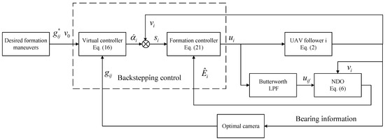
Figure 1.
The schematic diagram of the proposed bearing-only formation control strategy.
3.2. Stability Analysis
In Section 3.1, we can observe that the estimation error of the disturbance observer (6) remains bounded at all times. Thus, , where is a positive constant representing the maximum value of the estimation error of the nonlinear disturbance observer. Therefore, it is reasonable to transform the original problem 1 into designing a formation tracking control law ensuring that the formation tracking error and can converge to a small neighborhood of zero.
The main result is given as follows:
Theorem 1.
Under Assumption A1, Assumption A2 and Assumption A3 (see Appendix A for details), we consider a group of UAVs with the system dynamics given by Equation (2). The bearing-only formation control inputs are determined using Equation (21), with virtual control defined by Equation (16), and the nonlinear disturbance observer is given by Equation (6). With these conditions, problem 1 can be successfully addressed, demonstrating that the formation tracking error and can converge to a small neighborhood of zero.
Proof of Theorem 1.
By substituting the control law (21) into Equation (20), we obtain
where .
By applying Young’s inequality, we can establish the following inequality:
Substituting Equation (24) into Equation (23), we obtain
where .
By solving the above inequality, we obtain
where .
Based on the inequality (26), it can be determined that the Lyapunov function is bounded by . This implies that all signals of the control systems are uniformly ultimately bounded (UUB). It is worth noting that by increasing , the upper bound can be decreased. This means that formation tracking error and can be compelled to converge to a compact set around zero. Consequently, the proof of Theorem 1 is completed. □
4. Simulation Examples
In the simulation experiments, we conducted three distinct cases to evaluate the performance of the proposed controller. The first case aimed to verify the effectiveness of the controller in scenarios involving static formation control, constant velocity formation tracking control, and time-varying velocity formation tracking control. By examining these different control scenarios, we assessed the controller’s ability to achieve accurate and stable control under various conditions. The second case focused on testing the robustness of the controller. External perturbations and parameter perturbations were introduced to the control system to assess its ability to withstand disturbances and uncertainties. This case allowed us to evaluate the controller’s resilience and its capability to maintain control performance in the presence of external disturbances and parameter variations. The third case in this study aimed to validate the superiority of the proposed control method by comparing it with a traditional PD bearing-only formation method.
The formation shape depicted in Figure 2a represents a cube, comprising two leaders (highlighted in red) and six followers (highlighted in blue). The corresponding topology structure is illustrated in Figure 2b. The relative desired bearing values for the target formation are as follows: , , , , and other relative bearing information can be obtained using .
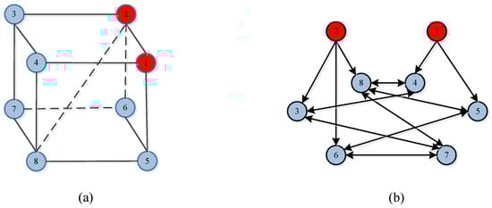
Figure 2.
The desired formation structure (a) and topology structure (b) for case 1 and case 2.
The formation shape depicted in Figure 3a represents a pentagon, consisting of two leaders (highlighted in red) and four followers (highlighted in blue). The corresponding topology structure is illustrated in Figure 3b. The relative desired bearing values for the target formation are as follows: , , , , , and other relative bearing information can be obtained using .
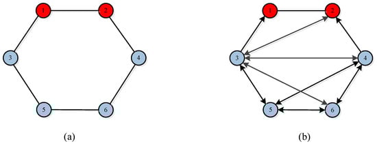
Figure 3.
The desired formation structure (a) and topology structure (b) for case 3.
4.1. Case 1: Bearing-Only Formation Control for UAVs
In this subsection, we conduct simulation experiments to evaluate the performance of the proposed formation tracking control strategies for UAVs. The experiments were carried out in three scenarios: static formation tracking, constant velocity formation tracking, and time-varying velocity formation tracking. The system model of UAVs is depicted as follows:
where
and , indicating the absence of external disturbances in the control systems. The control parameters are selected as , , , , , .
In the static formation simulation, the initial position and the velocity of the leaders are , , , respectively. The initial positions of the followers , , , , , , while their velocities are set to zero. The simulation results are shown in Figure 4.
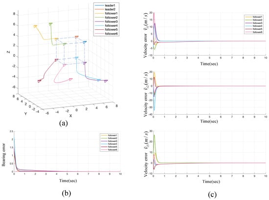
Figure 4.
Trajectories (a), bearing error (b), and velocity error (c) of the proposed formation control method for static formation case. The bearing error .
In the constant velocity formation tracking simulation, the initial position and the velocity of the leaders are , , , respectively. The initial positions of the followers are randomly selected, while their velocities are set to zero. The simulation results are shown in Figure 5.
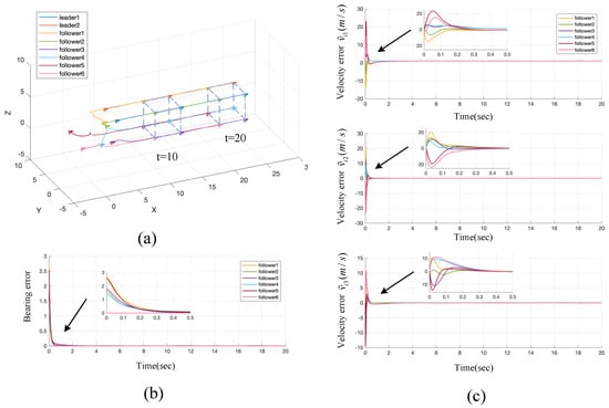
Figure 5.
Trajectories (a), bearing error (b), and velocity error (c) of the proposed formation control method for the constant velocity formation case. The bearing error .
In the time-varying velocity formation tracking simulation, the initial position and the velocity of the leaders are , , , respectively. The initial positions of the followers are randomly selected, while their velocities are set to zero. The simulation results are shown in Figure 6.
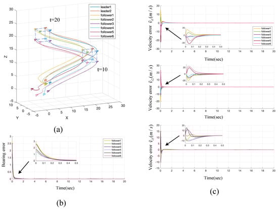
Figure 6.
Trajectories (a), bearing error (b), and velocity error (c) of the proposed formation control method for the time-varying velocity formation case. The bearing error .
Based on the simulation results, it can be concluded that the proposed approach successfully accomplishes the static formation, constant velocity tracking formation, and time-varying formation control missions. The bearing errors and velocity estimation errors exhibit convergence to zero, indicating the effectiveness of the approach.
4.2. Case 2: Bearing-Only Formation Control with Uncertainties and Disturbance
In this subsection, simulation experiments were conducted to assess the validity of the proposed bearing-only formation control approach in handling uncertainties and disturbances. The equations describing the UAV system are presented in Equation (2), with the distinction that the system incorporates parametric perturbations and external disturbances. The desired bearing and controller parameters remain unchanged from Section 4.1.
In the formation simulation with external disturbance, the initial position and the velocity of the leaders are , , , respectively. The initial positions of the followers are randomly selected, while their velocities are set to zero. At the 10th second of the simulation, an external disturbance, denoted as
impacts the system. The simulation results are shown in Figure 7a,c.
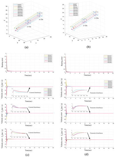
Figure 7.
Trajectories, bearing error, and velocity error of the proposed formation control method with uncertainties and disturbance. (a,c) The tracking formation case with external disturbance. (b,d) The tracking formation case with parameters disturbance. The bearing error .
In this simulation, the system is not subjected to external perturbations. Instead, it experiences parameter perturbations, as follows:
The simulation results are shown in Figure 7b,d.
Based on the simulation results, it can be observed that the control system exhibits slight jitter in the velocity tracking error and bearing error when subjected to uncertainties and external disturbances. However, the system quickly converges to zero, indicating that the proposed method in this paper effectively handles system uncertainties and disturbances with robustness.
4.3. Case 3: Comparison Simulation
In this subsection, the superiority of the controller proposed in this paper is verified via comparative simulations, mainly by comparing the control performance indexes of the control system. By conducting simulation experiments, the performance differences between the proposed controller and other methods can be evaluated and compared. These performance metrics include the stability, convergence speed, and robustness of the system. In the cited literature [22], the leader–follower formation strategy is employed, and a PD controller utilizing bearing information is devised for the double integral model to accomplish the objective of tracking the desired formation. As stated in the same literature [22], the control input for each follower is given in
where and are control parameters.
Given that the PD controller was specifically developed to address the formation tracking issue associated with the double integral model, it is not capable of handling the complex and nonlinear UAV formation tracking problem. Consequently, the system model of UAVs is represented as follows:
where , indicating the absence of external disturbances in the control systems and . It is important to note that the model in (31) does not incorporate the unknown nonlinear functions f1 and b of the system. It solely takes into account the external perturbation d for the purpose of comparing the system’s resilience. Furthermore, the model is limited to a second-order system, focusing exclusively on the motion in the x–y-axes and neglecting the vertical motion in the z-axis.
The desired formation structure and topology structure are shown in Figure 3. The control parameters for the proposed controller are , , , , , . The controller parameters for the PD control method are and . The initial position and the velocity of the leaders are , , , respectively. The initial positions of the followers are , , , and , while their velocities are set to zero. At the 10th second of the simulation, an external disturbance, denoted as
impacts the systems.
The comparative simulation results are shown in Figure 8, and a comparison of the control performance index parameters is given in Table 2. Before delving into the analysis of the results, it is essential to clarify that the convergence time (CT) is defined as the duration needed for the error to diminish to a value below 0.01.
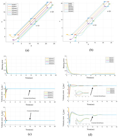
Figure 8.
Trajectories, bearing error, and velocity error of comparative simulation. (a,c) The proposed controller in this article. (b,d) The PD controller. The bearing error .
Table 2.
Comparison of control performance indicators.
Based on the simulation results, it is evident that both control approaches can successfully accomplish the formation tracking objective. However, when subjected to an external disturbance at the 10th second, the PD control system exhibits oscillations, while the controller proposed in this paper effectively rectifies the situation by applying a more suitable control input within a shorter duration, thereby rapidly converging towards the equilibrium point. Table 2 clearly demonstrates that the controller proposed in this paper outperforms the PD controller in terms of mean square error and convergence speed. Moreover, the proposed controller exhibits faster convergence even when subjected to perturbations, showcasing its robustness and superior performance.
5. Conclusions
This article presents a study on nonlinear disturbance observer-based bearing-only formation tracking control for UAV systems. The distributed control strategy utilized in the research relies on relative bearing information from neighboring UAVs. The article addresses the challenges posed by uncertainties and disturbances by introducing a novel nonlinear disturbance observer, which effectively mitigates their impact. Additionally, the problem of an unknown controller orientation is resolved through the implementation of a Butterworth low-pass filter. The proposed approach employs a backstepping control method to develop a bearing-only formation tracking controller. The stability of the closed-loop control systems is rigorously proven using Lyapunov theory. Numerical simulations are conducted to validate the effectiveness of the proposed scheme in achieving the objectives of formation control. Overall, this research contributes to the advancement of UAV systems by providing a robust control strategy for formation tracking in the presence of uncertainties and disturbances.
Author Contributions
Conceptualization, writing—original draft preparation, simulation results, and theoretical contribution, C.D.; supervision, project administration, and funding acquisition, J.Z.; writing—review and editing, C.D. and Z.Z. All authors have read and agreed to the published version of the manuscript.
Funding
This study was supported by China Postdoctoral Science Special Foundation (Grant Number: 2021TQ0102), National Natural Science Foundation of China (Grant Number: 62203158, Changsha Natural Science Foundation (Grant Number: kq2202175) and National Natural Science Foundation of Hunan Province (Grant Number: 2023JJ40182).
Data Availability Statement
Not applicable.
Conflicts of Interest
The authors declare no conflict of interest.
Appendix A
Assumption A1.
Graph G is assumed to be connected, and the submatrix is assumed to be nonsingular.
Remark A1.
Assumption A1 plays a crucial role in addressing the bearing-based formation control problem, as it ensures that only unique formations can be achieved through control approaches. Only when the bearing-based formation is unique can the desired position and velocity of each follower be determined with certainty. Lemma 1 further establishes the requirement for the submatrix to be nonsingular.
Assumption A2 (Collision Avoidance).
Using the evolution of the formation, neighboring agents maintain a safe distance to avoid colliding with each other. This implies that for all pairs of agents and for all time , the positions of the agents satisfy the condition , and the Euclidean distance between the positions of agents i and j, denoted as , is greater than or equal to a positive constant , which represents the minimum safe distance.
Remark A2.
Assumption A2, which is commonly adopted in existing formation control studies [15], reflects the importance of collision avoidance. Those who are interested in delving into this topic can refer to the literature [34] for further exploration.
Assumption A3.
The first and second leaders of the multi-agent systems naturally follow the desired tracking trajectory without any control input, meaning that their positions , where and are the desired position of the leaders, and their velocities and are equal to the desired velocity .
References
- Wu, Y.; Gou, J.; Hu, X.; Huang, Y. A new consensus theory-based method for formation control and obstacle avoidance of UAVs. Aerosp. Sci. Technol. 2020, 107, 106332. [Google Scholar] [CrossRef]
- Dou, L.; Cai, S.; Zhang, X.; Su, X.; Zhang, R. Event-triggered-based adaptive dynamic programming for distributed formation control of mul-ti-UAV. J. Frankl. Inst. 2022, 359, 3671–3691. [Google Scholar] [CrossRef]
- Wei, L.; Chen, M.; Li, T. Dynamic event-triggered cooperative formation control for UAVs subject to time-varying disturbances. IET Control Theory Appl. 2020, 14, 2514–2525. [Google Scholar] [CrossRef]
- Wang, S.; Yan, X.; Ma, F.; Wu, P.; Liu, Y. A novel path following approach for autonomous ships based on fast marching method and deep reinforcement learning. Ocean Eng. 2022, 257, 111495. [Google Scholar] [CrossRef]
- Zhao, Z.; Cao, D.; Yang, J.; Wang, H. High-order sliding mode observer-based trajectory tracking control for a quadrotor UAV with uncertain dynamics. Nonlinear Dyn. 2020, 102, 2583–2596. [Google Scholar] [CrossRef]
- Cao, L.; Yao, D.; Li, H.; Meng, W.; Lu, R. Fuzzy-based dynamic event triggering formation control for nonstrict-feedback nonlinear MASs. Fuzzy Sets Syst. 2023, 452, 1–22. [Google Scholar] [CrossRef]
- Chen, G.; Yao, D.; Zhou, Q.; Li, H.; Lu, R. Distributed event-triggered formation control of USVs with prescribed performance. J. Syst. Sci. Complex. 2022, 35, 820–838. [Google Scholar] [CrossRef]
- Fu, M.; Wang, L. A fixed-time distributed formation control of marine surface vehicles with actuator input saturation and time-varying ocean currents. Ocean Eng. 2022, 251, 111067. [Google Scholar] [CrossRef]
- Zhi, Y.; Liu, L.; Guan, B.; Wang, B.; Cheng, Z.; Fan, H. Distributed robust adaptive formation control of fixed-wing UAVs with unknown uncertainties and disturbances. Aerosp. Sci. Technol. 2022, 126, 107600. [Google Scholar] [CrossRef]
- Ziquan, Y.; Zhang, Y.; Jiang, B.; Jun, F.; Ying, J. A review on fault-tolerant cooperative control of multiple unmanned aerial vehicles. Chin. J. Aeronaut. 2022, 35, 1–18. [Google Scholar]
- Xu, Z.; Yan, T.; Yang, S.X.; Gadsden, S.A. Distributed Leader Follower Formation Control of Mobile Robots based on Bioinspired Neural Dynamics and Adaptive Sliding Innovation Filter. IEEE Trans. Ind. Inform. 2023; in press. [Google Scholar] [CrossRef]
- Wei, H.; Shen, C.; Shi, Y. Distributed Lyapunov-based model predictive formation tracking control for autonomous underwater vehicles subject to disturbances. IEEE Trans. Syst. Man Cybern. Syst. 2019, 51, 5198–5208. [Google Scholar] [CrossRef]
- He, S.; Xu, R.; Zhao, Z.; Zou, T. Vision-based neural formation tracking control of multiple autonomous vehicles with visibility and performance constraints. Neurocomputing 2022, 492, 651–663. [Google Scholar] [CrossRef]
- Van Tran, Q.; Kim, J. Bearing-constrained formation tracking control of nonholonomic agents without inter-agent communication. IEEE Control Syst. Lett. 2022, 6, 2401–2406. [Google Scholar] [CrossRef]
- Su, H.; Zhu, S.; Yang, Z.; Chen, C.; Guan, X. Bearing-based formation tracking control of AUVs with optimal gains tuning. Ocean Eng. 2022, 258, 111672. [Google Scholar] [CrossRef]
- Chen, L.; Sun, Z. Gradient-based bearing-only formation control: An elevation angle approach. Automatica 2022, 141, 110310. [Google Scholar] [CrossRef]
- Luo, X.; Li, X.; Li, X.; Guan, X. Bearing-only formation control of multi-agent systems in local reference frames. Int. J. Control 2021, 94, 1261–1272. [Google Scholar] [CrossRef]
- Wu, K.; Hu, J.; Lennox, B.; Arvin, F. Finite-time bearing-only formation tracking of heterogeneous mobile robots with collision avoidance. IEEE Trans. Circuits Syst. II Express Briefs 2021, 68, 3316–3320. [Google Scholar] [CrossRef]
- Zhao, J.; Yu, X.; Li, X.; Wang, H. Bearing-only formation tracking control of multi-agent systems with local reference frames and con-stant-velocity leaders. IEEE Control Syst. Lett. 2020, 5, 1–6. [Google Scholar] [CrossRef]
- Bae, Y.B.; Kwon, S.H.; Lim, Y.H.; Ahn, H.S. Distributed bearing-based formation control and network localization with exogenous disturbances. Int. J. Robust Nonlinear Control 2022, 32, 6556–6573. [Google Scholar] [CrossRef]
- Zhao, S.; Zelazo, D. Bearing rigidity and almost global bearing-only formation stabilization. IEEE Trans. Autom. Control 2015, 61, 1255–1268. [Google Scholar] [CrossRef]
- Zhao, S.; Li, Z.; Ding, Z. Bearing-only formation tracking control of multiagent systems. IEEE Trans. Autom. Control 2019, 64, 4541–4554. [Google Scholar] [CrossRef]
- Li, X.; Wen, C.; Fang, X.; Wang, J. Adaptive bearing-only formation tracking control for nonholonomic multiagent systems. IEEE Trans. Cybern. 2021, 52, 7552–7562. [Google Scholar] [CrossRef]
- Tang, Z.; Loría, A. Localization and tracking control of autonomous vehicles in time-varying bearing formation. IEEE Control Syst. Lett. 2022, 7, 1231–1236. [Google Scholar] [CrossRef]
- Su, H.; Chen, C.; Yang, Z.; Zhu, S.; Guan, X. Bearing-Based Formation Tracking Control with Time-Varying Velocity Estimation. IEEE Control Syst. Lett. 2022; in press. [Google Scholar] [CrossRef]
- Amirkhani, A.; Barshooi, A.H. Consensus in multi-agent systems: A review. Artif. Intell. Rev. 2022, 55, 3897–3935. [Google Scholar] [CrossRef]
- Bao, G.; Ma, L.; Yi, X. Recent advances on cooperative control of heterogeneous multi-agent systems subject to constraints: A survey. Syst. Sci. Control Eng. 2022, 10, 539–551. [Google Scholar] [CrossRef]
- Li, Z.; Tnunay, H.; Zhao, S.; Meng, W.; Xie, S.Q.; Ding, Z. Bearing-only formation control with prespecified convergence time. IEEE Trans. Cybern. 2020, 52, 4620–4629. [Google Scholar] [CrossRef]
- Zhao, J.; Li, X.; Yu, X.; Wang, H. Finite-time cooperative control for bearing-defined leader-following formation of multiple dou-ble-integrators. IEEE Trans. Cybern. 2021, 52, 13363–13372. [Google Scholar] [CrossRef]
- Zhao, S.; Zelazo, D. Localizability and distributed protocols for bearing-based network localization in arbitrary dimensions. Automatica 2016, 69, 334–341. [Google Scholar] [CrossRef]
- Dong, X.; Yu, B.; Shi, Z.; Zhong, Y. Time-varying formation control for unmanned aerial vehicles: Theories and applications. IEEE Trans. Control Syst. Technol. 2014, 23, 340–348. [Google Scholar] [CrossRef]
- Bu, X.; Wu, X.; Zhang, R.; Ma, Z.; Huang, J. Tracking differentiator design for the robust backstepping control of a flexible air-breathing hy-personic vehicle. J. Frankl. Inst. 2015, 352, 1739–1765. [Google Scholar] [CrossRef]
- Li, X.; Wen, C.; Chen, C. Adaptive formation control of networked robotic systems with bearing-only measurements. IEEE Trans. Cybern. 2020, 51, 199–209. [Google Scholar] [CrossRef]
- Mondal, A.; Bhowmick, C.; Behera, L.; Jamshidi, M. Trajectory tracking by multiple agents in for-mation with collision avoidance and connectivity assurance. IEEE Syst. J. 2017, 12, 2449–2460. [Google Scholar] [CrossRef]


Disclaimer/Publisher’s Note: The statements, opinions and data contained in all publications are solely those of the individual author(s) and contributor(s) and not of MDPI and/or the editor(s). MDPI and/or the editor(s) disclaim responsibility for any injury to people or property resulting from any ideas, methods, instructions or products referred to in the content. |
© 2023 by the authors. Licensee MDPI, Basel, Switzerland. This article is an open access article distributed under the terms and conditions of the Creative Commons Attribution (CC BY) license (https://creativecommons.org/licenses/by/4.0/).