Stability and Hopf Bifurcation Analysis for a Phage Therapy Model with and without Time Delay

Abstract

This study proposes a mathematical model that accounts for the interaction of bacteria, phages, and the innate immune response with a discrete time delay. First, for the non-delayed model we determine the local and global stability of various equilibria and the existence of Hopf bifurcation at the positive equilibrium. Second, for the delayed model we provide sufficient conditions for the local stability of the positive equilibrium by selecting the discrete time delay as a bifurcation parameter; Hopf bifurcation happens when the time delay crosses a critical threshold. Third, based on the normal form method and center manifold theory, we derive precise expressions for determining the direction of Hopf bifurcation and the stability of bifurcating periodic solutions. Finally, numerical simulations are performed to verify our theoretical analysis.

1. Introduction

Phages are viruses that infect prokaryotic organisms, and are important components of ecological systems [1]. Phages infect bacteria by injecting their genetic material into cells. When the virus enters the cell, it prevents other phages from attacking it and begins to reproduce within the host until the number of new viral particles reaches the bacterial threshold [2,3]. The use of bacteriophages to treat bacterial infections, commonly referred to as phage therapy, dates back to the early 20th century. Phage treatment can be more effective than antibiotics in treating various medical conditions [4]. Moreover, phage therapy has multiple potential applications, and can even be employed in place of antibiotics in certain circumstances [5]. Clinical research on phage therapy has not shown any of the severe side effects such as anaphylaxis that are sometimes associated with antibiotics [6].

Mathematical models are widely used in various fields, including biology, epidemiology, engineering, physics, sciences, business, and computer science. They help us to understand ecosystem dynamics, quantify disease control strategies, and gain new theoretical insights into nature [7]. Nonlinear dynamical systems are commonly used to describe biological systems and relationships between individuals. Researchers have developed nonlinear dynamical systems for various biological phenomena, including stability, persistence, and bifurcation. Mathematical modeling of phage therapy is crucial for understanding bacteria–bacteriophage interactions and their long-term behavior. Various models have been constructed, resulting in numerous beneficial outcomes [2,8,9,10,11,12,13,14,15,16].

Considering that the evolution of a system is dependent on its present and previous states, time delays must be included in the model. Accordingly, authors have focused on dynamic behaviors such as stability and the existence of Hopf bifurcations in delayed population models [17,18,19,20]. The above-mentioned references have investigated the existence and direction of Hopf bifurcations and the stability of positive equilibria. The application of delay differential equations to the modeling of biological phenomena has gained popularity in recent years. In particular, several studies have presented bacteria–bacteriophage models by introducing a time delay to generate more realistic models; see for example [21,22,23,24,25,26] and references therein. Meanwhile, due to the complexity of the impacts of delay on a system’s dynamic behavior, researchers have increasingly focused on the dynamic behavior of delayed phage therapy models, such as their stability and the occurrence of Hopf bifurcations. In a model of a delayed marine bacteriophage infection, Beretta et al. [21] analysed the global and local stability of the equilibrium. Beretta and Solimano [22] expanded upon their previous research [21] to investigate how delay impacts equilibrium stability. In [23], the author addressed models of marine phage infection with delay and stage structure achieving the persistence and extinction of the system under specific conditions. Gakkhar and Sahani [24] proposed a model of bacteria–bacteriophage interaction with a constant delay. They examined a simple Hopf bifurcation for the non-zero equilibrium point and outlined the conditions for a susceptible bacteria-free equilibrium and its stability. Casino et al. [27] identified the optimal lysis time for bacteria–phage interactions in a structured cell population model. Additional delayed bacteria–phage models can be found in [28,29,30,31] and the references cited therein. Several significant studies have been published on diffusion-based bacteriophage models [32,33,34]. Mathematically rigorous studies of stochastic models for bacteriophage infection with and without time delay have been published as well [35,36,37,38,39].

Understanding the interactions between bacteria, phages, and the immune system is essential to developing successful bacteriophage therapeutics. Meanwhile, bacteriophage-based bacterial elimination has therapeutic potential and is currently utilized to treat bacterial infections [40,41]. Mathematical models of bacteria–phage interactions that include immune responses are of growing interest to the authors. Leung and Weitz [42] proposed a nonlinear ODE phage therapy model involving bacterial, phage, and immune system interactions:

$$\left\{\begin{array}{cc}\hfill \dot{B}& =rB\left(1-\frac{B}{K_C}\right)-\varphi BP-\frac{ϵIB}{1+B/K_D},\hfill \\ \hfill \dot{P}& =\beta \varphi BP-wP,\hfill \\ \hfill \dot{I}& =\alpha I\left(1-\frac{I}{K_I}\right)\frac{B}{B+K_N},\hfill \end{array}\right.$$

(1)

where $B\left(t\right)$, $P\left(t\right)$, and $I\left(t\right)$ represent the concentrations of bacteria, phages, and the immune system at time t, respectively, and r and $K_C$ represent the maximum growth rate and carrying capacity of the bacteria, respectively. The phages attach to and infect the bacteria with an adsorption rate of $\varphi$ and release new virus particles with a burst size of $\beta$. The phage particles decay with the death rate w. The presence of bacteria with a maximum growth rate $\alpha$ activates the immune system. Meanwhile, the immune carrying capacity is $K_I$ and the killing parameter is $ϵ$. Finally, $K_D$ is the bacterial density when the host immune response is half-saturated and $K_N$ is the bacterial concentration at which the innate immunity growth rate is at half its maximum.

In [42], Leung and Weitz simplified the above System (1) by employing a quasistatic approximation in which the innate immune response is represented as a constant. This simplification is reasonable considering that the concentrations of bacteria and phages are expected to change more rapidly than the immune response. They applied this approximation when the innate immune response reached its maximum $K_I$. This resembles a circumstance in which the innate immune response does not control bacterial infection. Phages are then included as an additional treatment. In this case, the model equation in (1) reduces to

$$\left\{\begin{array}{cc}\hfill \dot{B}& =rB\left(1-\frac{B}{K_C}\right)-\varphi BP-\frac{ϵK_{I}B}{1+B/K_D},\hfill \\ \hfill \dot{P}& =\beta \varphi BP-wP,\hfill \end{array}\right.$$

(2)

with the initial conditions

$$B\left(0\right)\ge 0,P\left(0\right)\ge 0.$$

In [42], Leung and Weitz discovered a synergistic regime in which the phage and immune system cooperate to eradicate bacteria. They demonstrated that the interaction between phages and the immune system is essential in order for phage therapy to effectively eliminate bacterial infections. However, they did not discuss the dynamic behaviors of (1) and (2), such as positivity, boundedness, persistence, stability, Hopf bifurcation analysis, etc. In [43], we examined the mathematical dynamics analysis of the model in (1) formulated by Leung and Weitz [42], studied the persistence, non-persistence, and local stability of possible equilibrium solutions, and provided the criteria for the global stability of the planar and positive equilibria. However, the analysis of such dynamics for the model in (2) was not completed in our previous paper [43].

Determining how delays influence the system’s stability, dynamics, and bifurcation is a challenging mathematical problem, and nonlinear dynamical bacteria–bacteriophage systems with time delays are extremely challenging because of the application of nonlinear biological phenomena and their dynamic behavior. There are a number of papers in the literature on modeling bacteria–bacteriophage systems using delay differential equations. Inspired by this previous literature, it appears that the model can be made more realistic by incorporating additional terms such as the time delay obtained from the past states of the system. For example, as noted in [21], the introduction of time delay can induce the system to exhibit complex dynamic behaviors, a development that is vital for advancing phage therapy. As far as we know, this model (2) has yet to be studied with the incorporation of a time delay and analysis of its dynamic behavior, making the present study an important one.

Motivated by the above discussion and based on [33], in this paper we assume that the recruitment of phages and the infection of bacteria both require discrete time lags and introduce a discrete time delay into System (2). Such a model is more biologically realistic than existing models. Based on the work of [42], the delay-induced modified model is represented by

$$\left\{\begin{array}{cc}\hfill \dot{B}& =rB\left(1-\frac{B}{K_C}\right)-\varphi BP-\frac{ϵK_{I}B}{1+B/K_D},\hfill \\ \hfill \dot{P}& =\beta \varphi B(t-\tau )P(t-\tau )-wP.\hfill \end{array}\right.$$

(3)

subject to the initial conditions $B_0\left(\nu \right)={\chi }_1\left(\nu \right)>0$, $P_0\left(\nu \right)={\chi }_2\left(\nu \right)>0$ and $\nu \in [-\tau ,0]$, where ${\chi }_{\gamma }\in C([-\tau ,0]⟶{\mathbb{R}}_{+})$ and $(\gamma =1,2)$ are given functions and $\tau$ is a positive constant.

According to other related studies, for example, [21,26,28,33], etc., the delay can destabilize the coexistence equilibrium and lead to the Hopf bifurcation of the system. Therefore, in this paper there is a real need to pose the important question of whether the delay causes System (3) to display these characteristics. Motivated by this fact, we introduce System (3) by adding a time delay term to System (2), then study the effects of delay on the dynamics of the system.

The remaining sections of this paper are organized as follows: in Section 2, we examine results relating to the non-delayed model, including the local and global stability of the positive equilibrium and the occurrence of Hopf bifurcation; Section 3 discusses similar results along with the stability and the direction of Hopf bifurcation for the delayed model; in Section 4, we conduct numerical simulations to verify our analytical results; finally, Section 5 presents the conclusions of this study.

2. Dynamics of the Non-Delayed Model

2.1. Positivity and Boundedness

In this context, positivity indicates that the population survives and boundedness represents a natural growth restriction due to limited resources. This subsection analyses the positivity and boundedness of the model in (2). In theoretical ecology, the biologically well-behaved nature of a system is established through its positivity and boundedness. Thus, System (2) has the following outcome.

Lemma 1.

System (2) has solutions $\left(B\right(t),P(t\left)\right)$ in the interval $\left[0,\infty \right)$ that satisfy $B\left(t\right)\ge 0$, $P\left(t\right)\ge 0$, and $\forall t\ge 0$.

Proof. 

The model in (2) can be written in matrix form:

$$\begin{array}{cc}\hfill \dot{X}& =\mathcal{G}\left(X\right),\hfill \\ \hfill X& ={(x_1,x_2)}^T={(B,P)}^T\in {\mathbb{R}}^2\hfill \end{array}$$

where $\mathcal{G}\left(X\right)$ is provided by

$$\mathcal{G}\left(X\right)=\left(\begin{array}{c}{\mathcal{G}}_1\left(X\right)\\ {\mathcal{G}}_2\left(X\right)\end{array}\right)=\left(\begin{array}{c}rB\left(1-\frac{B}{K_C}\right)-\varphi BP-\frac{ϵK_{I}B}{1+B/K_D}\\ \beta \varphi BP-wP\end{array}\right).$$

Because $\mathcal{G}\left(X\right)$ and $\frac{\partial \mathcal{G}}{\partial X}$ are continuous in ${\mathbb{R}}_{+}^2$, it is the case that $\mathcal{G}:{\mathbb{R}}_{+}^2\to {\mathbb{R}}^2$ is locally Lipschitz. By the standard theory of the ODE system, it follows that model (2) has a unique solution for any initial condition $X\left(0\right)=X_0=(B\left(0\right),P\left(0\right))\in {\mathbb{R}}_{+}^2$.

Further, the model in (2) can be rewritten as

$$\frac{dB}{dt}=B{\varphi }_1(B,P),\frac{dP}{dt}=P{\varphi }_2(B,P),$$

where

$$\begin{array}{cc}\hfill {\varphi }_1(B,P)& =r-\frac{r}{K_C}B-\varphi P-\frac{ϵK_I}{1+B/K_D},\hfill \\ \hfill {\varphi }_2(B,P)& =\beta \varphi B-w.\hfill \end{array}$$

$$\therefore \frac{dB}{dt}=B{\varphi }_1(B,P)\Rightarrow \frac{1}{B}dB={\varphi }_1(B,P)$$

By integrating, we obtain

$$\begin{array}{cc}\hfill \ln B& =\int {\varphi }_1(B,P)dt+\ln C\hfill \\ \hfill \Rightarrow B& =\exp [\int {\varphi }_1(B,P)dt+\ln C]=C\exp [\int {\varphi }_1(B,P)dt].\hfill \end{array}$$

It follows that

$$B\left(t\right)=B\left(0\right)\exp \left[{\int }_0^t{\varphi }_1(B\left(s\right),P\left(s\right))ds\right],$$

where $C=B\left(0\right)$. Thus, $B\left(t\right)$ is always positive, as $B\left(0\right)>0$. Similarly, from second equation of System (2) we can find the positivity of $P\left(t\right)$, as $P\left(0\right)>0$. Hence,

$$\begin{array}{cc}\hfill B\left(t\right)& =B\left(0\right)\exp \left[{\int }_0^t{\varphi }_1(B\left(s\right),P\left(s\right))ds\right]\ge 0,\hfill \\ \hfill P\left(t\right)& =P\left(0\right)\exp \left[{\int }_0^t{\varphi }_2(B\left(s\right),P\left(s\right))ds\right]\ge 0.\hfill \end{array}$$

Thus, the solution $X\left(t\right)=\left(B\right(t),P(t\left)\right)$ with initial condition $X\left(0\right)=X_0=(B\left(0\right),P\left(0\right))\in {\mathbb{R}}_{+}^2$ remains positive throughout the region ${\mathbb{R}}_{+}^2$. □

We next investigate whether the model in (2) is bounded within a particular region of the dynamical space.

To demonstrate the uniform boundedness of the model in (2), the following comparison lemma [44,45] is needed.

Lemma 2

(Comparison lemma). If $K\left(t\right)$ is an absolutely continuous function which satisfies the differential inequality

$$\frac{d\left(K\right(t\left)\right)}{dt}+{\sigma }_{1}K\left(t\right)\le {\sigma }_2,such thatt\ge 0,$$

where $({\sigma }_1,{\sigma }_2)\in {\mathbb{R}}^2$ and ${\sigma }_1\ne 0$, then for all $t\ge \widehat{T}\ge 0$ we have

$$K\left(t\right)\le \frac{{\sigma }_2}{{\sigma }_1}-\left(\frac{{\sigma }_2}{{\sigma }_1}-K\left(\widehat{T}\right)\right){\mathrm{e}}^{-{\sigma }_1(t-\widehat{T})}.$$

Remark 1.

All solutions of System (2) initiating in ${\mathbb{R}}_{+}^2$ are subject to the region $G=\{(B,P)\in {\mathbb{R}}_{+}^2:\varpi \left(t\right)\le \frac{\upsilon }{w}\}$ with $\upsilon :=\beta \frac{K_C}{4r}{(r+w)}^2$, as $t\to \infty$ for all positive initial values $(B\left(0\right),P\left(0\right))\in {\mathbb{R}}_{+}^2$, where $\varpi \left(t\right)=\beta B\left(t\right)+P\left(t\right)$. Using Comparison Lemma 2, we establish the outcome for a delay system. The proof follows in a similar fashion; see Theorem 6 as well.

2.2. Existence of Equilibrium Points

This subsection demonstrates that the model in (2) has different equilibrium solutions. The following are the probable equilibria of System (2) according to [43] and simple calculation:

1. Trivial equilibrium: $E_0=(0,0)$

2. Boundary equilibrium (phage-free equilibrium): $E_1=(\overline{B},0)$, where

$\overline{B}=\frac{K_C-K_D}{2}+\sqrt{\frac{{(K_C+K_D)}^2}{4}-\frac{ϵK_I{K}_C{K}_D}{r}}$ with $K_C>K_D$ and $r>ϵK_I$

3. Interior equilibrium: $E_2=(B^{\ast },P^{\ast })$, where

$$B^{\ast }=\frac{w}{\beta \varphi },P^{\ast }=\frac{1}{\varphi }\left(r(1-\frac{w}{\beta \varphi K_C})-\frac{ϵK_I}{1+w/\beta \varphi K_D}\right)$$

(4)

with

$$r>\frac{ϵ{\beta }^2{\varphi }^2{K}_I{K}_C{K}_D}{(\beta \varphi K_C-w)(w+\beta \varphi K_D)}\mathrm{and}w<\beta \varphi K_C$$

(5)

2.3. Stability Analysis

Stability refers to a system’s ability to resist small perturbations. Stability analysis is an acceptable tool for studying the long-term behavior of dynamic systems. In this subsection, we discuss the local and global stability and bifurcation analysis of System (2).

2.3.1. Stability Analysis of $E_0=(0,0)$

Theorem 1.

(i) 

The equilibrium $E_0=(0,0)$ is locally asymptotically stable if $r<ϵK_I$.

(ii) 

If the parameter r reaches the transcritical threshold $r=r_{tc}=ϵK_I$, a transcritical bifurcation arises around $E_0$ for System (2).

Proof. 

To acquire the local stability outcomes, we employ the Jacobian matrix related to System (2):

$$J(B,P)=\left(\begin{array}{cc}r-\frac{2r}{K_C}B-\varphi P-\frac{ϵK_I}{{(1+B/K_D)}^2}& -\varphi B\\ \beta \varphi P& \beta \varphi B-w\end{array}\right).$$

(i) The Jacobian matrix of System (2) at $E_0$ is

$$J\left(E_0\right)=\left(\begin{array}{cc}r-ϵK_I& 0\\ 0& -w\end{array}\right).$$

Thus, the trace and determinant of the matrix $J\left(E_0\right)$ are $\mathrm{tr}\left(J\left(E_0\right)\right)=r-ϵK_I-w$ and $\det \left(J\left(E_0\right)\right)=-w(r-ϵK_I)$, respectively. If $r<ϵK_I$, then $\mathrm{tr}\left(J_{\ast }\left(E_0\right)\right)<0$ and $\det \left(J\left(E_0\right)\right)>0$, and $E_0$ is locally asymptotically stable. Hence, $E_0$ is always unstable (saddle) when $r>ϵK_I$.

(ii) To demonstrate Theorem 1 (ii), we can use the transversality criteria based on Sotomayor’s theorem [46]. To use Sotomayor’s theorem, one of the eigenvalues of the matrix $J\left(E_0\right)$ must be zero at the bifurcation point $r_{tc}$. One eigenvalue of $J\left(E_0\right)$ disappears at $r=r_{tc}=ϵK_I$, while the other is $-w<0$. Let $\Delta ={({\delta }_1,{\delta }_2)}^T$ and ${\rm Y}={({\gamma }_1,{\gamma }_2)}^T$ represent the eigenvectors of $J\left(E_0\right)$ and $J^T\left(E_0\right)$ with zero eigenvalue, respectively. Then, $\Delta ={\rm Y}={[1,0]}^T$.

We define $S(B,P)={\left[V(B,P),W(B,P)\right]}^T$.

Therefore,

$$S_r(B,P)={\left[\frac{\partial V(B,P)}{\partial r},\frac{\partial W(B,P)}{\partial r}\right]}^T={\left[B(1-B/K_C),0\right]}^T,$$

which provides

$${{\rm Y}}^T\left[S_r(B,P)\right]=[1,0]{\left[B(1-B/K_C),0\right]}^T=B(1-B/K_C).$$

Hence, we have ${{\rm Y}}^T\left[S_r\left(E_0;r_{tc}\right)\right]=0$.

Now,

$$D{S}_r:=\left(\begin{array}{cc}\frac{\partial V_r}{\partial B}& \frac{\partial V_r}{\partial P}\\ \frac{\partial W_r}{\partial B}& \frac{\partial W_r}{\partial P}\end{array}\right)=\left(\begin{array}{cc}1-\frac{2B}{K_C}& 0\\ 0& 0\end{array}\right).$$

Thus, we have ${{\rm Y}}^T\left[D{S}_r\left(E_0;r_{tc}\right)\Delta \right]=[1,0]{[1,0]}^T=1\ne 0$, where

$$D{S}_r\left(E_0;r_{tc}\right)=\left(\begin{array}{cc}1& 0\\ 0& 0\end{array}\right).$$

Now, we can check the transversality condition.

Here,

$$D^{2}S(\Delta ,\Delta )=\left(\begin{array}{c}{V}_{BB}{\delta }_1{\delta }_1+V_{BP}{\delta }_1{\delta }_2+V_{PB}{\delta }_2{\delta }_1+V_{PP}{\delta }_2{\delta }_2\\ W_{BB}{\delta }_1{\delta }_1+W_{BP}{\delta }_1{\delta }_2+W_{PB}{\delta }_2{\delta }_1+W_{PP}{\delta }_2{\delta }_2\end{array}\right),$$

where $V_{BB}(0,0)=-\frac{2r}{K_C}+\frac{2ϵK_I}{K_D}$, $V_{BP}(0,0)=V_{PB}(0,0)=-\varphi <0$, $V_{PP}(0,0)=0$, $W_{BB}(0,0)=0$, $W_{BP}(0,0)=W_{PB}(0,0)=\beta \varphi >0$, and $W_{PP}(0,0)=0.$

Thus, $D^{2}S\left((0,0);r_{tc}\right)(\Delta ,\Delta )={\left[-\frac{2r}{K_C}+\frac{2ϵK_I}{K_D},0\right]}^T$, meaning that we have

$${{\rm Y}}^T\left[D^{2}S\left((0,0);r_{tc}\right)(\Delta ,\Delta )\right]=[1,0]{\left[-\frac{2r}{K_C}+\frac{2ϵK_I}{K_D},0\right]}^T=\left[-\frac{2r}{K_C}+\frac{2ϵK_I}{K_D}\right]\ne 0.$$

Hence, the system undergoes a supercritical transcritical bifurcation at $E_0$. The proof is now complete. □

Remark 2.

When $r<ϵK_I$, it is easy to observe that the trivial equilibrium $E_0$ is locally asymptotically stable and that the phage-free equilibrium $E_1$ does not exist. In contrast, the existence of $E_1$ implies the instability of $E_0$. Furthermore, the above discussion provides information regarding the experience of transcritical bifurcation around $E_0$.

2.3.2. Stability Analysis of $E_1=(\overline{B},0)$

Theorem 2.

(i) 

The phage-free equilibrium $E_1=(\overline{B},0)$ is locally asymptotically stable if

$$r<\frac{ϵK_I{K}_C{K}_D^2}{(K_C-2\overline{B}){(\overline{B}+K_D)}^2}andw>\beta \varphi \overline{B}.$$

(ii) 

The equilibrium $E_1=(\overline{B},0)$ is globally asymptotically stable in the interior of the first quadrant of the plane.

Proof. 

(i) The variational matrix of the equilibrium $E_1=(\overline{B},0)$ is

$$J\left(E_1\right)=\left(\begin{array}{cc}r-\frac{2r}{K_C}\overline{B}-\frac{ϵK_I{K}_D^2}{{(\overline{B}+K_D)}^2}& -\varphi \overline{B}\\ 0& \beta \varphi \overline{B}-w\end{array}\right).$$

The roots of $J\left(E_1\right)$ are $r-\frac{2r}{K_C}\overline{B}-\frac{ϵK_I{K}_D^2}{{(\overline{B}+K_D)}^2}$, $\beta \varphi \overline{B}-w$. Hence, $E_1$ is locally asymptotically stable if $r<\frac{ϵK_I{K}_C{K}_D^2}{(K_C-2\overline{B}){(\overline{B}+K_D)}^2}$ and $w>\beta \varphi \overline{B}$.

(ii) Let $(B,P)\in {\mathbb{R}}_{+}^2:\{(B,P)\in {\mathbb{R}}^2:B>0,P>0\}$ and consider the function $L^{\ast }:{\mathbb{R}}_B^2⟶\mathbb{R}$,

$$L^{\ast }(B,P)=b_1(B-\overline{B}-\overline{B}\ln (B/\overline{B})).$$

(6)

The derivative of (6) along the solutions of System (2) is

$$\frac{d{L}^{\ast }}{dt}=b_1\frac{1}{B}(B-\overline{B})\frac{dB}{dt}=b_1(B-\overline{B})\left[r\left(1-\frac{B}{K_C}\right)-\frac{ϵK_I}{1+B/K_D}\right].$$

(7)

Because $E_2(B^{\ast },P^{\ast })$ satisfies (2), after a simple calculation we obtain

$$r\left(1-\frac{\overline{B}}{K_C}\right)=\frac{ϵK_I}{1+\overline{B}/K_D}.$$

(8)

Replacing (7) with (8), we obtain

$$\begin{array}{cc}\hfill \frac{d{L}^{\ast }}{dt}& =b_1(B-\overline{B})\left[r\left(1-\frac{B}{K_C}\right)-r\left(1-\frac{\overline{B}}{K_C}\right)\right]\hfill \\ & =b_1(B-\overline{B})\left[-\frac{r}{K_C}\left(B-\overline{B}\right)\right]\hfill \\ & =\frac{-r{b}_1}{K_C}{(B-\overline{B})}^2<0.\hfill \end{array}$$

According to the negative coefficients of the square terms, $\frac{d{L}^{\ast }}{dt}$ is less than zero along all trajectories in the plane except $E_2(B^{\ast },P^{\ast })$. Therefore, $E_2(B^{\ast },P^{\ast })$ is globally asymptotically stable. □

2.3.3. Stability and Hopf Bifurcation of $E_2=(B^{\ast },P^{\ast })$

Theorem 3.

Assume that $r^{\ast }=\frac{ϵ{\beta }^2{\varphi }^2{K}_I{K}_C{K}_D}{{(w+\beta \varphi K_D)}^2}$ and that (5) holds. The following assertions are obtained:

(i) The equilibrium $E_2$ of System (2) is locally asymptotically stable if $r>r^{\ast }$ and unstable if $r<r^{\ast }$.

(ii) If $r=r^{\ast }$, System (2) experiences Hopf bifurcation at $E_2$, and $r^{\ast }$ is the system’s critical value.

Proof. 

The Jacobian matrix of System (2) at the interior equilibrium $E_2=(B^{\ast },P^{\ast })$ is

$$J\left(E_2\right)=\left(\begin{array}{cc}r-\frac{2r}{K_C}{B}^{\ast }-\varphi P^{\ast }-\frac{ϵK_I}{{(1+B^{\ast }/K_D)}^2}& -\varphi B^{\ast }\\ \beta \varphi P^{\ast }& \beta \varphi B^{\ast }-w\end{array}\right).$$

Substituting the values of $B^{\ast }$ and $P^{\ast }$ described in (4) into $J\left(E_2\right)$, we obtain

$$J_{\ast }\left(E_2\right)=\left(\begin{array}{cc}\frac{ϵw\beta \varphi K_I{K}_D}{{(w+\beta \varphi K_D)}^2}-\frac{rw}{\beta \varphi K_C}& -\frac{w}{\beta }\\ \frac{r(\beta \varphi K_C-w)}{\varphi K_C}-\frac{ϵ{\beta }^2\varphi K_I{K}_D}{w+\beta \varphi K_D}& 0\end{array}\right).$$

The characteristic equation of $J_{\ast }\left(E_2\right)$ is

$${\lambda }^2-\mathrm{tr}\left(J_{\ast }\left(E_2\right)\right)\lambda +\det \left(J_{\ast }\left(E_2\right)\right)=0,$$

(9)

$$\begin{array}{cc}tr\left(J_{\ast }\left(E_2\right)\right)\hfill & =-\frac{rw}{\beta \varphi K_C}+\frac{ϵw\beta \varphi K_I{K}_D}{{(w+\beta \varphi K_D)}^2},\hfill \\ \det \left(J_{\ast }\left(E_2\right)\right)\hfill & =\frac{w}{\beta }\left[\frac{r(\beta \varphi K_C-w)}{\varphi K_C}-\frac{ϵ{\beta }^2\varphi K_I{K}_D}{w+\beta \varphi K_D}\right].\hfill \end{array}$$

(i) If $r>r^{\ast }=\frac{ϵ{\beta }^2{\varphi }^2{K}_I{K}_C{K}_D}{{(w+\beta \varphi K_D)}^2}$, then $\mathrm{tr}\left(J_{\ast }\left(E_2\right)\right)<0$, and the existence condition (5) of $E_2$ implies $\det \left(J_{\ast }\left(E_2\right)\right)>0$. Thus, the characteristic Equation (9) has negative real parts, as $\mathrm{tr}\left(J_{\ast }\left(E_2\right)\right)<0$ and $\det \left(J_{\ast }\left(E_2\right)\right)>0$. Hence, $E_2=(B^{\ast },P^{\ast })$ is locally asymptotically stable in B-P space for $r>r^{\ast }$. Moreover, $E_2$ is unstable in that space for $r<r^{\ast }$.

(ii) It is obvious that if $\mathrm{tr}\left(J_{\ast }\left(E_2\right)\right)=0$ and $\det \left(J_{\ast }\left(E_2\right)\right)>0$, then both of the roots must be purely imaginary. Thus, from the implicit function theorem a Hopf bifurcation emerges in which a periodic orbit is generated as the stability of the equilibrium point $E_2$ varies. The critical value of Hopf bifurcation parameter is defined by $r=r^{\ast }=\frac{ϵ{\beta }^2{\varphi }^2{K}_I{K}_C{K}_D}{{(w+\beta \varphi K_D)}^2}$. From the above analysis, it is easy to see that under the given conditions we have the following: (a) $\mathrm{tr}\left(J_{\ast }\left(E_2\right)\right)=0$, (b) $\det \left(J_{\ast }\left(E_2\right)\right)>0$, and (c) $\frac{d}{dr}\mathrm{tr}\left(J_{\ast }\left(E_2\right)\right)=-\frac{w}{\beta \varphi K_C}\ne 0$ at $r=r^{\ast }$. This result guarantees the presence of Hopf bifurcation around the positive equilibrium $E_2$. The proof is complete. □

2.3.4. Non-Existence of Non-Trivial Periodic Solution of System (2)

It is essential to determine whether an ecological system has a periodic solution, as the existence of such a solution can lead to complex ecological phenomena. On the one hand, the nonexistence of a periodic solution can convert a locally stable equilibrium into a globally stable one. In this subsection, using the Dulac–Bendixon criterion [46], we demonstrate the non-existence of periodic solutions to System (2).

Theorem 4.

If there exists a continuously differentiable function $\Theta (B,P)$ in the interior of ${\mathbb{R}}_{+}^n$ such that $\overrightarrow{\nabla }·(\Theta S)$ has constant sign and is not identically zero in any subregion, then system (2) does not possess any limit cycle, and in fact has a closed trajectory which lies entirely within ${\mathbb{R}}_{+}^n$.

Proof. 

Construct the Dulac function as $\Theta (B,P)=\frac{1}{BP}$ and a $C^1$ vector field defined in ${\mathbb{R}}_{+}^{20}$ as $S(B,P)=(V,W)=\left(rB-\frac{r}{K_C}{B}^2-\varphi BP-\frac{ϵK_{I}B}{1+B/K_D},\beta \varphi BP-wP\right)$. Clearly, $\Theta \in C^1\left({\mathbb{R}}_{+}^{20}\right)$, where ${\mathbb{R}}_{+}^{20}$ is the interior of ${\mathbb{R}}_{+}^n$. Moreover, it is clear that $\Theta (B,P)>0$ in ${\mathbb{R}}_{+}^{n0}$. We obtain

$$\begin{array}{cc}\hfill \overrightarrow{\nabla }·(\Theta S)& =\frac{\partial }{\partial B}(\Theta V)+\frac{\partial }{\partial P}(\Theta W)\hfill \\ \hfill & =\frac{1}{P}\frac{\partial }{\partial B}\left(r-\frac{r}{K_C}B-\varphi P-\frac{ϵK_I}{1+B/K_D}\right)+\frac{1}{B}\frac{\partial }{\partial P}\left(\beta \varphi B-w\right)\hfill \\ \hfill & =\frac{1}{P}\left(-\frac{r}{K_C}+\frac{ϵK_I{K}_D}{{(B+K_D)}^2}\right)\hfill \\ \hfill & <0,\mathrm{provided}r>\frac{ϵ{\beta }^2{\varphi }^2{K}_I{K}_C{K}_D}{{(w+\beta \varphi K_D)}^2}.\hfill \end{array}$$

Obviously, $\overrightarrow{\nabla }·(\Theta S)$ is neither zero nor changes its sign in the interior ${\mathbb{R}}_{+}^2$. Thus, according to the Dulac–Bendixon criterion, System (2) does not have a closed orbit that lies entirely in the interior ${\mathbb{R}}_{+}^2$ if $r>\frac{ϵ{\beta }^2{\varphi }^2{K}_I{K}_C{K}_D}{{(w+\beta \varphi K_D)}^2}$. □

2.3.5. Global Stability of $E_2=(B^{\ast },P^{\ast })$

In this subsection, we provide the global asymptotic stability of the positive equilibrium $E_2$ by creating a proper Lyapunov function.

Theorem 5.

The positive equilibrium $E_2=(B^{\ast },P^{\ast })$ is globally asymptotically stable if $\beta <1$ holds.

Proof. 

Define the functional $L(B,P):{\mathbb{R}}_{+}^2\to \mathbb{R}$ such that

$$L(B,P)=L_1\left(B\right)+L_2\left(P\right),$$

where $L_1\left(B\right)=(B-B^{\ast }-B^{\ast }\ln (B/B^{\ast }))$, $L_2\left(P\right)=(P-P^{\ast }-P^{\ast }\ln (P/P^{\ast }))$. Clearly, $L(B,P)$ is continuous and well-defined on $\mathrm{Int}\left({\mathbb{R}}_{+}^2\right)$, while L is positive in the interior of ${\mathbb{R}}_{+}^2$ except at $E_2=(B^{\ast },P^{\ast })$ and $L(B,P)$ disappears at $E_2=(B^{\ast },P^{\ast })$. As a result of differentiating the function L with respect to the time t along the trajectories of (2), we obtain

$$\frac{dL}{dt}=\frac{d{L}_1}{dt}+\frac{d{L}_2}{dt}.$$

(10)

Furthermore, the time derivatives of $L_1$ and $L_2$ along the solutions of (2) are

$$\begin{array}{cc}\hfill \frac{d{L}_1}{dt}& =(B-B^{\ast })\left[r\left(1-\frac{B}{K_C}\right)-\varphi P-\frac{ϵK_I}{1+B/K_D}\right],\hfill \end{array}$$

(11)

$$\begin{array}{cc}\hfill \frac{d{L}_2}{dt}& =(P-P^{\ast })(\beta \varphi B-w),\hfill \end{array}$$

(12)

Because $E_2=(B^{\ast },P^{\ast })$ satisfies (2), by using a straightforward calculation we can obtain

$$\frac{ϵK_I}{1+B^{\ast }/K_D}=r\left(1-\frac{B^{\ast }}{K_C}\right)-\varphi P^{\ast },w=\beta \varphi B^{\ast }.$$

(13)

The result of replacing the two values of (13) with (11) and (12) is

$$\begin{array}{cc}\hfill \frac{d{L}_1}{dt}& =\frac{-r}{K_C}{(B-B^{\ast })}^2-\varphi (B-B^{\ast })(P-P^{\ast }),\hfill \end{array}$$

(14)

$$\begin{array}{cc}\hfill \frac{d{L}_2}{dt}& =\beta \varphi (B-B^{\ast })(P-P^{\ast }).\hfill \end{array}$$

(15)

Using algebraic computation, substituting (14) and (15) into (10) yields

$$\begin{array}{cc}\hfill \frac{dL}{dt}=& \frac{-r}{K_C}{(B-B^{\ast })}^2-\varphi (B-B^{\ast })(P-P^{\ast })+\beta \varphi (B-B^{\ast })(P-P^{\ast })\hfill \\ \hfill \le & \frac{1}{2}\left(-\frac{2r}{K_C}-\varphi +\beta \varphi \right){(B-B^{\ast })}^2+\frac{1}{2}\left(-\varphi +\beta \varphi \right){(P-P^{\ast })}^2.\hfill \end{array}$$

If the requirement in Theorem 5 is satisfied, then $\frac{dL}{dt}<0$ along all trajectories in ${\mathbb{R}}_{+}^2$ except for $E_2=(B^{\ast },P^{\ast })$. Hence, $E_2=(B^{\ast },P^{\ast })$ is globally asymptotically stable. □

3. Dynamics of the Delayed Model

3.1. Positivity and Boundedness

Next, we establish the positivity of the system (3). We can express the first equation of (3) as

$$\frac{dB}{B}=\left(r-\frac{rB}{K_C}-\varphi P-\frac{ϵK_I}{1+B/K_D}\right)dt.$$

Integrating across the interval $[0,t]$ yields the following result:

$$B\left(t\right)=B\left(0\right)\exp \left[{\int }_0^t\left\{r-\frac{r}{K_C}B\left(s\right)-\varphi P\left(s\right)-\frac{ϵK_I}{1+B\left(s\right)/K_D}\right\}ds\right],$$

which indicates that $B\left(t\right)>0$, ∀t whenever $B\left(0\right)>0$.

Using the second equation from (3), we can derive

$$P\left(t\right)=P\left(0\right)\exp \left[{\int }_0^t\left\{\frac{\beta \varphi B(s-\tau )P(s-\tau )}{P\left(s\right)}-\omega \right\}ds\right],$$

which means that $P\left(t\right)>0$, ∀t whenever $P\left(0\right)>0$. Thus, the interior of the first quadrant is an invariant set for System (3).

Theorem 6.

All solutions of System (3) initiating in ${\mathbb{R}}_{+}^2$ are subject to the region $G^{\ast }=\{(B,P)\in {\mathbb{R}}_{+}^2:\varrho \left(t\right)\le \frac{\upsilon }{w}\}$ with $\upsilon :=\beta \frac{K_C}{4r}{(r+w)}^2$, as $t\to \infty$ for all positive initial values $(B_0\left(\theta \right),P_0\left(\theta \right))\in {\mathbb{R}}_{+}^2$, where $\varrho \left(t\right)=\beta B(t-\tau )+P\left(t\right)$.

Proof. 

We define $\varrho \left(t\right)=\beta B(t-\tau )+P\left(t\right)$; when we differentiate $\varrho$ with respect to t along the trajectories of the model in (3), we obtain

$$\begin{array}{cc}\hfill \frac{d\varrho }{dt}& =\beta \frac{dB(t-\tau )}{dt}+\frac{dP\left(t\right)}{dt}\hfill \\ & =r\beta B(t-\tau )\left(1-\frac{B(t-\tau )}{K_C}\right)-\frac{\beta ϵK_{I}B(t-\tau )}{1+B(t-\tau )/K_D}-wP\left(t\right).\hfill \end{array}$$

Hence,

$$\begin{array}{cc}\hfill \frac{d\varrho }{dt}+w\varrho & =\beta B(t-\tau )\left[(r+w)-\frac{r}{K_C}B(t-\tau )\right]-\frac{\beta ϵK_{I}B(t-\tau )}{1+B(t-\tau )/K_D}\hfill \\ & \le \beta B(t-\tau )\left[(r+w)-\frac{r}{K_C}B(t-\tau )\right]\hfill \\ & \le \beta \frac{K_C}{4r}{(r+w)}^2.\hfill \end{array}$$

Now, taking $\upsilon =\beta \frac{K_C}{4r}{(r+w)}^2$, we obtain

$$\frac{d\varrho }{dt}+w\varrho \le \upsilon .$$

Using Comparison Lemma 2, we obtain

$$0\le \varrho \left(t\right)\le \frac{\upsilon }{w}-\left(\frac{\upsilon }{w}-\varrho \left(t_0\right)\right){\mathrm{e}}^{w(t_0-t)},$$

and for $t\to \infty$ we obtain

$$0\le \varrho \left(t\right)\le \frac{\upsilon }{w}.$$

Hence, all solutions of System (3) are bounded. □

3.2. Stability Analysis

To establish the stability of the delayed model, we linearize (3) by replacing $B\left(t\right)=B^{\ast }+v_1$ and $P\left(t\right)=P^{\ast }+v_2$ while retaining the first-order terms [20]. The linearized system is provided by

$$\begin{array}{cc}\hfill \frac{d{v}_1}{dt}& =\left[-\frac{r}{K_C}{B}^{\ast }+\frac{ϵK_I{K}_D{B}^{\ast }}{{(B^{\ast }+K_D)}^2}\right]v_1-\varphi B^{\ast }{v}_2,\hfill \\ \hfill \frac{d{v}_2}{dt}& =\beta \varphi P^{\ast }{v}_1(t-\tau )+\beta \varphi B^{\ast }{v}_2(t-\tau )-w{v}_2.\hfill \end{array}$$

(16)

The variational matrix is

$$J^{\ast }\left(E_2\right)=\left(\begin{array}{cc}-\frac{r}{K_C}{B}^{\ast }+\frac{ϵK_I{K}_D{B}^{\ast }}{{(B^{\ast }+K_D)}^2}& -\varphi B^{\ast }\\ \beta \varphi P^{\ast }{\mathrm{e}}^{-\lambda \tau }& \beta \varphi B^{\ast }{\mathrm{e}}^{-\lambda \tau }-w\end{array}\right).$$

For $\tau =0$, the characteristic equation of $J^{\ast }\left(E_2\right)$ is as follows:

$${\lambda }^2-(c_{11}+c_{22})\lambda +c_{11}{c}_{22}-c_{12}{c}_{21}=0,$$

(17)

where

$$c_{11}=-\frac{r}{K_C}{B}^{\ast }+\frac{ϵK_I{K}_D{B}^{\ast }}{{(B^{\ast }+K_D)}^2},c_{12}=-\varphi B^{\ast },c_{21}=\beta \varphi P^{\ast },c_{22}=\beta \varphi B^{\ast }-w.$$

Then, Equation (17) is the same as Equation (9) of the non-delayed System (2) examined previously. Hence, when the first condition of Theorem 3(i) is satisfied the interior equilibrium $E_2=(B^{\ast },P^{\ast })$ is locally asymptotically stable.

Alternatively, according to the Routh–Hurwitz criteria, the roots of Equation (17) have a negative real part, meaning that $E_2=(B^{\ast },P^{\ast })$ is locally asymptotically stable if

$$\begin{array}{cc}\hfill & c_{11}+c_{22}=-\frac{r}{K_C}{B}^{\ast }+\frac{ϵK_I{K}_D{B}^{\ast }}{{(B^{\ast }+K_D)}^2}+\beta \varphi B^{\ast }-w<0,\hfill \\ \hfill & c_{11}{c}_{22}-c_{12}{c}_{21}=\left(-\frac{r}{K_C}{B}^{\ast }+\frac{ϵK_I{K}_D{B}^{\ast }}{{(B^{\ast }+K_D)}^2}\right)(\beta \varphi B^{\ast }-w)+\beta {\varphi }^2{B}^{\ast }{P}^{\ast }>0.\hfill \end{array}$$

(18)

In the case of positive delay, the characteristic equation is

$$D\left(\lambda \right)+F\left(\lambda \right){\mathrm{e}}^{-\lambda \tau }=0,$$

(19)

where

$$D\left(\lambda \right)={\lambda }^2+c_1\lambda +c_2;F\left(\lambda \right)=c_3\lambda +c_4,$$

(20)

$$\begin{array}{cc}\hfill c_1& =w+\frac{r}{K_C}{B}^{\ast }-\frac{ϵK_I{K}_D{B}^{\ast }}{{(B^{\ast }+K_D)}^2},\hfill \\ \hfill c_2& =-w\left(-\frac{r}{K_C}{B}^{\ast }+\frac{ϵK_I{K}_D{B}^{\ast }}{{(B^{\ast }+K_D)}^2}\right),\hfill \\ \hfill c_3& =-\beta \varphi B^{\ast },\hfill \\ \hfill c_4& =\beta \varphi B^{\ast }\left(-\frac{r}{K_C}{B}^{\ast }+\frac{ϵK_I{K}_D{B}^{\ast }}{{(B^{\ast }+K_D)}^2}+\varphi P^{\ast }\right).\hfill \end{array}$$

The characteristic Equation (19) is a transcendental equation with infinite solutions near the positive equilibrium $E_2=(B^{\ast },P^{\ast })$. As periodic solutions of the system are of interest, the eigenvalues of (19) must be purely imaginary. Substituting $\lambda =i\omega (\omega >0)$ in (19) yields

$$-{\omega }^2+i{c}_1\omega +c_2+{\mathrm{e}}^{-i\omega \tau }\left(c_{3}i\omega \right)=0.$$

(21)

Separating the real and imaginary parts, we obtain

$$c_{4}cos\left(\omega \tau \right)+c_3\omega sin\left(\omega \tau \right)={\omega }^2-c_2,c_3\omega cos\left(\omega \tau \right)+c_{4}sin\left(\omega \tau \right)=-c_1\omega ,$$

(22)

implying that

$$cos\left(\omega \tau \right)=\frac{c_4{\omega }^2-c_2{c}_4-c_1{c}_3{\omega }^2}{c_4^2+c_3^2{\omega }^2},sin\left(\omega \tau \right)=\frac{c_3{\omega }^3-c_2{c}_3\omega +c_1{c}_4\omega }{c_4^2+c_3^2{\omega }^2}.$$

(23)

Eliminating $\tau$ from (22), we obtain

$${\omega }^4+{\omega }^2(c_1^2-2c_2-c_3^2)+c_2^2-c_4^2=0.$$

(24)

Equation (24) is a quadratic equation in ${\omega }^2$. If we assume that $c_2^2-c_4^2<0$, then (24) can have a positive root. Hence, we obtain a unique non-negative root ${\omega }_0$ of Equation (24) as follows:

$${\omega }_0=\sqrt{\frac{-(c_1^2-2c_2-c_3^2)+\sqrt{{(c_1^2-2c_2-c_3^2)}^2+4(c_4^2-c_2^2)}}{2}}.$$

(25)

Substituting the value of ${\omega }_0$ in (23) and solving for $\tau$ yields

$$tan\left({\omega }_0\tau \right)=\frac{c_3{\omega }_0^3+(c_1{c}_4-c_2{c}_3){\omega }_0}{(c_4-c_1{c}_3){\omega }_0^2-c_2{c}_4}.$$

(26)

Thus, the critical magnitude ${\tau }_s$ of the delay parameter corresponding to ${\omega }_0$ is derived as follows:

$${\tau }_s=\frac{1}{{\omega }_0}arctan\left[\frac{c_3{\omega }_0^3+(c_1{c}_4-c_2{c}_3){\omega }_0}{(c_4-c_1{c}_3){\omega }_0^2-c_2{c}_4}\right]+\frac{2s\pi }{{\omega }_0}$$

(27)

for $s=0,1,2,3,\dots$. For $\tau =0$, $E_2$ is stable provided that $c_2^2-c_4^2<0$. Hence, according to Butler’s Lemma [47], $E_2$ remains stable for $\tau <{\tau }_s$, where ${\tau }_s={\tau }_0$ at $s=0$.

3.3. Hopf Bifurcation Analysis

Biologically, all species that coexist exhibit oscillatory balanced behaviour. Meanwhile, a periodic solution arises in a system when the analyzed equilibrium point changes in stability as a function of its parameters. To capture the oscillating coexistence of populations, we establish the Hopf bifurcation analysis around the coexistence equilibrium point with the discrete delay as a bifurcation parameter. In this subsection, we explore the Hopf bifurcation of the model, which requires the transversality condition $\frac{d\left(\mathrm{Re}\lambda \right)}{d\tau }{|}_{\tau ={\tau }_s}>0$ to be affirmed [48]. Setting $\lambda =i{\omega }_0$ into (19), we obtain $|D\left(i{\omega }_0\right)|=|F\left(i{\omega }_0\right)|$, which specifies a probable set of values for ${\omega }_0$. We focus on the direction of motion of $\lambda$ as $\tau$ varies, which we decide as follows:

$$\Phi =\mathrm{sign}{\left[\frac{d\left(\mathrm{Re}\lambda \right)}{d\tau }\right]}_{\lambda =i{\omega }_0}=\mathrm{sign}{\left[\mathrm{Re}{\left(\frac{d\lambda }{d\tau }\right)}^{-1}\right]}_{\lambda =i{\omega }_0}.$$

When differentiating (19) with respect to $\tau$, we obtain

$$[(2\lambda +c_1)+c_3{\mathrm{e}}^{-\lambda \tau }-\tau (c_3\lambda +c_4){\mathrm{e}}^{-\lambda \tau }]\frac{d\lambda }{d\tau }=(c_3\lambda +c_4)\lambda {\mathrm{e}}^{-\lambda \tau },$$

(28)

$$\begin{array}{cc}\hfill {\left(\frac{d\lambda }{d\tau }\right)}^{-1}& =\frac{2\lambda +c_1}{\lambda {\mathrm{e}}^{-\lambda \tau }(c_3\lambda +c_4)}+\frac{c_3{\mathrm{e}}^{-\lambda \tau }}{(c_3\lambda +c_4)\lambda {\mathrm{e}}^{-\lambda \tau }}-\frac{\tau }{\lambda }\hfill \\ \hfill & =\frac{2\lambda +c_1}{-\lambda ({\lambda }^2+c_1\lambda +c_2)}+\frac{c_3}{\lambda (c_3\lambda +c_4)}-\frac{\tau }{\lambda }\hfill \\ \hfill & =\frac{{\lambda }^2-c_2}{-{\lambda }^2({\lambda }^2+c_1\lambda +c_2)}+\frac{-c_4}{{\lambda }^2(c_3\lambda +c_4)}-\frac{\tau }{\lambda }.\hfill \end{array}$$

Thus,

$$\begin{array}{cc}\hfill \Phi & =\mathrm{sign}{\left\{\mathrm{Re}\left[\frac{{\lambda }^2-c_2}{-{\lambda }^2({\lambda }^2+c_1\lambda +c_2)}+\frac{-c_4}{{\lambda }^2(c_3\lambda +c_4)}-\frac{\tau \lambda }{{\lambda }^2}\right]\right\}}_{\lambda =i{\omega }_0}\hfill \\ \hfill & =\frac{1}{{\omega }_0^2}\mathrm{sign}\left\{\mathrm{Re}\left[\frac{c_2+{\omega }_0^2}{{\omega }_0^2-i{c}_1{\omega }_0-c_2}+\frac{a_4}{i{c}_3{\omega }_0+c_4}\right]\right\}\hfill \\ \hfill & =\frac{1}{{\omega }_0^2}\mathrm{sign}\left\{\left[\frac{(c_2+{\omega }_0^2)({\omega }_0^2-c_2)}{{({\omega }_0^2-c_2)}^2+c_1^2{\omega }_0^2}+\frac{c_4^2}{c_4^2+c_3^2{\omega }_0^2}\right]\right\}\hfill \\ \hfill & =\frac{1}{{\omega }_0^2}\mathrm{sign}\left\{\frac{{\omega }_0^4+(c_4^2-c_2^2)}{c_4^2+c_3^2{\omega }_0^2}\right\}>0(\mathrm{since}{c}_2^2-c_4^2<0).\hfill \end{array}$$

Hence, the transversality criterion is satisfied and the Hopf bifurcation happens at $\omega ={\omega }_0$, $\tau ={\tau }_s$. The biquadratic Equation (24) has a unique non-negative root; therefore, the question of stability switching is irrelevant to our model [49]. The delay-induced phage therapy model provides a periodic solution with a small amplitude that bifurcates from the positive equilibrium point when the bifurcation parameter $\tau$ crosses its critical value $\tau ={\tau }_0$, where ${\tau }_0$ is the smallest positive value provided by Equation (27). The following theorem summarizes the above results.

Theorem 7.

Suppose that the existence condition (5) of $E_2$ and the conditions in (18) hold for the model in (3). Then,

(i) 

If $\tau <{\tau }_s$, then the interior equilibrium $E_2$ is locally asymptotically stable.

(ii) 

If $\tau >{\tau }_s$, then the interior equilibrium $E_2$ is unstable.

(iii) 

At $\tau ={\tau }_s$, System (3) undergoes a Hopf bifurcation around $E_2(B^{\ast },P^{\ast })$.

3.4. Direction and Stability of Hopf-Bifurcating Periodic Solution

In the previous section, we determined the conditions for Hopf bifurcation around the positive equilibrium point $E_2(B^{\ast },P^{\ast })$ at the critical value $\tau ={\tau }_s$. This section aims to determine the direction of Hopf bifurcation and the stability of the bifurcating periodic solutions from the interior equilibrium $E_2(B^{\ast },P^{\ast })$ with the help of the center manifold theorem and the normal form theory created by Hassard et al. [50]. In this section, we assume that System (3) undergoes Hopf bifurcation around the interior equilibrium $E_2$ at $\tau ={\tau }_s$, with $\pm i{\omega }_0$ denoting the corresponding purely imaginary roots of the characteristic equation at $E_2$.

First, we employ transformation $v_1\left(t\right)=B\left(t\right)-B^{\ast }\left(t\right)$, $v_2\left(t\right)=P\left(t\right)-P^{\ast }\left(t\right)$, $\tau ={\tau }_s+\epsilon$ of System (3) by Taylor series expansion for the positive equilibrium $(B^{\ast },P^{\ast })$; thus, the system becomes

$$\begin{array}{cc}\hfill \frac{d{v}_1}{dt}& =d_{10}{v}_1\left(t\right)+d_{01}{v}_1\left(t\right)+\sum _{i+j⩾2}{d}_{ij}{B}^i{P}^j,\hfill \\ \hfill \frac{d{v}_2}{dt}& =m_{01}{v}_2\left(t\right)+m_{12}{v}_1(t-\tau )+m_{21}{v}_2(t-\tau )+\sum _{i+j+k⩾2}{m}_{ijk}{P}^i{B}^j(t-\tau )P^k(t-\tau ),\hfill \end{array}$$

where

$$\begin{array}{cc}\hfill & H^{\left(1\right)}=rB\left(1-\frac{B}{K_C}\right)-\varphi BP-\frac{ϵK_{I}B}{1+B/K_D},H^{\left(2\right)}=\beta \varphi B(t-\tau )P(t-\tau )-wP,\hfill \\ \hfill & d_{ij}=\frac{1}{i!j!}\frac{{\partial }^{i+j}{H}^{\left(1\right)}}{\partial B^i\partial P^j}{|}_{(B^{\ast },P^{\ast })},m_{ijk}=\frac{1}{i!j!k!}\frac{{\partial }^{i+j+k}{H}^{\left(2\right)}}{\partial P^i\partial B^j(t-\tau )\partial P^k(t-\tau )}{|}_{(B^{\ast },P^{\ast })},\hfill \\ \hfill & d_{10}=-\frac{r}{K_C}{B}^{\ast }+\frac{ϵK_I{K}_D{B}^{\ast }}{{(B^{\ast }+K_D)}^2},d_{01}=-\varphi B^{\ast },m_{12}=\beta \varphi P^{\ast },m_{21}=\beta \varphi B^{\ast },m_{01}=-w,\hfill \end{array}$$

substituted by the functional differential (FDE) in $\mathcal{C}=\mathcal{C}([-1,0],{\mathbf{R}}^{\mathbf{2}})$ as

$$\dot{v}\left(t\right)=A_{\epsilon }\left(v_t\right)+f(\epsilon ,v_t),$$

(29)

where $v\left(t\right)={(v_1\left(t\right),v_2\left(t\right))}^T\in {\mathbf{R}}^{\mathbf{2}}$, $v_t\left(\nu \right)=v(t+\nu )$ for $\nu \in [-1,0)$, and $A_{\epsilon }:C\to \mathbf{R}$, $f:\mathbf{R}\times C\to \mathbf{R}$ are respectively provided by

$$\begin{array}{cc}\hfill A_{\epsilon }\left(\rho \right)=({\tau }_s+& \epsilon )\left(\begin{array}{cc}-\frac{r}{K_C}{B}^{\ast }+\frac{ϵK_I{K}_D{B}^{\ast }}{{(B^{\ast }+K_D)}^2}& -\varphi B^{\ast }\\ 0& -w\end{array}\right)\hfill \\ \hfill & \left(\begin{array}{c}{\rho }_1\left(0\right)\\ {\rho }_2\left(0\right)\end{array}\right)+({\tau }_s+\epsilon )\left(\begin{array}{cc}0& 0\\ \beta \varphi P^{\ast }& \beta \varphi B^{\ast }\end{array}\right)\left(\begin{array}{c}{\rho }_1(-1)\\ {\rho }_2(-1)\end{array}\right),\hfill \end{array}$$

(30)

$$f(\epsilon ,\rho )=({\tau }_s+\epsilon )\left(\begin{array}{c}\left(-\frac{r}{K_C}+\frac{ϵK_I{K}_D}{{(B^{\ast }+K_D)}^2}-\frac{2ϵK_I{K}_D{B}^{\ast }}{{(B^{\ast }+K_D)}^3}\right){\rho }_1^2\left(0\right)-\varphi {\rho }_1\left(0\right){\rho }_2\left(0\right)\\ \beta \varphi {\rho }_1(-1){\rho }_2(-1)\end{array}\right).$$

(31)

According to Riesz representation theorem, for $\nu \in [-1,0)$ there exists a bounded variation function $\eta (\nu ,\epsilon )$ such that

$$A_{\epsilon }\rho ={\int }_{-\tau }^{0}d\eta (\nu ,0)\rho \left(0\right)\mathrm{for}\rho \in C^1[-1,0).$$

(32)

In fact, we have a choice:

$$\begin{array}{cc}\hfill \eta (\nu ,\epsilon )=& ({\tau }_s+\epsilon )\left(\begin{array}{cc}-\frac{r}{K_C}{B}^{\ast }+\frac{ϵK_I{K}_D{B}^{\ast }}{{(B^{\ast }+K_D)}^2}& -\varphi B^{\ast }\\ 0& -w\end{array}\right)\delta \left(\nu \right)-({\tau }_s+\epsilon )\left(\begin{array}{cc}0& 0\\ \beta \varphi P^{\ast }& \beta \varphi B^{\ast }\end{array}\right)\hfill \\ \hfill & \delta (\nu +1),\hfill \end{array}$$

(33)

where $\delta \left(\nu \right)$ is the Dirac delta function. For $\rho \in C^1([-1,0),{\mathbf{R}}^{\mathbf{2}})$, we define

$$M\left(\epsilon \right)\rho \left(\nu \right)=\left\{\begin{array}{ccc}\frac{d\rho \left(\nu \right)}{d\nu },\hfill & \hfill & \mathrm{for}\nu \in [-1,0);\hfill \\ {\int }_{-1}^{0}d\eta (\nu ,\epsilon )\rho \left(\nu \right),\hfill & \hfill & \mathrm{for}\nu =0,\hfill \end{array}\right.$$

(34)

and

$$Y\left(\epsilon \right)\rho \left(\nu \right)=\left\{\begin{array}{ccc}0,\hfill & \hfill & \mathrm{for}\nu \in [-1,0);\hfill \\ f(\epsilon ,\rho ),\hfill & \hfill & \mathrm{for}\nu =0.\hfill \end{array}\right.$$

(35)

Thus, (29) can be recast as

$$\dot{v_t}=M\left(\epsilon \right)v_t+Y\left(\epsilon \right)v_t,$$

(36)

where $v_t\left(\nu \right)=v(t+\nu )$ for $\nu \in [-1,0)$.

For $\zeta \in C^1([-1,0),{\left({\mathbf{R}}^{\mathbf{2}}\right)}^{\ast })$, the adjoint $M^{\ast }$ of M can be described as

$$M^{\ast }\left(\epsilon \right)\zeta \left(\kappa \right)=\left\{\begin{array}{ccc}-\frac{d\zeta }{d\kappa },\hfill & \hfill & \mathrm{for}\kappa \in (0,1];\hfill \\ {\int }_{-1}^{0}d{\eta }^T(t,0)\zeta (-t),\hfill & \hfill & \mathrm{for}\kappa =0.\hfill \end{array}\right.$$

(37)

For $\rho \in [-1,0)$ and $\zeta \in [0,1]$, a bilinear linear form provides

$$\langle \zeta \left(\kappa \right),\rho \left(\nu \right)\rangle =\overline{\zeta }\left(0\right)\rho \left(0\right)-{\int }_{\nu =-1}^0{\int }_{\phi =0}^{\nu }\overline{\zeta }(\phi -\nu )d\eta \left(\nu \right)\rho \left(\phi \right)d\phi ,$$

(38)

where $\eta \left(\nu \right)=\eta (\nu ,0)$. Thus, $M\left(0\right)$ and $M^{\ast }$ are adjoint operators. Because $\pm i{\omega }_0{\tau }_s$ are the eigenvalues of $M\left(0\right)$, $\pm i{\omega }_0{\tau }_s$ are the the eigenvalues of $M^{\ast }$.

Proposition 1.

Assume that $q\left(\nu \right)={(1,s)}^T{\mathrm{e}}^{i{\omega }_0{\tau }_s\nu }$ is the eigenvector of $M\left(0\right)$ corresponding to $i{\omega }_0{\tau }_s$ and that $q^{\ast }\left(\nu \right)={(1,s^{\ast })}^{T}Q{\mathrm{e}}^{i{\omega }_0{\tau }_s\nu }$ is the eigenvector of $M^{\ast }$ corresponding to $-i{\omega }_0{\tau }_s$. Then, $\langle q^{\ast },\overline{q}\rangle =0$, $\langle q^{\ast },q\rangle =1$, with $s=\frac{\beta \varphi P^{\ast }{\mathrm{e}}^{-i{\omega }_0{\tau }_s}}{w+i{\omega }_0-\beta \varphi B^{\ast }{\mathrm{e}}^{-i{\omega }_0{\tau }_s}}$, $s^{\ast }=\frac{\varphi B^{\ast }}{\beta \varphi B^{\ast }{\mathrm{e}}^{-i{\omega }_0{\tau }_s}-w+i{\omega }_0}$, $\overline{Q}={[1+{\overline{s}}^{\ast }s+{\overline{s}}^{\ast }{\tau }_s(\beta \varphi P^{\ast }+s\beta \varphi B^{\ast }){\mathrm{e}}^{-i{\omega }_0{\tau }_s}]}^{-1}$.

Proof. 

Here, we suppose that $q\left(\nu \right)$ is the eigenvector of $M\left(0\right)$ corresponding to $i{\omega }_0{\tau }_s$, $M\left(0\right)q\left(\nu \right)=i{\omega }_0{\tau }_{s}q\left(\nu \right)$. Using the definition of $M\left(0\right)$ with (30), (32), and (33), we obtain

$$\left(\begin{array}{cc}-\frac{r}{K_C}{B}^{\ast }+\frac{ϵK_I{K}_D{B}^{\ast }}{{(B^{\ast }+K_D)}^2}-i{\omega }_0& -\varphi B^{\ast }\\ \beta \varphi P^{\ast }{\mathrm{e}}^{-i{\omega }_0{\tau }_s}& \beta \varphi B^{\ast }{\mathrm{e}}^{-i{\omega }_0{\tau }_s}-w-i{\omega }_0\end{array}\right)q\left(0\right)=\left(\begin{array}{c}0\\ 0\end{array}\right).$$

It is easy to compute that $q\left(0\right)={(1,s)}^T$, where

$$q\left(0\right)=\left(\begin{array}{c}1\\ s\end{array}\right)=\left(\begin{array}{c}1\\ \frac{\beta \varphi P^{\ast }{\mathrm{e}}^{-i{\omega }_0{\tau }_s}}{w+i{\omega }_0-\beta \varphi B^{\ast }{\mathrm{e}}^{-i{\omega }_0{\tau }_s}}\end{array}\right).$$

As $q^{\ast }\left(\kappa \right)=(1,s^{\ast })Q{\mathrm{e}}^{i{\omega }_0{\tau }_s\kappa }$ is the eigenvector of $M^{\ast }$ associated with $-i{\omega }_0{\tau }_s$, we obtain

$$M^{\ast }\left(0\right)q^{\ast }\left(\kappa \right)=-i{\omega }_0{\tau }_s{q}^{\ast }\left(\kappa \right).$$

Through (32), (33), and (37), we have

$$\left(\begin{array}{cc}-\frac{r}{K_C}{B}^{\ast }+\frac{ϵK_I{K}_D{B}^{\ast }}{{(B^{\ast }+K_D)}^2}+i{\omega }_0& \beta \varphi P^{\ast }{\mathrm{e}}^{-i{\omega }_0{\tau }_s}\\ -\varphi B^{\ast }& \beta \varphi B^{\ast }{\mathrm{e}}^{-i{\omega }_0{\tau }_s}-w+i{\omega }_0\end{array}\right){\left(q^{\ast }\left(0\right)\right)}^T=\left(\begin{array}{c}0\\ 0\end{array}\right).$$

Now,

$$q^{\ast }\left(\kappa \right)=(1,s^{\ast })Q{\mathrm{e}}^{i{\omega }_0{\tau }_s\kappa }=\left(1,\frac{\varphi B^{\ast }}{\beta \varphi B^{\ast }{\mathrm{e}}^{-i{\omega }_0{\tau }_s}-w+i{\omega }_0}\right)Q{\mathrm{e}}^{i{\omega }_0{\tau }_s\kappa }.$$

To verify $\langle q^{\ast }\left(\kappa \right),q\left(\nu \right)\rangle =1$, it is necessary to find the expression for Q. From (38), we obtain

$$\begin{array}{cc}\hfill \langle q^{\ast }\left(\kappa \right),q\left(\nu \right)\rangle =& \overline{Q}(1,{\overline{s}}^{\ast }){(1,s)}^T-{\int }_{\nu =-1}^0{\int }_{\phi =0}^{\nu }\overline{Q}(1,{\overline{s}}^{\ast }){\mathrm{e}}^{-i{\omega }_0{\tau }_s(\phi -\nu )}d\eta \left(\nu \right){(1,s)}^T{\mathrm{e}}^{i{\omega }_0{\tau }_s\phi }d\phi \hfill \\ \hfill =& \overline{Q}\left\{(1+{\overline{s}}^{\ast }s)-{\int }_{\nu =-1}^0(1,{\overline{s}}^{\ast })\nu {\mathrm{e}}^{i{\omega }_0{\tau }_s\nu }d\eta \left(\nu \right){(1,s)}^T\right\}\hfill \\ \hfill =& \overline{Q}\left\{1+{\overline{s}}^{\ast }s+{\overline{s}}^{\ast }{\tau }_s(\beta \varphi P^{\ast }+s\beta \varphi B^{\ast }){\mathrm{e}}^{-i{\omega }_0{\tau }_s}\right\}.\hfill \end{array}$$

Hence, we may decide $\overline{Q}$ as

$$\overline{Q}={[1+{\overline{s}}^{\ast }s+{\overline{s}}^{\ast }{\tau }_s(\beta \varphi P^{\ast }+s\beta \varphi B^{\ast }){\mathrm{e}}^{-i{\omega }_0{\tau }_s}]}^{-1}.$$

Moreover, using the adjoint property we have $\langle \xi ,M\rho \rangle =\langle M^{\ast }\xi ,\rho \rangle$.

Thus, $-i{\omega }_0{\tau }_s\langle q^{\ast },\overline{q}\rangle =\langle q^{\ast },M\overline{q}\rangle =\langle M^{\ast }{q}^{\ast },\overline{q}\rangle =\langle -i{\omega }_0{\tau }_s{q}^{\ast },\overline{q}\rangle =i{\omega }_0{\tau }_s\langle q^{\ast },\overline{q}\rangle$.

Therefore, $\langle q^{\ast },\overline{q}\rangle =0$ is easy to prove. □

Next, we apply the procedures in [50]; we first calculate the coordinates explaining the center manifold $C_0$ at $\epsilon =0$. Suppose that $v_t$ represents the solution to (36) if $\epsilon =0$. We denote

$$g\left(t\right)=\langle q^{\ast },v_t\rangle ,$$

$$N(t,\nu )=v_t-g\left(t\right)q\left(\nu \right)-\overline{g}\left(t\right)\overline{q}\left(\nu \right)=v_t\left(\nu \right)-2\mathrm{Re}\left\{g\left(t\right)q\left(\nu \right)\right\}.$$

(39)

On the center manifold $C_0$, we have $N(t,\nu )=N(g\left(t\right),\overline{g}\left(t\right),\nu )$, where

$$N(g,\overline{g},\nu )=N_{20}\left(\nu \right)\frac{g^2}{2}+N_{11}\left(\nu \right)g\overline{g}+N_{02}\left(\nu \right)\frac{{\overline{g}}^2}{2}+N_{30}\left(\nu \right)\frac{g^3}{6}+\dots ,$$

(40)

where $\overline{g}$ and g are local coordinates for the central manifold $C_0$ in the directions of ${\overline{q}}^{\ast }$ and $q^{\ast }$. Note that if $v_t$ is real, then N is real. We only examine real solutions. Using (39) yields

$$\langle q^{\ast },N\rangle =\langle q^{\ast },v_t-gq-\overline{g}\overline{q}\rangle =\langle q^{\ast },v_t\rangle -g\langle q^{\ast },q\rangle -\overline{g}\langle q^{\ast },\overline{q}\rangle =g-\overline{g}=0.$$

For $v_t\in C_0$ in (36), as $\epsilon =0$, we acquire

$$\begin{array}{cc}\hfill \dot{g}\left(t\right)=& \langle q^{\ast },{\dot{v}}_t\rangle =\langle q^{\ast },M\left(0\right)v_t+Y\left(0\right)v_t\rangle =\langle M^{\ast }\left(0\right)q^{\ast },v_t\rangle +{\overline{q}}^{\ast }\left(0\right)f(0,v_t)\hfill \\ \hfill =& \langle -i{\omega }_0{\tau }_s{q}^{\ast },v_t\rangle +{\overline{q}}^{\ast }\left(0\right)f_0(g,\overline{g})=i{\omega }_0{\tau }_{s}g+{\overline{q}}^{\ast }\left(0\right)f_0(g,\overline{g})\hfill \\ \hfill =& i{\omega }_0{\tau }_{s}g\left(t\right)+n(g,\overline{g}),\hfill \end{array}$$

where

$$n(g,\overline{g})={\overline{q}}^{\ast }\left(0\right)f_0(g,\overline{g})=n_{20}\frac{g^2}{2}+n_{11}g\overline{g}+n_{02}\frac{{\overline{g}}^2}{2}+n_{21}\frac{g^2\overline{g}}{2}+\dots .$$

(41)

According to (39) and (40),

$$\begin{array}{cc}\hfill v_t\left(\nu \right)=& (v_{1t}\left(\nu \right),v_{2t}\left(\nu \right))=N(t,\nu )+2\mathrm{Re}\{g\left(t\right),q\left(t\right)\}\hfill \\ \hfill =& N(g\left(t\right),\overline{g}\left(t\right),\nu )+gq+\overline{g}\overline{q}\hfill \\ \hfill =& N_{20}\left(\nu \right)\frac{g^2}{2}+N_{11}\left(\nu \right)g\overline{g}+N_{02}\left(\nu \right)\frac{{\overline{g}}^2}{2}+g{(1,s)}^T{\mathrm{e}}^{i{\omega }_0{\tau }_s\nu }\hfill \\ \hfill & +\overline{g}{(1,\overline{s})}^T{\mathrm{e}}^{-i{\omega }_0{\tau }_s\nu }+\dots .\hfill \end{array}$$

(42)

Explicitly, we can state this as

$$\left(\begin{array}{c}{v}_{1t}\left(\nu \right)\\ v_{2t}\left(\nu \right)\end{array}\right)=\left(\begin{array}{c}{N}^{\left(1\right)}\left(\nu \right)\\ N^{\left(2\right)}\left(\nu \right)\end{array}\right)+g\left(\begin{array}{c}1\\ s\end{array}\right){\mathrm{e}}^{i{\omega }_0{\tau }_s\nu }+\overline{g}\left(\begin{array}{c}1\\ \overline{s}\end{array}\right){\mathrm{e}}^{-i{\omega }_0{\tau }_s\nu }\equiv \left(\begin{array}{c}{\Gamma }_1\\ {\Gamma }_2\end{array}\right),$$

where

$$\begin{array}{cc}\hfill & {\Gamma }_1=g{\mathrm{e}}^{i{\omega }_0{\tau }_s\nu }+\overline{g}{\mathrm{e}}^{-i{\omega }_0{\tau }_s\nu }+N_{20}^{\left(1\right)}\left(\nu \right)\frac{g^2}{2}+N_{11}^{\left(1\right)}\left(\nu \right)g\overline{g}+N_{02}^{\left(1\right)}\left(\nu \right)\frac{{\overline{g}}^2}{2}+o\left({\left|(g,\overline{g})\right|}^3\right),\hfill \\ \hfill & {\Gamma }_2=sg{\mathrm{e}}^{i{\omega }_0{\tau }_s\nu }+\overline{s}\overline{g}{\mathrm{e}}^{-i{\omega }_0{\tau }_s\nu }+N_{20}^{\left(2\right)}\left(\nu \right)\frac{g^2}{2}+N_{11}^{\left(2\right)}\left(\nu \right)g\overline{g}+N_{02}^{\left(2\right)}\left(\nu \right)\frac{{\overline{g}}^2}{2}+o\left({\left|(g,\overline{g})\right|}^3\right).\hfill \end{array}$$

Hence, it follows that

$$v_t\left(0\right)=\left(\begin{array}{c}{v}_{1t}\left(\nu \right)\\ v_{2t}\left(\nu \right)\end{array}\right)\mathrm{and}N(g,\overline{g},\nu )=\left(\begin{array}{c}{N}^{\left(1\right)}\left(\nu \right)\\ N^{\left(2\right)}\left(\nu \right)\end{array}\right).$$

Then,

$$\begin{array}{cc}\hfill v_{1t}\left(0\right)=& g+\overline{g}+N_{20}^{\left(1\right)}\left(0\right)\frac{g^2}{2}+N_{11}^{\left(1\right)}\left(0\right)g\overline{g}+N_{02}^{\left(1\right)}\left(0\right)\frac{{\overline{g}}^2}{2}+o\left({\left|(g,\overline{g})\right|}^3\right),\hfill \\ \hfill v_{2t}\left(0\right)=& sg+\overline{s}\overline{g}+N_{20}^{\left(2\right)}\left(0\right)\frac{g^2}{2}+N_{11}^{\left(2\right)}\left(0\right)g\overline{g}+N_{02}^{\left(2\right)}\left(0\right)\frac{{\overline{g}}^2}{2}+o\left({\left|(g,\overline{g})\right|}^3\right),\hfill \\ \hfill v_{1t}(-1)=& g{\mathrm{e}}^{-i{\omega }_0{\tau }_s}+\overline{g}{\mathrm{e}}^{i{\omega }_0{\tau }_s}+N_{20}^{\left(1\right)}(-1)\frac{g^2}{2}+N_{11}^{\left(1\right)}(-1)g\overline{g}+N_{02}^{\left(1\right)}(-1)\frac{{\overline{g}}^2}{2}\hfill \\ \hfill & +o\left({\left|(g,\overline{g})\right|}^3\right),\hfill \\ \hfill v_{2t}(-1)=& sg{\mathrm{e}}^{-i{\omega }_0{\tau }_s}+\overline{s}\overline{g}{\mathrm{e}}^{i{\omega }_0{\tau }_s}+N_{20}^{\left(2\right)}(-1)\frac{g^2}{2}+N_{11}^{\left(2\right)}(-1)g\overline{g}+N_{02}^{\left(2\right)}(-1)\frac{{\overline{g}}^2}{2}\hfill \\ \hfill & +o\left({\left|(g,\overline{g})\right|}^3\right),\hfill \\ \hfill v_{1t}^2\left(0\right)=& g^2+2g\overline{g}+{\overline{g}}^2+\left(N_{20}^{\left(1\right)}\left(0\right)+2N_{11}^{\left(1\right)}\left(0\right)\right)g^2\overline{g}+\mathrm{h}.\mathrm{o}.\mathrm{t}.,\hfill \\ \hfill v_{1t}\left(0\right)v_{2t}\left(0\right)=& s{g}^2+(s+\overline{s})g\overline{g}+\overline{s}{\overline{g}}^2+(N_{11}^{\left(2\right)}\left(0\right)+(1/2)N_{20}^{\left(2\right)}\left(0\right)+s{N}_{11}^{\left(1\right)}\left(0\right)\hfill \\ \hfill & +(\overline{s}/2)N_{20}^{\left(1\right)}\left(0\right))g^2\overline{g}+\mathrm{h}.\mathrm{o}.\mathrm{t}.,\hfill \\ \hfill v_{1t}(-1)v_{2t}(-1)=& s{g}^2{\mathrm{e}}^{-2i{\omega }_0{\tau }_s}+(s+\overline{s})g\overline{g}+\overline{s}{\overline{g}}^2{\mathrm{e}}^{2i{\omega }_0{\tau }_s}+(N_{11}^{\left(2\right)}(-1){\mathrm{e}}^{-i{\omega }_0{\tau }_s}\hfill \\ \hfill & +(1/2)N_{20}^{\left(2\right)}(-1){\mathrm{e}}^{i{\omega }_0{\tau }_s}+s{N}_{11}^{\left(1\right)}(-1){\mathrm{e}}^{-i{\omega }_0{\tau }_s}\hfill \\ \hfill & +(\overline{s}/2)N_{20}^{\left(1\right)}(-1){\mathrm{e}}^{i{\omega }_0{\tau }_s})g^2\overline{g}+\mathrm{h}.\mathrm{o}.\mathrm{t}.\hfill \end{array}$$

From the definition of n and (31), we obtain

$$\begin{array}{cc}\hfill n(g,\overline{g})=& {\overline{q}}^{\ast }\left(0\right)f_0(g,\overline{g})={\overline{q}}^{\ast }\left(0\right)f(0,v_t)\hfill \\ \hfill =& {\tau }_s\overline{Q}(1,{\overline{s}}^{\ast })\left(\begin{array}{c}\left(-\frac{r}{K_C}+\frac{ϵK_I{K}_D}{{(B^{\ast }+K_D)}^2}-\frac{2ϵK_I{K}_D{B}^{\ast }}{{(B^{\ast }+K_D)}^3}\right)v_{1t}^2\left(0\right)-\varphi v_{1t}\left(0\right)v_{2t}\left(0\right)\\ \beta \varphi v_{1t}(-1)v_{2t}(-1)\end{array}\right)\hfill \\ \hfill =& {\tau }_s\overline{Q}\{g^2\left[-\frac{r}{K_C}+\frac{ϵK_I{K}_D}{{(B^{\ast }+K_D)}^2}-\frac{2ϵK_I{K}_D{B}^{\ast }}{{(B^{\ast }+K_D)}^3}-\varphi s+s{\overline{s}}^{\ast }\beta \varphi {\mathrm{e}}^{-2i{\omega }_0{\tau }_s}\right]\hfill \\ \hfill & +g\overline{g}\left[-\frac{2r}{K_C}+\frac{2ϵK_I{K}_D}{{(B^{\ast }+K_D)}^2}-\frac{4ϵK_I{K}_D{B}^{\ast }}{{(B^{\ast }+K_D)}^3}-\varphi (s+\overline{s})+{\overline{s}}^{\ast }\beta \varphi (s+\overline{s})\right]\hfill \\ \hfill & +{\overline{g}}^2\left[-\frac{r}{K_C}+\frac{ϵK_I{K}_D}{{(B^{\ast }+K_D)}^2}-\frac{2ϵK_I{K}_D{B}^{\ast }}{{(B^{\ast }+K_D)}^3}-\varphi \overline{s}+{\overline{s}}^{\ast }\beta \varphi \overline{s}{\mathrm{e}}^{2i{\omega }_0{\tau }_s}\right]\hfill \\ \hfill & +g^2\overline{g}[\left(-\frac{r}{K_C}+\frac{ϵK_I{K}_D}{{(B^{\ast }+K_D)}^2}-\frac{2ϵK_I{K}_D{B}^{\ast }}{{(B^{\ast }+K_D)}^3}\right)\left(N_{20}^{\left(1\right)}\left(0\right)+2N_{11}^{\left(1\right)}\left(0\right)\right)\hfill \\ \hfill & -\varphi \left(N_{11}^{\left(2\right)}\left(0\right)+(1/2)N_{20}^{\left(2\right)}\left(0\right)+s{N}_{11}^{\left(1\right)}\left(0\right)+(\overline{s}/2)N_{20}^{\left(1\right)}\left(0\right)\right)\hfill \\ \hfill & +{\overline{s}}^{\ast }\beta \varphi (N_{11}^{\left(2\right)}(-1){\mathrm{e}}^{-i{\omega }_0{\tau }_s}+(1/2)N_{20}^{\left(2\right)}(-1){\mathrm{e}}^{i{\omega }_0{\tau }_s}+s{N}_{11}^{\left(1\right)}(-1){\mathrm{e}}^{-i{\omega }_0{\tau }_s}\hfill \\ \hfill & +(\overline{s}/2)N_{20}^{\left(1\right)}(-1){\mathrm{e}}^{i{\omega }_0{\tau }_s}\left)\right]\}.\hfill \end{array}$$

Comparing the coefficients of $g^2$, $g\overline{g}$, ${\overline{g}}^2$, and $g^2\overline{g}$ with (41) yields

$$\begin{array}{cc}\hfill n_{20}=& 2{\tau }_s\overline{Q}\left[-\frac{r}{K_C}+\frac{ϵK_I{K}_D}{{(B^{\ast }+K_D)}^2}-\frac{2ϵK_I{K}_D{B}^{\ast }}{{(B^{\ast }+K_D)}^3}-\varphi s+s{\overline{s}}^{\ast }\beta \varphi {\mathrm{e}}^{-2i{\omega }_0{\tau }_s}\right]\hfill \\ \hfill n_{11}=& 2{\tau }_s\overline{Q}\left[-\frac{r}{K_C}+\frac{ϵK_I{K}_D}{{(B^{\ast }+K_D)}^2}-\frac{2ϵK_I{K}_D{B}^{\ast }}{{(B^{\ast }+K_D)}^3}-\varphi \mathrm{Re}\left\{s\right\}+{\overline{s}}^{\ast }\beta \varphi \mathrm{Re}\left\{s\right\}\right]\hfill \\ \hfill n_{02}=& 2{\tau }_s\overline{Q}\left[-\frac{r}{K_C}+\frac{ϵK_I{K}_D}{{(B^{\ast }+K_D)}^2}-\frac{2ϵK_I{K}_D{B}^{\ast }}{{(B^{\ast }+K_D)}^3}-\varphi \overline{s}+{\overline{s}}^{\ast }\beta \varphi \overline{s}{\mathrm{e}}^{2i{\omega }_0{\tau }_s}\right]\hfill \\ \hfill n_{21}=& 2{\tau }_s\overline{Q}[\left(-\frac{r}{K_C}+\frac{ϵK_I{K}_D}{{(B^{\ast }+K_D)}^2}-\frac{2ϵK_I{K}_D{B}^{\ast }}{{(B^{\ast }+K_D)}^3}\right)\left(N_{20}^{\left(1\right)}\left(0\right)+2N_{11}^{\left(1\right)}\left(0\right)\right)\hfill \\ \hfill & -\varphi \left(N_{11}^{\left(2\right)}\left(0\right)+(1/2)N_{20}^{\left(2\right)}\left(0\right)+s{N}_{11}^{\left(1\right)}\left(0\right)+(\overline{s}/2)N_{20}^{\left(1\right)}\left(0\right)\right)\hfill \\ \hfill & +{\overline{s}}^{\ast }\beta \varphi (N_{11}^{\left(2\right)}(-1){\mathrm{e}}^{-i{\omega }_0{\tau }_s}+(1/2)N_{20}^{\left(2\right)}(-1){\mathrm{e}}^{i{\omega }_0{\tau }_s}+s{N}_{11}^{\left(1\right)}(-1){\mathrm{e}}^{-i{\omega }_0{\tau }_s}\hfill \\ \hfill & +(\overline{s}/2)N_{20}^{\left(1\right)}(-1){\mathrm{e}}^{i{\omega }_0{\tau }_s}\left)\right].\hfill \end{array}$$

(43)

Because $n_{21}$ includes $N_{11}$ and $N_{20}$, we need to calculate their values. From (36) and (39), we obtain

$$\dot{N}=\dot{v_t}-\dot{g}q-\dot{\overline{g}}\overline{q}=\left\{\begin{array}{ccc}M\left(0\right)N-2\mathrm{Re}\left\{{\overline{q}}^{\ast }\left(0\right)f_{0}q\left(\nu \right)\right\},\hfill & \hfill & \nu \in [-1,0),\hfill \\ M\left(0\right)N-2\mathrm{Re}\left\{{\overline{q}}^{\ast }\left(0\right)f_{0}q\left(\nu \right)\right\}+f_0(g,\overline{g}),\hfill & \hfill & \nu =0,\hfill \end{array}\right.$$

which can be expressed as

$$\dot{N}=M\left(0\right)N+H(g,\overline{g},\nu )$$

(44)

with

$$H(g,\overline{g},\nu )=H_{20}\left(\nu \right)\frac{g^2}{2}+H_{11}\left(\nu \right)g\overline{g}+H_{02}\left(\nu \right)\frac{{\overline{g}}^2}{2}+\dots .$$

(45)

On the other hand, on $C_0$,

$$\dot{N}=N_g\dot{g}+N_{\overline{g}}\dot{\overline{g}}.$$

(46)

Substituting the series of $H(g,\overline{g},\nu )$ into (44) and comparing the coefficients yields

$$(M\left(0\right)-2i{\omega }_0{\tau }_0)N_{20}\left(\nu \right)=-H_{20}\left(\nu \right),M\left(0\right)N_{11}\left(\nu \right)=-H_{11}\left(\nu \right),\dots .$$

(47)

For $\nu \in [-1,0)$, the result from (41) and (44) is

$$\begin{array}{cc}\hfill H(g,\overline{g},\nu )=& -2\mathrm{Re}\left\{{\overline{q}}^{\ast }\left(0\right)f_0(g,\overline{g})q\left(\nu \right)\right\}=-2\mathrm{Re}\left\{n(g,\overline{g})q\left(\nu \right)\right\}\hfill \\ \hfill =& -n(g,\overline{g})q\left(\nu \right)-\overline{n}(g,\overline{g})\overline{q}\left(\nu \right)\hfill \\ \hfill =& -\left(n_{20}\frac{g^2}{2}+n_{11}g\overline{g}+n_{02}\frac{{\overline{g}}^2}{2}+n_{21}\frac{g^2\overline{g}}{2}+\cdots \right)\times q\left(\nu \right)\hfill \\ \hfill & -\left({\overline{n}}_{20}\frac{{\overline{g}}^2}{2}+{\overline{n}}_{11}\overline{g}g+{\overline{n}}_{02}\frac{g^2}{2}+{\overline{n}}_{21}\frac{{\overline{g}}^{2}g}{2}+\cdots \right)\times \overline{q}\left(\nu \right).\hfill \end{array}$$

(48)

Comparing the coefficients of (48) with (45) reveals

$$H_{20}\left(\nu \right)=-n_{20}q\left(\nu \right)-{\overline{n}}_{02}\overline{q}\left(\nu \right)$$

(49)

and

$$H_{11}\left(\nu \right)=-n_{11}q\left(\nu \right)-{\overline{n}}_{11}\overline{q}\left(\nu \right).$$

(50)

From (47) and (49) and the definition of M (i.e., from (34)), we obtain

$$\begin{array}{cc}\hfill {\dot{N}}_{20}\left(\nu \right)=& M\left(0\right)N_{20}\left(\nu \right)=2i{\omega }_0{\tau }_s{N}_{20}\left(\nu \right)-H_{20}\left(\nu \right)\hfill \\ \hfill =& 2i{\omega }_0{\tau }_s{N}_{20}\left(\nu \right)+n_{20}q\left(\nu \right)+{\overline{n}}_{02}\overline{q}\left(\nu \right).\hfill \end{array}$$

Now, taking into account that $q\left(\nu \right)={(1,a)}^T{\mathrm{e}}^{i{\omega }_0{\tau }_s\nu }$, we have

$${\dot{N}}_{20}\left(\nu \right)=2i{\omega }_0{\tau }_s{N}_{20}\left(\nu \right)+n_{20}q\left(0\right){\mathrm{e}}^{i{\omega }_0{\tau }_s\nu }+{\overline{n}}_{02}\overline{q}\left(0\right){\mathrm{e}}^{-i{\omega }_0{\tau }_s\nu }.$$

Solving the above equation, we obtain

$$N_{20}\left(\nu \right)=\frac{i{n}_{20}}{{\omega }_0{\tau }_s}q\left(0\right){\mathrm{e}}^{i{\omega }_0{\tau }_s\nu }+\frac{i{\overline{n}}_{02}}{3{\omega }_0{\tau }_s}\overline{q}\left(0\right){\mathrm{e}}^{-i{\omega }_0{\tau }_s\nu }+U_1{\mathrm{e}}^{2i{\omega }_0{\tau }_s\nu },$$

(51)

where $U_1=\left(U_1^{\left(1\right)},U_1^{\left(2\right)}\right)\in {\mathbf{R}}^2$ is a constant vector. Similarly, based on (47) and (50) together with the definition of M (34), we obtain

$$N_{11}\left(\nu \right)=-\frac{i{n}_{11}}{{\omega }_0{\tau }_s}q\left(0\right){\mathrm{e}}^{i{\omega }_0{\tau }_s\nu }+\frac{i{\overline{n}}_{11}}{{\omega }_0{\tau }_s}\overline{q}\left(0\right){\mathrm{e}}^{-i{\omega }_0{\tau }_s\nu }+U_2,$$

(52)

where $U_2=\left(U_2^{\left(1\right)},U_2^{\left(2\right)}\right)\in {\mathbf{R}}^2$ is a two dimensional constant vector.

In the following, we explore relevant $U_1$ and $U_2$. Utilizing the definition of M with (34) and (47), we obtain

$${\int }_{-1}^{0}d\eta \left(\nu \right)N_{20}\left(\nu \right)=2i{\omega }_0{\tau }_s{N}_{20}\left(\nu \right)-H_{20}\left(\nu \right),$$

(53)

and

$${\int }_{-1}^{0}d\eta \left(\nu \right)N_{11}\left(\nu \right)=-H_{11}\left(\nu \right)$$

(54)

for $\nu =0$ i.e., $\eta (0,\nu )=\eta \left(\nu \right)$.

Now, we can find the formula for $H(g,\overline{g},\nu )$ by setting $\nu =0$, which results in

$$\begin{array}{cc}\hfill H(g,\overline{g},0)=& -n(g,\overline{g})q\left(\nu \right)-\overline{n}(g,\overline{g})\overline{q}\left(\nu \right)+f_0(g,\overline{g})\hfill \\ \hfill =& -\left(n_{20}\frac{g^2}{2}+n_{11}g\overline{g}+n_{02}\frac{{\overline{g}}^2}{2}+n_{21}\frac{g^2\overline{g}}{2}+\cdots \right)\times q\left(0\right)\hfill \\ \hfill & -\left({\overline{n}}_{20}\frac{{\overline{g}}^2}{2}+{\overline{n}}_{11}\overline{g}g+{\overline{n}}_{02}\frac{g^2}{2}+{\overline{n}}_{21}\frac{{\overline{g}}^{2}g}{2}+\cdots \right)\times \overline{q}\left(0\right)\hfill \\ \hfill & +\left(\begin{array}{c}{\Omega }_{11}{g}^2+{\Omega }_{12}g\overline{g}+{\Omega }_{13}{\overline{g}}^2+{\Omega }_{14}{g}^2\overline{g}+\cdots \\ {\Omega }_{21}{g}^2+{\Omega }_{22}g\overline{g}+{\Omega }_{23}{\overline{g}}^2+{\Omega }_{24}{g}^2\overline{g}+\cdots \end{array}\right),\hfill \end{array}$$

where

$$\begin{array}{cc}\hfill {\Omega }_{11}=& -\frac{r}{K_C}+\frac{ϵK_I{K}_D}{{(B^{\ast }+K_D)}^2}-\frac{2ϵK_I{K}_D{B}^{\ast }}{{(B^{\ast }+K_D)}^3}-\varphi s,\hfill \\ \hfill {\Omega }_{12}=& -\frac{r}{K_C}+\frac{ϵK_I{K}_D}{{(B^{\ast }+K_D)}^2}-\frac{2ϵK_I{K}_D{B}^{\ast }}{{(B^{\ast }+K_D)}^3}-\varphi \mathrm{Re}\left\{s\right\},\hfill \\ \hfill {\Omega }_{21}=& s\beta \varphi {\mathrm{e}}^{-2i{\omega }_0{\tau }_s},\hfill \\ \hfill {\Omega }_{22}=& \beta \varphi \mathrm{Re}\left\{s\right\}.\hfill \end{array}$$

For $\nu =0$, when we compare the coefficients of the above equation with (45) we obtain

$$H_{20}\left(0\right)=-n_{20}q\left(0\right)-{\overline{n}}_{20}\overline{q}\left(0\right)+2{\tau }_s\left(\begin{array}{c}{\Omega }_{11}\\ {\Omega }_{21}\end{array}\right)$$

(55)

and

$$H_{11}\left(0\right)=-n_{11}q\left(0\right)-{\overline{n}}_{11}\overline{q}\left(0\right)+2{\tau }_s\left(\begin{array}{c}{\Omega }_{12}\\ {\Omega }_{22}\end{array}\right).$$

(56)

According to the definition of M together with (34) and (47), we have

$$\left(i{\omega }_0{\tau }_{s}I-{\int }_{-1}^0{\mathrm{e}}^{i{\omega }_0{\tau }_s\nu }d\eta \left(\nu \right)\right)q\left(0\right)=0,$$

$$\left(-i{\omega }_0{\tau }_{s}I-{\int }_{-1}^0{\mathrm{e}}^{-i{\omega }_0{\tau }_s\nu }d\eta \left(\nu \right)\right)\overline{q}\left(0\right)=0.$$

When (51) and (53) are substituted into (55), we obtain

$$\left(2i{\omega }_0{\tau }_{s}I-{\int }_{-1}^0{\mathrm{e}}^{2i{\omega }_0{\tau }_s\nu }d\eta \left(\nu \right)\right)U_1=2{\tau }_s\left(\begin{array}{c}{\Omega }_{11}\\ {\Omega }_{21}\end{array}\right),$$

which induces

$$\left(\begin{array}{cc}i{\omega }_0+\frac{r}{K_C}{B}^{\ast }-\frac{ϵK_I{K}_D{B}^{\ast }}{{(B^{\ast }+K_D)}^2}& \varphi B^{\ast }\\ \beta \varphi P^{\ast }{\mathrm{e}}^{-i{\omega }_0{\tau }_s}& i{\omega }_0+\beta \varphi B^{\ast }{\mathrm{e}}^{-i{\omega }_0{\tau }_s}+w\end{array}\right)\left(\begin{array}{c}{U}_1^{\left(1\right)}\\ U_1^{\left(2\right)}\end{array}\right)=2\left(\begin{array}{c}{\Omega }_{11}\\ {\Omega }_{21}\end{array}\right).$$

Solving for $U_1$, we find

$$U_1^{\left(1\right)}=\frac{2}{{\Psi }_1}\left|\begin{array}{cc}{\Omega }_{11}& \varphi B^{\ast }\\ {\Omega }_{21}& i{\omega }_0+\beta \varphi B^{\ast }{\mathrm{e}}^{-i{\omega }_0{\tau }_s}+w\end{array}\right|,$$

$$U_1^{\left(2\right)}=\frac{2}{{\Psi }_1}\left|\begin{array}{cc}i{\omega }_0+\frac{r}{K_C}{B}^{\ast }-\frac{ϵK_I{K}_D{B}^{\ast }}{{(B^{\ast }+K_D)}^2}& {\Omega }_{11}\\ \beta \varphi P^{\ast }{\mathrm{e}}^{-i{\omega }_0{\tau }_s}& {\Omega }_{21}\end{array}\right|,$$

with

$${\Psi }_1=\left|\begin{array}{cc}i{\omega }_0+\frac{r}{K_C}{B}^{\ast }-\frac{ϵK_I{K}_D{B}^{\ast }}{{(B^{\ast }+K_D)}^2}& \varphi B^{\ast }\\ \beta \varphi P^{\ast }{\mathrm{e}}^{-i{\omega }_0{\tau }_s}& i{\omega }_0+\beta \varphi B^{\ast }{\mathrm{e}}^{-i{\omega }_0{\tau }_s}+w\end{array}\right|.$$

Similarly, substituting (52) and (54) into (56) yields

$$\left(\begin{array}{cc}-\frac{r}{K_C}{B}^{\ast }+\frac{ϵK_I{K}_D{B}^{\ast }}{{(B^{\ast }+K_D)}^2}& -\varphi B^{\ast }\\ \beta \varphi P^{\ast }& \beta \varphi B^{\ast }-w\end{array}\right)\left(\begin{array}{c}{U}_2^{\left(1\right)}\\ U_2^{\left(2\right)}\end{array}\right)=2\left(\begin{array}{c}{\Omega }_{12}\\ {\Omega }_{22}\end{array}\right).$$

Solving for $U_2$, we obtain

$$U_2^{\left(1\right)}=\frac{2}{{\Psi }_2}\left|\begin{array}{cc}{\Omega }_{12}& -\varphi B^{\ast }\\ {\Omega }_{22}& \beta \varphi B^{\ast }-w\end{array}\right|,$$

$$U_2^{\left(2\right)}=\frac{2}{{\Psi }_2}\left|\begin{array}{cc}-\frac{r}{K_C}{B}^{\ast }+\frac{ϵK_I{K}_D{B}^{\ast }}{{(B^{\ast }+K_D)}^2}& {\Omega }_{12}\\ \beta \varphi P^{\ast }& {\Omega }_{22}\end{array}\right|,$$

with

$${\Psi }_2=\left|\begin{array}{cc}-\frac{r}{K_C}{B}^{\ast }+\frac{ϵK_I{K}_D{B}^{\ast }}{{(B^{\ast }+K_D)}^2}& -\varphi B^{\ast }\\ \beta \varphi P^{\ast }& \beta \varphi B^{\ast }-w\end{array}\right|.$$

Then, we can assess $N_{20}\left(\nu \right)$ and $N_{11}\left(\nu \right)$ from (51) and (52). Further, the parameters and delay can be used to state $n_{21}$ in (43). Accordingly, we can determine the values below:

$$\begin{array}{cc}\hfill & \Lambda \left(0\right)=\frac{i}{2{\omega }_0{\tau }_s}\left(n_{20}{n}_{11}-2{\left|n_{11}\right|}^2-\frac{{\left|n_{02}\right|}^2}{3}\right)+\frac{n_{21}}{2},\hfill \\ \hfill & \psi =-\frac{\mathrm{Re}(\Lambda (0\left)\right)}{\mathrm{Re}\left({\lambda }^{\prime }\left({\tau }_s\right)\right)},\hfill \\ \hfill & \vartheta =2\mathrm{Re}(\Lambda (0\left)\right),\hfill \\ \hfill & T=-\frac{\mathrm{Im}(\Lambda \left(0\right))+\psi \mathrm{Im}\left({\lambda }^{\prime }\left({\tau }_s\right)\right)}{{\omega }_0{\tau }_s}.\hfill \end{array}$$

(57)

Here, $\psi$ determines the direction of Hopf bifurcation, $\vartheta$ determines the stability of the Hopf-bifurcating periodic solutions, and T determines the period of bifurcating periodic solutions at the critical value of $\tau ={\tau }_s$. Thus, based on the findings of Hassard et al. [50], the properties of the Hopf bifurcation at the crucial value of $\tau ={\tau }_0$ can be stated as a theorem.

Theorem 8.

In Expression (57), the following outcomes hold:

(a) 

The Hopf bifurcation is supercritical (subcritical) if $\psi >0$$(\psi <0)$.

(b) 

The bifurcating periodic solutions are stable (unstable) if $\vartheta <0$$(\vartheta >0)$.

(c) 

The period of the bifurcated periodic solution increases (decreases) if $T>0$ $(T<0)$.

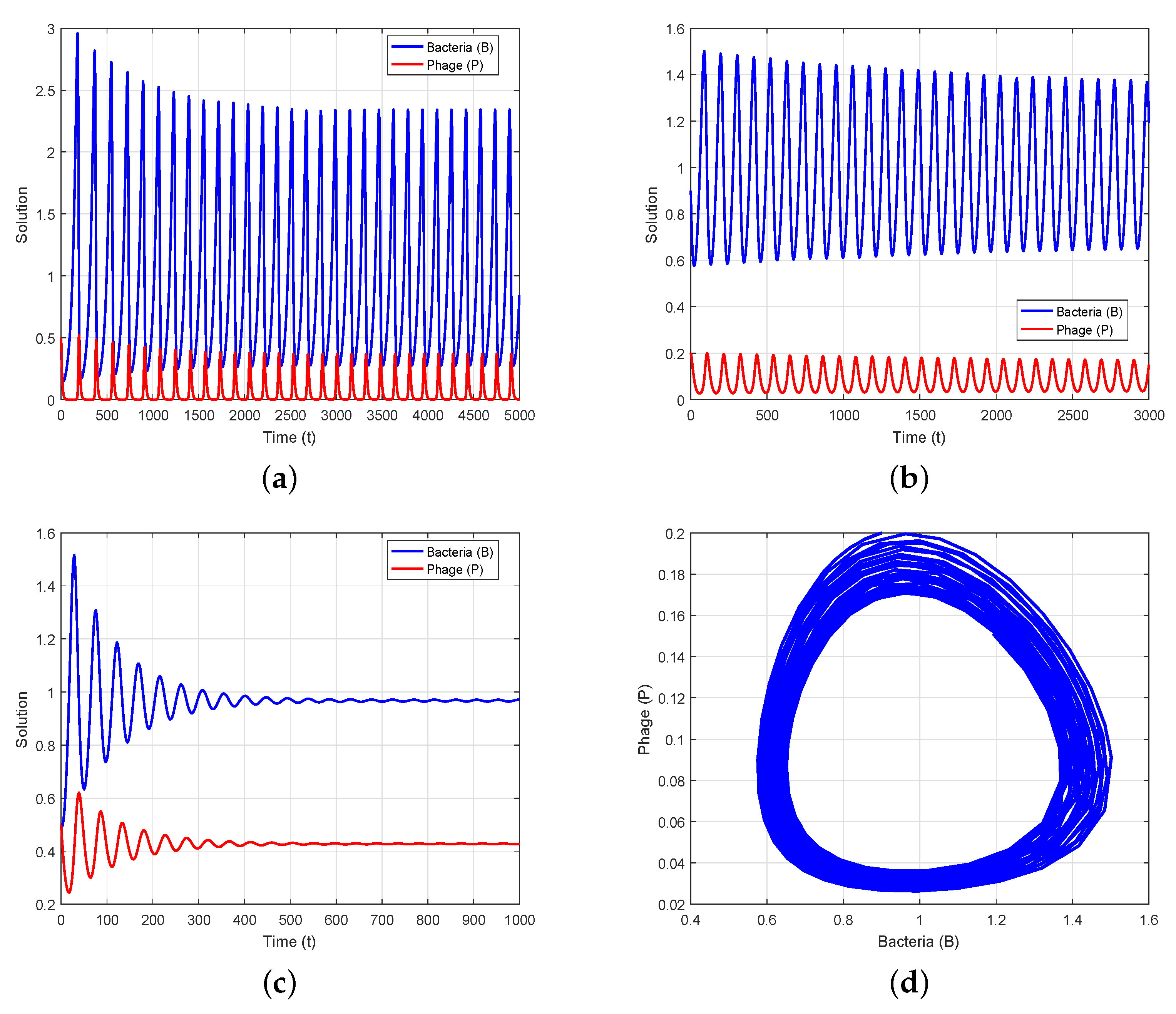
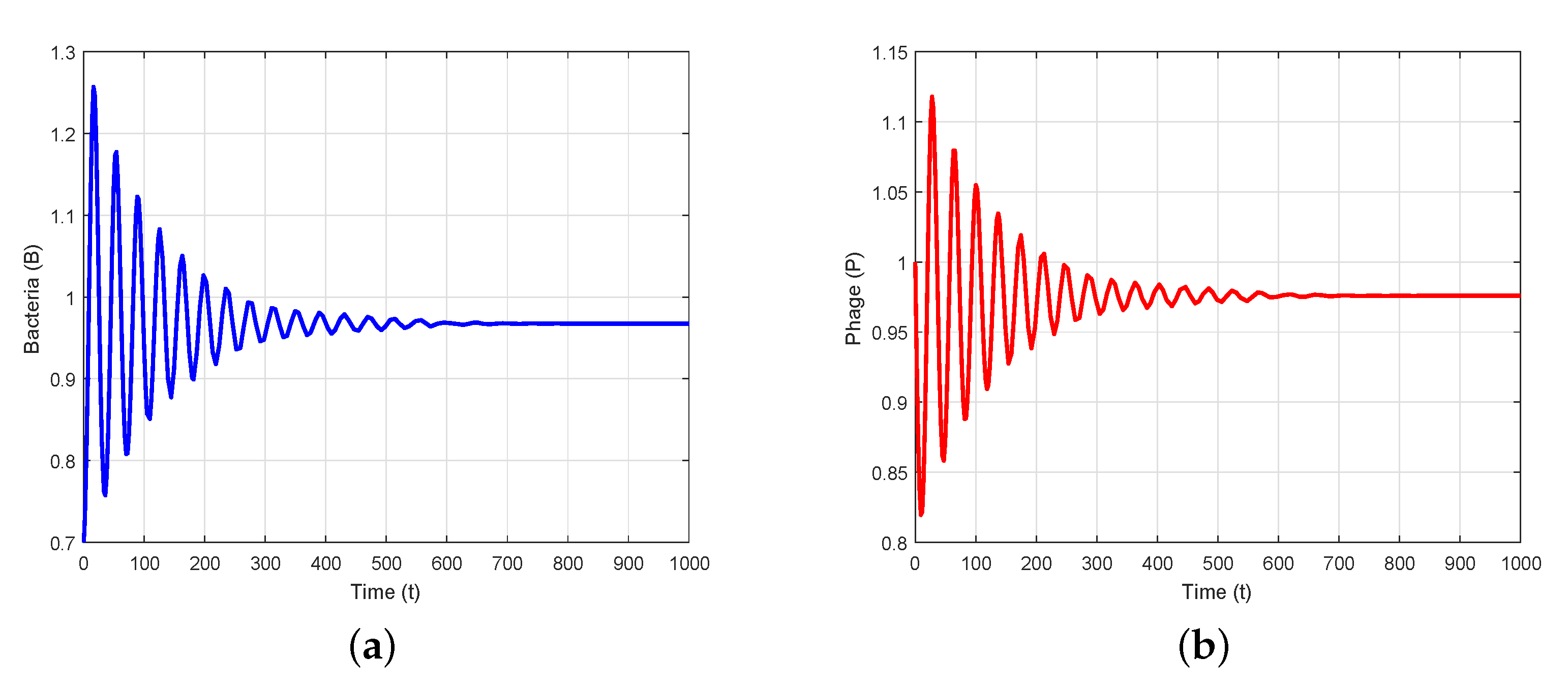
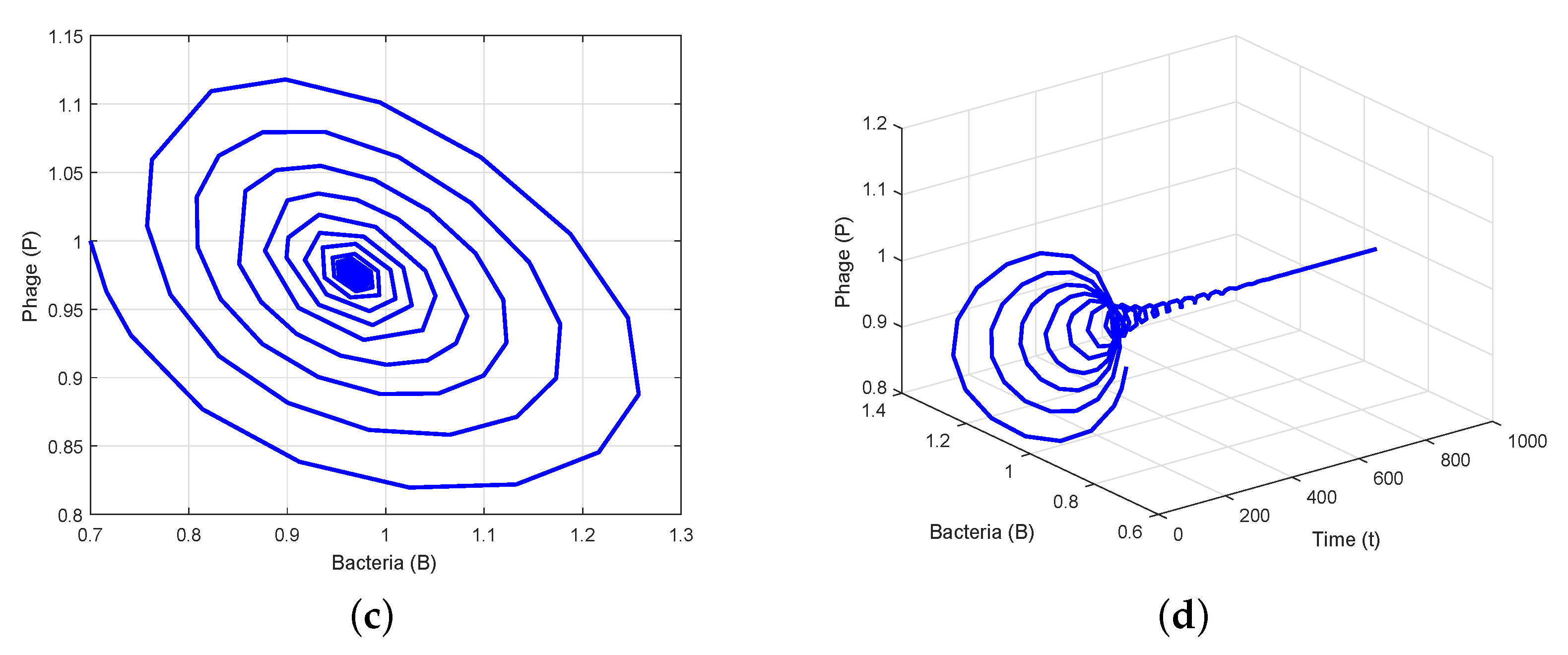
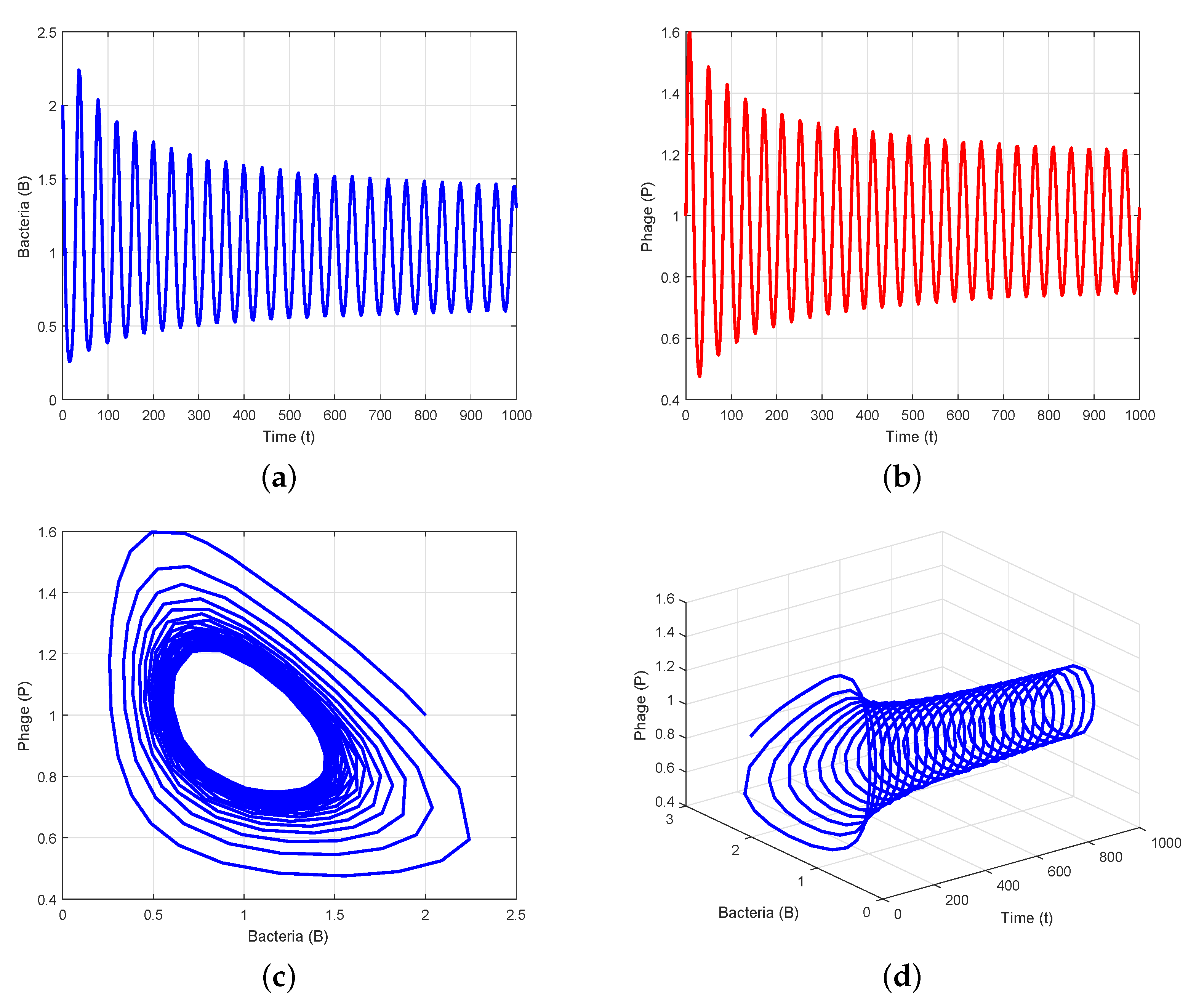
4. Numerical Simulation

In this section, we validate the theoretical outcomes through numerical simulations. We consider biologically feasible data in order to demonstrate the analytical outcomes, and the parameters are chosen as mentioned in

Table 1. Parameter interpretations and their values used in numerical simulations.

Parameter	Description	Data 1	Data 2
$\varphi$	adsorption rate of phage	0.34	0.34
$\beta$	burst size of phage	0.38	0.38
$ϵ$	killing rate of innate immune response	0.19	0.19
w	decay rate of phage	0.125	0.125
r	intrinsic growth rate of bacteria	0.25	0.5
$K_C$	carrying capacity of bacteria	7.29	5
$K_D$	bacterial concentration when innate immune
	response is half saturated	3.5	3.5
$K_I$	carrying capacity of innate immune response	0.48	0.48

.

We take the set of parameter values in Data 1 of Table 1 to correspond to the non-delayed System (2). For this dataset, the positive equilibrium is $E_2=(0.9675,0.4276)$. We derive $c_{11}+c_{22}=-0.0177<0$ and $c_{11}{c}_{22}-c_{12}{c}_{21}=0.0182>0$, which means that the system is locally asymptotically stable (LAS) around $E_2$. It can be seen that $E_2$ is stable using the first condition of Theorem 3(i). To analyze the existence of Hopf bifurcation in the case of a non-delayed system, we consider the parameter r as a bifurcation parameter and obtain the value of r as $r^{\ast }=0.1166$ with the same set of parameters stated in Data 1. We can deduce from the second condition of Theorem 3(i) that the positive equilibrium $E_2$ is destabilized by a Hopf bifurcation when $r=0.109<r^{\ast }$ (Figure 1a). According to Theorem 3(ii), System (2) undergoes a Hopf bifurcation at $E_2$ when r passes $r^{\ast }$ (Figure 1b), resulting in a stable limit cycle (Figure 1d). In Figure 1c, taking $r=0.25>r^{\ast }$, we conclude from Theorem 3(i) that $E_2$ is stable.

To verify the theoretical analysis outcomes in the delayed system (3), we consider the set of parameter values in Data 2 of Table 1. Using these parameter values, we obtain positive equilibrium $E_2(B^{\ast },P^{\ast })=(0.9675,0.9759)$ and compute $c_1=0.2063$, $c_2=0.0102$, $c_3=-0.1250$, and $c_4=0.0313$. Furthermore, we compute ${\omega }_0=0.1628$ and ${\tau }_0=3.3270$ using (25) and (27). Thus, we can demonstrate the transversality condition of Hopf bifurcation $\Phi =\mathrm{sign}{\left[\mathrm{Re}{\left(\frac{d\lambda }{d\tau }\right)}^{-1}\right]}_{\lambda =i{\omega }_0}=42.7388>0$ at the critical value of $\tau ={\tau }_0=3.3270$. According to Theorem 7(i), the positive equilibrium $E_2(B^{\ast },P^{\ast })$ is stable when $\tau <{\tau }_0=3.3270$ (Figure 2). Theorem 7(iii) leads us to deduce that System (3) exhibits a Hopf bifurcation at $E_2=(0.9675,0.9759)$ when $\tau ={\tau }_0=3.3270$, i.e., there is a periodic solution around $E_2=(0.9675,0.9759)$ when $\tau$ is close to ${\tau }_0=3.3270$ (Figure 3). When we determine the value of $\tau$ as $\tau =3.5>{\tau }_0=3.3270$, then $E_2(B^{\ast },P^{\ast })$ is unstable through a Hopf bifurcation and periodic orbits are encountered, as depicted in Figure 4. Figure 5 displays the phase portrait for various $\tau$ values, with $\tau ={\tau }_0=3.9$ and $\tau ={\tau }_0=5.5$ producing stable limit cycles.

5. Conclusions

In this paper, we modify and analyze the phage therapy model in (2) by including a discrete time delay to obtain its delayed version in (3). This modification is carried out by adding a discrete time delay to the recruitment term of the phages and the infection term of the bacteria. We investigate the dynamic behaviors of the models in (2) and (3), in particular in terms of their stability and Hopf bifurcation. In addition, we examine the Hopf bifurcation properties of System (3), including the bifurcation direction and the stability of a bifurcating periodic solution. Finally, numerical simulations are provided to prove the practical use of the theoretical results.

We consider the positivity and boundedness of both non-delayed and delayed models. The results demonstrate that all of the system’s solutions are positive and bounded, indicating that the system is biologically well-behaved.

For the non-delayed model, we explore the necessary conditions for the local stability of all equilibrium solutions and the occurrence of Hopf bifurcation, taking the bacterial intrinsic growth rate r as a bifurcation parameter. In Section 2, the Hopf bifurcation of this model is investigated using Hopf bifurcation theory; it is proved that there exists a critical value of $r^{\ast }$ for stability. When the value of r passes through the critical value of $r^{\ast }$, the system loses its stability and Hopf bifurcation occurs. This suggests that the intrinsic growth rate of bacteria has a stabilizing effect on the dynamics of the system.

In Section 4, we demonstrate numerically that the non-delayed System (2) encounters Hopf bifurcation when the parameter r passes a critical value $r^{\ast }$ (Figure 1b,d). When the value of r is gradually increased, the positive equilibrium $E_2$ reaches stability from instability. (Figure 1a,c). The results of our numerical simulations used to depict the analytical results are based on biologically feasible data.

We use the Lyapunov functional method to derive the global stability criteria for the boundary and coexistence equilibrium points in the non-delayed model. The results indicate that the phage burst size $\beta$ significantly affects the global stability behaviour of the coexistence equilibrium in the phage therapy model. The necessary conditions for the non-existence of periodic solutions to the system are established using the Dulac–Bendixon criterion. This result can be biologically explained as follows: if the bacterial growth rate is greater than the threshold value, then System (2) has no limit cycle.

In the second part of this study, we investigate the system’s dynamic behaviour in the presence of a time delay. We use the discrete delay as a bifurcation parameter in the Hopf bifurcation analysis to capture the oscillatory behaviour of the delayed model in (3). In Section 3, using stability theory and Hopf bifurcation theory, the influence of delay on the stability of the equilibrium point is studied along with the existence of Hopf bifurcation. Theorems for the stability and existence of Hopf bifurcation are established. The results show that the time delay destabilizes the system, leading to species coexistence.

It can be inferred from Theorem 7 that Hopf bifurcation arises in System (3) at the critical value $\tau ={\tau }_0$. When the value of $\tau$ is increased to ${\tau }_0=3.3270$, the system loses stability and undergoes Hopf bifurcation (Figure 3). When $\tau >{\tau }_0$, System (3) enters an unstable equilibrium via Hopf bifurcation at the interior equilibrium $E_2$, indicating that the densities of bacteria and phages oscillate periodically (Figure 4). However, the system achieves a stable equilibrium state when $\tau <{\tau }_0$, indicating that the densities of bacteria and phages tend towards a steady state (Figure 2). Our research indicates that oscillatory behavior is feasible in certain circumstances and that a delay can cause a stable equilibrium to evolve into an unstable one.

Furthermore, the direction and stability of the bifurcating periodic solutions are derived by applying normal form theory and the center manifold theorem. Based on Theorem 8, we obtain the formulas for determining the attributes of the Hopf bifurcation of the system. In particular, the Hopf bifurcation is supercritical and the bifurcating periodic solutions are stable under certain conditions.

In summary, this paper has shown that the addition of delay can destabilize the system and induce Hopf bifurcation. These results are in agreement with the destabilization effect that has been observed in previous models when introducing a time delay. From a biomedical perspective, this means that bacteria and phages can coexist under certain conditions if the delay required for phage reproduction and bacterial infection is small or increases to a critical value. This result has a significant effect on determining the most suitable time to introduce phage therapy.

Stochastic differential equations (SDEs) have become popular in modeling ecological and epidemiological models such as the study of population growth and epidemic transmission, as population dynamics vary concern with random perturbation. Population individuals struggle with one another for a restricted amount of nourishment and dwelling space. Environmental noise frequently influences population systems; therefore, it is crucial to determine whether this noise has an impact on the results. As far as we know, the phage therapy population model in (1) has not been studied yet with regard to its stochastic perturbation and asymptotic behavior. Therefore, in the future we intend to consider the behavior of the phage therapy model with stochastic perturbation in order to investigate the impact of random perturbations on model dynamics.

References

1. Beke, G.; Stano, M.; Klucar, L. Modeling the interaction between bacteriophages and their bacterial hosts. Math. Biosci. 2016, 279, 27–32. [Google Scholar] [CrossRef] [PubMed]
2. Beretta, E.; Kuang, Y. Modeling and analysis of a marine bacteriophage infection. Math. Biosci. 1998, 149, 57–76. [Google Scholar] [CrossRef]
3. Clokie, M.R.J.; Millard, A.D.; Letarov, A.V.; Heaphy, S. Phages in nature. Bacteriophage 2011, 1, 31–45. [Google Scholar] [CrossRef] [PubMed]
4. Sinha, S.; Grewal, R.K.; Roy, S. Modeling bacteria-phage interactions and its implications for phage therapy. Adv. Appl. Microbiol. 2018, 103, 103–141. [Google Scholar]
5. Brives, C.; Pourraz, J. Phage therapy as a potential solution in the fight against AMR: Obstacles and possible futures. Palgrave Commun. 2020, 6, 100. [Google Scholar] [CrossRef]
6. Styles, K.M.; Brown, A.T.; Sagona, A.P. A review of using mathematical modeling to improve our understanding of bacteriophage, bacteria, and eukaryotic interactions. Front. Microbiol. 2021, 2021, 2752. [Google Scholar] [CrossRef]
7. Al-Darabsah, I. Time Delayed Models in Population Biology and Epidemiology. Ph.D. Dissertation, Memorial University of Newfoundland, St. John’s, NL, Canada, 2018. [Google Scholar]
8. Campbell, A. Conditions for the existence of bacteriophage. Evolution 1961, 15, 153–165. [Google Scholar] [CrossRef]
9. Levin, B.R.; Stewart, F.M.; Chao, L. Resource-limited growth, competition, and predation: A model and experimental studies with bacteria and bacteriophage. Am. Nat. 1977, 111, 3–24. [Google Scholar] [CrossRef]
10. Lenski, R.E.; Levin, B.R. Constraints on the coevolution of bacteria and virulent phage: A model, some experiments, and predictions for natural communities. Am. Nat. 1985, 125, 585–602. [Google Scholar] [CrossRef]
11. Smith, H.L.; Trevino, R.T. Bacteriophage infection dynamics: Multiple host binding sites. Math. Model. Nat. Phenom. 2009, 4, 109–134. [Google Scholar] [CrossRef]
12. Sahani, S.K.; Gakkhar, S. A mathematical model for phage therapy with impulsive phage dose. Differ. Equ. Dyn. Syst. 2020, 28, 75–86. [Google Scholar] [CrossRef]
13. Smith, H.L. Models of virulent phage growth with application to phage therapy. SIAM J. Appl. Math. 2008, 68, 1717–1737. [Google Scholar] [CrossRef]
14. Misra, A.K.; Gupta, A.; Venturino, E. Cholera dynamics with bacteriophage infection: A mathematical study. Chaos Solitons Fract. 2016, 91, 610–621. [Google Scholar] [CrossRef]
15. Teytsa, H.M.N.; Tsanou, B.; Bowong, S.; Lubuma, J.M. Bifurcation analysis of a phage-bacteria interaction model with prophage induction. Math. Med. Biol. 2021, 38, 28–58. [Google Scholar] [CrossRef]
16. Li, X.; Huang, R.; He, M. Dynamics model analysis of bacteriophage infection of bacteria. Adv. Differ. Equ. 2021, 488, 3–11. [Google Scholar] [CrossRef]
17. Xu, C.; Tang, X.; Liao, M. Stability and bifurcation analysis of a delayed predator-prey model of prey dispersal in two-patch environments. Appl. Math. Comput. 2010, 216, 2920–2936. [Google Scholar] [CrossRef]
18. Liu, Q.; Xu, R. Stability and bifurcation of a Cohen-Grossberg neural network with discrete delays. Appl. Math. Comput. 2011, 218, 2850–2862. [Google Scholar] [CrossRef]
19. Li, Y.; Li, C. Stability and Hopf bifurcation analysis on a delayed Leslie–Gower predator-prey system incorporating a prey refuge. Appl. Math. Comput. 2013, 219, 4576–4589. [Google Scholar] [CrossRef]
20. Khajanchi, S.; Banerjee, S. Stability and bifurcation analysis of delay induced tumor immune interaction model. Appl. Math. Comput. 2014, 248, 652–671. [Google Scholar] [CrossRef]
21. Beretta, E.; Kuang, Y. Modeling and analysis of a marine bacteriophage infection with latency period. Nonlinear Anal. Real World Appl. 2001, 2, 35–74. [Google Scholar] [CrossRef]
22. Beretta, E.; Solimano, F. The effect of time delay on stability in a bacteria-bacteriophage model. Sci. Math. Jpn. 2003, 58, 399–405. [Google Scholar]
23. Liu, S.; Liu, Z.; Tang, J. A delayed marine bacteriophage infection model. Appl. Math. Lett. 2007, 20, 702–706. [Google Scholar] [CrossRef]
24. Gakkhar, S.; Sahani, S.K. A time delay model for bacteria bacteriophage interaction. J. Biol. Syst. 2008, 16, 445–461. [Google Scholar] [CrossRef]
25. Smith, H.L.; Thieme, H.R. Persistence of bacteria and phages in a chemostat. J. Math. Biol. 2012, 64, 951–979. [Google Scholar] [CrossRef]
26. Aviram, I.; Rabinovitch, A. Bifurcation analysis of bacteria and bacteriophage coexistence in the presence of bacterial debris. Commun. Nonlinear Sci. Numer. Simul. 2012, 17, 242–254. [Google Scholar] [CrossRef]
27. Calsina, A.; Palmada, J.M.; Ripoll, J. Optimal latent period in a bacteriophage population model structured by infection-age. Math. Model. Methods Appl. Sci. 2011, 21, 693–718. [Google Scholar] [CrossRef]
28. Aviram, I.; Rabinovitch, A. Bacteria and lytic phage coexistence in a chemostat with periodic nutrient supply. Bull. Math. Biol. 2014, 76, 225–244. [Google Scholar] [CrossRef]
29. Han, Z.; Smith, H.L. Bacteriophage-resistant and bacteriophage-sensitive bacteria in a chemostat. Math. Biosci. Eng. 2012, 9, 737–765. [Google Scholar]
30. Beretta, E.; Solimano, F.; Tang, Y.B. Analysis of a chemostat model for bacteria and virulent bacteriaphage. Discrete Cont. Dyn. Syst. Ser. B 2002, 2, 495–520. [Google Scholar]
31. Beretta, E.; Sakakibara, H.; Takeuchi, Y. Stability analysis of time delayed chemostat models for bacteria and virulent phage. Dyn. Syst. Their Appl. Biol. 2003, 36, 45–58. [Google Scholar]
32. Czárxaxn, T.; Rattray, F.P.; Möller, C.O.A.; Christensen, B.B. Modelling the influence of metabolite diffusion on non-starter lactic acid bacteria growth in ripening cheddar cheese. Int. Dairy J. 2018, 80, 35–45. [Google Scholar]
33. Wang, J.; Zheng, H.; Jia, Y. Dynamical analysis on a bacteria-phages model with delay and diffusion. Chaos Solitons Fract. 2021, 143, 110597. [Google Scholar] [CrossRef]
34. Gourley, S.A.; Kuang, Y. A delay reaction-diffusion model of the spread of bacteriophage infection. SIAM J. Appl. Math. 2005, 65, 550–566. [Google Scholar] [CrossRef]
35. Carletti, M. On the stability properties of a stochastic model for phage bacteria interaction in open marine environment. Math. Biosci. 2002, 175, 117–131. [Google Scholar] [CrossRef]
36. Carletti, M. Mean-square stability of a stochastic model for bacteriophage infection with time delays. Math. Biosci. 2007, 210, 395–414. [Google Scholar] [CrossRef]
37. Bardina, X.; Bascompte, D.; Rovira, C.; Tindel, S. An analysis of stochastic model for bacteriophage systems. Math. Biosci. 2013, 241, 99–108. [Google Scholar] [CrossRef] [PubMed]
38. Vidurupola, S.W.; Allen, L.J.S. Impact of Variability in Stochastic Models of Bacteria-Phage Dynamics Applicable to Phage Therapy. Stoch. Anal. Appl. 2014, 32, 427–449. [Google Scholar] [CrossRef]
39. Vidurupola, S.W. Analysis of deterministic and stochastic mathematical models with resistant bacteria and bacteria debris for bacteriophage dynamics. Appl. Math. Comput. 2018, 316, 215–228. [Google Scholar] [CrossRef]
40. Abedon, S.T.; Kuhl, S.J.; Blasdel, B.G.; Kutter, E.M. Phage treatment of human infections. Bacteriophage 2011, 1, 66–85. [Google Scholar] [CrossRef]
41. Cisek, A.A.; Dabrowska, I.; Gregorczyk, K.P.; Wyzewski, Z. Phage therapy in bacterial infections treatment: One hundred years after the discovery of bacteriophages. Curr. Microbiol. 2017, 74, 277–283. [Google Scholar] [CrossRef]
42. Leung, C.Y.; Weitz, J.S. Modeling the synergistic elimination of bacteria by phage and the innate immune system. J. Theor. Biol. 2017, 429, 241–252. [Google Scholar] [CrossRef] [PubMed]
43. Kyaw, E.E.; Zheng, H.; Wang, J.; Hlaing, H.K. Stability analysis and persistence of a phage therapy model. Math. Biosci. Eng. 2021, 18, 5552–5572. [Google Scholar] [CrossRef] [PubMed]
44. Birkhoff, G.; Rota, G.C. Ordinary Differential Equations; John Wiley and Sons: New York, NY, USA, 1982. [Google Scholar]
45. Tripathi, J.P.; Tyagi, S.; Abbas, S. Global analysis of a delayed density dependent predator-prey model with Crowley-Martin functional response. Commun. Nonlinear Sci. Numer. Simul. 2016, 30, 45–69. [Google Scholar] [CrossRef]
46. Perko, L. Differential Equations and Dynamical Systems; Springer Science and Business Media: Berlin/Heidelberg, Germany, 2001. [Google Scholar]
47. Freedman, H.I.; Rao, V.S.H. The trade-off between mutual interference and time lags in predator-prey ststems. Bull. Math. Biol. 1983, 45, 991–1004. [Google Scholar] [CrossRef]
48. Wiggins, S. Introduction to Applied Nonlinear Dynamical Systems and Chaos; Springer: New York, NY, USA, 1990. [Google Scholar]
49. Kuang, Y. Delay Differential Equation with Applications in Population Dynamics; Academic Press: New York, NY, USA, 1993. [Google Scholar]
50. Hassard, B.D.; Kazarinoff, N.D.; Wan, Y.H. Theory and Applications of Hopf Bifurcation; University Cambridge: Cambridge, UK, 1981. [Google Scholar]
Figure 1. Oscillatory behavior of System (2) with parameter values stated in Data 1 except for r: (a) Unstable solution of system when r = 0.109 < r ; (b) existence of Hopf bifurcation solution for r = r = 0.1166 ; (c) stable solution of system when r = 0.25 > r ; (d) existence of a stable limit cycle near E 2 when r = r .
Axioms 12 00772 g001
Figure 2. E 2 is asymptotically stable when τ = 2.3 < τ 0 : (a,b) time series evolution of bacteria and phages; (c) phase portrait in B-P plane; (d) phase portrait in t-B-P space.
Axioms 12 00772 g002aAxioms 12 00772 g002b
Figure 3. Existence of Hopf bifurcation solution for τ = 3.3270 = τ 0 around E 2 : (a,b) time series evolution of bacteria and phages; (c) presence of a stable limit cycle; (d) phase portrait in t-B-P space.
Axioms 12 00772 g003
Figure 4. E 2 is unstable when τ = 3.5 > τ 0 : (a,b) time series evolution of bacteria and phages; (c) presence of periodic solution; (d) phase portrait in t-B-P space.
Axioms 12 00772 g004
Figure 5. Phase portraits for various values of time delays: (a) a stable limit cycle emerges at τ = 3.9 due to Hopf bifurcation; (b) a stable limit cycle emerges at τ = 5.5 due to Hopf bifurcation, resulting in stable periodic solutions.
Axioms 12 00772 g005