Minor and Major Strain: Equations of Equilibrium of a Plane Domain with an Angular Cutout in the Boundary

Abstract

Large values and gradients of stress and strain, triggering concentrated stress and strain, arise in angular areas of a structure. The strain action, leading to the finite loss of contact between structural elements, also triggers concentrated stress. The loss of contact reaches an irregular point and a line on the boundary. The theoretical analysis of the stress–strain state (SSS) of areas with angular cutouts in the boundary under the action of discontinuous strain is reduced to the study of singular solutions to the homogeneous problem of elasticity theory with power-related features. The calculation of stress concentration coefficients in the domain of a singular solution to the elastic problem makes no sense. It is experimentally proven that the area located near the vertex of an angular cutout in the boundary features substantial strain and rotations, and it corresponds to higher values of the first and second derivatives of displacements along the radius in cases of sufficiently small radii in the neighborhood of an irregular boundary point. As far as these areas are concerned, it is necessary to consider the plane problem of the elasticity theory, taking into account the geometric nonlinearity under the action of strain, to analyze the effect of relationships between strain orders, rotations, and strain on the form of the equation of equilibrium. The purpose of this work is to analyze the effect of relationships between strain orders, rotations, and strain on the form of the equilibrium equation in the polar system of coordinates for a V-shaped area under the action of temperature-induced strain, taking into account geometric non-linearity and physical linearity.

1. Introduction

Structures with angular boundary areas are characterized by large values and gradients of stress and strain. Theoretical studies of areas with angular cutouts in the boundary are reduced to singular solutions to homogeneous boundary problems of model areas that are V-shaped and cone-shaped. The singularity of the solution in the area of the angular cutout in the boundary is determined by the idealization of the mathematical formulation of the boundary value problem of the theory of elasticity [1,2,3,4,5,6,7,8,9,10,11,12,13,14]. The calculation of concentration coefficients as relative values is not possible in such areas.

Figure 1 shows interference fringes for a plane model with different angles of cutouts in the boundary.

An experimental solution to the elastic problem of strain is illustrated for the plane domain through the case of a composite plane model that is 180 mm long and 24 mm wide. Deformation defrosting and photo-elasticity methods are employed to obtain the experimental solution [15,16,17,18,19,20].

Temperature-induced strain $\mathsf{\alpha }T{\mathsf{\delta }}_{ij}$ is created in one part of model ${\mathsf{\Omega }}_2$, while the other part, ${\mathsf{\Omega }}_1$, remains unloaded. A spike in temperature-induced strain along the contact surface reaches irregular boundary point O (0,0), which is the vertex of the cutout. Different patterns of fringes are obtained for different angles of the cutout in the boundary (Figure 1).

It has been experimentally proven [15,16,17,18,19,20] that substantial strain and rotations are observed in the area close to the vertex of the angular cutout in the boundary area, which corresponds to higher values of the first and second derivatives of displacements along the radius if the radii in the neighborhood of the irregular boundary point are small enough. The plane problem of elasticity theory must be considered for such areas, taking into account geometric nonlinearity under the action of strain.

General methods used to solve problems of solid mechanics, based on a solution to the nonlinear problem of the elasticity theory, were developed in the fundamental works of V.V. Novozhilov [21,22], P.A. Lukash [23], and A.I. Lurie [24], and in other works [25,26,27,28,29]. Geometric relationships, containing square terms, are used in the nonlinear elasticity theory. Equilibrium equations are formulated as the post-strain equilibria of an oblique parallelepiped [21,22,27,28].

Physical and geometric relations, addressed by problems of the theory of elasticity, can be interpreted as:

(A)

Physically and geometrically linear;

(B)

Physically linear and geometrically nonlinear;

(C)

Physically nonlinear and geometrically linear;

(D)

Physically and geometrically nonlinear.

This paper considers the domain in which linear physical relations are applicable to strain and stress, while geometrically nonlinear expressions are applicable to strain.

Nonlinear strain has squared strain parameters, including linear and shear parameters, rotations, and their products. In some cases, linear and shear strain values are small compared to rotations, or rotations are small compared to linear and shear strain values (classical linear geometric relations). Taking into account the nonlinearity of geometric relations, the analysis of possible relations between orders of linear strain, shear, rotations, and pre-set strain becomes more complicated and requires detailed consideration.

Displacements are continuous together with their partial derivative coordinate functions within the domain.

The possibility of the linearization of (a) relations between strain and displacements and (b) equations of equilibrium of a spatial element is characterized by the geometric factor; that is, the value of elongations, shear, and rotations in comparison with one and in comparison with each other.

Equilibrium equations and geometric relations do not depend on mechanical properties of the medium. Geometric relations deal with the measurement unit of elongation, taken as the ratio of a change in the length of a segment in case of strain in the domain to its original length. The types of equations of equilibrium and geometric relations depend on relations between values of strain parameters.

As for physical relations, the phenomenological approach is applied to establish relationships between nonlinear strain and generalized stress [21,22,27].

The concept of generalized stress is introduced in the works of V.V. Novozhilov. He assumes that it is not stress according to its classical definition. Expressions of generalized stress take into account a change in the geometry, or areas of faces in case of the deformation of an element of an elastic body. V.V. Novozhilov argues that the following three functions are sufficient to describe the mechanical properties of an ideally elastic, geometrically nonlinear isotropic medium [21,22]: K* is the generalized modulus of dilatation; G* is the generalized shear modulus; and ${\omega }^{*}$ is the phase of similarity of stress and strain deviators.

The author assumes that ${\omega }^{*}$ = 0, and this assumption determines the proportionality between stress and strain components. Linear physical relations are formulated for generalized stress and nonlinear strain. For an isotropic homogeneous body, generalized characteristics K*, G*, and ${\omega }^{*}$ are assumed to be constant, which corresponds to Lame’s constant mechanical parameters or the modulus of elasticity and the Poisson’s ratio.

Geometrically nonlinear relations and linear physical relations for generalized stress and strain are applicable to the domain where these relations are valid.

Nonlinear strain expressions and linear relations between generalized stress and strain are used to obtain equations of equilibrium in case of strain. To obtain such equations, it is necessary to make a mathematical model that simulates nonlinear geometric relations, equations of statics for the deformed scheme, and applications of the phenomenological approach to physical relations in the case of constant generalized mechanical characteristics.

The experimental data, obtained using the photo-elasticity method [15,16,17,18,19], show that areas with small strain and areas with large stress and strain gradients are identified in the area of an angular cutout in the boundary.

The purpose of this research is to analyze the effect of relations of orders of strain, and rotations on the form of the equilibrium equation in the polar system of coordinates for the V-shaped area under the action of forced, temperature-induced strain with regard to geometric nonlinearity and physical linearity.

The objectives of this research undertaking are:

(1)

To formulate equilibrium equations for the deformed scheme and obtain equilibrium equations for cases of generalized stress and strain in the plane domain, taking into account geometric nonlinearity and physical linearity;

(2)

To formulate equilibrium equations for the deformed scheme in terms of possible relations of orders of linear strain, shear, and angles of rotation, and to analyze the effect of relations of strain orders on the form of equilibrium equations.

2. Materials and Methods

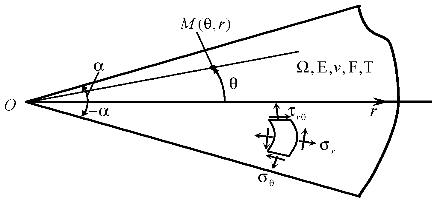
2.1. Problem Statement

The elasticity theory problem is considered for a plane domain with an irregular boundary point, or the vertex of an angular cutout. Forced–free temperature-induced strain $\alpha T{\delta }_{ij}$, where ${\delta }_{ij}$ is the Kronecker symbol, is pre-set in the plane domain $\mathsf{\Omega }$ (Figure 2). In the domain $\mathsf{\Omega }={\mathsf{\Omega }}_1\cup {\mathsf{\Omega }}_2$, a spike (the finite rupture) in strain along the line of contact between domains $\mathsf{\Gamma }={\mathsf{\Omega }}_1\cap {\mathsf{\Omega }}_2$, extending to the vertex of the angular cutout, can be pre-set. For example, the strain discontinuity is triggered if one of the subdomains ${\mathsf{\Omega }}_2$ of the $\mathsf{\Omega }={\mathsf{\Omega }}_1\cup {\mathsf{\Omega }}_2$ domain is subjected to pre-set temperature-induced strain $\alpha T{\delta }_{ij}$ while the second subdomain ${\mathsf{\Omega }}_1$ is not loaded. Volumetric forces can be pre-set in the plane domain $\mathsf{\Omega }$. Concentrated forces are not considered. A homogeneous elastic body is in the state of plane deformation [3,6,29]. Mechanical characteristics include modulus of elasticity E and Poisson’s coefficient $\nu$; they are constant in the $\mathsf{\Omega }$ domain. Linear expansion coefficient $\alpha$ in the $\mathsf{\Omega }$ domain is constant. Boundary conditions for stress are homogeneous.

Let us consider the polar system of coordinates with the pole of the polar system O (0,0) at the vertex of the angular cutout. Let displacement, strain, and stress functions and their derivatives be continuous everywhere in the domain $\mathsf{\Omega }$, except for the vertex of the angular cutout. If there is a discontinuity of strain along the contact line of domains $\mathsf{\Gamma }={\mathsf{\Omega }}_1\cap {\mathsf{\Omega }}_2$, then continuity conditions are fulfilled for displacements and normal stresses along the contact line of the domains. The vertex of the angular is removed, and its punctured neighborhood in the domain $\mathsf{\Omega }$ is considered.

Different relations for orders of strain values are considered depending on the approximation to the irregular boundary point, in order to determine different kinds of solving systems for equations of the elastic boundary value problem.

The objective is to formulate equations of equilibrium in the domain $\mathsf{\Omega }$, taking into account geometric nonlinearity and physical linearity.

2.2. Equilibrium Equations

A spatial curvilinear orthogonal system of coordinates [17,21,22] ${\alpha }_i$ is considered; i = 1,2,3, ${\overrightarrow{k}}_i$ are unitary vectors pointed toward the positive direction of ${\alpha }_i$ axes or basis vectors of the domain before the strain action. An infinitesimal element is identified. This element is limited by six coordinate planes; before the strain action, this element is a rectangular parallelepiped. Sizes and directions of edges are determined by vectors $H_i {\overrightarrow{k}}_i d{\alpha }_i$, where $H_i$ are the Lame’s parameters. After the strain action, a rectangular parallelepiped transforms into an oblique one. Sizes and directions of its edges are determined by vectors $H_i(1+E_{\alpha i}) {\overrightarrow{k}}_i^{*} d{\alpha }_i$, where $E_{\alpha i}$ are relative elongations along ${\alpha }_i$ axes after the strain action and ${\overrightarrow{k}}_i^{*}$ are basis vectors of the domain after the strain action.

Equations of equilibrium of all forces, acting on the oblique parallelepiped after the strain action [21,22,24], have the form

$$\frac{1}{H_1{H}_2{H}_3}\left\{\frac{\partial }{\partial {\alpha }_1}(H_2{H}_3{\overrightarrow{\sigma }}_{n_1}^{*})+\frac{\partial }{\partial {\alpha }_2}(H_3{H}_1{\overrightarrow{\sigma }}_{n_2}^{*})+\frac{\partial }{\partial {\alpha }_3}(H_1{H}_2{\overrightarrow{\sigma }}_{n_3}^{*})\right\}+\overrightarrow{F}=0,$$

(1)

where ${\overrightarrow{\sigma }}_{ni}^{*}={\overrightarrow{\sigma }}_{ni} S_i^{*}/S_i$ are generalized stresses, arising on the edges of the oblique parallelepiped; $S_i^{*}, S_i$ are the areas of edges of the parallelepiped after and before the strain action; and $\overrightarrow{F}$ are generalized volumetric forces after the strain action.

Geometric relations and static equations are formulated in two different systems of coordinates. Therefore, from the beginning, equations of equilibrium obtained for the element after the strain action are formulated in the system of coordinates before the strain action: ${\overrightarrow{\sigma }}_{ni}^{*}=s_{1i}{\overrightarrow{k}}_1+s_{2i}{\overrightarrow{k}}_2+s_{3i}{\overrightarrow{k}}_3$.

Having formulated forces on the edges of the parallelepiped after the strain action within the initial basis of vectors ${\overrightarrow{k}}_i$ before the strain action, Equation (1) will be formulated as follows:

$$\begin{array}{l}(\frac{\partial }{\partial {\alpha }_1}(H_2{H}_3{s}_{11})+\frac{\partial }{\partial {\alpha }_2}(H_3{H}_1{s}_{12})+\frac{\partial }{\partial {\alpha }_3}(H_1{H}_2{s}_{31})+H_3\frac{\partial H_1}{\partial {\alpha }_2}{s}_{12}+H_2\frac{\partial H_1}{\partial {\alpha }_3}{s}_{13}-\\ -H_3\frac{\partial H_2}{\partial {\alpha }_1}{s}_{22}-H_2\frac{\partial H_3}{\partial {\alpha }_1}{s}_{33}+H_1{H}_2{H}_3{F}_1=0\end{array},$$

(2)

$$\begin{array}{l}\frac{\partial }{\partial {\alpha }_1}(H_2{H}_3{s}_{12})+\frac{\partial }{\partial {\alpha }_2}(H_3{H}_1{s}_{22})+\frac{\partial }{\partial {\alpha }_3}(H_1{H}_2{s}_{32})+H_1\frac{\partial H_2}{\partial {\alpha }_3}{s}_{23}+H_3\frac{\partial H_2}{\partial {\alpha }_1}{s}_{21}-\\ -H_1\frac{\partial H_3}{\partial {\alpha }_2}{s}_{33}-H_3\frac{\partial H_1}{\partial {\alpha }_2}{s}_{11}+H_1{H}_2{H}_3{F}_2=0\end{array},$$

(3)

$$\begin{array}{l}\frac{\partial }{\partial {\alpha }_1}(H_2{H}_3{s}_{13})+\frac{\partial }{\partial {\alpha }_2}(H_3{H}_1{s}_{23})+\frac{\partial }{\partial {\alpha }_3}(H_1{H}_2{s}_{33})+H_3\frac{\partial H_3}{\partial {\alpha }_1}{s}_{31}+H_1\frac{\partial H_3}{\partial {\alpha }_2}{s}_{32}-\\ -H_2\frac{\partial H_1}{\partial {\alpha }_3}{s}_{11}-H_1\frac{\partial H_2}{\partial {\alpha }_3}{s}_{22}+H_1{H}_2{H}_3{F}_3=0\end{array}.$$

(4)

Here, $F_i$ are projections of the generalized volumetric force on directions ${\overrightarrow{k}}_i, i=1,2,3$.

In relations (2)–(4), expressions $s_{ij}$ are formulated using generalized stresses ${\sigma }_{ij}^{*}$, strain parameters $e_{\mathrm{i}\mathrm{j}}$, and rotations ${\omega }_{\mathrm{i}}$:

$$\begin{array}{c}{s}_{11}={\sigma }_{11}^{\ast }(1+e_{11})+{\sigma }_{12}^{\ast }(\frac{1}{2}{e}_{12}-{\omega }_2)+{\sigma }_{13}^{\ast }(\frac{1}{2}{e}_{13}+{\omega }_2)\hspace{1em}{s}_{23}={\sigma }_{21}^{\ast }(\frac{1}{2}{e}_{13}-{\omega }_2)+{\sigma }_{22}^{\ast }(\frac{1}{2}{e}_{23}+{\omega }_1)+{\sigma }_{23}^{\ast }(1+e_{33})\\ s_{12}={\sigma }_{11}^{\ast }(\frac{1}{2}{e}_{12}+{\omega }_3)+{\sigma }_{12}^{\ast }(1+e_{22})+{\sigma }_{13}^{\ast }(\frac{1}{2}{e}_{23}-{\omega }_1)\hspace{1em}{s}_{31}={\sigma }_{31}^{\ast }(1+e_{11})+{\sigma }_{32}^{\ast }(\frac{1}{2}{e}_{12}-{\omega }_2)+{\sigma }_{33}^{\ast }(\frac{1}{2}{e}_{13}+{\omega }_2)\\ s_{13}={\sigma }_{11}^{\ast }(\frac{1}{2}{e}_{13}-{\omega }_2)+{\sigma }_{12}^{\ast }(\frac{1}{2}{e}_{23}+{\omega }_1)+{\sigma }_{13}^{\ast }(1+e_{33})\hspace{1em}{s}_{32}={\sigma }_{31}^{\ast }(\frac{1}{2}{e}_{12}+{\omega }_3)+{\sigma }_{32}^{\ast }(1+e_{22})+{\sigma }_{33}^{\ast }(\frac{1}{2}{e}_{23}-{\omega }_1)\\ s_{21}={\sigma }_{21}^{\ast }(1+e_{11})+{\sigma }_{22}^{\ast }(\frac{1}{2}{e}_{12}-{\omega }_2)+{\sigma }_{23}^{\ast }(\frac{1}{2}{e}_{13}+{\omega }_2)\hspace{1em}{s}_{33}={\sigma }_{31}^{\ast }(\frac{1}{2}{e}_{13}-{\omega }_2)+{\sigma }_{32}^{\ast }(\frac{1}{2}{e}_{23}+{\omega }_1)+{\sigma }_{33}^{\ast }(1+e_{33})\\ s_{22}={\sigma }_{21}^{\ast }(\frac{1}{2}{e}_{12}+{\omega }_3)+{\sigma }_{22}^{\ast }(1+e_{22})+{\sigma }_{23}^{\ast }(\frac{1}{2}{e}_{23}-{\omega }_1)\end{array}$$

(5)

By substituting (5) into Equations (2)–(4), one can obtain equations of equilibrium in the curvilinear orthogonal system of coordinates ${\alpha }_1, {\alpha }_2, {\alpha }_3$, with account taken of nonlinear strain for generalized stress and strain parameters (5).

Using the Cartesian system of coordinates to solve the plane problem for V-shaped domains is a challenge because basis vectors change when an element is strained. Curvilinear and polar (a special case) systems of coordinates are used to derive static equations for a deformed scheme. A plane problem of the elasticity theory [3,4,6,29] is considered for the state of plane deformation, when points of a body move in the planes that are perpendicular to the OZ axis:

$$u_1=u_1({\alpha }_1,{\alpha }_2,0), u_2=u_2({\alpha }_1,{\alpha }_2,0), u_3({\alpha }_1,{\alpha }_2,0)=0.$$

(6)

For the polar system of coordinates:

$${\alpha }_1=r, {\alpha }_2=\phi , {\alpha }_3=z.$$

(7)

Geometric Lame’s parameters are as follows:

$$H_1=1, H_2=r, H_3=1$$

(8)

Equilibrium Equations (2)–(4) will be formulated as follows:

$$\frac{\partial s_{11}}{\partial r}+\frac{1}{r}\frac{\partial s_{21}}{\partial \phi }+\frac{s_{11}-s_{22}}{r}+F_1=0,$$

(9)

$$\frac{1}{r}\frac{\partial s_{22}}{\partial \phi }+\frac{\partial s_{12}}{\partial r}+\frac{s_{12}+s_{21}}{r}+F_2=0,$$

(10)

where relations for generalized stresses (5) in Equations (9) and (10) will be changed as follows:

$$s_{11}={\sigma }_{11}^{*}(1+e_{11})+{\sigma }_{12}^{*}(\frac{1}{2}{e}_{12}-{\omega }_3),s_{22}={\sigma }_{22}^{*}(1+e_{22})+{\sigma }_{21}^{*}(\frac{1}{2}{e}_{12}+{\omega }_3),$$

(11)

$$s_{12}={\sigma }_{11}^{*}(\frac{1}{2}{e}_{12}+{\omega }_3)+{\sigma }_{12}^{*}(1+e_{22}), s_{21}={\sigma }_{21}^{*}(1+e_{11})+{\sigma }_{22}^{*}(\frac{1}{2}{e}_{12}-{\omega }_3).$$

(12)

Taking into account (11), (12), equations of equilibrium (9), (10) will be changed as follows:

$$\begin{array}{l}\frac{\partial }{\partial r}\left({\sigma }_{11}^{*}(1+e_{11})+{\sigma }_{12}^{*}(\frac{1}{2}{e}_{12}-{\omega }_3)\right)+\frac{1}{r}\frac{\partial }{\partial \phi }\left({\sigma }_{21}^{*}(1+e_{11})+{\sigma }_{22}^{*}(\frac{1}{2}{e}_{12}-{\omega }_3)\right)+\\ \hspace{1em}+\frac{1}{r}\left[{\sigma }_{11}^{*}(1+e_{11})+{\sigma }_{12}^{*}(\frac{1}{2}{e}_{12}-{\omega }_3)-{\sigma }_{22}^{*}(1+e_{22})-{\sigma }_{21}^{*}(\frac{1}{2}{e}_{12}+{\omega }_3)\right]+F_1=0\end{array},$$

(13)

$$\begin{array}{l}\frac{1}{r}\frac{\partial }{\partial \phi }\left({\sigma }_{21}^{*}(\frac{1}{2}{e}_{12}+{\omega }_3)+{\sigma }_{22}^{*}(1+e_{22})\right)+\frac{\partial }{\partial r}\left({\sigma }_{11}^{*}(\frac{1}{2}{e}_{12}+{\omega }_3)+{\sigma }_{12}^{*}(1+e_{22})\right)+\\ \hspace{1em}+\frac{1}{r}\left[{\sigma }_{11}^{*}(\frac{1}{2}{e}_{12}+{\omega }_3)+{\sigma }_{12}^{*}(1+e_{22})+{\sigma }_{21}^{*}(1+e_{11})+{\sigma }_{22}^{*}(\frac{1}{2}{e}_{12}-{\omega }_3)\right]+F_2=0\end{array},$$

(14)

where generalized stresses ${\sigma }_{\mathrm{i}\mathrm{j}}^{*}$ are related to stresses ${\sigma }_{\mathrm{i}\mathrm{j}}$ at a point in the domain: ${\sigma }_{\mathrm{i}\mathrm{j}}^{*}=\frac{S_{\mathrm{i}}^{*}}{S_{\mathrm{i}}}{\sigma }_{\mathrm{i}\mathrm{j}}, \mathrm{i},\mathrm{j}=1,2$.

The form of linear equilibrium equations for generalized stresses in the polar system of coordinates (9), (10) coincides with the form of equilibrium equations for the minor strain:

$$\frac{\partial {\sigma }_r}{\partial r}+\frac{1}{r}\frac{\partial {\tau }_{r\theta }}{\partial \theta }+\frac{{\sigma }_r-{\sigma }_{\theta }}{r}+F_1=0,$$

(15)

$$\frac{1}{r}\frac{\partial {\sigma }_{\theta \theta }}{\partial \theta }+\frac{\partial {\tau }_{r\theta }}{\partial r}+\frac{2{\tau }_{r\theta }}{r}+F_2=0.$$

(16)

Let us formulate equations of equilibrium (13), (14) for the strain.

2.3. Deformation Relations

General strain relations for the curvilinear orthogonal system of coordinates are considered in [21,22,24]. Let us derive nonlinear relations for strain in the polar system of coordinates [21,30]. Relative elongation $E_{MN}$ at an arbitrary point M of domain $\mathsf{\Omega }$ is as follows:

$$E_{MN}=\frac{d{s}^{*}-ds}{ds}=\frac{\left|M^{*}{N}^{*}\right|-\left|MN\right|}{\left|MN\right|},$$

(17)

where ds is the length of segment MN before the strain action; $d{s}^{*}$ is the length of the segment $M^{*}{N}^{*}$ obtained by displacing points M and N after the strain action.

The direct derivation of nonlinear geometric relations for an element in the polar system of coordinates is problematic, unlike the derivation in the Cartesian system of coordinates; hence, such relations are not addressed in research works.

Let us consider a homogeneous elastic body in the state of plane deformation, for which [3,17,29] is satisfied:

$$u_1=u_1(r,\phi ,0), u_2=u_2(r,\phi ,0), u_3=u_3(r,\phi ,0)=0,$$

$${\epsilon }_{33}=0, {\epsilon }_{13}={\epsilon }_{31}=0, {\epsilon }_{23}={\epsilon }_{32}=0, e_{13}=e_{31}=0, e_{23}=e_{32}=0, e_{33}=0, e_{33}=0,$$

(18)

$${\sigma }_{13}^{*}={\sigma }_{31}^{*}=0,\hspace{1em}{\sigma }_{23}^{*}={\sigma }_{32}^{*}=0.$$

Strain in the plane domain $\mathsf{\Omega }$ for this unit of elongation (17) can be formulated as follows:

$${\epsilon }_{11}=e_{11}+\frac{1}{2}\left[e_{11}^2+{(\frac{1}{2}{e}_{12}+{\omega }_3)}^2\right], {\epsilon }_{22}=e_{22}+\frac{1}{2}\left[e_{22}^2+{(\frac{1}{2}{e}_{21}-{\omega }_3)}^2\right],$$

(19)

$${\epsilon }_{12}={\epsilon }_{21}=e_{12}+e_{11}(\frac{1}{2}{e}_{12}-{\omega }_3)+e_{22}(\frac{1}{2}{e}_{12}+{\omega }_3).$$

(20)

Here, displacements $u_1, u_2$ are used to formulate strain parameters in the polar system of coordinates:

$$e_{11}=\frac{\partial u_1}{\partial r}, e_{22}=\frac{1}{r}\frac{\partial u_2}{\partial \phi }+\frac{1}{r}{u}_1, \frac{1}{2}{e}_{12}+{\omega }_3=\frac{\partial u_2}{\partial r},$$

(21)

$$e_{12}=e_{21}=r\frac{\partial }{\partial r}\left(\frac{u_2}{r}\right)+\frac{1}{r}\frac{\partial u_1}{\partial \phi }=\frac{\partial u_2}{\partial r}-\frac{u_2}{r}+\frac{1}{r}\frac{\partial u_1}{\partial \phi }, \frac{1}{2}{e}_{12}-{\omega }_3=\frac{1}{r}\frac{\partial u_1}{\partial \phi }-\frac{u_2}{r}.$$

(22)

Then, auxiliary expressions (11), (12) will be reformulated in terms of displacements:

$$s_{11}={\sigma }_{11}^{*}(1+\frac{\partial u_1}{\partial r})+{\sigma }_{12}^{*}(\frac{1}{r}\frac{\partial u_1}{\partial \phi }-\frac{u_2}{r}), s_{22}={\sigma }_{21}^{*}(\frac{\partial u_2}{\partial r})+{\sigma }_{22}^{*}(1+\frac{1}{r}\frac{\partial u_2}{\partial \phi }+\frac{1}{r}{u}_1),$$

(23)

$$s_{12}={\sigma }_{11}^{*}\frac{\partial u_2}{\partial r}+{\sigma }_{12}^{*}(1+\frac{1}{r}\frac{\partial u_2}{\partial \phi }+\frac{1}{r}{u}_1), s_{21}={\sigma }_{21}^{*}(1+\frac{\partial u_1}{\partial r})+{\sigma }_{22}^{*}(\frac{1}{r}\frac{\partial u_1}{\partial \phi }-\frac{u_2}{r}).$$

(24)

Taking into account (21), (22), strain can be formulated in the polar system of coordinates as follows:

$${\epsilon }_{11}=\frac{\partial u_1}{\partial r}+\frac{1}{2}\left[{\left(\frac{\partial u_1}{\partial r}\right)}^2+{\left(\frac{\partial u_2}{\partial r}\right)}^2\right],$$

$${\epsilon }_{22}=\frac{1}{r}\frac{\partial u_2}{\partial \phi }+\frac{u_1}{r}+\frac{1}{2}\left[{\left(\frac{1}{r}\frac{\partial u_2}{\partial \phi }+\frac{u_1}{r}\right)}^2+{\left(\frac{1}{r}\frac{\partial u_1}{\partial \phi }-\frac{u_2}{r}\right)}^2\right],$$

(25)

$${\epsilon }_{12}=\frac{\partial u_2}{\partial r}-\frac{u_2}{r}+\frac{1}{r}\frac{\partial u_1}{\partial \phi }+\frac{\partial u_1}{\partial r}\left(\frac{1}{r}\frac{\partial u_1}{\partial \phi }-\frac{u_2}{r}\right)+\frac{\partial u_2}{\partial r}\left(\frac{1}{r}\frac{\partial u_2}{\partial \phi }+\frac{u_1}{r}\right).$$

Continuity equations are provided in the general form in [21,22,24] for the elastic problem with finite strain.

2.4. Physical Relations

According to [21,22,27,28], it is assumed that the form of relations for generalized stress and strain is the same as in Hooke’s physical law applied to minor strain. Under the action of temperature-induced strain, the Dugamel–Neumann dependence will be formulated as follows:

$${\epsilon }_{\mathrm{i}\mathrm{j}}=\frac{1+\nu }{E}\left({\sigma }_{\mathrm{i}\mathrm{j}}^{*}-\frac{\nu }{1+\nu }{s}^{*}{\delta }_{\mathrm{i}\mathrm{j}}\right)+\alpha T{\delta }_{\mathrm{i}\mathrm{j}},$$

(26)

where ${\epsilon }_{\mathrm{i}\mathrm{j}}^0=\frac{1+\nu }{E}\left({\sigma }_{\mathrm{i}\mathrm{j}}^{*}-\frac{\nu }{1+\nu }{s}^{*}{\delta }_{\mathrm{i}\mathrm{j}}\right)$ is the strain caused by generalized stress ${\sigma }_{\mathrm{i}\mathrm{j}}^{*}$; ${\epsilon }_{\mathrm{i}\mathrm{j}}^{\prime }=\alpha T{\delta }_{\mathrm{i}\mathrm{j}}$ are free temperature-induced strain actions; E is the modulus of elasticity; $\nu$ is the Poisson’s ratio; $s^{*}={\sigma }_{\mathrm{k}\mathrm{k}}^{*}$ is the sum of normal generalized stresses; $\alpha$ is the linear expansion coefficient; and ${\delta }_{\mathrm{i}\mathrm{j}}$ is the Kronecker symbol.

If account is taken of (26), generalized stresses are formulated in the polar system of coordinates in the following way:

$${\sigma }_{11}^{*}=2G{\epsilon }_{11}+\lambda \epsilon -(2\mu +3\lambda )\alpha TE,$$

(27)

$${\sigma }_{22}^{*}=2G{\epsilon }_{22}+\lambda \epsilon -(2\mu +3\lambda )\alpha TE, {\sigma }_{12}^{*}={\sigma }_{21}^{*}=G{\epsilon }_{12},$$

(28)

Here, $2G=2\mu =\frac{E}{1+\nu }$, $\lambda =\frac{\nu E}{(1-2\nu )(1+\nu )}$, $2\mu +3\lambda =\frac{1}{1-2\nu }$, nonlinear strain actions ${\epsilon }_{\mathrm{i}\mathrm{j}}$ are determined according to (19), (20), and $\epsilon ={\epsilon }_{11}+{\epsilon }_{22}$.

Let us substitute expressions of stresses (27), (28) into equations of equilibrium (13), (14):

$$\begin{array}{l}\frac{\partial }{\partial r}\left(2G{\epsilon }_{11}+\lambda \epsilon \right)+\frac{1}{r}\frac{\partial }{\partial \phi }G{\epsilon }_{12}+\frac{1}{r}\left(2G{\epsilon }_{11}+\lambda \epsilon \right)-\frac{1}{r}\left(2G{\epsilon }_{22}+\lambda \epsilon \right)+\\ +\frac{\partial }{\partial r}\left((2G{\epsilon }_{11}+\lambda \epsilon )e_{11}+G{\epsilon }_{12}(\frac{1}{2}{e}_{12}-{\omega }_3)\right)+\frac{1}{r}\frac{\partial }{\partial \phi }\left(G{\epsilon }_{12}{e}_{11}+(2G{\epsilon }_{22}+\lambda \epsilon )(\frac{1}{2}{e}_{12}-{\omega }_3)\right)+\\ +\frac{1}{r}\left((2G{\epsilon }_{11}+\lambda \epsilon )e_{11}+G{\epsilon }_{12}(\frac{1}{2}{e}_{12}-{\omega }_3)\right)-\frac{1}{r}\left(G{\epsilon }_{12}(\frac{1}{2}{e}_{12}+{\omega }_3)+(2G{\epsilon }_{22}+\lambda \epsilon )e_{22}\right)+\\ +\frac{(2\mu +3\lambda )\alpha TE}{r}(e_{22}-e_{11})-(2\mu +3\lambda )E\frac{\partial }{\partial r}\left(\alpha T(1+e_{11})\right)-\\ -(2\mu +3\lambda )E\frac{1}{r}\frac{\partial }{\partial \phi }\left(\alpha T(\frac{1}{2}{e}_{12}-{\omega }_3)\right)+F_1=0\end{array},$$

(29)

$$\begin{array}{l}\frac{1}{r}\frac{\partial }{\partial \phi }\left(2G{\epsilon }_{22}+\lambda \epsilon \right)+\frac{\partial }{\partial r}\left(G{\epsilon }_{12}\right)+\frac{2G}{r}{\epsilon }_{12}+\frac{1}{r}\frac{\partial }{\partial \phi }\left(G{\epsilon }_{12}(\frac{1}{2}{e}_{12}+{\omega }_3)+(2G{\epsilon }_{22}+\lambda \epsilon )e_{22})\right)+\\ +\frac{\partial }{\partial r}\left((2G{\epsilon }_{11}+\lambda \epsilon )(\frac{1}{2}{e}_{12}+{\omega }_3)+G{\epsilon }_{12}{e}_{22})\right)+\frac{1}{r}\left[(2G{\epsilon }_{11}+\lambda \epsilon )(\frac{1}{2}{e}_{12}+{\omega }_3)+G{\epsilon }_{12}{e}_{22})\right]\\ +\frac{1}{r}\left[G{\epsilon }_{12}{e}_{11}+(2G^{*}{\epsilon }_{22}+\lambda \epsilon )(\frac{1}{2}{e}_{12}-{\omega }_3)\right]-\frac{1}{r}(2\mu +3\lambda )\alpha TE{e}_{12}-\\ -\frac{1}{r}(2\mu +3\lambda )E(1+e_{22})\frac{\partial }{\partial \phi }\left(\alpha T(1+e_{22})\right)-(2\mu +3\lambda )E\frac{\partial }{\partial r}\left(\alpha T(\frac{1}{2}{e}_{12}+{\omega }_3)\right)+F_2=0\end{array}.$$

(30)

As a result of transformations, equilibrium Equations (29) and (30) will be formulated as follows:

$$\begin{array}{l}\frac{\partial }{\partial r}\left(2G{\epsilon }_{11}+\lambda \epsilon \right)+\frac{1}{r}\frac{\partial }{\partial \phi }G{\epsilon }_{12}+\frac{1}{r}\left(2G{\epsilon }_{11}+\lambda \epsilon \right)-\frac{1}{r}\left(2G{\epsilon }_{22}+\lambda \epsilon \right)+\\ +\frac{\partial }{\partial r}\left((2G{\epsilon }_{11}+\lambda \epsilon )e_{11}+G{\epsilon }_{12}(\frac{1}{2}{e}_{12}-{\omega }_3)\right)+\frac{1}{r}\frac{\partial }{\partial \phi }\left(G{\epsilon }_{12}{e}_{11}+(2G{\epsilon }_{22}+\lambda \epsilon )(\frac{1}{2}{e}_{12}-{\omega }_3)\right)+\\ +\frac{1}{r}\left((2G{\epsilon }_{11}+\lambda \epsilon )e_{11}+G{\epsilon }_{12}(\frac{1}{2}{e}_{12}-{\omega }_3)\right)-\frac{1}{r}\left(G{\epsilon }_{12}(\frac{1}{2}{e}_{12}+{\omega }_3)+(2G{\epsilon }_{22}+\lambda \epsilon )e_{22}\right)+\\ +\frac{(2\mu +3\lambda )\alpha TE}{r}(e_{22}-e_{11})-(2\mu +3\lambda )\alpha E\frac{\partial T}{\partial r}-(2\mu +3\lambda )\alpha E\left(T\frac{\partial e_{11}}{\partial r}+e_{11}\frac{\partial T}{\partial r}\right)-\\ -(2\mu +3\lambda )\alpha E\left(T\frac{1}{r}\frac{\partial }{\partial \phi }(\frac{1}{2}{e}_{12}-{\omega }_3)+(\frac{1}{2}{e}_{12}-{\omega }_3)\frac{1}{r}\frac{\partial T}{\partial \phi }\right)+F_1=0\end{array},$$

(31)

$$\begin{array}{l}\frac{1}{r}\frac{\partial }{\partial \phi }\left(2G{\epsilon }_{22}+\lambda \epsilon \right)+\frac{\partial }{\partial r}\left(G{\epsilon }_{12}\right)+\frac{2G}{r}{\epsilon }_{12}+\frac{1}{r}\frac{\partial }{\partial \phi }\left(G{\epsilon }_{12}(\frac{1}{2}{e}_{12}+{\omega }_3)+(2G{\epsilon }_{22}+\lambda \epsilon )e_{22})\right)+\\ +\frac{\partial }{\partial r}\left((2G{\epsilon }_{11}+\lambda \epsilon )(\frac{1}{2}{e}_{12}+{\omega }_3)+G{\epsilon }_{12}{e}_{22})\right)+\frac{1}{r}\left[(2G{\epsilon }_{11}+\lambda \epsilon )(\frac{1}{2}{e}_{12}+{\omega }_3)+G{\epsilon }_{12}{e}_{22})\right]\\ +\frac{1}{r}\left[G{\epsilon }_{12}{e}_{11}+(2G^{*}{\epsilon }_{22}+\lambda \epsilon )(\frac{1}{2}{e}_{12}-{\omega }_3)\right]-\frac{1}{r}(2\mu +3\lambda )\alpha TE{e}_{12}-\frac{1}{r}(2\mu +3\lambda )\alpha E(1+e_{22})\frac{\partial T}{\partial \phi }\\ -(2\mu +3\lambda )\alpha E(\frac{1}{2}{e}_{12}+{\omega }_3)\frac{\partial T}{\partial r}-\frac{1}{r}(2\mu +3\lambda )\alpha ET\frac{\partial e_{22}}{\partial \phi }-(2\mu +3\lambda )\alpha TE\frac{\partial }{\partial r}(\frac{1}{2}{e}_{12}+{\omega }_3)+F_2=0\end{array}.$$

(32)

Equilibrium Equations (29) and (30) or (31) and (32) are formulated for the deformed scheme with account taken of geometric nonlinearity (19), (20) and physical linearity (27), (28) under the action of strain and volumetric forces.

2.5. Relations of Strain Orders

A classification of geometrically nonlinear statements of elasticity theory problems was proposed by V.V. Novozhilov [21,22,31], and it is addressed in [23,24,27,28]. Let us apply the V.V. Novozhilov [21,22] classification to strain actions (19), (20) and equations of equilibrium (29), (30) depending on orders of the elastic body strain for the state of plane deformation.

Let us consider the following options:

Option I: Elongations, shears, and rotations are small and small compared to unity;

Option II: Elongations, shears, rotations are not small compared to unity.

Displacements in the area of the angular cutout in the boundary are small and continuous.

According to [21,22,31], angles of rotation, elongations, and shears enter into strain relations (19), (20) in the following ways:

(1)

Parameters $e_{11}, e_{22}, e_{12}$ are linear;

(2)

Products of parameters $e_{11} e_{12}, e_{22} e_{12}, e_{11}^2, e_{22}^2, e_{12}^2, e_{21}^2$;

(3)

Squared rotation parameter ${\omega }_3^2$;

(4)

Products of parameters $e_{12}\cdot {\omega }_3$, $e_{21} \cdot {\omega }_3$.

The above relations between orders of strain parameters are provided in

Table 1. Relations between strain parameters.

Options	Relations between Orders of Strain Parameters
Option I	Case (A). The value of rotation ${\omega }_3$ is small and of the same or a higher order of smallness than $e_{\mathrm{i}\mathrm{j}}$.
	Case (A1). Temperature-induced strain $\alpha T{\delta }_{\mathrm{i}\mathrm{j}}$ is of the same order of smallness as $e_{\mathrm{i}\mathrm{j}}$ or of a higher order of smallness than $e_{\mathrm{i}\mathrm{j}}$.
	Case (A2). The temperature in one domain is constant, and the other domain is stress free.
	Case (B). Values of strain parameters $e_{\mathrm{i}\mathrm{j}}$ are small and of the same or a higher order of smallness than rotation squares ${\omega }_3^2$.
	Case (B1). Temperature-induced strain $\alpha T{\delta }_{\mathrm{i}\mathrm{j}}$ has the same order of smallness as ${\omega }_3$.
	Case (B2). Temperature-induced strain $\alpha T{\delta }_{\mathrm{i}\mathrm{j}}$ has a higher order of smallness than ${\omega }_3$.
Option II	Case (C). Strain $e_{\mathrm{i}\mathrm{j}}$ is of a higher order of smallness than $e_{ij}^2$, rotations ${\omega }_i$ are of the same order as deformations $e_{\mathrm{i}\mathrm{j}}$.
	Case (C1). Temperature-induced strain $\alpha T{\delta }_{\mathrm{i}\mathrm{j}}$ has the same order of change as $e_{\mathrm{i}\mathrm{j}}$, ${\omega }_3$.

.

Let us consider Option I.

Case (A): the value of rotation ${\omega }_3$ is small and of the same or a higher order of smallness than $e_{\mathrm{i}\mathrm{j}}$.

Let us consider small parameters $e_{\mathrm{i}\mathrm{j}}$ and small rotations ${\omega }_3$ that are smaller than unity: $e_{\mathrm{i}\mathrm{j}}^2=o(e_{\mathrm{i}\mathrm{j}})$, ${\omega }_3^2=o({\omega }_3)$ or ${\omega }_3^2$ << $e_{\mathrm{i}\mathrm{j}}$. Values of the first order of smallness $e_{\mathrm{i}\mathrm{j}}$, ${\omega }_3$ are taken as initial values.

The value of rotation ${\omega }_3$ is small and of the same or a higher order of smallness than $e_{\mathrm{i}\mathrm{j}}$, so $e_{\mathrm{i}\mathrm{j}} {\omega }_3=o({\omega }_3)=o(e_{\mathrm{i}\mathrm{j}})$.

$${\epsilon }_{11}=e_{11}+o(e_{11})\approx e_{11}=\frac{\partial u_1}{\partial r}, {\epsilon }_{22}=e_{22}+o(e_{22})\approx e_{22}=\frac{1}{r}\frac{\partial u_2}{\partial \phi }+\frac{u_1}{r},$$

(33)

$${\epsilon }_{12}={\epsilon }_{21}=e_{12}+o(e_{12})\approx e_{12}=\frac{\partial u_2}{\partial r}-\frac{u_2}{r}+\frac{1}{r}\frac{\partial u_1}{\partial \phi }.$$

(34)

In the absence of volumetric forces, equations of equilibrium (29), (30) for these orders of smallness of strain values are formulated as follows:

$$\begin{array}{l}\frac{\partial }{\partial r}\left(2G{\epsilon }_{11}+\lambda \epsilon \right)+\frac{1}{r}\frac{\partial }{\partial \phi }\left(G{\epsilon }_{12}\right)+\frac{2G}{r}({\epsilon }_{11}-{\epsilon }_{22})+\frac{(2\mu +3\lambda )E}{r}\alpha T(e_{22}-e_{11})\\ -(2\mu +3\lambda )E\frac{\partial }{\partial r}\left(\alpha T(1+e_{11})\right)-\frac{(2\mu +3\lambda )E}{r}\frac{\partial }{\partial \phi }\left(\alpha T(\frac{1}{2}{e}_{12}-{\omega }_3)\right)=0\end{array},$$

(35)

$$\begin{array}{l}\frac{1}{r}\frac{\partial }{\partial \phi }\left(2G{\epsilon }_{22}+\lambda \epsilon \right)+\frac{\partial }{\partial r}\left(G{\epsilon }_{12}\right)+\frac{2G}{r}{\epsilon }_{12}-\frac{(2\mu +3\lambda )\alpha TE}{r}{\epsilon }_{12}-\\ -\frac{(2\mu +3\lambda )E}{r}\frac{\partial }{\partial \phi }\left(\alpha T(1+{\epsilon }_{22})\right)-(2\mu +3\lambda )E\frac{\partial }{\partial r}\left(\alpha T(\frac{1}{2}{\epsilon }_{12}+{\omega }_3)\right)=0\end{array}.$$

(36)

Taking into account the linear strain (33), (34), Equations (35) and (36) are formulated as follows:

$$\begin{array}{l}\frac{\partial }{\partial r}\left(2G{e}_{11}+\lambda (e_{11}+e_{22}\right)+\frac{1}{r}\frac{\partial }{\partial \phi }\left(G{e}_{12}\right)+\frac{2G}{r}(e_{11}-e_{22})+\frac{(2\mu +3\lambda )E}{r}\alpha T(e_{22}-e_{11})-\\ -(2\mu +3\lambda )E\frac{\partial }{\partial r}\left(\alpha T(1+e_{11})\right)-\frac{(2\mu +3\lambda )E}{r}\frac{\partial }{\partial \phi }\left(\alpha T(\frac{1}{2}{e}_{12}-{\omega }_3)\right)=0\end{array}.$$

(37)

$$\begin{array}{l}\frac{1}{r}\frac{\partial }{\partial \phi }\left(2G{e}_{22}+\lambda (e_{11}+e_{22}\right)+\frac{\partial }{\partial r}\left(G{e}_{12}\right)+\frac{2G}{r}{e}_{12}-\frac{(2\mu +3\lambda )\alpha TE}{r}{e}_{12}-\\ -\frac{(2\mu +3\lambda )E}{r}\frac{\partial }{\partial \phi }\left(\alpha T(1+e_{22})\right)-(2\mu +3\lambda )E\frac{\partial }{\partial r}\left(\alpha T(\frac{1}{2}{e}_{12}+{\omega }_3)\right)=0\end{array}.$$

(38)

Case (A1).

Let the temperature-induced strain $\alpha T{\delta }_{\mathrm{i}\mathrm{j}}$ have the same order of smallness as $e_{\mathrm{i}\mathrm{j}}$ or a higher order of smallness than $e_{\mathrm{i}\mathrm{j}}$, i.e., $\alpha T{\epsilon }_{\mathrm{i}\mathrm{j}}=o({\epsilon }_{\mathrm{i}\mathrm{j}}), \alpha T{\omega }_3=o({\omega }_3)$, and then Equations (35) and (36) are reformulated as follows:

$$\frac{\partial }{\partial r}\left(2G{\epsilon }_{11}+\lambda \epsilon \right)+\frac{1}{r}\frac{\partial }{\partial \phi }\left(G{\epsilon }_{12}\right)+\frac{2G}{r}({\epsilon }_{11}-{\epsilon }_{22})-(2\mu +3\lambda )\alpha E\frac{\partial T}{\partial r}=0,$$

(39)

$$\frac{1}{r}\frac{\partial }{\partial \phi }\left(2G{\epsilon }_{22}+\lambda \epsilon \right)+\frac{\partial }{\partial r}\left(G{\epsilon }_{12}\right)+\frac{2G}{r}{\epsilon }_{12}-\frac{(2\mu +3\lambda )\alpha E}{r}\frac{\partial T}{\partial \phi }=0.$$

(40)

If the strain (33), (34) is taken into account, Equations (39) and (40) will be formulated as follows:

$$\frac{\partial }{\partial r}\left(2G{e}_{11}+\lambda (e_{11}+e_{22})\right)+\frac{1}{r}\frac{\partial }{\partial \phi }\left(G{e}_{12}\right)+\frac{2G}{r}(e_{11}-e_{22})-(2\mu +3\lambda )E\frac{\partial }{\partial r}\left(\alpha T\right)=0,$$

(41)

$$\frac{1}{r}\frac{\partial }{\partial \phi }\left(2G{e}_{22}+\lambda (e_{11}+e_{22}\right)+\frac{\partial }{\partial r}\left(G{e}_{12}\right)+\frac{2G}{r}{e}_{12}-\frac{(2\mu +3\lambda )E}{r}\frac{\partial }{\partial \phi }\left(\alpha T\right)=0.$$

(42)

Case (A2).

If the temperature in one domain is constant and the other domain is free of loading, then the following homogeneous system of equations is obtained for Case (A1):

$$\frac{\partial }{\partial r}\left(2G{e}_{11}+\lambda (e_{11}+e_{22})\right)+\frac{1}{r}\frac{\partial }{\partial \phi }\left(G{e}_{12}\right)+\frac{2G}{r}(e_{11}-e_{22})=0,$$

(43)

$$\frac{1}{r}\frac{\partial }{\partial \phi }\left(2G{e}_{22}+\lambda (e_{11}+e_{22}\right)+\frac{\partial }{\partial r}\left(G{e}_{12}\right)+\frac{2G}{r}{e}_{12}=0.$$

(44)

Case (B).

Strain parameters $e_{\mathrm{i}\mathrm{j}}$ are small and of the same order of smallness as ${\omega }_3^2$: $e_{\mathrm{i}\mathrm{j}} \sim {\omega }_3^2$, or of a higher order of smallness than ${\omega }_3^2$:$e_{\mathrm{i}\mathrm{j}}$ << ${\omega }_3^2$ or $e_{\mathrm{i}\mathrm{j}}=o({\omega }_3^2)$.

Strain relations (19), (20) will be formulated as follows:

$${\epsilon }_{11}=e_{11}+\frac{1}{2}{({\omega }_3)}^2, {\epsilon }_{22}=e_{22}+\frac{1}{2}{({\omega }_3)}^2, {\epsilon }_{12}={\epsilon }_{21}=e_{12}, \epsilon =e_{11}+e_{22}+{\omega }_3^2.$$

(45)

In this case, equilibrium equations (31) and (32) will be formulated as follows:

$$\begin{array}{l}\frac{\partial }{\partial r}\left(2G(e_{11}+\frac{1}{2}{\omega }_3^2)+\lambda (e_{11}+e_{22}+{\omega }_3^2\right)+\frac{1}{r}\frac{\partial }{\partial \phi }\left(G{e}_{12}\right)+\frac{(2\mu +3\lambda )E}{r}\alpha T(e_{22}-e_{11})-\\ -(2\mu +3\lambda )E\frac{\partial }{\partial r}\left(\alpha T(1+e_{11})\right)-\frac{(2\mu +3\lambda )E}{r}\frac{\partial }{\partial \phi }\left(\alpha T(\frac{1}{2}{e}_{12}-{\omega }_3)\right)=0\end{array},$$

(46)

$$\begin{array}{l}\frac{1}{r}\frac{\partial }{\partial \phi }\left[2G(e_{22}+\frac{1}{2} {\omega }_3^2)+\lambda (e_{11}+e_{22}+{\omega }_3^2)\right]+\frac{\partial }{\partial r}\left(G{e}_{12}\right)+\frac{2G}{r}{e}_{12}-\\ -\frac{(2\mu +3\lambda )E}{r}\frac{\partial }{\partial \phi }\left(\alpha T(1+e_{22})\right)-\frac{(2\mu +3\lambda )\alpha TE}{r}{e}_{12}=0\end{array}.$$

(47)

Case (B1).

Let the temperature-induced strain $\alpha T{\delta }_{\mathrm{i}\mathrm{j}}$ have the same order of smallness as ${\omega }_3$ or $\alpha T\sim {\omega }_3$, and then the value $\alpha T{\omega }_3$ has the order ${\omega }_3^2$, which should be taken into account. In this case, Equations (46) and (47) will be formulated as follows:

$$\begin{array}{l}\frac{\partial }{\partial r}\left(2G(e_{11}+\frac{1}{2}{\omega }_3^2)+\lambda (e_{11}+e_{22}+{\omega }_3^2\right)+\frac{1}{r}\frac{\partial }{\partial \phi }\left(G{e}_{12}\right)-\\ -(2\mu +3\lambda )E\frac{\partial }{\partial r}\alpha T+\frac{(2\mu +3\lambda )E}{r}\frac{\partial }{\partial \phi }\left(\alpha T{\omega }_3\right)=0\end{array},$$

(48)

$$\begin{array}{l}\frac{1}{r}\frac{\partial }{\partial \phi }\left[2G(e_{22}+\frac{1}{2} {\omega }_3^2)+\lambda (e_{11}+e_{22}+{\omega }_3^2)\right]+\frac{\partial }{\partial r}\left(G{e}_{12}\right)+\frac{2G}{r}{e}_{12}-\\ -\frac{(2\mu +3\lambda )E}{r}\frac{\partial }{\partial \phi }\left(\alpha T\right)=0\end{array}.$$

(49)

Case (B2).

Let the temperature-induced strain $\alpha T{\delta }_{\mathrm{i}\mathrm{j}}$ have a higher order of smallness than ${\omega }_3^2$, and then Equations (48) and (49) will be formulated as follows:

$$\frac{\partial }{\partial r}\left(2G(e_{11}+\frac{1}{2}{\omega }_3^2)+\lambda (e_{11}+e_{22}+{\omega }_3^2\right)+\frac{1}{r}\frac{\partial }{\partial \phi }\left(G{e}_{12}\right)-(2\mu +3\lambda )E\frac{\partial }{\partial r}\alpha T=0.$$

(50)

$$\begin{array}{l}\frac{1}{r}\frac{\partial }{\partial \phi }\left[2G(e_{22}+\frac{1}{2} {\omega }_3^2)+\lambda (e_{11}+e_{22}+{\omega }_3^2)\right]+\frac{\partial }{\partial r}\left(G{e}_{12}\right)+\frac{2G}{r}{e}_{12}-\\ -\frac{(2\mu +3\lambda )E}{r}\frac{\partial }{\partial \phi }\left(\alpha T\right)=0\end{array}.$$

(51)

If the temperature in one domain is constant, the other domain is free of loading, and then the following homogeneous system of equations is obtained:

$$\frac{\partial }{\partial r}\left(2G(e_{11}+\frac{1}{2}{\omega }_3^2)+\lambda (e_{11}+e_{22}+{\omega }_3^2\right)+\frac{1}{r}\frac{\partial }{\partial \phi }\left(G{e}_{12}\right)=0,$$

(52)

$$\frac{1}{r}\frac{\partial }{\partial \phi }\left[2G(e_{22}+\frac{1}{2} {\omega }_3^2)+\lambda (e_{11}+e_{22}+{\omega }_3^2)\right]+\frac{\partial }{\partial r}\left(G{e}_{12}\right)+\frac{2G}{r}{e}_{12}=0.$$

(53)

Case (C).

Displacements $u_1, u_2$ in the domain near the vertex of the angular domain have a power form $u_{\mathrm{i}}=r^{\lambda }{f}_{\mathrm{i}}(\theta ),\hspace{1em}\lambda \in [0, 0.5]$, and the first derivatives of the displacement function along the radius are of the order $r^{\lambda -1}=\frac{1}{r^{1-\lambda }}$. The value of $\frac{1}{r^{1-\lambda }}$ increases for small radii $r\to 0$. Thus, at $\lambda \in (0, 0.5)$ the value is $\frac{1}{r^{1-\lambda }}\in \left[\frac{1}{\sqrt{r}},\frac{1}{r}\right]$, and the square of the value is $\frac{1}{r^{2-2\lambda }}\in \left[\frac{1}{r},\frac{1}{r^2}\right]$, so the nonlinear part of the strain relations, which takes into account the squared strain and rotations (19), (20), is substantial in the case of small radii if compared to the linear part of the strain relations.

For such a neighborhood, excluding the very vertex of the angular cutout in the boundary, stress and strain of order $r^{\lambda -1}$, or ${\sigma }_{\mathrm{i}\mathrm{j}}, {\epsilon }_{\mathrm{i}\mathrm{j}}\sim r^{\lambda -1}f(\phi )$, $\lambda \in (0, 0.5)$, are observed if the nonlinear part of strain relations is disregarded.

For such a neighborhood, excluding the very vertex of the angular cutout in the boundary, strain and rotations are assumed to be of the same order of change in terms of the radius. Strain $e_{\mathrm{i}\mathrm{j}}$ has a higher order of smallness than $e_{ij}^2$: $e_{\mathrm{i}\mathrm{j}}=o(e_{ij}^2)$, and rotations ${\omega }_{\mathrm{i}}$ are of the same order as strain $e_{\mathrm{i}\mathrm{j}}$, i.e., $\omega \sim r^{\lambda -1}$, ${\omega }_{\mathrm{i}}=o({\omega }_{\mathrm{i}}^2)$, with the radius being sufficiently small.

Taking into account relations $e_{\mathrm{i}\mathrm{j}}=o(e_{\mathrm{i}\mathrm{j}}^2)$, ${\omega }_{\mathrm{i}}=o({\omega }_{\mathrm{i}}^2)$, strain (19), (20) will be formulated as follows:

$${\epsilon }_{22}\approx \frac{1}{2}\left[e_{22}^2+{(\frac{1}{2}{e}_{21}-{\omega }_3)}^2\right], {\epsilon }_{11}\approx \frac{1}{2}\left[e_{11}^2+{(\frac{1}{2}{e}_{12}+{\omega }_3)}^2\right],$$

(54)

$${\epsilon }_{12}={\epsilon }_{21}\approx e_{11}(\frac{1}{2}{e}_{12}-{\omega }_3)+e_{22}(\frac{1}{2}{e}_{12}+{\omega }_3), \epsilon \approx \frac{1}{2}\left[e_{11}^2+e_{22}^2+\frac{1}{2}{e}_{12}^2+2{\omega }_3^2\right].$$

(55)

Let the strain and rotations be limited for the corresponding domain of the angular cutout in the boundary and let them have the same second order of change, taken as the initial one. Values of the strain parameters above the third order are disregarded because they lead to a substantial increase in the potential energy of strain.

The first general equation of equilibrium (29) in the absence of volumetric forces

$$\begin{array}{l}\frac{\partial }{\partial r}\left(\left(2G{\epsilon }_{11}+\lambda \epsilon -(2\mu +3\lambda )\alpha TE\right)(1+e_{11})+\left(G{\epsilon }_{12}\right)(\frac{1}{2}{e}_{12}-{\omega }_3)\right)+\\ +\frac{1}{r}\frac{\partial }{\partial \phi }\left(\left(G{\epsilon }_{12}\right)(1+e_{11})+\left(2G{\epsilon }_{22}+\lambda \epsilon -(2\mu +3\lambda )\alpha TE\right)(\frac{1}{2}{e}_{12}-{\omega }_3)\right)+\\ +\frac{1}{r}\left(\left(2G{\epsilon }_{11}+\lambda \epsilon -(2\mu +3\lambda )\alpha TE\right)(1+e_{11})+\left(G{\epsilon }_{12}\right)(\frac{1}{2}{e}_{12}-{\omega }_3)\right)-\\ -\frac{1}{r}\left(\left(G{\epsilon }_{12}\right)(\frac{1}{2}{e}_{12}+{\omega }_3)+\left(2G{\epsilon }_{22}+\lambda \epsilon -(2\mu +3\lambda )\alpha TE\right)(1+e_{22})\right)=0\end{array}$$

(56)

is reformulated for these relations of strain orders (54), (55) in Case C:

$$\begin{array}{l}\frac{\partial }{\partial r}\left(2G{\epsilon }_{11}+\lambda \epsilon \right)+\frac{1}{r}\frac{\partial }{\partial \phi }\left(G{\epsilon }_{12}\right)+\frac{1}{r}2G({\epsilon }_{11}-{\epsilon }_{22})\\ -(2\mu +3\lambda )E\frac{\partial }{\partial r}\alpha T(1+e_{11})-(2\mu +3\lambda )E\frac{1}{r}\frac{\partial }{\partial \phi }\alpha T(\frac{1}{2}{e}_{12}-{\omega }_3)+\\ -\frac{1}{r}(2\mu +3\lambda )\alpha TE(1+e_{11})+\frac{1}{r}(2\mu +3\lambda )\alpha TE(1+e_{22})=0\end{array}.$$

(57)

The second general equation of equilibrium (30) in the absence of volumetric forces

$$\begin{array}{l}\frac{1}{r}\frac{\partial }{\partial \phi }\left(\left(G{\epsilon }_{12}\right)(\frac{1}{2}{e}_{12}+{\omega }_3)+\left(2G{\epsilon }_{22}+\lambda \epsilon -(2\mu +3\lambda )\alpha TE\right)(1+e_{22})\right)+\\ +\frac{\partial }{\partial r}\left(\left(2G{\epsilon }_{11}+\lambda \epsilon -(2\mu +3\lambda )\alpha TE\right)(\frac{1}{2}{e}_{12}+{\omega }_3)+\left(G{\epsilon }_{12}\right)(1+e_{22})\right)+\\ +\frac{1}{r}\left(\left(2G{\epsilon }_{11}+\lambda \epsilon -(2\mu +3\lambda )\alpha TE\right)(\frac{1}{2}{e}_{12}+{\omega }_3)+\left(G{\epsilon }_{12}\right)(1+e_{22})\right)+\\ +\frac{1}{r}\left(\left(G{\epsilon }_{12}\right)(1+e_{11})+\left(2G{\epsilon }_{22}+\lambda \epsilon -(2\mu +3\lambda )\alpha TE\right)(\frac{1}{2}{e}_{12}-{\omega }_2)\right)=0\end{array}$$

(58)

will be formulated as follows after transformations made for these relations of strain orders (54), (55) in Case C:

$$\begin{array}{l}\frac{1}{r}\frac{\partial }{\partial \phi }(2G{\epsilon }_{22}+\lambda \epsilon )+\frac{\partial }{\partial r}\left(G{\epsilon }_{12}\right)+\frac{2G}{r}{\epsilon }_{12}-\frac{1}{r}(2\mu +3\lambda )\alpha TE e_{12}-\\ -(2\mu +3\lambda )E\frac{1}{r}\frac{\partial }{\partial \phi }\alpha T(1+e_{22})-(2\mu +3\lambda )E\frac{\partial }{\partial r}\alpha T(\frac{1}{2}{e}_{12}+{\omega }_3)=0\end{array}.$$

(59)

Please note that the form of equilibrium equations (57) and (59) for the major strain (54), (55) coincides with the form of equilibrium equations (35) and (36) for the minor strain (33), (34); the difference is determined by substituting respective strains (54), (55) or (33), (34).

Case (C1)

Let the temperature-induced strain $\alpha T{\delta }_{\mathrm{i}\mathrm{j}}$ have the same order of change as $e_{\mathrm{i}\mathrm{j}}$, ${\omega }_3$. We take the second order of change in the strain parameters as the initial one in the neighborhood of the vertex of the angular cutout in the boundary in case of sufficiently small radii, i.e., $\alpha T{\delta }_{\mathrm{i}\mathrm{j}}=o(e_{\mathrm{i}\mathrm{j}}^2),\alpha T=o({\omega }_3^2)$. Equations (57) and (59) are changed, as follows:

$$\begin{array}{l}\frac{\partial }{\partial r}\left(2G{\epsilon }_{11}+\lambda \epsilon \right)+\frac{1}{r}\frac{\partial }{\partial \phi }\left(G{\epsilon }_{12}\right)+\frac{1}{r}2G({\epsilon }_{11}-{\epsilon }_{22})+\frac{1}{r}(2\mu +3\lambda )\alpha TE(e_{22}-e_{11})-\\ -(2\mu +3\lambda )E\frac{\partial }{\partial r}\alpha T{e}_{11}-(2\mu +3\lambda )E\frac{1}{r}\frac{\partial }{\partial \phi }\alpha T(\frac{1}{2}{e}_{12}-{\omega }_3)=0\end{array},$$

(60)

$$\begin{array}{l}\frac{1}{r}\frac{\partial }{\partial \phi }(2G{\epsilon }_{22}+\lambda \epsilon )+\frac{\partial }{\partial r}\left(G{\epsilon }_{12}\right)+\frac{2G}{r}{\epsilon }_{12}-\frac{1}{r}(2\mu +3\lambda )\alpha TE e_{12}-\\ -(2\mu +3\lambda )E\frac{1}{r}\frac{\partial }{\partial \phi }\alpha T{e}_{22}-(2\mu +3\lambda )E\frac{\partial }{\partial r}\alpha T(\frac{1}{2}{e}_{12}+{\omega }_3)=0.\end{array}$$

(61)

where ${\epsilon }_{\mathrm{i}\mathrm{j}}$ are determined according to (54), (55).

Further analysis is determined by a comparison between orders of strain and rotations with orders of strain, similar to the procedure provided for Cases (A), (B) of minor strain. Physical relations (27), (28) must be retained.

3. Results

Equations of equilibrium were obtained for a plane V-shaped domain, taking into account geometric nonlinearity and physical linearity under the action of free temperature-induced strain.

Equations of equilibrium (29), (30) were obtained under the action of temperature-induced strain and volumetric forces in the polar system of coordinates with account taken of geometric nonlinearity (19), (20) and physical linearity (27), (28).

The following options of strain relations are considered:

Option I: Elongations, shear, and rotations are small and small compared to unity;

Option II: Elongations, shear, rotations are not small compared to unity.

For Options I and II, Table 1 summarizes Cases (A), (B), and (C) of orders of strain included in nonlinear strain relations (19), (20).

The analysis of equations of equilibrium for different relations of orders of strain parameters, such as linear and shear strain and rotations, allows the following mathematical model to be designed for investigating the stress–strain state in the area of the angular cutout in the boundary domain.

The experiment shows that the solution to the linear problem of the theory of elasticity is valid in the case of minor strain and rotations (33), (34) and in the case of equilibrium equations (37) and (38) at a distance from the vertex of the angular cutout in the boundary. The linearity of relations is disrupted to some extent in proximity to the angular cutout area, and in a certain domain rotations of the cross-section are substantial; therefore, strain relations (45) and equations of equilibrium (46), (47) are applicable to such a domain.

Nonlinear relations (54), (55) are substantial in a certain neighborhood, closer to the vertex of the angular cutout. For these nonlinear relations, square terms are more significant than first-order terms and equilibrium equations take the following form: (57), (59).

Displacements and their derivatives in the area of the angular cutout are continuous from within the area.

Depending on the distance from the vertex of the angular cutout in the boundary, static equations of equilibrium, showing the strain, take into account relations between orders of the strain parameters. This mathematical model needed to study the stress–strain state, allows for a clearer problem statement depending on the distance to the irregular boundary point of the plane domain.

4. Discussion

The formulation of the elasticity theory problem with account taken of geometric nonlinearity is determined by the type of geometric relations, which depend on relations between orders of linear strain, shears, rotations, and pre-set forced strain. In this case, geometric relations and equations of equilibrium for generalized stress do not depend on mechanical properties of the continuous medium. The paper considers small and large strains and analyzes relations between orders of their values.

When the transition is made to equations of equilibrium, describing strain and displacements, linear physical Duhamel–Neumann relations, describing generalized stress, are applied. Equilibrium equations are formulated according to the deformed scheme applied to different relations between orders of strain.

It is not correct to formulate (a) geometric relations, taking into account square terms, and (b) equations in the form of linear Navier equations. The application of geometrically nonlinear relations and geometrically linear equations of equilibrium is contradictory to logic.

Making calculations according to the deformed scheme and taking into account geometric nonlinearity and linear Navier equations of equilibrium are beyond the V.V. Novozhilov theory even when geometric nonlinearity and physical linear relations are considered for generalized characteristics of the stress–strain state.

The analysis of geometric relations and the mathematical model, proposed as an instrument for the study of the elasticity problem in the area of the angular cutout in the boundary, are supported by the experimental data obtained using the photoelasticity method and the phenomenological approach that encompasses the application of the linearity of physical relations to components of nonlinear strain and generalized stress.

In the general case of the elasticity problem, the scope of application of nonlinear geometric relations and physical relations should be adjusted by applying the experimental data.

It is noteworthy that under these assumptions the form of equilibrium equations, describing relations between orders of small and large strain, coincides; the difference consists of expressions describing linear and nonlinear strain substituted into the equilibrium equation according to the deformed scheme. Therefore, the scope of application of strain relations and physical relations is substantial, and it is determined by the mathematical model of the continuous medium and the experimental data.

5. Conclusions

The approach to the analysis of equations of the elasticity theory problem allows for analysis of the effect of relations between orders of strain, rotations on the equilibrium equation in the polar system of coordinates for the V-shaped area under the action of forced temperature-induced strain with regard for geometric nonlinearity, and physical linearity.

Further development and application of the proposed mathematical model is needed to study the SSS in the area of the angular cutout in the boundary, consisting of numerical or analytical analyses of the problem of the theory of elasticity for areas with an angular cutout of the boundary and strain, and this is the subject of other independent research projects.

References

1. Cherepanov, G.P. Brittle Destruction Mechanics; Nauka: Moscow, Russia, 1974; 640p. [Google Scholar]
2. Cherepanov, G.P. Singular Solutions in Theory of Elasticity; Shipbuilding: Leningrad, Russia, 1970; pp. 17–32. [Google Scholar]
3. Timoshenko, S.P.; Goodyear, J. Elasticity Theory; Nauka: Moscow, Russia, 1975; 576p. [Google Scholar]
4. Parton, V.Z.; Perlin, P.I. Methods of Mathematical Elasticity Theory; Nauka: Moscow, Russia, 1981; 688p. [Google Scholar]
5. Kondratyev, V.A. Boundary problems for elliptical equations within the areas with conical and angular points. Work. Mosc. Math. Soc. 1967, 16, 209–292. [Google Scholar]
6. Rabotnov, Y.N. Mechanics of Deformable Solids; Nauka: Moscow, Russia, 1979; 744p. [Google Scholar]
7. Kuliev, V.D. Singular Boundary Problems; Nauka: Moscow, Russia, 2005; 719p. [Google Scholar]
8. Xu, L.R.; Kuai, H.; Sengupta, S. Dissimilar material joints with and without free-edge stress singularities: Part I. A biologically inspired design. Exp. Mech. 2004, 44, 608–615. [Google Scholar] [CrossRef]
9. Xu, L.R.; Kuai, H.; Sengupta, S. Dissimilar material joints with and without free-edge stress singularities: Part II. An integrated numerical analysis. Exp. Mech. 2004, 44, 616–621. [Google Scholar] [CrossRef]
10. Yao, X.F.; Yeh, H.Y.; Xu, W. Fracture investigation at V-notch tip using coherent gradient sensing (CGS). Int. J. Solid Struct. 2006, 43, 1189–1200. [Google Scholar] [CrossRef]
11. Matveenko, V.P.; Nakarjakova, T.O.; Sevodina, N.V.; Shardakov, I.N. Stress singularity at the top of homogeneous and composite cones with different boundary conditions. J. Math. Mech. 2008, 72, 477–484. [Google Scholar]
12. Lourier, A.I. Elasticity Theory; Nauka: Moscow, Russia, 1970; 940p. [Google Scholar]
13. Kogaev, V.P.; Makhutov, N.A.; Gusenkov, A.P. Calculations of Machine Parts and Structures for Strength and Durability: Handbook, Mechanical Engineering; Mashinostroenie: Moscow, Russia, 1985; 224p. [Google Scholar]
14. Morozov, E.; Nikishkov, G. Finite Elements Method in Fracture Mechanics; Librokom: Moscow, Russia, 2017; 256p. [Google Scholar]
15. Hesin, G.L.; Vardanyan, G.S.; Savost’yanov, V.N.; Shvej, E.M.; Musatov, L.G.; Pavlov, V.V.; Dolgopolov, V.V. The Photoelasticity Method; Stroyizdat: Moscow, Russia, 1975; Volume 3, 311p. [Google Scholar]
16. Razumovskij, I.A. Interference-Optical Methods of Deformable Solid Mechanics; Bauman MSTU: Moscow, Russia, 2007; 240p. [Google Scholar]
17. Kasatkin, B.S.; Kudrin, A.B.; Lobanov, L.M.; Pivtorak, V.A.; Polukhin, P.I.; Chikchenev, N.I. Experimental Methods for Studying Strain and Stress. Reference Manual; Kasatkin, B.S., Ed.; Naukova Dumka: Kiev, Ukraine, 1981; 584p. [Google Scholar]
18. Frishter, L. Stress-strain state in structure angular zone taking into account differences between stress and deformation intensity factors. Adv. Intell. Syst. Comput. 2020, 982, 352–362. [Google Scholar] [CrossRef]
19. Pestrenin, V.M.; Pestrenina, I.V.; Landik, L.V. Vestnik TGU. Math. Mech. 2013, 4, 80–87. [Google Scholar]
20. Makhutov, N.A.; Moskvichev, V.V.; Morozov, E.V.; Goldstein, R.V. Unification of computation and experimental methods of testing for crack resistance: Development of the fracture mechanics and new goals. Indust. Lab. Diagn. Mater. 2017, 83, 55–64. [Google Scholar] [CrossRef]
21. Novozhilov, V.V. Elasticity Theory; Sudpromgiz: Moscow, Russia, 1958; 370p. [Google Scholar]
22. Novozhilov, V.V. Fundamentals of Nonlinear Theory of Elasticity; Gostekhizdat, OGIZ: Moscow, Russia, 1948; 211p. [Google Scholar]
23. Lukash, P.A. Fundamentals of Nonlinear Structural Mechanics; Stroyizdat: Moscow, Russia, 1978; 204p. [Google Scholar]
24. Lurie, A.I. Nonlinear Theory of Elasticity; Nauka: Moscow, Russia, 1980; 512p. [Google Scholar]
25. Green, A.; Adkins, J. Large Elastic Deformations and Nonlinear Continuum Mechanics; World: Moscow, Russia, 1965; 456p. [Google Scholar]
26. Sedov, L.I. Continuum Mechanics; Nauka: Moscow, Russia, 1994; Volume 1, 528p, Volume 2, 560p. [Google Scholar]
27. Bakushev, S.V. Geometrically and Physically Nonlinear Continuum Mechanics: The Plane Problem; Book House LIBROKOM: Moscow, Russia, 2013; 321p. [Google Scholar]
28. Bakushev, S.V. Resolving equations of plane deformation of geometrically nonlinear continuous medium in Cartesian coordinates. News Univ. Constr. 1998, 6, 31–35. [Google Scholar]
29. Vardanyan, G.S.; Andreev, V.I.; Atarov, N.M.; Gorshkov, A.A. Resistance of Materials with the Bases of the Theory of Elasticity and Plasticity; ASV Publishers: Moscow, Russia, 1995; 568p. [Google Scholar]
30. Frishter, L.Y. Infinitesimal and finite deformations in the polar coordinate system. Int. J. Comp. Civil Struct. Eng. 2023, 19, 204–211. [Google Scholar] [CrossRef]
31. Bazhenov, V.A.; Perelmuter, A.V.; Shishov, O.V. SCAD SOFT Publisher; Publishing House ASV: Moscow, Russia, 2014; 911p. [Google Scholar]
Figure 1. Interference fringes for a plane model with 90° and 60° angles of the cutout and temperature-induced model strain.
Axioms 12 00893 g001
Figure 2. Plane V-shaped domain Ω .
Axioms 12 00893 g002