A Mixture Quantitative Randomized Response Model That Improves Trust in RRT Methodology

Abstract

The Quantitative Randomized Response Technique (RRT) can be used by researchers to obtain honest answers to questions that, due to their sensitive (socially undesirable, dangerous, or even illegal) nature, might otherwise invoke partially or completely falsified responses. Over the years, Quantitative RRT models, sometimes called Scrambling models, have been developed to incorporate such advancements as mixture, optionality and enhanced trust, each of which has important benefits. However, no single model incorporates all of these features. In this study, we propose just such a unified model, which we call the Mixture Optional Enhanced Trust (MOET) model. After developing methodologies to assess MOET based on standard approaches and using them to explore the key characteristics of the new model, we show that MOET has superior efficiency compared to the Quantitative Optional Enhanced Trust (OET) model. We also show that use of the model’s mixture capability allows practitioners to optimally balance the model’s efficiency with its privacy, making the model adaptable to a wide variety of research scenarios.

1. Introduction

When faced with uncomfortable or sensitive quantitative questions (for example, “What is your IQ?” or “What is your personal income level?”), respondents may modify or outright falsify their answers. This untruthfulness creates a significant problem for researchers; consequently, statisticians have developed a variety of clever techniques designed to encourage truthfulness in scenarios like these. Some of these techniques, for example, the Unmatched Count Technique (Raghavarao and Federer, 1979) and Social Desirability Scale based techniques (Reynolds, 1982), are best suited for binary applications [1,2]. Others, for example, the Bogus Pipeline technique (Jones and Sigall, 1971) and some Randomized Response Techniques (Warner 1971, Greenberg et al., 1971, Gupta et al., 2022, etc.), apply well in quantitative scenarios [3,4,5,6].

This study focuses on certain Quantitative Randomized Response Techniques. The RRT was first pioneered by Warner when he proposed a binary-question RRT in 1965. Six years later, Warner proposed a new technique, this one applicable to quantitative questions. According to this technique, researchers would instruct respondents to apply random noise to their quantitative responses via additive or multiplicative scrambling variables. As the researcher would only see scrambled responses, the respondents’ true answers would remain “hidden” or “confidential.” The idea was to make the respondent feel comfortable answering a sensitive question truthfully, knowing that their response would be obfuscated by the scrambling. Statistical techniques, taking into account the known distribution of the scrambling variable, could then be used across the group of responses to backsolve for the group level mean response to the sensitive question.

Greenberg (1971) developed another Quantitative RRT model based on an entirely different mechanism [5]. Rather than asking each respondent the sensitive question and then instructing them to scramble their response, Greenberg suggested that each respondent should answer one of two questions—either the sensitive quantitative question or some unrelated and nonsensitive quantitative question with a known probability distribution—based on a random assignment unknown to the researcher. While the researcher would see all of the respondents’ responses, the respondents’ confidentiality would none the less be maintained because the researcher would not know which question each individual respondent was answering.

Several advancements to Warner’s and Greenberg’s models were made over the years. Metha, and Aggarwal (2018) proposed a means of estimating the sensitivity level of a sensitive binary question [7]. Different kinds of scrambling techniques were explored by Diana and Perri (2011), Singh et al. (2018), and Priyanka and Trisandhya (2019) [8,9,10]. Gupta et al. (2002) showed that adding optionality to RRT models (respondents may opt in or opt out of the RRT according to whether they personally find the “sensitive” question to be sensitive) significantly improved model efficiency [11]. This same concept of optionality enabled measurement of the level of a quantitative question’s sensitivity. Additionally, Gupta et al. (2022) introduced an enhanced trust feature that enabled respondents to opt for greater levels of scrambling if they felt their responses were not being sufficiently obscured by additive scrambling alone [6].

The importance of respondent privacy was formally recognized during this timeframe as a key RRT model attribute, necessary for motivating respondent truthfulness, and Gupta et al. (2018) developed a “unified measure” designed to evaluate quantitative RRT models based on a single statistic that incorporated the competing elements of privacy and efficiency [12]. Vishwakarma et al. (2023) developed a two-stage unrelated randomized response model [13]. Narjis and Shabir (2021) proposed an RRT model for estimating rare sensitive attributes using a Poisson distribution [14]. The concept of “mixture”—combining Warner-based and Greenberg-based constructs into a single model where respondents are randomly assigned to one technique or the other— was incorporated into binary RRT models by Lovig (2021), but “mixture” has not been incorporated into a quantitative model prior to this study [15].

The model we propose in this study, which we call the Mixture Optional Enhanced Trust (MOET) model incorporates optionality, enhanced trust, and mixture into a single model, thereby consolidating many of the advantages of predecessor models into a single model.

In Section 2 of this study, we will explore the key metrics that we will use to evaluate and compare RRT models. In Section 3, we will propose the Mixture Optional Enhanced Trust (MOET) model and derive estimators for all of its key attributes. Section 4 will be devoted to computer simulations. We will observe the simulations’ output both as a way of understanding the model’s behavior and in contrast to the OET model.

2. Materials and Methods

In this section, we will discuss the methods used to measure the key characteristics of RRT models, which enable the comparisons between models shown later in the study. A measure of efficiency (Mean Squared Error, MSE), a measure of privacy ($𝛻$), and a unified measure that incorporates both efficiency and privacy $(\delta$) are provided. All three of these metrics have been commonly used by other researchers to quantify and compare the efficacy of RRT models. These are the metrics we will use to quantify key attributes of the MOET model. We will use the same metrics to compare the characteristics of the MOET model to those of the OET model.

2.1. Efficiency Metric

The efficiency of any estimator $\widehat{{\mathrm{\mu }}_Y}$ can be quantified by its MSE, denoted by $MSE\left(\widehat{{\mathrm{\mu }}_Y}\right)$.

$$MSE\left(\widehat{{\mathrm{\mu }}_Y}\right)={E[(\widehat{{\mathrm{\mu }}_Y}-{\mathrm{\mu }}_Y)}^2].$$

(1)

Smaller MSE values are preferred, as high levels of efficiency are achieved when MSE is small.

2.2. Privacy Metric

A measure of privacy proposed by Yan et al. (2008) [16] commonly used in quantitative models is given by

$$𝛻={E[\left(Z-Y\right)}^2],$$

(2)

where $Y$ represents a respondent’s true response to a sensitive question, while $Z$ represents the respondent’s reported response (which may be scrambled) [16]. One can think of $𝛻$ as a measurement of the “hiddenness” of a respondent’s true response. Clearly, when respondents’ reported responses lie far from respondents’ true responses, this metric will be large. Higher values of $𝛻$ are preferred. Below, we consider the calculation of ${E\left[\right(Z-Y)}^2]$ when $Z$ is defined in various ways (we will call $Z$ “$Z_i$” when $Z$ is defined in the $i$th unique way). These calculations will facilitate the calculation of an expression for the privacy of the MOET model in Section 3 of this study.

First, consider the trivial case of no scrambling. In this case we have $Z=Z_1=Y$. Consistent with intuition, we have

$${E\left[\right(Z_1-Y)}^2]={E\left[\right(Y-Y)}^2]=0.$$

(3)

In a case where scrambling is introduced into $Z$ via an additive scrambling variable $S$ (where the distribution of $S$ is known and $E\left(S\right)=0$), we have that $Z=Z_2=Y+S$, and

$${E\left[\right(Z_2-Y)}^2]={E\left[\right(Y+S-Y)}^2]={\sigma }_S^2.$$

(4)

When multiplicative scrambling is implemented via a scrambling variable $T$ (where the distribution of $T$ is known and $E\left(T\right)=1$) and additive scrambling is also included as above, we have that $Z=Z_3=TY+S$, and

$${{E\left[\right(Z_3-Y)}^2]=E[(TY+S-Y)}^2]=E\left(T^2{Y}^2\right)-E\left(Y^2\right)+E(S^2)=\left({\mathsf{\sigma }}_Y^2+{\mathrm{\mu }}_Y^2\right){\mathsf{\sigma }}_T^2+{\mathsf{\sigma }}_S^2.$$

(5)

Finally, when an unrelated question is implemented, we have that $Z=Z_4=R$, and

$${E\left[\right(Z_4-Y)}^2]={E\left[\right(R-Y)}^2]=E\left(R^2\right)+E\left(Y^2\right)-2E(R)E(Y)={\mathsf{\sigma }}_Y^2+{\mathsf{\sigma }}_R^2+{({\mathrm{\mu }}_Y-{\mathrm{\mu }}_R)}^2.$$

(6)

We now recall that Gupta et al. (2018) showed that optionality does not compromise privacy because respondents who do not consider a question to be sensitive do not value privacy [12]. Hence, the privacy of an optional model is the same as that of a model where $W$, which we define as the sensitivity level of the sensitive question, is equal to $1$. Finally, we note that the privacy of a composite mixture model (MOET mixes Greenberg and Warner components) can be represented as the privacy associated with $Z$ being defined in each of $m$ unique ways within the model (denoted $Z_1$, $Z_2$, … $Z_m$). That is,

$$Z=\left\{\begin{array}{c}{Z}_{1}withprobability{q}_1\\ Z_{2}withprobability{q}_2\\ \dots .\hfill \\ Z_{m}withprobability{q}_m\end{array}\right.$$

From this we can write:

$${𝛻}^a={\sum }_{j=1}^m{q}_j{\ast E[(Z_j-Y)}^2].$$

(7)

• $m$ is the number of ways $Z$ is uniquely defined within the model.
• $j$ is a particular categorical way that $Z$ is defined in the model.
• $q_j$ is the probability that category ‘j’ captures the respondent’s response.
• The superscript $a$ indicates that privacy is adjusted according to Gupta et al.’s (2018) [12] optionality adjustment ($W=1$).

Section 3.3 of this study shows how this formula for ${𝛻}^a$ applies to the MOET model.

2.3. Unified Measure of Efficiency and Privacy

The following unified measure from Gupta et al. (2018) simultaneously evaluates a quantitative RRT model for its efficiency and for its privacy [12]:

$${\delta }^a=\frac{MSE\left(\widehat{{\mathrm{\mu }}_Y}\right)}{{𝛻}^a}.$$

(8)

Low values of ${\delta }^a$ are preferred, as both high privacy and high efficiency (low MSE) lead to a smaller ${\delta }^a$.

3. Proposed Mixture Optional Enhanced Trust Model (MOET)

We now propose the Mixture Optional Enhanced Trust model. This model features strong efficiency and unified measure performance. Additionally, the model’s many features—optionality, mixture, and enhanced trust scrambling—make it highly flexible and therefore useful in a wide variety of research settings characterized by different kinds of sensitive questions and demanding different levels of efficiency and privacy.

3.1. MOET Model Introduction

Let $Y$ be the respondent’s true response to the sensitive question, while $Z$ is their reported response. $S$ and $T$ are additive and multiplicative scrambling random variables, and $R$ is a random variable representing a respondent’s response to the Greenberg unrelated question. Here $Y$, $S$, $T$, and $R$ are mutually independent. $W$ represents the respondent’s choice to take part in some form of an RRT (rather than simply giving a straight answer to the sensitive question without an RRT) and therefore can be considered a measure of the sensitivity of the sensitive question. The parameter α represents the proportion of respondents randomly assigned to the Warner-based model. Note that when α = 1, the MOET model becomes the OET model (See Appendix A). $A$ represents a respondent’s trust in the RRT model in absence of additional scrambling, while $(1-A)$ represents the proportion of respondents who require additional scrambling in order to trust the RRT.

Below, Figure 1 presents a diagram of the MOET model:

$$Z=\left\{\begin{array}{c}Y+SwithprobabilityW\alpha A\hfill \\ TY+SwithprobabilityW\left(1-A\right)\left(\mathsf{\alpha }+p-\mathsf{\alpha }p\right)\hfill \\ YwithprobabilityW\left(1-\mathsf{\alpha }\right)pA+\left(1-W\right)\hfill \\ RwithprobabilityW\left(1-\mathsf{\alpha }\right)\left(1-p\right)\hfill \end{array}\right..$$

(9)

3.2. MOET: Mean Estimator

Choice of random variables $S$ and $T$ should be made such that $E\left(S\right)=0$ and $E\left(T\right)=1$. It follows from the MOET model (9) that

$$E\left[Z\right]={\mathrm{\mu }}_Z=W\left(1-\mathsf{\alpha }\right)\left(1-p\right){\mathrm{\mu }}_R+\left[1-W\left(1-\mathsf{\alpha }\right)\left(1-p\right)\right]{\mathrm{\mu }}_Y.$$

(10)

Using a Split Sample approach with $p_1$, $p_2$, where $p_1\ne$ $p_2$ and ${E(Z}_i)$ is estimated by $\overline{Z_i}$, we have

$${\overline{Z}}_i=W\left(1-\mathsf{\alpha }\right)\left(1-p_i\right){\mathrm{\mu }}_R+[1-W\left(1-\mathsf{\alpha }\right)\left(1-p_i\right)]\widehat{{\mathrm{\mu }}_Y},\mathrm{i}=1,2.$$

(11)

Therefore, the mean of the sensitive trait ${\mathrm{\mu }}_Y$ can be estimated by

$$\widehat{{\mathrm{\mu }}_Y}=\frac{1-p_1}{p_2-p_1}{\overline{Z}}_2-\frac{1-p_2}{p_2-p_1}{\overline{Z}}_1.$$

(12)

The variance/MSE of our unbiased estimator, using an equally-split, split sample approach for convenience, is given by

$$Var\left(\widehat{{\mathrm{\mu }}_Y}\right)={(\frac{1-p_1}{p_2-p_1})}^{2}Var{(\overline{Z}}_2)+{(\frac{1-p_2}{p_2-p_1})}^{2}Var({\overline{Z}}_1),$$

(13)

$$\begin{gathered} {Var(\overline{Z}}_i)=\frac{2}{n}[W\left[1-{\lambda }_i-A{\varphi }_i\right]{\mathsf{\sigma }}_S^2+[W\left(1-{\lambda }_i\right)(\left(1-A\right){\mathsf{\sigma }}_T^2+1)+1-W]\left({\mathsf{\sigma }}_Y^2+{\mathrm{\mu }}_Y^2\right) \\ +W{\lambda }_i\left({\mathsf{\sigma }}_R^2+{\mathrm{\mu }}_R^2\right)-{\left[{\mathrm{\mu }}_Y+\left({\mathrm{\mu }}_R-{\mathrm{\mu }}_Y\right)W{\lambda }_i\right]}^2], \end{gathered}$$

$$\begin{gathered} {\lambda }_i=\left(1-\mathsf{\alpha }\right)\left(1-p_i\right),i=1,2, \\ {\varphi }_i=p_i\left(1-\mathsf{\alpha }\right),i=1,2, \\ {p}_1\ne p_2. \end{gathered}$$

Neither $A$ nor $W$ values are needed to estimate ${\mathrm{\mu }}_Y$. $Var\left(\widehat{{\mathrm{\mu }}_Y}\right)$ may be estimated by the sample variance of $\widehat{{\mathrm{\mu }}_Y}$ values.

3.3. MOET: Privacy Measure

Per Equation (7), the privacy of the MOET model is given by

$${𝛻}^a=q_1{𝛻}_1+q_2{𝛻}_2+q_3{𝛻}_3+q_4{𝛻}_4.$$

(14)

Analysis of the diagram of the MOET model in Section 3.1 above shows that ${q_1=W\left(1-\mathsf{\alpha }\right)pA+\left(1-W\right),q}_2=W\mathsf{\alpha }A,q_3=W\left(1-A\right)\left(\mathsf{\alpha }+p-\mathsf{\alpha }p\right),q_4=W(1-\mathsf{\alpha })(1-p)$ and ${𝛻}_1=0,{𝛻}_2=\mathrm{E}{(S}^2),{𝛻}_3=\mathrm{E}{\left[\right(TY+S-Y)}^2],{𝛻}_4=\mathrm{E}[{\left(R-Y\right)}^2]$. Estimating $E\left(Z\right)$ by $\overline{Z}$, we can write

$${𝛻}^a=\mathsf{\alpha }A\mathrm{E}{(S}^2)+\left(1-A\right)\left(\mathsf{\alpha }+p-\mathsf{\alpha }p\right)\mathrm{E}[{\left(TY+S-Y\right)}^2]+\left(1-\mathsf{\alpha }\right)\left(1-p\right)\mathrm{E}{[\left(R-Y\right)}^2].$$

(15)

Reducing further, we have the following expression, which represents privacy for the MOET model. The assumption of equal-split sampling underlies this formula, but a similar formula could easily be developed to represent unequal splitting.

$${𝛻}^a=\frac{1}{2}\left\{2\mathsf{\alpha }A{\sigma }_S^2+\left({2-\lambda }_1-{\lambda }_2\right)\left(1-A\right)\left[\left({\mathsf{\sigma }}_Y^2+{\mathrm{\mu }}_Y^2\right){\mathsf{\sigma }}_T^2+{\mathsf{\sigma }}_S^2\right]+\left({\lambda }_1+{\lambda }_2\right)\left[{\mathsf{\sigma }}_Y^2+{\mathsf{\sigma }}_R^2+{\left({\mathrm{\mu }}_Y-{\mathrm{\mu }}_R\right)}^2\right]\right\},$$

(16)

$$\begin{gathered} {\lambda }_1=\left(1-\mathsf{\alpha }\right)\left(1-p_1\right), \\ {\lambda }_2=\left(1-\mathsf{\alpha }\right)\left(1-p_2\right), \\ {p}_1\ne p_2. \end{gathered}$$

3.4. MOET: Sensitivity Estimator

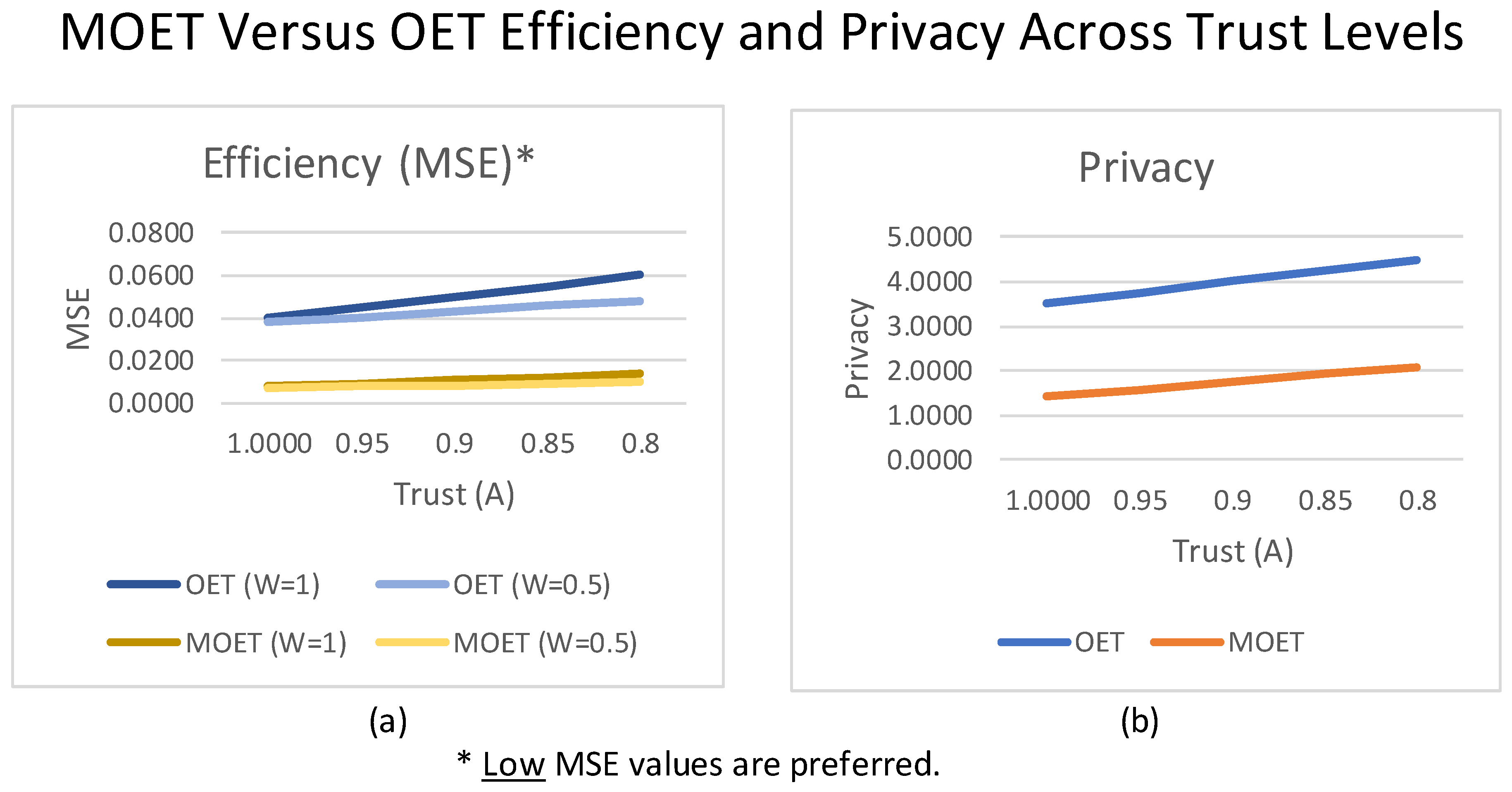
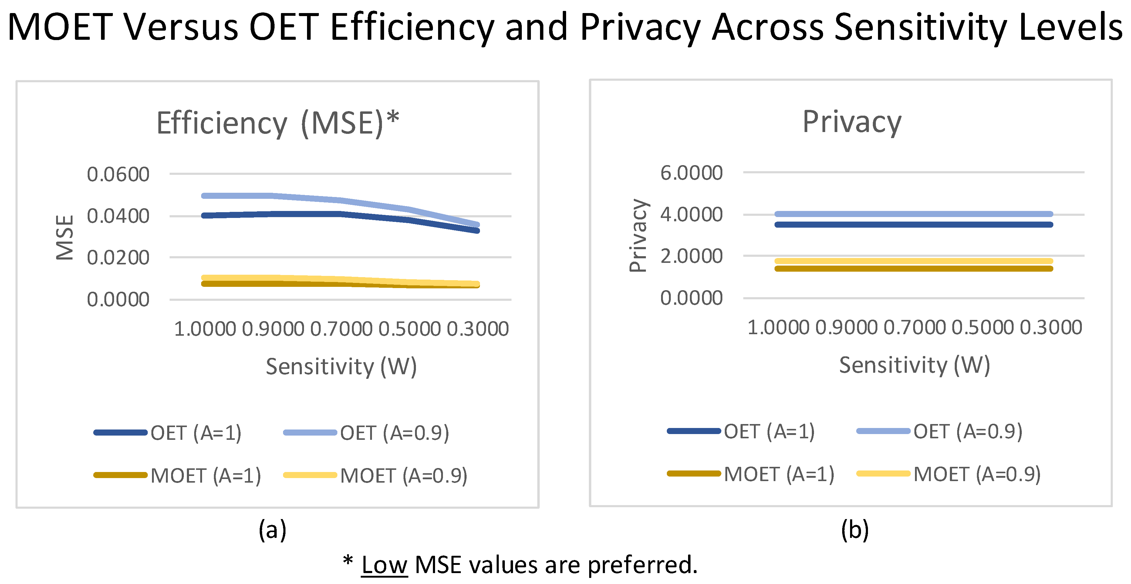
Recall that the two samples used to estimate ${\mathrm{\mu }}_Y$ yield the equations

$$E\left(Z_i\right)-{\mathrm{\mu }}_Y=W{\lambda }_i({\mathrm{\mu }}_R-{\mathrm{\mu }}_Y),\mathrm{i}=1,2.$$

(17)

Estimating ${E(Z}_i)$ by $\overline{Z_i}$ and ${\mathrm{\mu }}_Y$ by $\widehat{{\mathrm{\mu }}_Y}$, we have:

$$E(Z_i)-{\mathrm{\mu }}_Y=\widehat{W}{\lambda }_i({\mathrm{\mu }}_R-{\mathrm{\mu }}_Y),\mathrm{i}=1,2.$$

(18)

Solving the above expression for $W$ in samples 1 and 2 and then combining estimates, we have:

$$\widehat{W}=\frac{{\lambda }_2({\overline{Z}}_1-\widehat{{\mathrm{\mu }}_Y})+{\lambda }_1({\overline{Z}}_2-\widehat{{\mathrm{\mu }}_Y})}{2{{\lambda }_1\lambda }_2({\mathrm{\mu }}_R-\widehat{{\mathrm{\mu }}_Y})},{\lambda }_i=\left(1-\mathsf{\alpha }\right)\left(1-p_i\right),p_1\ne p_2.$$

(19)

Inserting our estimator for $\widehat{{\mathrm{\mu }}_Y}$, this expression reduces to

$$\widehat{W}=\frac{{\overline{Z}}_1-{\overline{Z}}_2}{{\lambda }_1\left({\mathrm{\mu }}_R-{\overline{Z}}_2\right)-{\lambda }_2({\mathrm{\mu }}_R-{\overline{Z}}_1)},{\lambda }_i=\left(1-\mathsf{\alpha }\right)\left(1-p_i\right),p_1\ne p_2.$$

(20)

From Equation (19) one can see that this estimator becomes unstable when ${\mathrm{\mu }}_R$ is close to ${\mathrm{\mu }}_Y.$

4. Discussion

In this section of the study, we provide two tables that represent theoretical and simulated values and illustrate important characteristics of the MOET model. Each row of each table represents the output from a particular scenario (combination of A, W, and α values). Each scenario represents a sampling of n = 500 respondents within an RRT sampling scenario, and each simulation sampling is conducted N = 10,000 times in R software.

Table 1. MOET Results. $(p_1=0.85,p_2=0.15,{\mu }_Y=2,{\mu }_S=0,{\mu }_T=1,{\mu }_R=2,{\sigma }_Y=1,{\sigma }_S=1,{\sigma }_T=1,{\sigma }_R=1,n=500,N=\mathrm{10,000}$).

A	W	α	${\widehat{\mathit{\mu }}}_{\mathit{Y}}$	${{\mathit{M}\mathit{S}\mathit{E}(\widehat{\mathit{\mu }}}_{\mathit{Y}})}_{\mathit{T}}$ *	${{\mathit{M}\mathit{S}\mathit{E}(\widehat{\mathit{\mu }}}_{\mathit{Y}})}_{\mathit{E}}$ *	${\left({𝛻}^{\mathit{a}}\right)}_{\mathit{T}}$ *	${\left({𝛻}^{\mathit{a}}\right)}_{\mathit{E}}$ *	${\left({\mathit{\delta }}^{\mathit{a}}\right)}_{\mathit{T}}$ *	${\left({\mathit{\delta }}^{\mathit{a}}\right)}_{\mathit{E}}$ *
1	1	1.0	2.0005	0.0122	0.0124	1.0000	1.0002	0.0122	0.0124
1	1	0.8	2.0017	0.0109	0.0111	1.0000	1.0003	0.0109	0.0111
1	1	0.6	2.0001	0.0097	0.0098	1.0000	0.9991	0.0097	0.0098
1	1	0.4	2.0021	0.0085	0.0083	1.0000	1.0012	0.0085	0.0083
1	1	0.2	1.9996	0.0073	0.0073	1.0000	1.0007	0.0073	0.0073
1	1	0	1.9999	0.0061	0.0061	1.0000	1.0016	0.0061	0.0061
1	0.6	1.0	2.0002	0.0097	0.0098	1.0000	1.0002	0.0097	0.0098
1	0.6	0.8	2.0005	0.0090	0.0092	1.0000	1.0003	0.0090	0.0092
1	0.6	0.6	2.0002	0.0083	0.0083	1.0000	0.9991	0.0083	0.0083
1	0.6	0.4	1.9999	0.0075	0.0075	1.0000	1.0012	0.0075	0.0075
1	0.6	0.2	1.9995	0.0068	0.0069	1.0000	1.0007	0.0068	0.0069
1	0.6	0	2.0006	0.0061	0.0062	1.0000	1.0016	0.0061	0.0062
1	0.2	1.0	1.9988	0.0073	0.0074	1.0000	1.0002	0.0073	0.0074
1	0.2	0.8	1.9988	0.0071	0.0069	1.0000	1.0003	0.0071	0.0069
1	0.2	0.6	2.0001	0.0068	0.0069	1.0000	0.9991	0.0068	0.0069
1	0.2	0.4	2.0006	0.0066	0.0066	1.0000	1.0012	0.0066	0.0066
1	0.2	0.2	2.0000	0.0063	0.0062	1.0000	1.0007	0.0063	0.0062
1	0.2	0	1.9996	0.0061	0.0062	1.0000	1.0016	0.0061	0.0062
0.9	1	1.0	2.0004	0.0152	0.0154	1.5000	1.5004	0.0101	0.0103
0.9	1	0.8	2.0002	0.0140	0.0137	1.4600	1.4585	0.0096	0.0094
0.9	1	0.6	1.9992	0.0128	0.0125	1.4200	1.4207	0.0090	0.0088
0.9	1	0.4	2.0016	0.0115	0.0116	1.3800	1.3798	0.0083	0.0084
0.9	1	0.2	1.9999	0.0103	0.0104	1.3400	1.3393	0.0077	0.0078
0.9	1	0	1.9992	0.0091	0.0089	1.3000	1.2982	0.0070	0.0069
0.9	0.6	1.0	2.0002	0.0116	0.0116	1.5000	1.5004	0.0077	0.0077
0.9	0.6	0.8	1.9992	0.0108	0.0109	1.4600	1.4585	0.0074	0.0075
0.9	0.6	0.6	1.9996	0.0101	0.0101	1.4200	1.4207	0.0071	0.0071
0.9	0.6	0.4	1.9988	0.0094	0.0092	1.3800	1.3798	0.0068	0.0067
0.9	0.6	0.2	2.0000	0.0086	0.0085	1.3400	1.3393	0.0064	0.0063
0.9	0.6	0	1.9995	0.0079	0.0080	1.3000	1.2982	0.0061	0.0062
0.9	0.2	1.0	2.0005	0.0079	0.0078	1.5000	1.5004	0.0053	0.0052
0.9	0.2	0.8	1.9989	0.0077	0.0076	1.4600	1.4585	0.0053	0.0052
0.9	0.2	0.6	2.0004	0.0074	0.0075	1.4200	1.4207	0.0052	0.0053
0.9	0.2	0.4	2.0001	0.0072	0.0072	1.3800	1.3798	0.0052	0.0052
0.9	0.2	0.2	2.0022	0.0069	0.0070	1.3400	1.3393	0.0051	0.0052
0.9	0.2	0	2.0007	0.0067	0.0069	1.3000	1.2982	0.0052	0.0053

* ${{MSE(\widehat{\mathrm{\mu }}}_Y)}_T$ and ${{MSE(\widehat{\mathrm{\mu }}}_Y)}_E$ represent theoretical and empirical mean squared error of the estimator of $Y$. ${\left({𝛻}^a\right)}_T$ and ${\left({𝛻}^a\right)}_E$ represent theoretical and empirical model privacy. ${\left({\delta }^a\right)}_T$ and ${\left({\delta }^a\right)}_E$ represent theoretical and empirical unified measure.

shows that the estimators developed in this study perform in line with theoretical expectations. Table 1 also establishes the value of the mixture model by showing that the MOET model—which is fundamentally a mixture of a Greenberg-based and a Warner-based model—yields performance preferable to either model on its own.

Table 2. MOET Results compared to OET Results. $(\alpha {=0.15,p}_1=0.85,p_2=0.15,{\mu }_Y=2,{\mu }_S=0,{\mu }_{S1}=2,{\mu }_{S2}=1,{\mu }_T=1,{\mu }_R=1,{\sigma }_Y=1,{\sigma }_S=1,{\sigma }_T=1,{\sigma }_R=1,n=500,N=\mathrm{10,000}$).

			OET Model						MOET Model
A	W		${\widehat{\mathit{\mu }}}_{\mathit{Y}}$	${{\mathit{M}\mathit{S}\mathit{E}(\widehat{\mathit{\mu }}}_{\mathit{Y}})}_{\mathit{T}}$	${\left({𝛻}^{\mathit{a}}\right)}_{\mathit{T}}$ *	${\left({\mathit{\delta }}^{\mathit{a}}\right)}_{\mathit{T}}$	$\widehat{\mathit{W}}$		${\widehat{\mathit{\mu }}}_{\mathit{Y}}$	${{\mathit{M}\mathit{S}\mathit{E}(\widehat{\mathit{\mu }}}_{\mathit{Y}})}_{\mathit{T}}$	${\left({𝛻}^{\mathit{a}}\right)}_{\mathit{T}}$	${\left({\mathit{\delta }}^{\mathit{a}}\right)}_{\mathit{T}}$	$\widehat{\mathit{W}}$
1	1		1.99899	0.0400	3.500	0.0114	1.0001		2.00122	0.0077	1.4250	0.0054	0.9956
1	0.9		2.0017	0.0409	3.500	0.0117	0.8989		1.9996	0.0075	1.4250	0.0053	0.8938
1	0.7		1.9975	0.0407	3.500	0.0116	0.7023		1.9993	0.0072	1.4250	0.0051	0.6938
1	0.5		1.9985	0.0380	3.500	0.0109	0.5013		2.0010	0.0069	1.4250	0.0048	0.4941
1	0.3		1.9999	0.0327	3.500	0.0093	0.3001		1.9997	0.0066	1.4250	0.0046	0.2914
0.95	1		2.0014	0.0450	3.750	0.0120	0.9989		1.9994	0.0092	1.5900	0.0058	0.9953
0.95	0.9		1.9991	0.0454	3.750	0.0121	0.9014		1.9990	0.0089	1.5900	0.0056	0.8933
0.95	0.7		2.0024	0.0442	3.750	0.0118	0.6980		2.0010	0.0083	1.5900	0.0052	0.6933
0.95	0.5		2.0006	0.0405	3.750	0.0108	0.4996		2.0005	0.0077	1.5900	0.0048	0.4925
0.95	0.3		1.9966	0.0342	3.750	0.0091	0.3030		1.9999	0.0071	1.5900	0.0045	0.2901
0.9	1		2.0010	0.0500	4.000	0.0125	0.9993		2.0007	0.0107	1.7550	0.0061	0.9960
0.9	0.9		1.9997	0.0499	4.000	0.0125	0.9000		1.9995	0.0103	1.7550	0.0059	0.8925
0.9	0.7		2.0010	0.0477	4.000	0.0119	0.6997		1.9996	0.0094	1.7550	0.0054	0.6916
0.9	0.5		1.9988	0.0430	4.000	0.0108	0.5013		1.9975	0.0084	1.7550	0.0048	0.4883
0.9	0.3		2.0000	0.0357	4.000	0.0089	0.3012		2.0002	0.0075	1.7550	0.0043	0.2889
0.85	1		2.0038	0.0550	4.250	0.0129	0.9980		2.0017	0.0122	1.9200	0.0064	0.9936
0.85	0.9		2.0024	0.0544	4.250	0.0128	0.8984		1.9996	0.0116	1.9200	0.0060	0.8910
0.85	0.7		2.0032	0.0512	4.250	0.0120	0.6988		1.9995	0.0104	1.9200	0.0054	0.6915
0.85	0.5		2.0002	0.0455	4.250	0.0107	0.4997		2.0000	0.0092	1.9200	0.0048	0.4882
0.85	0.3		1.9996	0.0372	4.250	0.0088	0.3000		2.0001	0.0080	1.9200	0.0042	0.2908
0.8	1		2.0028	0.0600	4.500	0.0133	0.9987		1.9974	0.0137	2.0850	0.0066	0.9917
0.8	0.9		2.0036	0.0589	4.500	0.0131	0.8982		2.0005	0.0130	2.0850	0.0062	0.8915
0.8	0.7		1.9997	0.0547	4.500	0.0122	0.7004		1.9996	0.0115	2.0850	0.0055	0.6895
0.8	0.5		2.0041	0.0480	4.500	0.0107	0.4971		2.0010	0.0100	2.0850	0.0048	0.4906
0.8	0.3		1.9990	0.0387	4.500	0.0086	0.3008		2.0000	0.0084	2.0850	0.0040	0.28888

* ${{MSE(\widehat{\mathrm{\mu }}}_Y)}_T$, ${\left({𝛻}^a\right)}_T$, and ${\left({\delta }^a\right)}_T$ represent the theoretical mean squared error, privacy and unified measure for the respective models. Green indicates model superiority.

compares MOET model statistics to published OET model statistics in Gupta et al. (2022), and thereby demonstrates the MSE and unified measure superiority of the MOET model to the OET model [6].

Table 1 shows the results from the MOET model run according to the parameter values listed. The close fit between the empirical and theoretical values speaks to the veracity of the formulae proposed in this study, as well as the accuracy of the empirical simulations.

We draw attention to three particularly important aspects of the scenario presented in Table 1. First, observe that in the shown scenario, maximum efficiency (minimum MSE) occurs when α = 0 for any pairing of $A$ and $W$ values. Mathematically, this does not have to be true in every scenario. For example, in the scenario underlying the table above, the extreme choice of ${\mathsf{\sigma }}_R^2=7$ with all other assumptions left unchanged will lead to a circumstance where maximum efficiency is found at α = 1 rather than α = 0. To study this important relationship closely, we let $f\left(a\right)=Var\left(\widehat{{\mu }_Y}\right)$, per Equation (13), and then take the derivative of this expression with respect to $a$. Expressing the result in the form below, we can see that $f\prime \left(a\right)$ will always be positive under certain conditions.

$$f^{\prime }\left(a\right)={\left(\frac{1-p_1}{p_2-p_1}\right)}^2\frac{2}{n}\left[{\psi }_2+{\mathsf{{\rm X}}}_2+{\mathsf{{\rm Y}}}_2+{\mathsf{\zeta }}_2\right]+{\left(\frac{1-p_2}{p_2-p_1}\right)}^2\frac{2}{n}\left[{\psi }_1+{\mathsf{{\rm X}}}_1+{\mathsf{{\rm Y}}}_1+{\mathsf{\zeta }}_1\right],$$

(21)

$${\psi }_i={\mathrm{A}\mathrm{W}{p}_i\mathsf{\sigma }}_S^2,$$

$${\mathsf{{\rm X}}}_i=\left(1-p_i\right)W({\left(\left(1-A\right){\mathsf{\sigma }}_T^2+1\right)\left({\mathsf{\sigma }}_Y^2+{\mu }_Y^2\right)+\mathsf{\sigma }}_S^2-{\mathsf{\sigma }}_R^2-{\mu }_R^2),$$

$${\mathsf{{\rm Y}}}_i=2\left({\mu }_R-{\mu }_Y\right)W\left(1-p_i\right){\mu }_Y,$$

$${\mathsf{\zeta }}_i=2{(1-a)\left({\mu }_R-{\mu }_Y\right)}^2{W}^2{\left(1-p_i\right)}^2,$$

$$i=1,2.$$

Specifically, under the following two sufficient but not necessary conditions, $f\prime \left(a\right)$ will be positive across all $a$ values, so $Var\left(\widehat{{\mu }_Y}\right)$ will be an increasing function of $a$. That is, maximum efficiency (minimum MSE) will always occur when α = 0 if

$${\mu }_R={\mu }_Y,$$

(22a)

$$\left(\left(1-A\right){\mathsf{\sigma }}_T^2+1\right)\left({\mathsf{\sigma }}_Y^2+{\mu }_Y^2\right)+{\mathsf{\sigma }}_S^2>{\mathsf{\sigma }}_R^2+{\mu }_R^2.$$

(22b)

The first condition sets ${\mathrm{\mu }}_R$ equal to ${\mathrm{\mu }}_Y$, which seems both reasonable and intuitively appealing, as the response to the unrelated question should be designed to have a similar size to that of the sensitive question under study. Because the first condition fixes ${\mathrm{\mu }}_R$, the second condition puts an upper limit on the size of ${\mathsf{\sigma }}_R^2$. This is not a very restrictive condition. Note that with A = 1, condition (22b) for the scenario presented in Table 1 reduces to ${\mathsf{\sigma }}_R^2<2$. Our choice of ${\mathsf{\sigma }}_R^2=1$ meets the condition comfortably.

The second important aspect of Table 1 is that it illustrates the importance of the mixture feature of the model. The mixture capability of MOET is necessary to strike an optimal balance between the model’s efficiency and its privacy. This is clear because maximum efficiency is typically achieved when α is low (mixture leans toward the Greenberg model), while maximum privacy is achieved when α is high (mixture leans toward the Warner model), providing A < 1. For example, when $A$ = 0.9 and $W=1$, theoretical privacy improves from 1.3 to 1.5 as α values increase from 0 to 1, but at the same time that privacy improves, efficiency declines (MSE increases from 0.0091 to 0.0152). Since RRT models must achieve strong levels of both privacy and efficiency, the choice of an α value of 0 or 1 (full Greenberg or full Warner) would be a poor choice; they would either sacrifice the model’s privacy to maximize its efficiency or vice versa. A choice of α between 0 and 1 (some mixture) will better balance the competing concerns.

Beyond the two key observations made above, Table 1 also confirms that the model behaves in many expected ways. When question sensitivity ($W$) is low, the model is more efficient. For example, when A = 1 and α = 0.6, efficiency is higher (MSE lower) for W = 0.2 (0.0069) than for W = 1 (0098). This relationship is intuitive because more respondents submit their responses without any RRT scrambling when W = 0.2, leading to greater efficiency.

When respondents do not require additional scrambling to enhance their trust (when $A$ is large), the model is more efficient. For example, when W = 0.6 and α = 0.6, efficiency is higher (MSE lower) for A = 1 (0.0083) than for W = 0.9 (0101). Again, this result seems intuitively reasonable. Note that Table 1 was run with ${\mathrm{p}}_1=0.15$ and ${\mathrm{p}}_2=0.85$. These values were chosen because widely disparate probability values lead to higher model efficiency (this is a known characteristic of the split sample approach).

The exact nature of the tradeoff between efficiency and privacy across α values, and in fact the existence of any tradeoff at all, is influenced by the sensitivity of the particular quantitative research question ($W$) and the respondent’s need for enhanced trust ($A$), as well as by the standard deviations of the chosen scrambling variables, $S$ and $T$, and the mean and variance of the unrelated question response $R$. We make this observation as a way of drawing attention to the high level of flexibility in the model. For a given quantitative research scenario in which a researcher has specific efficiency and privacy goals, the researcher can strategically choose the MOET model’s $S$, $T$ and $R$ variables and the mixture split α that will most closely achieve those goals.

Table 2 is provided principally to facilitate comparisons between the MOET model and its predecessor, the OET model (see Appendix A). The OET model, in fact, can be thought of as a special case of the MOET model with α = 1. Comparison of Equation (A1) to Equation (9) makes this relationship clear.

Recall that we have established, based on Table 1, that the empirical values of each of these statistics falls close to their theoretical values, so for purposes of legibility, the empirical values of these quantities are not shown here. The scenarios run for the OET and MOET models represented in Table 2 are the same, and the values of all parameters equal the values used in the published Gupta et al. (2022) OET model paper [6]. That is, the values of all parameters that the two models have in common (${\mathsf{\sigma }}_{\mathrm{S}}$, ${\mathrm{\mu }}_{\mathrm{T}}$, ${\mathsf{\sigma }}_{\mathrm{T}})$, the assumed characteristics of the sensitive question (${\mathrm{\mu }}_{\mathrm{Y}}$, ${\mathsf{\sigma }}_{\mathrm{Y}},$ $W$), the inclination of the respondent to respond without additional scrambling ($A$), the sample size, and number of iterations run (n, N), are the same in both models.

For the table above, we have set ${\mathrm{\mu }}_{\mathrm{R}}$ = 1 rather than ${{\mathrm{\mu }}_{\mathrm{R}}=\mathrm{\mu }}_{\mathrm{Y}}=2$. This choice was made because the estimator for $W$ (see Equation (19)) becomes volatile when ${{\mathrm{\mu }}_{\mathrm{R}}=\mathrm{\mu }}_{\mathrm{Y}}$. The choice of ${\mathrm{\mu }}_{\mathrm{R}}$ = 1 caused privacy to improve but caused efficiency to deteriorate slightly. In a real-life scenario, a researcher could choose ${\mathrm{\mu }}_{\mathrm{R}}$ to accommodate their research needs, choosing ${\mathrm{\mu }}_{\mathrm{R}}$ far from ${\mathrm{\mu }}_{\mathrm{Y}}$ if an estimate of W is needed.

The Table 2 scenario shows the MOET model’s efficiency to be superior to that of the OET model. For example, in the circled row, when A = 0.95 and W = 0.9, we can see that (MSE = 0.0089) < (MSE = 0.0454), implying that the MOET has superior efficiency; this efficiency superiority in fact holds true for all A and W values in the table. It follows that in scenarios where efficiency is significantly more important than privacy, the MOET model will often be the better choice of model. However, the OET model outperforms the MOET in terms of privacy. See Figure 2 and Figure 3 below that illustrate the tabular data above:

While in the illustrated scenario MOET outperforms OET in terms of efficiency, OET outperforms MOET in terms of privacy. When we combine the two measures, we see that the MOET model outperforms the OET model according to the unified measure. For example, when A = 1 and W = 1, we can see in Table 2 that (${\delta }^a$ = 0.0056) < (${\delta }^a$ = 0.0121); the superiority of the MOET model in terms of unified measure holds true for all A and W values.

5. Conclusions

The Mixture-Optional Enhanced Trust model proposed in this study has important advantages over the OET model, which in turn was shown to be superior to the basic Warner model (Gupta et al. 2022) [6]. Specifically, the MOET model can yield lower MSE (therefore higher efficiency) than the OET model when MOET parameters are elected that favor efficiency over privacy. But the OET model generally achieves superior privacy, so it will usually be the better model in cases where the need for privacy is the overriding concern. This lower MSE of the MOET model offsets the higher privacy offered by the OET model, as indicated by superior unified measure values. In this study, we have shown, furthermore, that the MOET model’s mixture capability (captured by model parameter α) causes MOET to be superior to either a full Warner-based or a full Greenberg-based model. This mixture model will balance the competing concerns of privacy and efficiency, which will always be preferable to fully sacrificing one of these important characteristics for the other.

References

1. Raghavarao, D.; Federer, W.T. Block total response as an alternative to the randomized response method in surveys. J. R. Stat. Soc. Ser. B (Methodol.) 1979, 41, 40–45. [Google Scholar] [CrossRef]
2. Reynolds, W. Development of a reliable and valid short form of the Marlowe-Crowne SDB scale. J. Clin. Psychol. 1982, 38, 119–125. [Google Scholar] [CrossRef]
3. Jones, E.; Sigall, H. The Bogus Pipeline: A new paradigm for measuring effect and attitude. Psychol. Bull. 1971, 76, 349–364. [Google Scholar] [CrossRef]
4. Warner, S. The Linear Randomized Response Model. J. Am. Stat. Assoc. 1971, 66, 884–888. [Google Scholar] [CrossRef]
5. Greenberg, B.G.; Abul-Ela, A.L.A.; Simmons, W.R.; Horvitz, D.G. The unrelated question randomized response model: Theoretical framework. J. Am. Stat. Assoc. 1971, 666, 243–250. [Google Scholar] [CrossRef]
6. Gupta, S.; Zhang, J.; Khalil, S.; Sapra, P. Mitigating Lack of Trust in Quantitative Randomized Response Techniques Models. Commun. Stat. Part B Simul. Comput. 2022, 51, 1–9. [Google Scholar] [CrossRef]
7. Mehta, S.; Aggarwal, P. Bayesian estimation of sensitivity level and population proportion of a sensitive characteristic in a binary optional unrelated question rrt model. Commun. Stat.—Theory Methods 2018, 47, 4021–4028. [Google Scholar] [CrossRef]
8. Diana, G.; Perri, P.F. A class of estimators for quantitative sensitive data. Stat. Pap. 2011, 52, 633–650. [Google Scholar] [CrossRef]
9. Singh, G.N.; Kumar, A.; Vishwakarma, G.K. Some alternative additive randomized response models for estimation of population mean of quantitative sensitive variable in the presence of scramble variable. Commun. Stat.-Simul. Comput. 2018, 49, 2785–2807. [Google Scholar] [CrossRef]
10. Priyanka, K.; Trisandhya, P. A composite class of estimators using scrambled response mechanism for sensitive population mean in successive sampling. Commun. Stat.—Theory Methods 2019, 48, 1009–1032. [Google Scholar] [CrossRef]
11. Gupta, S.; Gupta, B.; Singh, S. Estimation of the sensitivity level of personal interview survey questions. J. Stat. Plan. Inference 2002, 100, 239–247. [Google Scholar] [CrossRef]
12. Gupta, S.; Mehta, S.; Shabbir, J.; Khalil, S. A unified measure of respondent privacy and model efficiency in quantitative RRT models. J. Stat. Theory Pract. 2018, 12, 506–511. [Google Scholar] [CrossRef]
13. Vishwakarma, G.K.; Kumar, A.; Kumar, N. Two-stage unrelated randomized response model to estimate the prevalence of a sensitive attribute. Comput. Stat. 2023, 52, 1–26. [Google Scholar] [CrossRef]
14. Narjis, G.; Shabbir, J. An efficient partial randomized response model for estimating a rare sensitive attribute using poisson distribution. Commun. Stat.—Theory Methods 2021, 50, 1–17. [Google Scholar] [CrossRef]
15. Lovig, M.; Khalil, S.; Rahman, S.; Sapra, P. A mixture binary RRT model with a unified measure of privacy and efficiency. Commun. Stat.—Simul. Comput. 2021, 52, 2727–2737. [Google Scholar] [CrossRef]
16. Yan, Z.; Wang, J.; Lai, J. An Efficiency and Protection Degree-Based Comparison Among the Quantitative Randomized Response Strategies. Theory Methods 2008, 38, 400–408. [Google Scholar] [CrossRef]
Figure 1. MOET model.
Axioms 13 00011 g001
Figure 2. MOET vs. OET comparison across trust levels. (a) Efficiency results for MOET and OET models across trust levels (A). (b) Privacy results for MOET and OET models across trust levels (A). Parameter values underlying these exhibits are those cited in Table 2.
Axioms 13 00011 g002
Figure 3. MOET vs. OET comparison across sensitivity levels. (a) Efficiency results for MOET and OET models across sensitivity levels (W). (b) Privacy results for MOET and OET models across sensitivity levels (W). Parameter values underlying these exhibits are those cited in Table 2.
Axioms 13 00011 g003