Abstract
With the widespread application of spatial data in fields like econometrics and geographic information science, the methods to enhance the robustness of spatial econometric model estimation and variable selection have become a central focus of research. In the context of the spatial error model (SEM), this paper introduces a variable selection method based on exponential square loss and the adaptive lasso penalty. Due to the non-convex and non-differentiable nature of this proposed method, convex programming is not applicable for its solution. We develop a block coordinate descent algorithm, decompose the exponential square component into the difference of two convex functions, and utilize the CCCP algorithm in combination with parabolic interpolation for optimizing problem-solving. Numerical simulations demonstrate that neglecting the spatial effects of error terms can lead to reduced accuracy in selecting zero coefficients in SEM. The proposed method demonstrates robustness even when noise is present in the observed values and when the spatial weights matrix is inaccurate. Finally, we apply the model to the Boston housing dataset.
MSC:
62F12; 62G08; 62G20; 62J07
1. Introduction
With the widespread application of spatial effects data in various fields such as spatial econometrics, geography, and epidemiology, spatial regression models used for handling such data have been extensively studied by many scholars. Spatial effects include spatial correlation (dependence) and spatial heterogeneity. To reflect different forms of spatial correlation, Anselin (1988) [1] categorized spatial econometric models into spatial autoregressive models (SARs), spatial Durbin models (SDMs), and spatial error models (SEMs). Among them, the spatial error model is represented as . The spatial error model (SEM) considers the mutual influence between spatially adjacent regions. The fundamental idea is to incorporate spatial autocorrelation as an error term into the regression model, addressing the limitation of traditional regression models in handling spatial autocorrelation issues. In the SEM model, the error terms are no longer independently and identically distributed but exhibit spatial autocorrelation with the error terms of neighboring regions.
With the rapid increase in data dimensionality, the issue of variable selection in spatial error models has attracted widespread attention. In the classic field of linear regression, there have been numerous studies on variable selection. Penalty methods are commonly used for model variable selection, and several penalty functions have been proposed, such as the least absolute shrinkage and selection operator (LASSO, Tibshirani, 1996 [2]), smoothed trimmed absolute deviation (SCAD, Fan and Li, 2001 [3]) and adaptive lasso (Zou, 2006 [4]). Due to the spatial dependence inherent in SEM, the aforementioned penalty methods can be directly applied to variable selection in the spatial error model.
Due to observation noise and inaccurate spatial weight matrices, traditional variable selection methods can become unstable and inaccurate in parameter estimation. This can also lead to misguidance in variable selection, resulting in the erroneous choice of variables that do not reflect the actual situation.Therefore, efforts have been made to adopt more robust approaches. Many studies employ the Huber loss function (Huber, 2004 [5]); however, the Huber loss function may not be sufficiently robust in the presence of extreme outliers, and it often leads to high computational complexity when dealing with high-dimensional data. Wang et al. (2013) [6] introduced a class of robust estimates with exponential square loss functions . For large values of , the exponential square estimates are similar to the least squares estimates; when is very small, larger absolute values of observations will result in an empirical loss close to 1.0. Therefore, outliers have little impact on the estimates when is small, limiting the influence of outliers on the estimates. In contrast, this method exhibits stronger robustness compared to other robust methods, including Huber estimates (Huber, 2004 [5]), quantile regression estimates (Koenker and Bassett, 1978 [7]), and composite quantile regression estimates (Zou and Yuan, 2008 [8]). Wang et al. (2013) [6] also introduced a method for selecting the parameter .
We focus on the variable selection problem of the spatial error model (SEM). However, currently, there is not much exploration regarding robust variable selection methods for spatial error models. Liu et al. (2020) [9] employed penalized pseudo-likelihood and SCAD penalties for variable selection in the spatial error model. Through Monte Carlo simulations, they demonstrated that this method exhibits good variable selection performance based on normal data. Dogan (2023) [10] used modified harmonic mean estimates to estimate the marginal likelihood function of the cross-sectional spatial error model, thereby improving the estimation performance of spatial error model parameters. However, their methods are still susceptible to the influence of outliers. Therefore, exploring more robust variable selection methods is imperative. Considering the robustness of the exponential square loss function, we employ an adaptive lasso penalty method in conjunction with the exponential square loss to penalize all unknown parameters in the loss function except for the variance of the random disturbance term. Song et al. (2021) [11] applied this method to the SAR model and achieved satisfactory results. In this paper, we apply the same method to the SEM model. We construct the following optimization model:
where , , and are all parameters to be estimated, and , . is a non-negative regularization term weight coefficient. is a penalty term, and is the exponential square loss mentioned earlier.
Due to the non-convex nature of the exponential square loss function, the empirical loss term is inherently a structured non-convex function with respect to three variable blocks, namely . Furthermore, since many penalty methods (lasso or adaptive lasso) are non-differentiable, (1) represents a non-convex, non-differentiable optimization problem. In this paper, we propose a robust variable selection method for the spatial error model based on the exponential squared loss function and adaptive lasso penalty. This method allows for the selection of variables while simultaneously estimating the regression coefficients. The main contributions of this paper are as follows.
- (1)
- We established a robust variable selection method for SEM, which employs the exponential squared loss and demonstrates good robustness in the presence of outliers in the observations and inaccurate estimation of the spatial weight matrix.
- (2)
- We designed a BCD algorithm to solve the optimization problem in SEM. We decomposed the exponential square loss component into the difference of convex functions and built a CCCP program for solving the BCD algorithm subproblems. We utilized an accelerated FISTA algorithm to solve the optimization problem with the adaptive lasso penalty term. We also provide the computational complexity of the BCD algorithm.
- (3)
- We verified the robustness and effectiveness of this method through numerical simulation experiments. The simulation results indicate that neglecting the spatial effects of error terms leads to a decrease in variable selection accuracy. When there is noise in the observations and inaccuracies in the spatial weight matrix, the method proposed in this paper outperforms the comparison methods in correctly identifying zero coefficients, non-zero coefficients, and median squared error (MedSE).
The organizational structure of this paper is as follows: In Section 2, we introduce the SEM model, construct the loss function with exponential squared loss and adaptive lasso regularization, and provide methods for selecting model hyperparameters and estimating variance. In Section 3, we design an efficient algorithm to optimize the loss function, accomplishing variable selection and parameter estimation. Section 4 includes numerical simulation experiments to assess the variable selection and estimation performance of the proposed method. In Section 5, we apply this method to the Boston Housing dataset. Finally, in Section 6, we summarize the entire paper.
2. Model Estimation and Variable Selection
2.1. Spatial Error Model
We consider the following SEM model with covariates
where , is an n-dimensional response vector, is the design matrix, and is the error vector. W and M are spatial weight matrix. In practical applications, M is often constructed using a spatial rook matrix. The spatial autocorrelation coefficients and are scalars, while measures the impact of errors in the dependent variable in neighboring areas on the local observations. A larger indicates a stronger spatial dependence effect in the sample observations, while a smaller implies a weaker effect. A high-order spatial error model with p lag terms and q disturbance terms is typically represented as follows:
This study considers a first-order spatial error model. is an n-dimensional identity matrix. It is typically assumed that is independently and identically distributed, i.e., . Therefore, U and Y can be represented as follows:
where it is necessary to ensure that and are invertible. According to Banerjee et al. (2014) [12], under certain normalization operations, the maximum singular value of the matrix W is 1. Therefore, condition ensures the invertibility of (). We impose constraints on and , i.e., and . Furthermore, we neglect the endogeneity induced by spatial dependence (Ma et al., 2020) [13].
2.2. Variable Selection Methods
This section considers variable selection for model (2). Following Fan and Li (2001) [3], it is typically assumed that the regression coefficient vector is sparse. A natural approach is to use penalty methods for model handling, which can simultaneously select important variables and estimate unknown parameters. The constructed penalty method can be represented as follows:
When considering the choice of penalty methods, this paper opts for the adaptive lasso penalty. Let be a consistent estimator of . Following the recommendation of Zou (2006) [4], we set and define the weight vector . The adaptive lasso is redefined as
The penalty-robust regression formula with an exponential square loss and adaptive lasso penalty is redefined as
where , , and is the exponential square loss mentioned earlier . is a positive regularization coefficient. The selection of the tuning parameter in the exponential square function will be discussed in the next section.
2.3. The Selection of
The parameter controls the robustness and estimation efficiency of the proposed variable selection method. Wang et al. (2013) [6] introduced a method for selecting . It first identifies a set of tuning parameters such that the proposed penalty estimates have an asymptotic break-even point at 0.5, and then selects the parameter based on the principle of maximum efficiency. The process is as follows:
Step 1. Initialize a set of parameters with , , , where . Rewrite the model as , where and .
Step 2. Let be a sample set that consists of a collection of samples, and calculate and . Then, there exists a set of pseudo-outliers
, , and .
Step 3. Construct , where
Next, let be the minimum value of in the set , where is defined the same way as in Wang et al. (2013) [6].
Step 4. The optimal solution from the optimization problem updates , , and , where and . Terminate if the result converges; otherwise, return to Step 2.
Considering the potential difficulties arising from the significant computational burden, we do not use cross validation to select and the penalty coefficient . In practical applications, we can find a threshold for which . The values of typically fall within the interval . In the initial steps mentioned above, an initial estimate is required. In numerical simulations, we use an estimate with the LAD loss as the initial estimate.
2.4. The Selection of and
When considering the selection of and , it is common to unify the two parameters: . Various methods such as AIC (Akaike Information Criterion), BIC (Bayesian Information Criterion), and cross validation can be used to choose these parameters.
To ensure the consistency of the variable selection and reduce computational complexity, we follow the method described in Wang et al. (2007) [14] by selecting the regularization parameter through the minimization of the BIC objective function. The objective function is as follows:
From this, we can deduce that . In practical applications, we may not know the values of , but we can easily obtain through the exponential square loss. In Section 2.3, we obtained the estimate for . It is important to note that when making this simple selection, the following conditions should be satisfied: and , where is the number of non-zero values in . This ensures the consistency of the variable selection in the final estimate.
2.5. Estimation of Noise Variance
We estimate the variance of the random disturbance term; let , , then the estimated variance of the random disturbance term V is given by
where , , and can be obtained by solving Equation (8). It is known from the constraints on and that both G and F are non-singular matrices. Let and . Then, the estimated defined in Equation (10) can be calculated using the following equation:
3. Model Solving Algorithm
This section outlines the algorithm for solving Equation (8). In this optimization problem, the objective function can be divided into three variable blocks: , , and . We can use a block coordinate descent algorithm to solve it. However, the objective function in Equation (8) is non-convex and non-smooth. Using block coordinate descent alone can be challenging to ensure convergence. Therefore, we perform a convex–concave procedure (CCCP) by decomposing the exponential square loss part and utilize the CCCP algorithm to solve the subproblem for . For the lasso and adaptive lasso penalty terms, we use the ISTA (Iterative Soft Thresholding) algorithm, and this paper employs an accelerated FISTA algorithm.
3.1. Block Coordinate Descent Algorithm
In Algorithm 1, we provide the framework of a block coordinate descent algorithm for the alternating iterative solution of .
The next tasks are to solve subproblems (14)–(16). Subproblems (14) and (15) can be transformed into single-variable function optimization problems with the other two parameters fixed. The range for achieving the optimal solution of the objective function is [0, 1]. Therefore, the parabolic interpolation-based golden section method can be employed for solving them. For specific algorithm details, please refer to Forsythe et al. (1977) [15]. In the next section, we will discuss the solution to (16) in detail.
| Algorithm 1 BCD algorithm framework. |
| 1. Set the initial iteration point , , ; 2. Repeat ; 3. Solve the subproblem about with initial point ; 4. Solve the subproblem about with initial point ; 5. Solve the subproblem with initial value , to obtain a solution , ensuring that , and that is a stationary point of . 6. Iterate until convergence. |
3.2. Solving Subproblem (16)
Given that the optimization problem is composed of the exponential square loss term and the lasso or adaptive lasso penalty term, it can be observed that when and are fixed, the lasso or adaptive lasso is convex. The exponential square loss can be decomposed into the difference of two convex functions. Therefore, subproblem (16) is a DC (difference of convex) program, and it can be solved using the appropriate algorithms. When decomposing the exponential square loss function into a DC form, we made the following attempts.
Proposition 1.
, We assume that , where both and are convex functions. We can assume that based on the non-negativity of the second derivative. Then, we set:
It can be proven that both and are convex functions, completing the DC decomposition of the exponential square part . We can then define the following two functions:
where and are defined in (17) and (18), and represent the i-th row of the spatial weight matrices W and M, is the convex penalty with respect to . Then, and are convex and concave functions, respectively. Subproblem (16) can be rewritten as
For this convex–concave procedure, we can use Algorithm 2 for solving it as described in Yuille et al. (2003) [16].
| Algorithm 2 Convex–concave procedure algorithm. |
| 1. Set an initial point and initialize . 2. Repeat 3. 4. Update the iteration counter: 5. Until convergence of |
The CCCP algorithm is a monotonically decreasing global optimization method that approximates the global optimal solution by alternating between optimizing the convex and concave parts. Therefore, it is possible to use iterative solutions to minimize the objective function in (21) by solving (22). We are considering which algorithm to use for solving (22) to improve the efficiency of Algorithm 2.
We notice that the first term in (22) consists of a convex function and a convex penalty term on given by , while the second term is a linear function of . We can rewrite (22) as follows:
where is a continuously differentiable convex function, defined as . Beck and Teboulle (2009) [17] introduced an algorithm called ISTA (Iterative Soft Thresholding Algorithm) to solve optimization problems with lasso penalties. Song et al. (2021) [11] proved that this algorithm can be applied to models with adaptive lasso penalties. Therefore, ISTA can be used to solve problems structured like (23). This paper chooses the accelerated version of ISTA, known as the FISTA algorithm, for optimization. The convergence properties of FISTA have been established by Beck and Teboulle (2009) [17]. Algorithm 3 provides an overview of the FISTA algorithm.
With this, we complete the algorithm design for solving (16). In addition, we provide the computational complexity of the BCD program and an introduction to the machine specifications used in subsequent experiments in Appendix B.
| Algorithm 3 FISTA algorithm with backtracking step for solving (22). |
|
Require: Ensure: solution 1: Step 0. Select . Let 2: Step . 3: Determine the smallest non-negative integer which makes satisfy 4: 5: Let and calculate: 6: 7: 8: 9: Output . |
4. Numerical Simulations
In this section, we conducted several sets of numerical simulations to validate the impact of spatial errors on the estimation and variable selection of the SEM model. We also compared the performance of the proposed variable selection method with other methods in various scenarios, including small and large sample sizes, the presence of many non-significant covariates, noisy response variable observations, and inaccurate spatial weight matrix.
4.1. Generation of Simulated Data
The data generation process is based on model (2). We consider covariates to follow a normal distribution with a mean of zero and a covariance matrix of , where . In other words, the design matrix is an matrix. Let the sample size and the number of non-significant covariates .
The spatial autoregressive coefficient follows a uniform distribution on the interval , where . To verify whether spatial dependence among response variables affects the model estimation and variable selection, an additional experiment with is included. In this case, the SEM model reduces to a linear error model. The spatial dependence coefficient in the error term is used to examine the influence of spatial effects in the error terms on SEM model estimation and variable selection. The coefficients for covariates are set as a sparse vector , where q is the number of non-significant covariates. The values of are sampled from a normal distribution with means of and a variance of , where is the identity matrix in .
Let the spatial weight matrix , where , ⊗ denotes the Kronecker product, and is an m-dimensional column vector consisting of ones. In this study, let . The error term’s spatial weight matrix M is constructed as a spatial rook matrix, considering only adjacent elements in the horizontal and vertical directions. In this matrix, adjacent element positions are set to 1, while all other positions are set to 0. The response variable Y and the error term U are generated according to the (4) and (5) provided in the context.
Independent random disturbance terms . The parameter is uniformly distributed in the interval [− 0.1, + 0.1], where . When considering noise in the response variables, the interference term follows a mixture of normal distributions. Specifically, V is distributed as a mixture of two normal distributions , where .
We also designed inaccurate spatial weight matrix W by randomly removing of the non-zero values in each row of W and adding non-zero elements randomly in each row of W. Then, the constructed inaccurate W was normalized and used in the SEM model.
Each scenario was based on 100 simulations. To gauge the model’s superiority, we compared it with square loss and absolute loss. For accurate performance evaluation, we employed the median squared error (MedSE, Liang and Li, 2009) [18] as the metric for accuracy comparison.
4.2. Unregularized Estimation on Gaussian Noise Data
In this section, the unregularized estimation of independent variable coefficients, spatial weight coefficients, and noise variance is performed using the SEM model on Gaussian noise data for both and .
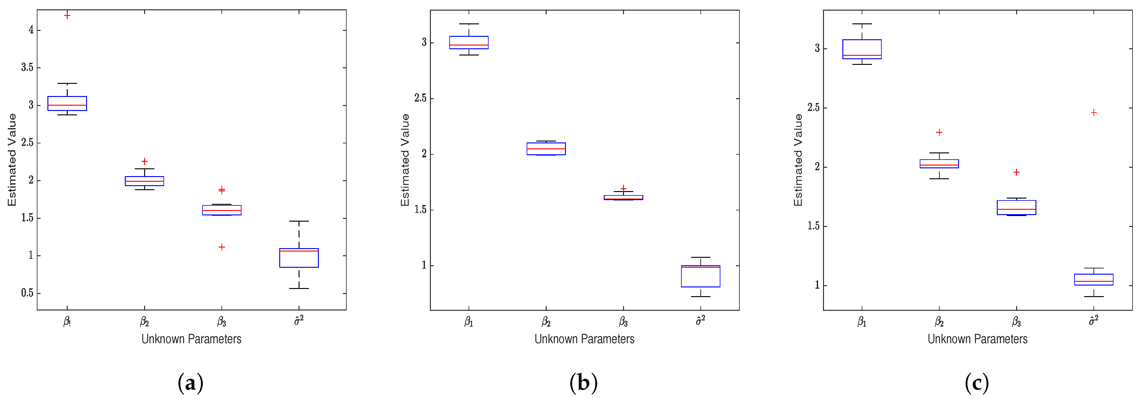
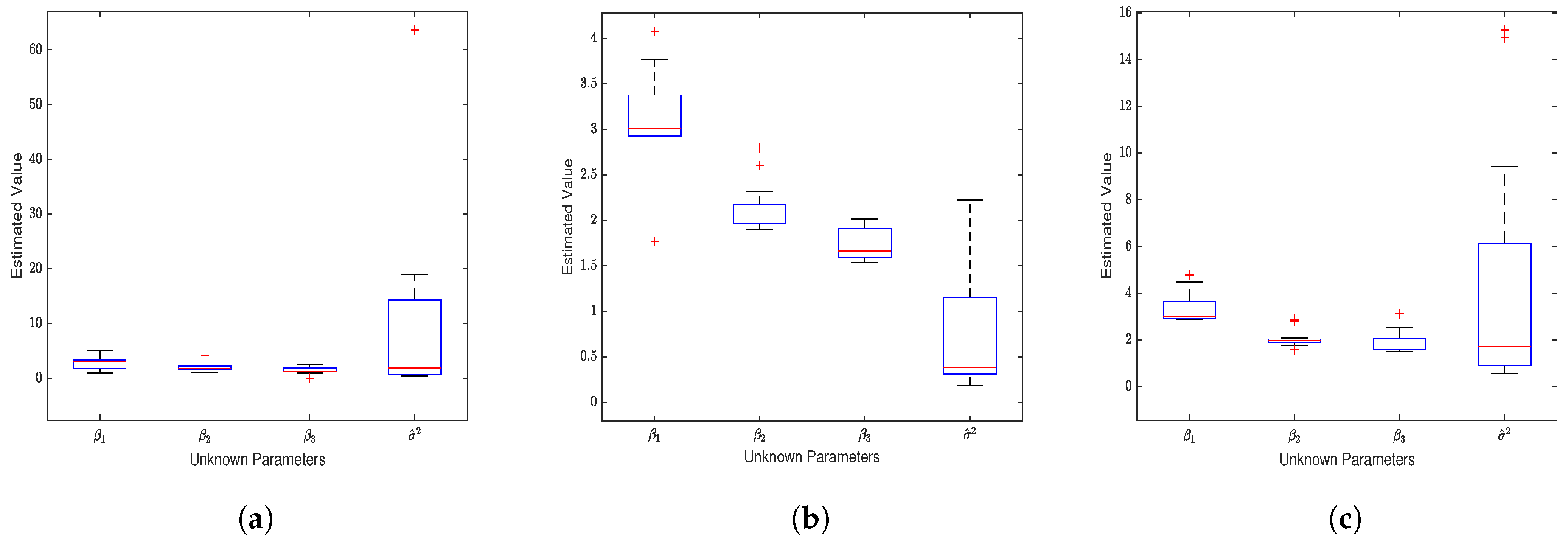
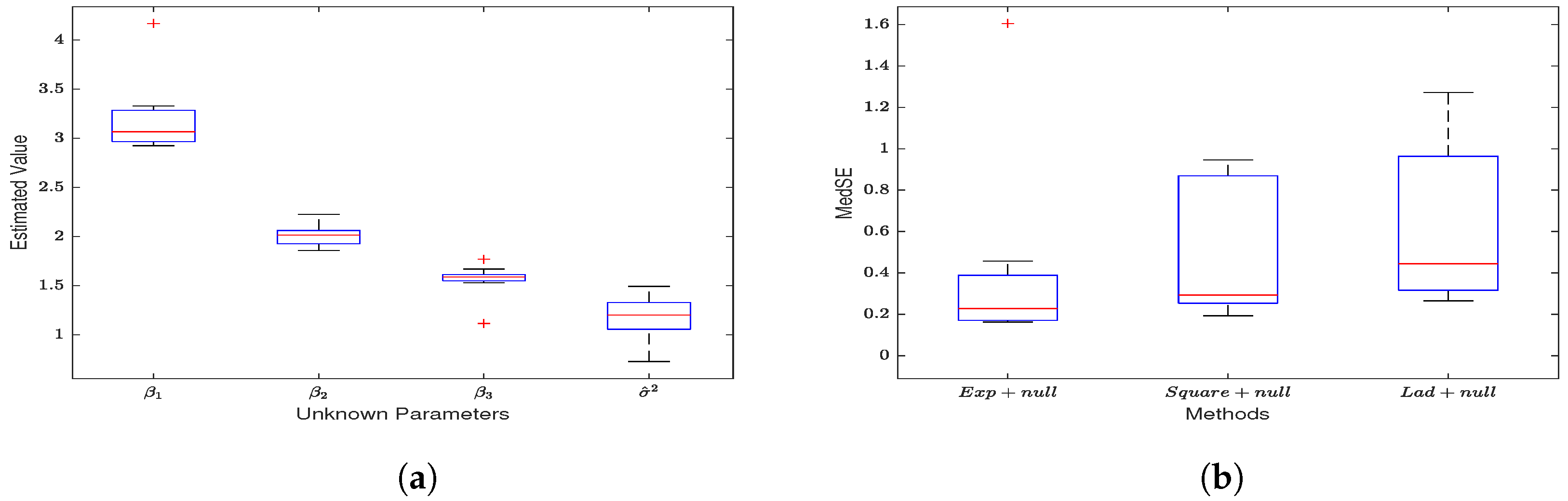
When considering the spatial effect of the error term (), the model’s estimation results are shown in Figure 1. (1) All three loss functions yield estimates of , and that closely align with their true values ( have means of 3, 2, 1.6, and the mean of is 1) as seen in Table A1. As the sample size increases, the estimates gradually converge to the true values. Notably, the square loss function provides the most accurate estimates. (2) When not considering the spatial effect of the response variable (), the SEM model also produces reasonably accurate estimates. However, ignoring the spatial effect of the error term () significantly reduces the accuracy of the SEM estimates. This is especially apparent in the estimation of the noise variance, and the estimates for and also become less accurate, resulting in an increase in MedSE. (3) According to Figure 2, by comparing the median squared error (MedSE), it is evident that the SEM model estimates based on the squared loss function perform the best in terms of estimation performance.
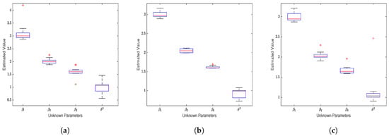
Figure 1.
Unregularized Estimation on Gaussian Noise Data (). (a) Estimates of the four unknown parameters in the SEM model based on the exponential squared loss function. (b) Estimates for the four unknown parameters based on the squared loss function. (c) Estimates for the unknown parameters based on the absolute value loss function.
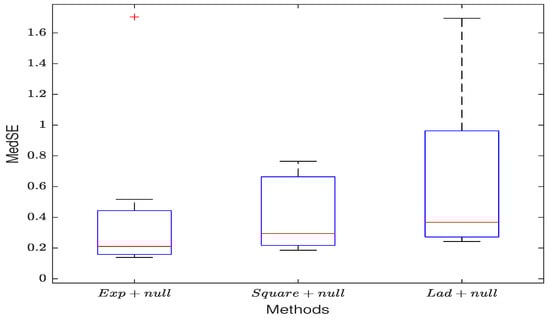
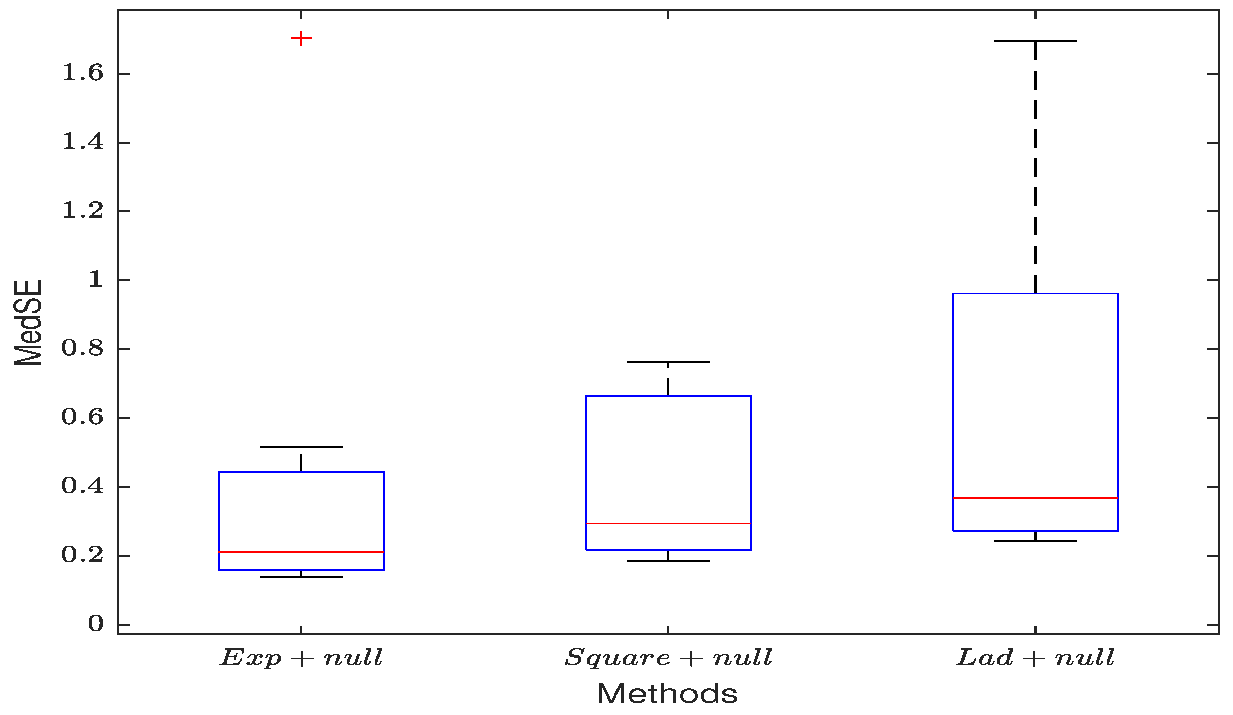
Figure 2.
The MedSE of the three unregularized loss function estimates.
The results in Figure 3 illustrate the estimation performance of the Structural Equation Modeling (SEM)model on normal data when there are numerous non-significant covariates. It is evident that the accuracy of the parameter estimates for the three loss functions is much lower than the results shown in Figure 1. Specifically, there are changes in the median values of parameter estimates and an increase in the number of outliers, with the exponential square loss function yielding the fewest outlier estimates. Examining the specific data in Table A2, it is observed that as the sample size increases, the estimates for parameters gradually approach the true values, and MedSE shows a decreasing trend. However, as anticipated, the results are still unsatisfactory.
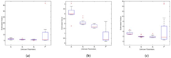
Figure 3.
Unregularized estimation on Gaussian noise data (). (a) Estimates of the four unknown parameters in the SEM model based on the exponential squared loss function. (b) Estimates for the four unknown parameters based on the squared loss function. (c) Estimates for the unknown parameters based on the absolute value loss function.
4.3. Unregularized Estimation When the Observed Values of Y Have Outliers
In this section, we use the SEM model to estimate the data with outliers in the response variable without regularization. (1) Similar to Table A1, all three loss functions provide reasonably accurate estimates for and , and as the sample size increases, the estimates get closer to the true values. Furthermore, the exponential loss, in particular, provides better estimates for and than the other two methods. (2) When ignoring the spatial effect of the model’s error term, the SEM estimates for the coefficients and noise variance are not accurate, and MedSE increases significantly compared to when . (3) By comparing Figure 1a with Figure 4a, it can be observed that the exponential square loss demonstrates better resistance to the influence of noise in the observed values. Additionally, through Figure 4b, similar results to Figure 2 can be observed, further highlighting the robustness advantage of the exponential square loss.
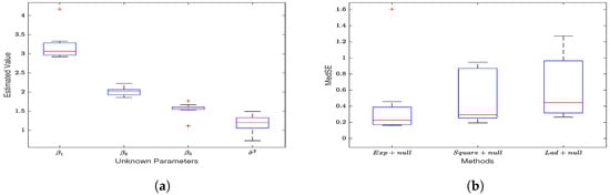
Figure 4.
Unregularized estimation when the observed values of y have outliers. (a) The estimation results of the non-regularized exponential square loss function. (b) The MedSE of the estimates for the three loss functions.
4.4. Unregularized Estimation with Noisy Spatial Weight Matrix
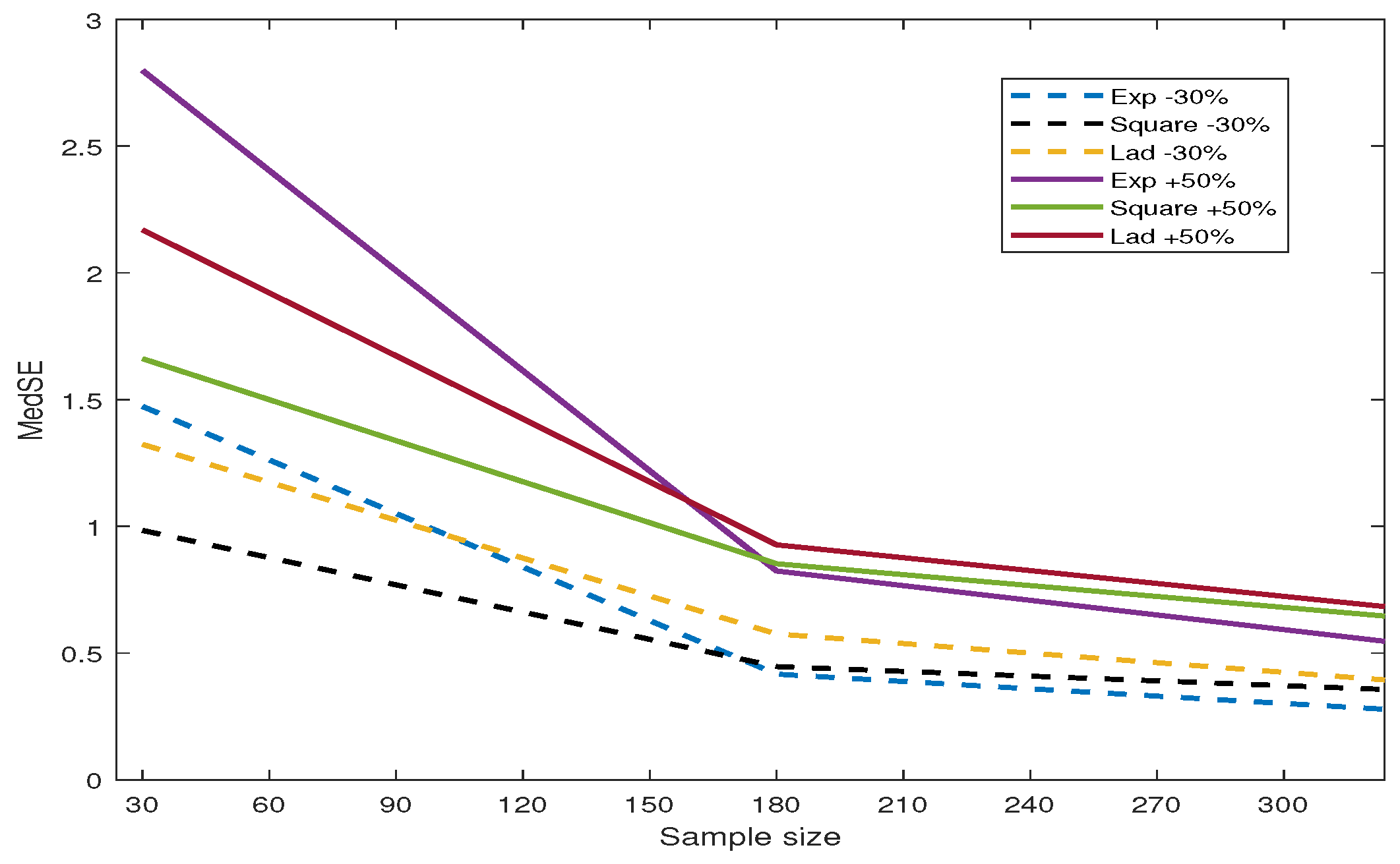
In this section, we designed an inaccurate spatial weight matrix and used the SEM model to estimate the coefficients and noise variance. “Remove 30% ” and “Add 50%” refer to randomly removing of non-zero values in each row of W and adding non-zero elements in each row, respectively. Table A4 presents the estimation results. All simulated data are generated based on and . Compared to the estimation results on normal data in Table A1, the inaccurate W leads to increased MedSE values and a decrease in the estimation performance for all three loss functions. To observe the variations in MedSE for each loss function, we plotted Figure 5. (1) When some non-zero weights in the matrix W are removed, the MedSE for all three loss functions decreases with an increase in the sample size. Among the three loss functions, the MedSE for the exponential square loss shows the most significant decrease, regardless of whether weights are added or removed. (2) When half of the non-zero weights in each row of W are added, all three methods have higher MedSE values compared to removing some non-zero weights from W. (3) Through the comparison of the estimated values and MedSE, we find that the exponential square loss shows more robustness when combating the impact of inaccurate spatial weight matrices.
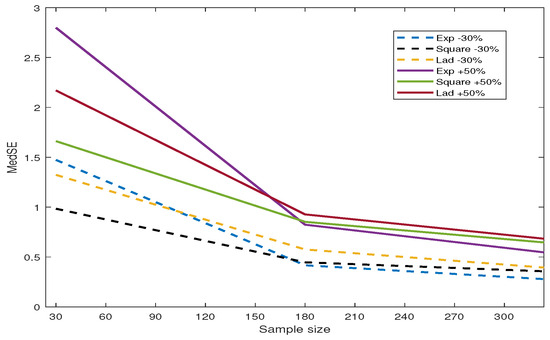
Figure 5.
The variation of MedSE with changes in sample size.
4.5. Variable Selection with Regularizer on Gaussian Noise Data
In this section, we perform variable selection on the generated Gaussian noise data (including and ) using the SEM model with three different loss functions and the penalty method (lasso or adaptive lasso). “Correct” represents the average number of correctly selected zero coefficients, and “InCorrect” represents the average number of non-zero coefficients incorrectly identified as zero. “Exp + l1 ”, “S + l1” and “Lad + l1” represent SEM models with exponential loss, square loss, and absolute loss, respectively, using the lasso penalty. “Exp + ”, “S + ” and “Lad + ” represent SEM models with exponential loss, square loss, and absolute loss, respectively, using the adaptive lasso penalty. The sample size for the variable selection simulation experiments is .
We visualized the results of variable selection for the model when considering the spatial effect of the error term and created Figure 6. (1) By observing Figure 6a, it is evident that the correctness of selecting non-zero regression coefficients for the three loss functions is relatively low when the sample size is small. Additionally, the loss functions incorporating the adaptive lasso penalty achieve higher accuracy in variable selection compared to those with the lasso penalty alone. As the sample size increases, all methods can almost correctly select all variables. A comparison reveals that the exponential square loss, combined with the adaptive lasso penalty, achieves higher accuracy. (2) The results in Figure 6b indicate that ignoring the spatial effect of the error term introduces significant disturbance to variable selection. The correctness of variable selection for all methods drops below half, and even with an increase in sample size, the improvement in variable selection is limited. However, through comparison, it is found that the exponential square loss exhibits the best robustness. (3) Combining with Table A5, it is observed that among the three loss functions, the SEM model with the exponential loss function has lower MedSE compared to the other two loss functions.
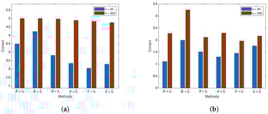
Figure 6.
The results of regularization variable selection based on normal data (). (a) Variable selection results for each method when . (b) Variable selection results for each method when .
Based on the variable selection structure when the number of non-significant covariates approaches the sample size, we plotted Figure 7. Due to the significant differences in variable selection results for different values of q (30 and 300), it is challenging to display them well in the graph. Therefore, we compared the variable selection differences for each method with or without considering the spatial effect of the error term. From Figure 7, it is evident that not considering the spatial effect of the error term significantly reduces the correct selection of variables. Table A6 presents the detailed results. Comparing with the results in Table A5, it is observed that when the sample size is small, using both lasso and adaptive lasso penalties with all three loss functions may lead to a slightly higher number of incorrect identifications of zero coefficients. However, as the sample size increases, the error rate decreases to zero. Importantly, the combination of the exponential square loss function with lasso and adaptive lasso penalties performs better in variable selection, ensuring smaller MedSE even when identifying more zero coefficients correctly. Similarly, ignoring the spatial effect of the error term leads to an increase in the error rate in variable selection for the SEM model, accompanied by an increase in MedSE.
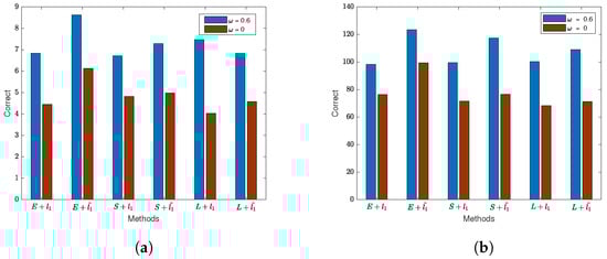
Figure 7.
The results of regularization variable selection based on normal data (). (a) Variable selection results for each method when . (b) Variable selection results for each method when .
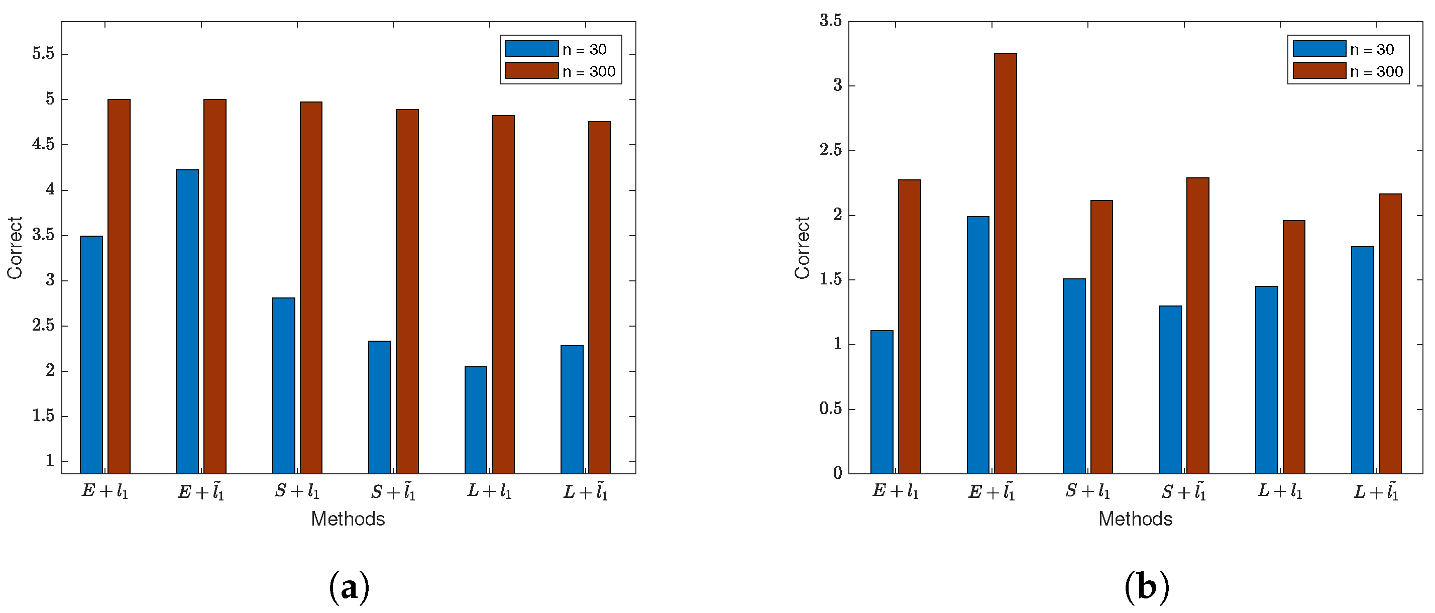
4.6. Variable Selection with Regularizer on Outlier Data
In order to compare the estimation and variable selection performance of various variable selection methods when data contain outliers, in this section, we conducted numerical simulations with response variable observations containing outliers and an inaccurate spatial weight matrix.
Table 1 presents the variable selection results of the SEM model when response variable observations contain outliers. We included data for sample sizes of 30 and 300, with . It can be observed that in almost all test cases, the SEM model with the exponential square loss and lasso or adaptive lasso penalties identifies more true zero coefficients and has a lower MedSE. Compared to the variable selection results for normal data in Table A5, the superiority of the exponential square loss with lasso and adaptive lasso penalties is more pronounced in the presence of outliers. It achieves higher accuracy in identifying zero coefficients and has lower MedSE. This indicates that the exponential square loss exhibits stronger robustness when outliers are present in Y. By observing the results for and , we can see that, similar to the results in Table A5 and Table A6, ignoring the spatial dependency in the error term often leads to a reduction in the number of correctly identified zero coefficients in the SEM model, decreased accuracy in identification, and an increase in MedSE.

Table 1.
Variable selection with regularizer when the observed values of y have outliers.
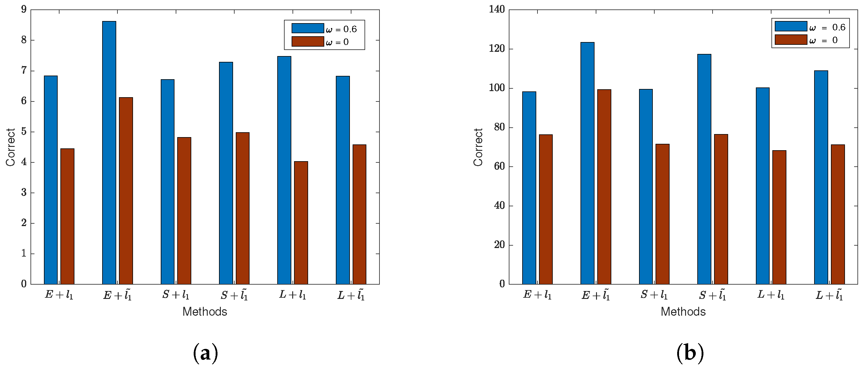
Table 2 presents the variable selection results in the case of inaccurate W. Because in practical applications it can be challenging to estimate the spatial weight matrix, this simulation provides valuable insights. In all test scenarios, the SEM model with the exponential square loss and lasso or adaptive lasso penalties achieves higher accuracy in identifying zero coefficients. In cases where of the non-zero values in W are removed and of non-zero values are added to W, the superiority of the proposed method becomes more apparent. It can correctly identify more zero coefficients while keeping MedSE smaller. In the presence of an inaccurate weight matrix, the impact of the spatial effects on the variable selection is similar to the results in Table A5 and Table A6, as well as Table 1. When , the SEM model incorrectly identifies a larger number of zero coefficients, but when , the number of incorrectly identified zero coefficients is reduced to zero. These results indicate that the proposed SEM variable selection method with the exponential square loss and lasso or adaptive lasso penalties is robust and suitable for variable selection in spatially dependent data, even when the weight matrix W cannot be accurately estimated.
Table 2.
Variable selection with regularizer with noisy W.
5. Empirical Data Verification
In this section, we apply the SEM variable selection method proposed in this paper to empirical dataset to verify the performance of parameter estimation and variable selection. The purpose of this experiment is to validate whether the proposed method can correctly select covariates that are useful for the response variable, according to Burnham and Andersen (2002) [19]. We choose BIC (Bayesian Information Criterion) as the criterion to assess the performance of the method. This paper uses the Boston Housing dataset, which was initially created by Harrison and Rubinfeld (1978 [20]). The data come from the real estate market in the Boston area in the 1970s and include information about housing prices in Massachusetts, USA. This dataset can be obtained from the “spdeep” library in R.
The Boston Housing dataset consists of 506 samples, each with 13 features and one response variable, making a total of 14 columns, Table 3 describes the meanings of various features in this dataset. The main objective is to study the relationship between housing prices and other variables and select the most important ones. The response variable is the logarithm of MEDV, and the predictor variables include the logarithm of DIS, RAD, LSTAT, as well as the square of RM and NOX. Other variables considered are CRIM, ZN, INDUS, CHAS, AGE, TAX, PTRATIO, and B-1000.
Table 3.
Variable description.
The spatial weight matrix W can be calculated based on the Euclidean distance using latitude and longitude coordinates. We set a distance threshold , and when the distance between two regions is greater than , . can be represented as:
Then, normalize each row of the spatial weight matrix W and incorporate it into the SEM model.
Table 4 presents the estimates and variable selection results for the SEM with three loss functions, lasso or adaptive lasso penalties, and no penalty. The results indicate that the SEM with all three loss functions provide estimates for and around 0.5 and 0.2, respectively. For variable selection, we consider a variable important when the absolute value of its coefficient estimate is greater than 0.05, while a variable is deemed unimportant when the absolute value of its coefficient estimate is less than 0.005. It can be observed that, in the absence of regularization terms, all three loss functions estimate the coefficients of NOX, DIS, RAD, and LSTAT to be greater than 0.05, classifying them as important variables. Moreover, all models suggest a negative correlation between NOX, DIS, LSTAT, and MEDV, indicating that higher nitrogen oxide concentrations, greater distances to employment centers, and a higher percentage of lower-income population are associated with lower housing prices. On the other hand, RAD is considered positively correlated with MEDV, implying that a higher highway accessibility index leads to higher housing prices in the area. However, INDUS, CHAS, and AGE are deemed unimportant variables, as their coefficient estimates have absolute values less than 0.005. ZN, TAX, and B-1000 have coefficient estimates close to zero. These findings suggest that the proposed method with the exponential square loss is effective in variable selection.
Table 4.
Variable selection for the Boston dataset.
To visually compare the variable selection performance with penalty terms for the three loss functions, we marked the variable selection results of the SEM model with “ + ” and “−” symbols. We set a threshold of 0.005, and variables with coefficients greater than 0.005 were marked with “ + ”, while those with coefficients less than −0.005 were marked with “−”. As shown in Table 5, the SEM models with the exponential square loss and adaptive lasso selected fewer variables. Furthermore, compared to the other two loss functions (with and without lasso penalties), the SEM model using adaptive lasso and exponential square loss has the lowest BIC index. This clearly demonstrates the superiority of the variable selection method proposed in this paper.
Table 5.
Variable selection for the Boston dataset after marking.
6. Conclusions and Discussions
The paper proposes a robust variable selection method for the spatial autoregressive model with exponential squared loss and the adaptive lasso penalty. This method can simultaneously select variables and estimate unknown coefficients. The main conclusions of this study are as follows:
- The penalized exponential squared loss effectively selects non-zero coefficients of covariates. When there is noise in the observations and an inaccurate spatial weight matrix, the proposed method shows significant resistance to their impact, demonstrating good robustness.
- The block coordinate descent (BCD) algorithm proposed in this work is effective in optimizing the penalized exponential squared loss function.
- In numerical simulation experiments and empirical applications, variable selection results with lasso and adaptive lasso penalties were compared, and adaptive lasso consistently outperformed in various scenarios.
- It is noteworthy that ignoring the spatial effects of error terms (i.e., ) severely reduces the accuracy of this variable selection method. However, for general error models (when , ), the proposed method remains applicable.
In the field of spatial econometrics, there are many other spatial regression models, as well as numerous robust loss functions and penalties. Building on the foundation of this study, we plan to explore more related issues in the future.
Author Contributions
Conceptualization, Y.S. and F.Z.; methodology, S.M.; software, S.M.; validation, Y.S.; formal analysis, Y.H.; investigation, F.Z.; resources, S.M.; writing—original draft preparation, S.M.; writing—review and editing, S.M., Y.H., Y.S. and F.Z.; supervision, Y.S.; project administration, S.M. All authors have read and agreed to the published version of the manuscript.
Funding
This work was supported by the Fundamental Research Funds for the Central Universities (No. 23CX03012A), National Key Research and Development Program (2021YFA1000102) of China, and Shandong Provincial Natural Science Foundation of China (ZR2021MA025, ZR2021MA028).
Institutional Review Board Statement
Not applicable.
Data Availability Statement
The authors confirm that the data supporting the findings of this study are cited within the manuscript.
Conflicts of Interest
The authors declare no conflicts of interest.
Appendix A
Appendix A provides specific data results for multiple scenarios in the numerical simulation experiments of Section 4 in this paper.
Table A1.
Unregularized estimation on normal data ().
Table A1.
Unregularized estimation on normal data ().
| n = 30, q = 5 | n = 150, q = 5 | n = 300, q = 5 | |||||||
| Exp | Square | LAD | Exp | Square | LAD | Exp | Square | LAD | |
| , | |||||||||
| 4.171 | 3.072 | 3.098 | 3.254 | 3.123 | 3.084 | 3.078 | 3.146 | 3.074 | |
| 2.259 | 2.012 | 2.312 | 1.974 | 2.109 | 2.171 | 2.138 | 2.086 | 2.061 | |
| 1.118 | 1.659 | 1.834 | 1.672 | 1.678 | 1.702 | 1.579 | 1.617 | 1.708 | |
| 0.742 | 0.786 | 0.734 | 0.797 | 0.796 | 0.788 | 0.792 | 0.798 | 0.795 | |
| 1.300 | 0.804 | 1.808 | 1.164 | 1.040 | 1.105 | 1.121 | 1.081 | 1.094 | |
| MedSE | 1.703 | 0.764 | 1.695 | 0.224 | 0.371 | 0.458 | 0.236 | 0.245 | 0.297 |
| , | |||||||||
| 3.114 | 2.939 | 2.898 | 3.094 | 2.987 | 2.911 | 2.935 | 3.042 | 3.024 | |
| 2.011 | 2.157 | 1.964 | 1.891 | 2.020 | 2.059 | 2.052 | 2.003 | 2.022 | |
| 1.646 | 1.622 | 1.739 | 1.607 | 1.578 | 1.580 | 1.542 | 1.565 | 1.629 | |
| 0.507 | 0.502 | 0.500 | 0.510 | 0.510 | 0.500 | 0.509 | 0.509 | 0.506 | |
| 0.557 | 0.735 | 0.947 | 1.098 | 0.981 | 0.966 | 1.066 | 1.030 | 1.045 | |
| MedSE | 0.398 | 0.703 | 0.964 | 0.176 | 0.290 | 0.357 | 0.140 | 0.188 | 0.244 |
| , | |||||||||
| 2.910 | 2.957 | 2.922 | 3.082 | 3.000 | 2.912 | 2.942 | 3.029 | 3.027 | |
| 2.004 | 2.156 | 1.931 | 1.891 | 2.050 | 2.063 | 2.056 | 2.012 | 2.047 | |
| 1.885 | 1.632 | 1.711 | 1.609 | 1.594 | 1.620 | 1.544 | 1.572 | 1.612 | |
| 0.058 | 0.016 | 0.054 | 0.006 | 0.002 | 0.007 | 0.000 | 0.000 | 0.007 | |
| 0.581 | 0.740 | 0.938 | 1.107 | 0.979 | 0.974 | 1.070 | 1.031 | 1.047 | |
| MedSE | 0.517 | 0.648 | 0.962 | 0.185 | 0.293 | 0.372 | 0.139 | 0.185 | 0.242 |
| , | |||||||||
| 4.294 | 2.237 | 2.721 | 2.528 | 2.567 | 1.751 | 1.212 | 1.820 | 1.942 | |
| 0.096 | 2.414 | 1.975 | 1.233 | 1.381 | 1.673 | −0.259 | 1.257 | 1.873 | |
| 2.146 | 1.226 | 1.898 | 0.244 | 1.457 | 1.447 | 1.089 | 1.216 | 0.794 | |
| 0.911 | 0.964 | 0.929 | 0.987 | 0.991 | 0.999 | 1.000 | 0.995 | 1.000 | |
| 13.450 | 7.520 | 5.206 | 55.573 | 15.911 | 31.349 | 32.997 | 67.428 | 15.859 | |
| MedSE | 3.484 | 4.041 | 8.717 | 2.598 | 3.896 | 5.733 | 4.231 | 5.101 | 6.523 |
| , | |||||||||
| 3.314 | 2.475 | 2.978 | 2.623 | 2.747 | 2.168 | 1.433 | 2.119 | 1.942 | |
| 0.282 | 2.319 | 1.865 | 1.418 | 1.429 | 1.963 | −0.407 | 1.558 | 1.298 | |
| 2.693 | 1.259 | 1.840 | 0.275 | 1.595 | 1.636 | 1.209 | 1.394 | 1.018 | |
| 0.860 | 0.921 | 0.832 | 0.955 | 0.953 | 0.996 | 0.984 | 0.964 | 1.000 | |
| 12.508 | 7.199 | 4.851 | 6.237 | 20.207 | 3.899 | 18.063 | 40.884 | 25.945 | |
| MedSE | 3.163 | 3.674 | 7.766 | 2.449 | 4.086 | 5.785 | 4.624 | 5.503 | 6.422 |
| , | |||||||||
| 3.943 | 2.692 | 3.217 | 3.176 | 3.330 | 2.444 | 1.827 | 2.874 | 1.896 | |
| 0.362 | 2.673 | 1.921 | 1.623 | 1.718 | 2.273 | −0.573 | 1.892 | 1.911 | |
| 2.994 | 1.392 | 1.646 | 0.314 | 1.997 | 1.623 | 1.401 | 1.618 | 1.010 | |
| 0.595 | 0.695 | 0.500 | 0.785 | 0.795 | 0.883 | 0.866 | 0.812 | 0.931 | |
| 17.035 | 37.543 | 42.054 | 28.235 | 29.141 | 58.824 | 13.277 | 12.483 | 13.397 | |
| MedSE | 3.593 | 4.421 | 7.071 | 2.809 | 4.954 | 6.589 | 5.417 | 6.489 | 9.667 |
Table A2.
Unregularized estimation on high-dimensional data ().
Table A2.
Unregularized estimation on high-dimensional data ().
| n = 30, q = 20 | n = 150, q = 100 | n = 300, q = 200 | |||||||
| Exp | Square | LAD | Exp | Square | LAD | Exp | Square | LAD | |
| , | |||||||||
| 1.099 | 3.608 | 4.362 | 3.558 | 3.666 | 4.079 | 4.763 | 3.673 | 4.484 | |
| 1.237 | 2.772 | 2.246 | 4.340 | 2.275 | 2.726 | 1.996 | 2.440 | 2.662 | |
| −0.108 | 1.765 | 2.791 | 1.618 | 1.829 | 2.114 | 1.889 | 1.959 | 2.162 | |
| 0.510 | 0.598 | 0.500 | 0.532 | 0.679 | 0.500 | 0.545 | 0.674 | 0.500 | |
| 45.621 | 1.288 | 6.188 | 8.776 | 1.492 | 11.372 | 7.246 | 1.937 | 10.486 | |
| MedSE | 11.084 | 7.086 | 12.913 | 9.651 | 4.764 | 9.521 | 9.006 | 4.919 | 9.523 |
| , | |||||||||
| 1.088 | 2.958 | 3.044 | 3.127 | 3.033 | 3.005 | 3.086 | 2.962 | 3.037 | |
| 1.500 | 1.958 | 1.849 | 2.023 | 1.999 | 1.959 | 2.173 | 1.984 | 1.976 | |
| 1.112 | 1.753 | 1.695 | 1.312 | 1.618 | 1.658 | 1.225 | 1.615 | 1.596 | |
| 0.505 | 0.502 | 0.500 | 0.502 | 0.505 | 0.500 | 0.509 | 0.504 | 0.500 | |
| 19.757 | 0.183 | 0.557 | 0.587 | 0.335 | 0.723 | 0.410 | 0.353 | 0.704 | |
| MedSE | 6.721 | 2.618 | 2.710 | 2.043 | 1.985 | 2.540 | 2.176 | 1.930 | 2.357 |
| , | |||||||||
| 2.530 | 2.940 | 3.104 | 3.187 | 2.946 | 2.956 | 2.851 | 2.925 | 2.858 | |
| 1.599 | 1.928 | 1.729 | 1.665 | 2.029 | 1.839 | 2.298 | 1.928 | 1.960 | |
| 1.964 | 1.804 | 1.844 | 1.250 | 1.546 | 1.485 | 1.246 | 1.568 | 1.517 | |
| 0.492 | 0.401 | 0.500 | 0.430 | 0.321 | 0.500 | 0.408 | 0.321 | 0.500 | |
| 0.229 | 0.239 | 1.066 | 0.986 | 0.383 | 1.295 | 0.507 | 0.404 | 1.469 | |
| MedSE | 5.446 | 3.522 | 4.221 | 2.856 | 2.264 | 3.505 | 2.477 | 2.228 | 3.432 |
| , | |||||||||
| 0.731 | 2.994 | 2.911 | 3.556 | 3.025 | 3.083 | 2.995 | 2.977 | 2.896 | |
| 1.535 | 1.908 | 1.939 | 1.641 | 2.073 | 1.861 | 2.320 | 1.990 | 2.067 | |
| 2.216 | 1.834 | 2.009 | 1.102 | 1.575 | 1.596 | 1.257 | 1.607 | 1.486 | |
| 0.476 | 0.164 | 0.500 | 0.336 | 0.109 | 0.500 | 0.148 | 0.083 | 0.500 | |
| 3.716 | 0.259 | 1.777 | 2.420 | 0.371 | 2.517 | 0.471 | 0.389 | 2.854 | |
| MedSE | 9.766 | 3.359 | 5.954 | 4.412 | 2.107 | 4.720 | 2.360 | 2.082 | 4.605 |
| , | |||||||||
| −4.722 | 2.551 | 6.874 | −2.831 | 3.651 | 7.391 | −0.018 | 2.533 | 4.660 | |
| 8.293 | 2.333 | 4.512 | −2.847 | 2.325 | 2.775 | 0.048 | 2.883 | 0.733 | |
| 3.117 | 1.760 | 2.022 | 4.418 | 0.425 | 6.648 | −0.110 | 1.959 | 5.006 | |
| 0.508 | 0.821 | 0.500 | 0.717 | 0.898 | 0.500 | 0.833 | 0.903 | 0.500 | |
| 27.293 | 20.282 | 24.512 | 17.575 | 19.964 | 22.157 | 9.306 | 13.666 | 16.381 | |
| MedSE | 39.686 | 27.898 | 67.610 | 35.056 | 35.448 | 31.470 | 14.067 | 13.665 | 25.497 |
| , | |||||||||
| −0.634 | 2.694 | 3.102 | −2.223 | 3.472 | 4.273 | −0.018 | 2.608 | 2.457 | |
| 3.128 | 1.900 | 3.563 | −3.418 | 1.873 | 0.452 | 0.048 | 2.129 | 1.651 | |
| 1.783 | 2.053 | 2.287 | 7.501 | 0.888 | 4.250 | −0.110 | 1.498 | 3.339 | |
| 0.506 | 0.767 | 0.500 | 0.674 | 0.858 | 0.500 | 0.604 | 0.868 | 0.500 | |
| 32.226 | 29.173 | 27.807 | 12.572 | 14.280 | 15.795 | 9.519 | 14.606 | 13.914 | |
| MedSE | 15.091 | 19.440 | 28.257 | 23.328 | 24.803 | 57.961 | 4.067 | 19.192 | 10.382 |
| , | |||||||||
| 0.333 | 2.403 | 3.076 | −1.754 | 3.674 | 3.566 | −0.018 | 2.733 | 3.423 | |
| 2.118 | 1.904 | 3.280 | −3.263 | 2.101 | 0.280 | 0.048 | 2.335 | 1.651 | |
| 1.454 | 2.556 | 2.786 | 8.025 | 1.190 | 3.249 | −0.110 | 1.360 | 3.278 | |
| 0.499 | 0.655 | 0.500 | 0.603 | 0.801 | 0.500 | 0.390 | 0.805 | 0.500 | |
| 20.537 | 17.192 | 33.633 | 21.775 | 23.257 | 26.938 | 25.876 | 15.694 | 84.560 | |
| MedSE | 10.570 | 18.943 | 18.371 | 24.953 | 26.615 | 14.682 | 14.067 | 14.201 | 18.278 |
| , | |||||||||
| 0.271 | 2.498 | 3.162 | −1.888 | 3.922 | 3.214 | −0.018 | 2.932 | 4.047 | |
| 1.934 | 1.877 | 1.642 | −2.505 | 2.193 | 0.938 | 0.048 | 2.427 | 1.655 | |
| 1.054 | 2.561 | 1.787 | 3.895 | 1.224 | 3.179 | −0.110 | 1.403 | 1.953 | |
| 0.497 | 0.546 | 0.500 | 0.545 | 0.690 | 0.500 | 0.382 | 0.714 | 0.500 | |
| 25.288 | 21.138 | 30.855 | 25.724 | 62.474 | 21.793 | 52.331 | 16.704 | 7.310 | |
| MedSE | 10.854 | 19.911 | 17.329 | 14.779 | 18.196 | 22.821 | 14.067 | 11.641 | 18.816 |
Table A3.
Unregularized estimation when the observed values of y have outliers.
Table A3.
Unregularized estimation when the observed values of y have outliers.
| n = 30, q = 5 | n = 150, q = 5 | n = 300, q = 5 | |||||||
| Exp | Square | LAD | Exp | Square | LAD | Exp | Square | LAD | |
| , | |||||||||
| 4.053 | 3.151 | 3.030 | 3.321 | 3.111 | 3.131 | 3.048 | 3.145 | 3.161 | |
| 2.184 | 2.032 | 2.203 | 1.929 | 2.105 | 2.104 | 2.111 | 2.083 | 2.102 | |
| 1.146 | 1.726 | 1.790 | 1.661 | 1.701 | 1.642 | 1.592 | 1.700 | 1.710 | |
| 0.730 | 0.768 | 0.736 | 0.781 | 0.784 | 0.779 | 0.779 | 0.786 | 0.775 | |
| 1.228 | 0.953 | 1.509 | 1.362 | 1.126 | 1.265 | 1.214 | 1.174 | 1.225 | |
| MedSE | 1.605 | 0.945 | 1.272 | 0.280 | 0.394 | 0.537 | 0.228 | 0.270 | 0.329 |
| , | |||||||||
| 3.261 | 2.997 | 3.053 | 3.126 | 2.942 | 3.029 | 2.926 | 2.960 | 2.978 | |
| 2.001 | 1.957 | 2.074 | 1.877 | 2.023 | 2.010 | 2.042 | 1.997 | 1.997 | |
| 1.531 | 1.569 | 1.641 | 1.601 | 1.627 | 1.504 | 1.557 | 1.632 | 1.596 | |
| 0.513 | 0.520 | 0.500 | 0.525 | 0.512 | 0.510 | 0.529 | 0.524 | 0.531 | |
| 0.751 | 0.837 | 0.975 | 1.328 | 1.072 | 1.170 | 1.184 | 1.119 | 1.185 | |
| MedSE | 4.456 | 4.861 | 4.920 | 3.173 | 3.293 | 4.445 | 1.163 | 2.204 | 3.278 |
| , | |||||||||
| 3.103 | 2.376 | 3.016 | 2.991 | 2.348 | 2.567 | 1.889 | 2.577 | 1.983 | |
| 2.795 | 1.830 | 1.158 | 1.848 | 1.209 | 2.053 | 1.386 | 1.406 | 2.538 | |
| 0.701 | 1.062 | 0.921 | 0.067 | 1.317 | 0.839 | 1.237 | 1.594 | 1.130 | |
| 0.821 | 0.983 | 0.922 | 0.988 | 0.991 | 0.993 | 0.999 | 0.993 | 1.000 | |
| 22.181 | 24.467 | 26.215 | 12.463 | 20.053 | 24.074 | 4.611 | 3.030 | 4.237 | |
| MedSE | 5.652 | 3.988 | 8.597 | 3.345 | 3.917 | 6.431 | 1.427 | 3.925 | 6.045 |
Table A4.
Unregularized estimation with noisy W.
Table A4.
Unregularized estimation with noisy W.
| n = 30, q = 5 | n = 150, q = 5 | n = 300, q = 5 | |||||||
| Exp | Square | LAD | Exp | Square | LAD | Exp | Square | LAD | |
| Remove 30% | |||||||||
| , | |||||||||
| 2.354 | 2.881 | 3.018 | 3.018 | 3.122 | 3.127 | 3.037 | 3.090 | 3.127 | |
| 2.987 | 2.073 | 1.746 | 1.912 | 2.077 | 1.971 | 2.202 | 2.009 | 2.021 | |
| 1.239 | 1.620 | 1.547 | 1.791 | 1.698 | 1.552 | 1.529 | 1.693 | 1.656 | |
| 0.461 | 0.436 | 0.499 | 0.417 | 0.387 | 0.410 | 0.385 | 0.399 | 0.396 | |
| 1.457 | 1.266 | 1.811 | 1.340 | 1.313 | 1.362 | 1.367 | 1.377 | 1.332 | |
| MedSE | 1.473 | 0.984 | 1.323 | 0.417 | 0.447 | 0.575 | 0.272 | 0.353 | 0.386 |
| Remove 30% | |||||||||
| , | |||||||||
| 2.950 | 2.223 | 2.784 | 2.058 | 2.485 | 2.845 | 1.364 | 2.763 | 2.652 | |
| 1.032 | 2.676 | 2.846 | 2.162 | 1.694 | 1.471 | 0.513 | 1.640 | 1.773 | |
| 1.381 | 1.138 | 0.034 | −0.095 | 1.204 | 2.104 | 1.350 | 1.173 | 1.009 | |
| 0.880 | 0.860 | 0.744 | 0.893 | 0.927 | 0.907 | 0.938 | 0.933 | 0.933 | |
| 16.184 | 21.415 | 28.473 | 19.800 | 33.276 | 36.677 | 15.618 | 23.684 | 29.837 | |
| MedSE | 3.155 | 4.693 | 9.478 | 2.925 | 5.896 | 8.407 | 3.934 | 7.624 | 9.886 |
| Add 50% | |||||||||
| , | |||||||||
| 4.936 | 3.286 | 3.396 | 3.649 | 3.266 | 3.365 | 3.334 | 3.379 | 3.279 | |
| 1.816 | 2.287 | 2.220 | 2.120 | 2.220 | 2.092 | 2.103 | 2.167 | 2.210 | |
| 0.613 | 1.907 | 1.653 | 1.990 | 1.756 | 1.779 | 1.729 | 1.772 | 1.896 | |
| 0.381 | 0.425 | 0.500 | 0.364 | 0.415 | 0.443 | 0.408 | 0.419 | 0.430 | |
| 2.532 | 1.972 | 2.801 | 1.963 | 1.540 | 1.640 | 1.436 | 1.511 | 1.589 | |
| MedSE | 2.799 | 1.662 | 2.170 | 0.824 | 0.852 | 0.927 | 0.535 | 0.637 | 0.673 |
Table A5.
Variable selection with regularizer on normal data ().
Table A5.
Variable selection with regularizer on normal data ().
| n = 30, q = 5 | n = 300, q = 5 | |||||||||||
|---|---|---|---|---|---|---|---|---|---|---|---|---|
| Exp + l1 | Exp + | S + l1 | S + | Lad + l1 | Lad + | Exp + l1 | Exp + | S + l1 | S + | Lad + l1 | Lad + | |
| Correct | 1.80 | 2.17 | 2.20 | 2.10 | 1.57 | 1.77 | 5.00 | 5.00 | 4.90 | 4.87 | 4.87 | 4.57 |
| Incorrect | 0.00 | 0.00 | 0.00 | 0.00 | 0.03 | 0.00 | 0.00 | 0.00 | 0.00 | 0.00 | 0.00 | 0.00 |
| MedSE | 1.50 | 1.48 | 1.01 | 0.85 | 1.41 | 1.43 | 0.23 | 0.22 | 0.27 | 0.25 | 0.30 | 0.33 |
| Correct | 4.17 | 4.87 | 2.90 | 2.40 | 2.57 | 2.70 | 5.00 | 5.00 | 5.00 | 4.90 | 4.80 | 4.83 |
| Incorrect | 0.00 | 0.00 | 0.00 | 0.00 | 0.00 | 0.00 | 0.00 | 0.00 | 0.00 | 0.00 | 0.00 | 0.00 |
| MedSE | 0.38 | 0.25 | 0.60 | 0.71 | 0.82 | 0.74 | 0.13 | 0.11 | 0.24 | 0.22 | 0.24 | 0.28 |
| Correct | 4.03 | 5.00 | 3.10 | 2.37 | 1.83 | 2.17 | 5.00 | 5.00 | 5.00 | 4.90 | 4.80 | 4.83 |
| Incorrect | 0.00 | 0.00 | 0.00 | 0.00 | 0.00 | 0.00 | 0.00 | 0.00 | 0.00 | 0.00 | 0.00 | 0.00 |
| MedSE | 0.44 | 0.16 | 0.60 | 0.77 | 1.00 | 0.98 | 0.13 | 0.11 | 0.23 | 0.20 | 0.28 | 0.26 |
| Correct | 1.57 | 3.03 | 0.60 | 0.40 | 0.40 | 0.67 | 3.07 | 3.00 | 0.47 | 0.33 | 0.47 | 0.47 |
| Incorrect | 0.67 | 1.00 | 0.10 | 0.13 | 0.07 | 0.27 | 1.73 | 1.67 | 0.07 | 0.13 | 0.27 | 0.27 |
| MedSE | 3.39 | 3.72 | 3.65 | 3.92 | 6.13 | 5.26 | 3.89 | 3.90 | 5.36 | 5.92 | 5.54 | 6.81 |
| Correct | 0.90 | 3.00 | 0.50 | 0.20 | 0.37 | 0.77 | 2.10 | 2.00 | 0.43 | 0.20 | 0.57 | 0.67 |
| Incorrect | 0.00 | 0.00 | 0.10 | 0.10 | 0.10 | 0.17 | 1.07 | 1.00 | 0.03 | 0.00 | 0.17 | 0.27 |
| MedSE | 2.44 | 2.71 | 3.87 | 4.13 | 4.31 | 4.51 | 4.19 | 4.34 | 5.77 | 6.32 | 5.44 | 6.21 |
| Correct | 1.00 | 2.97 | 0.50 | 0.33 | 0.63 | 0.87 | 1.97 | 2.00 | 0.40 | 0.33 | 0.30 | 0.40 |
| Incorrect | 0.00 | 0.00 | 0.13 | 0.17 | 0.10 | 0.17 | 0.97 | 1.00 | 0.10 | 0.03 | 0.13 | 0.17 |
| MedSE | 2.63 | 3.21 | 4.36 | 4.50 | 4.36 | 4.67 | 4.65 | 4.94 | 6.77 | 7.52 | 7.04 | 7.67 |
Table A6.
Variable selection with regularizer on high-dimensional data ().
Table A6.
Variable selection with regularizer on high-dimensional data ().
| n = 30, q = 20 | n = 300, q = 200 | |||||||||||
| Exp + l1 | Exp + | S + l1 | S + | Lad + l1 | Lad + | Exp + l1 | Exp + | S + l1 | S + | Lad + l1 | Lad + | |
| Correct | 3.4 | 4.9 | 1.2 | 2.7 | 4.5 | 5.8 | 94.5 | 135.0 | 89.1 | 89.2 | 96.6 | 103.0 |
| Incorrect | 0.2 | 0.5 | 0.0 | 0.1 | 0.0 | 0.1 | 0.0 | 0.0 | 0.0 | 0.0 | 0.0 | 0.0 |
| MedSE | 7.4 | 7.2 | 9.0 | 7.0 | 3.4 | 3.8 | 4.3 | 2.8 | 4.9 | 5.1 | 4.2 | 4.3 |
| Correct | 5.2 | 8.3 | 4.8 | 5.3 | 10.3 | 11.6 | 178.0 | 198.0 | 170.0 | 166.0 | 188.0 | 191.0 |
| Incorrect | 0.2 | 0.2 | 0.0 | 0.0 | 0.0 | 0.0 | 0.0 | 0.0 | 0.0 | 0.0 | 0.0 | 0.0 |
| MedSE | 4.8 | 2.2 | 3.1 | 2.5 | 1.5 | 1.4 | 1.7 | 0.9 | 2.0 | 2.1 | 1.5 | 1.4 |
| Correct | 4.8 | 6.1 | 4.2 | 4.3 | 6.9 | 8.2 | 180.2 | 200.0 | 165.3 | 158.4 | 153.8 | 156.6 |
| Incorrect | 0.1 | 0.1 | 0.1 | 0.0 | 0.0 | 0.0 | 0.0 | 0.0 | 0.0 | 0.0 | 0.0 | 0.0 |
| MedSE | 5.6 | 4.3 | 3.6 | 3.5 | 2.1 | 2.1 | 1.8 | 0.9 | 2.1 | 2.2 | 2.4 | 2.3 |
| Correct | 5.5 | 8.0 | 0.7 | 0.6 | 1.1 | 2.4 | 20.0 | 20.0 | 7.7 | 6.6 | 4.1 | 10.1 |
| Incorrect | 1.1 | 1.6 | 0.0 | 0.0 | 0.1 | 0.2 | 3.0 | 3.0 | 0.1 | 0.0 | 0.1 | 0.0 |
| MedSE | 18.9 | 20.4 | 23.7 | 25.9 | 18.4 | 13.7 | 4.1 | 4.1 | 94.6 | 80.2 | 145.0 | 155.2 |
| Correct | 3.6 | 4.7 | 0.8 | 0.9 | 2.1 | 3.4 | 19.6 | 20.0 | 9.8 | 10.5 | 9.6 | 13.7 |
| Incorrect | 0.2 | 0.8 | 0.1 | 0.0 | 0.1 | 0.2 | 2.9 | 3.0 | 0.1 | 0.1 | 0.0 | 0.1 |
| MedSE | 11.3 | 12.3 | 14.8 | 18.9 | 8.3 | 7.8 | 4.1 | 4.1 | 6.3 | 5.3 | 6.2 | 5.6 |
| Correct | 3.8 | 4.8 | 0.9 | 1.5 | 2.6 | 3.8 | 19.6 | 20.0 | 9.2 | 8.7 | 12.6 | 14.8 |
| Incorrect | 0.1 | 0.5 | 0.3 | 0.1 | 0.1 | 0.2 | 2.9 | 3.0 | 0.1 | 0.0 | 0.1 | 0.1 |
| MedSE | 8.6 | 8.9 | 14.8 | 18.9 | 6.4 | 6.8 | 4.1 | 4.1 | 6.4 | 5.9 | 4.3 | 3.6 |
Appendix B
Appendix B provides the derivation of the computational complexity of the BCD algorithm designed in Section 3, along with the specifications of the machine used to execute the program designed in this paper. This includes relevant hardware configurations, the operating system, and the programming software employed.
According to the study by Beck and Teboulle (2009) [17], the FISTA algorithm converges to the optimal solution at a rate of when solving problem (22), where k is the iteration step. Since the termination conditions of Algorithm 1 are or , to obtain an -optimal solution, the FISTA algorithm requires iterations, where each iteration is used to calculate the gradient of (23). As the computation is needed to calculate the , the computation paid for an -optimal solution of the subproblem (22) is . We assume that the BCD algorithm converges within a specified number of iterations, and in each iteration, the CCCP algorithm terminates at a maximum iteration number of . The total computational complexity of the algorithm is then .
The computer used in this experiment is equipped with an Intel Core i7 processor, 16 GB of RAM, and a 1 TB hard drive, running on a Windows 10 workstation. We implemented the designed algorithm using MATLAB R2020a and subsequently visualized the results.
References
- Anselin, L. Spatial Econometrics: Methods and Models; Springer Science and Business Media: Berlin/Heidelberg, Germany, 1988. [Google Scholar]
- Tibshirani, R. Regression shrinkage and selection via the lasso. J. R. Stat. Soc. Ser. B Stat. Methodol. 1996, 58, 267–288. [Google Scholar] [CrossRef]
- Fan, J.; Li, R. Variable selection via nonconcave penalized likelihood and its oracle properties. J. Am. Stat. Assoc. 2001, 96, 1348–1360. [Google Scholar] [CrossRef]
- Zou, H. The adaptive lasso and its oracle properties. J. Am. Stat. Assoc. 2006, 101, 1418–1429. [Google Scholar] [CrossRef]
- Huber, P.J. Robust Statistics; John Wiley Sons: Hoboken, NJ, USA, 2004. [Google Scholar]
- Wang, X.; Jiang, Y.; Huang, M.; Zhang, H. Robust variable selection with exponential squared loss. J. Am. Stat. Assoc. 2013, 108, 632–643. [Google Scholar] [CrossRef] [PubMed]
- Koenker, R.; Bassett, G., Jr. Regression quantiles. Econom. J. Econom. Soc. 1978, 46, 33–50. [Google Scholar] [CrossRef]
- Zou, H.; Yuan, M. Composite quantile regression and the oracle model selection theory. Ann. Statist. 2008, 36, 1108–1126. [Google Scholar] [CrossRef]
- Liu, X.; Ma, H.; Deng, S. Variable Selection for Spatial Error Models. J. Yanbian Univ. Nat. Sci. Ed. 2020, 46, 15–19. [Google Scholar]
- Doğan, O. Modified harmonic mean method for spatial autoregressive models. Econ. Lett. 2023, 223, 110978. [Google Scholar] [CrossRef]
- Song, Y.; Liang, X.; Zhu, Y.; Lin, L. Robust variable selection with exponential squared loss for the spatial autoregressive model. Comput. Stat. Data Anal. 2021, 155, 107094. [Google Scholar] [CrossRef]
- Banerjee, S.; Carlin, B.P.; Gelfand, A.E. Hierarchical Modeling and Analysis for Spatial Data; CRC Press: Boca Raton, FL, USA, 2014. [Google Scholar]
- Ma, Y.; Pan, R.; Zou, T.; Wang, H. A naive least squares method for spatial autoregression with covariates. Stat. Sin. 2020, 30, 653–672. [Google Scholar] [CrossRef]
- Wang, H.; Li, G.; Jiang, G. Robust regression shrinkage and consistent variable selection through the LAD-Lasso. J. Bus. Econ. Stat. 2007, 25, 347–355. [Google Scholar] [CrossRef]
- Forsythe, G.E. Computer Methods for Mathematical Computations; Prentice-Hall: Hoboken, NJ, USA, 1977. [Google Scholar]
- Yuille, A.L.; Rangarajan, A. The concave-convex procedure. Neural Comput. 2003, 15, 915–936. [Google Scholar] [CrossRef] [PubMed]
- Beck, A.; Teboulle, M. A fast iterative shrinkage-thresholding algorithm for linear inverse problems. SIAM J. Imaging Sci. 2009, 2, 183–202. [Google Scholar] [CrossRef]
- Liang, H.; Li, R. Variable selection for partially linear models with measurement errors. J. Am. Stat. Assoc. 2009, 104, 234–248. [Google Scholar] [CrossRef] [PubMed]
- Burnham, K.P.; Anderson, D.R. Model Selection and Multimodel Inference. A Practical Information-Theoretic Approach; Springer: Berlin/Heidelberg, Germany, 2004; Volume 2. [Google Scholar]
- Harrison, D., Jr.; Rubinfeld, D.L. Hedonic housing prices and the demand for clean air. J. Environ. Econ. Manag. 1978, 5, 81–102. [Google Scholar] [CrossRef]
Disclaimer/Publisher’s Note: The statements, opinions and data contained in all publications are solely those of the individual author(s) and contributor(s) and not of MDPI and/or the editor(s). MDPI and/or the editor(s) disclaim responsibility for any injury to people or property resulting from any ideas, methods, instructions or products referred to in the content. |
© 2023 by the authors. Licensee MDPI, Basel, Switzerland. This article is an open access article distributed under the terms and conditions of the Creative Commons Attribution (CC BY) license (https://creativecommons.org/licenses/by/4.0/).