Abstract
(1) Background: A new probabilistic physico-chemical model of the drifting key parameter of measuring equipment is proposed. The model allows for the integrated consideration of degradation processes (electrolytic corrosion, oxidation, plastic accumulation of dislocations, etc.) in nodes and elements of measuring equipment. The novelty of this article lies in the analytical solutions that are a combination of the Fokker–Planck–Kolmogorov equation and the equation of chemical kinetics. The novelty also consists of the simultaneous simulation and analysis of probabilistic, physical and chemical processes in one model. (2) Research literature review: Research works related to the topic of the study were analyzed. The need for a probabilistic formulation of the problem is argued, since classical statistical methods are not applicable due to the lack of statistical data. (3) Statement of the research problem: A probabilistic formulation of the problem is given taking into account the physical and chemical laws of aging and degradation. (4) Methods: The author uses methods of probability theory and mathematical statistics, methods for solving the stochastic differential equations, the methods of mathematical modeling, the methods of chemical kinetics and the methods for solving a partial differential equations. (5) Results: A mathematical model of a drifting key parameter of measuring equipment is developed. The conditional transition density of the probability distribution of the key parameter of measuring equipment is constructed using a solution to the Fokker–Planck–Kolmogorov equation. The results of the study on the developed model and the results of solving the applied problem of constructing the function of the failure rate of measuring equipment are presented. (6) Discussion: The results of comparison between the model developed in this paper and the known two-parameter models of diffusion monotonic distribution and diffusion non-monotonic distribution are discussed. The results of comparison between the model and the three-parameter diffusion probabilistic physical model developed by the author earlier are also discussed. (7) Conclusions: The developed model facilitates the construction and analysis of a wide range of metrological characteristics such as measurement errors and measurement ranges and acquisition of their statistical estimates. The developed model is used to forecast and simulate the reliability of measuring equipment in general, as well as soldered joints of integrated circuits in special equipment and machinery, which is also operated in harsh conditions and corrosive environments.
Keywords:
diffusion model; physical chemistry; chemical kinetics; measuring equipment; probability density function MSC:
90B25; 60-02
1. Introduction
The analysis of reliability, serviceability, reliability and durability is an integral part of development and operation of high-tech products [1,2,3,4,5,6,7].
It is experimentally proved that the discrepancy in the estimation of reliability values of complex technical systems, depending on the traditional theoretical model, can differ by a factor of 10–30 times. Hence, the choice of this or that theoretical model of element failure distribution ultimately determines the corresponding accuracy of calculated reliability values for the technical devices and systems being developed.
Many branches of mathematics, including the theory of continuous Markovian diffusion processes [8,9,10,11,12,13], the theory of differential equations [14], probabilistic physical diffusion and physico-statistical models [15,16,17,18,19], are used to develop methods for calculating reliability, serviceability and failure-free operation. In [15], the technology of development of diffusion models is described, including monotonic diffusion (MD) and non-monotonic diffusion (ND) distributions, which belong to the class of probabilistic physical models.
In works [16,17,18], the results of the simulation and application of a probabilistic physical diffusion model in medicine are considered. These works also address the estimation of the maximum possible load on human joints and the musculoskeletal system.
In [19,20], the results of application of a probabilistic physical model to statistical estimations of the key parameter (KP) in metrological support tasks are presented.
The correct selection of a theoretical model of the failure distribution for high-reliability specimens of measuring equipment (ME) [8,9,10,11], which include electronic components (integrated circuits, semiconductors, chips, soldered joints, etc.), as well as components of mechatronic systems, turns out to be a difficult task. If for mechanical objects and systems the correctness of the choice of the theoretical model can be checked using statistical methods, in the case of the above ME, including integrated circuits and mechatronic components, soldered joints, etc., the task is much more complicated. It seems to be impossible and unproductive to obtain complete statistical cases of ME failures even in forced ME test modes. Therefore, standard statistical methods based on the known statistical criteria of agreement (chi-square criterion, omega-square criterion, Kolmogorov’s criterion, etc.) appear to be unproductive.
One of the promising directions of choosing a theoretical model of ME failure distribution is the choice made on the basis of physical and chemical justification of the processes occurring in ME nodes and elements. Hence, only a thorough study of the cause-and-effect mechanisms of degradation (aging) and consideration of physical and chemical processes of ME degradation (aging) will identify the best model of failure distribution.
In Section 2, we provide a review of the research literature and a retrospective analysis of ME failure models. In Section 3, we formulate the statement of the research problem. In Section 4, we describe methods for constructing the probabilistic physico-chemical diffusion model. In Section 5, we describe the findings of the model research and application to the practical problem of constructing the function of the ME failure rate.
2. Research Literature Review
2.1. Alpha-Distribution
One of the first attempts to describe the KP behavior and formalize the model of parametric failures was an attempt to present the KP drift as a linear function shown in Figure 1. This distribution law is called alpha-distribution.
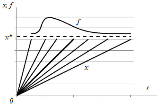
Figure 1.
The random degradation process model and the scheme of the time before failure distribution formation (alpha-distribution).
The solution to the failure formalization problem in the case of the alpha-distribution of a process is reduced to a J.K. Kapteyn scheme [15], when experimental data are compared with such a distribution of a random variable that some function on has a normal normalized law [20]:
where a lower index indicates that this is the alpha-distribution law; is the normal normalized law distribution function (Laplace function); is the function of the distribution density for the normal normalized law (cumulative distribution function); is the pre-set limit value of KP leading to the failure state; is the mean of rate of the KP change normalized to the ultimate value ; is the coefficient of variation of the rate of the KP change.
2.2. First Type of Normal Parametric Distribution
When considering a stationary wear process, during which KP changed in proportion to time, the authors [5] used the hypothesis of a strong mixing wear process, and the distribution of the operating time before failure was asymptotically normal for large values of wear (Figure 2):
where a lower index indicates that this is the first type of the normal distribution law; is the distribution function of the normal normalized law described above.
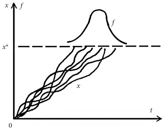
Figure 2.
The random degradation process model (the strong mixing Gaussian process) and the scheme of the time before failure distribution formation (normal parametric distribution).
It should be noted that the assumption of a linear relationship between a change in the defining parameter and time does not correspond to empirical data and is incorrect from a mathematical point of view.
It is known that for the stationary wear process, a change in the wear is proportional to the square of time. The erroneous attempt of the authors of work [5] to fit the distribution of wear failures into the framework of the normal distribution law has led to the failure to comply with the dimensionality of the argument of function .
2.3. Second Type of Normal Parametric Distribution
The distribution of time before failure is assumed to be normal:
where a lower index indicates that this is the second type of the normal distribution law, is the normal normalized law distribution function described above, and and are the mean value and standard deviation of mean time before failure, respectively.
The relationship between the parameters of this distribution and the characteristics of the wear and aging process is identified using the following simple considerations. The average operating time is related to the average wear and aging rate as . The value of the second parameter is determined using the assumption of equality of the variation coefficients of the degradation process and the distribution of the operating time before failure: . By substituting these values, we obtain:
We can see that the argument of the above expression differs from argument of function .
It should be noted that formalization schemes for probabilistic reliability models , , have no mathematical rigor. The dimensionality condition is violated in the arguments of the above distribution functions.
2.4. Monotinic Distribution Law and Non-Monotinic Distribution Law
A further step in the development of degradation and failure models (laws) encompasses the MD law and the ND law described in [15].
These models (laws) are probabilistic physical diffusion models of degradation and failure. MD is applied to mechanical systems, while ND is applied to electronic elements and units of ME. Since the ME under consideration include both mechanical assemblies, integrated circuits and electronic components, both of these distributions will be used below.
Assume that the process of KP change can be approximated using the continuous Markov process of the diffusion type [15] and described by a stochastic differential equation of the Japanese mathematician Kiyosi Ito type:
where is the drift coefficient and is the diffusion coefficient, which are set by deterministic functions depending on time ; and is the stochastic process of the Gaussian type (process with independent increments) [15,21].
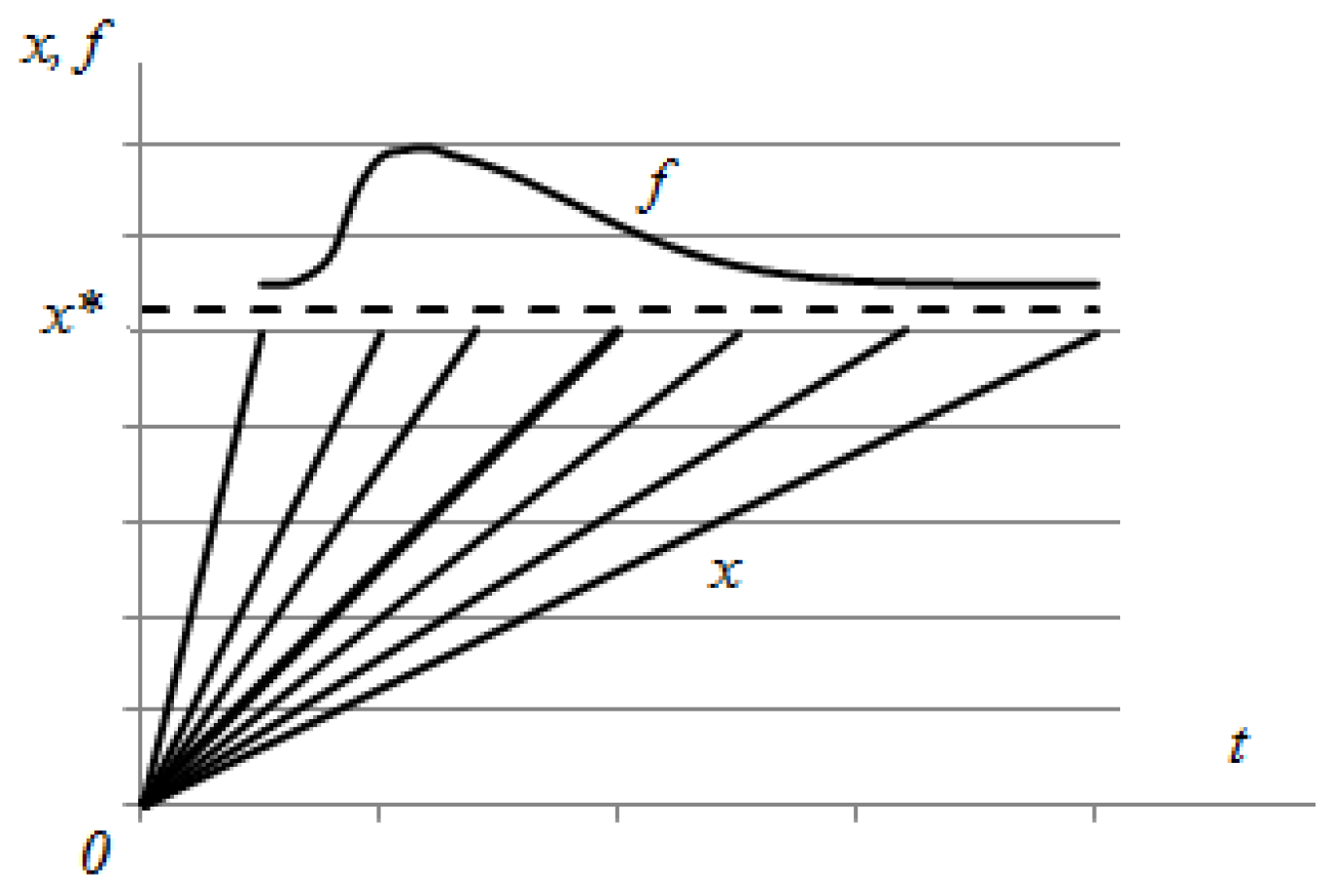
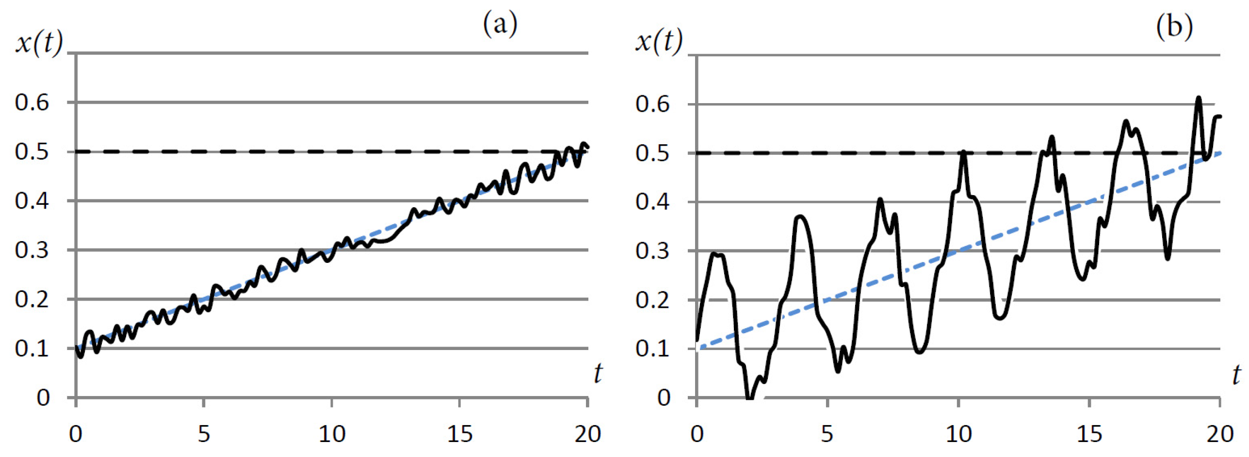
Note that Equation (1) is known in the scientific literature as the stochastic differential equation driven by a Brownian motion. The KP is considered as a random process, and its value at the initial moment of time is determined using the distribution law function . We can assume that there is an increase in KP in the process of operation and degradation of ME. KP may have a monotonic character (the absorbing boundary problem shown in Figure 3a), or non-monotonic character (the transparent boundary problem shown in Figure 3b) [15,21].
Figure 3.
Example of dependency realization of KP on time: for the MD distribution law (a); for the ND distribution law (b).
The problem of determining the time when KP reaches the limit value at is reduced to the problem of the upper boundary of the acceptable area of change reached by process (1).
If a Markov process of the diffusion type is defined by a stochastic equation of the form (1), the conditional transition probability density of this process is described by the Fokker–Planck–Kolmogorov equation:
We should note that drift coefficient and the diffusion coefficient depend only on time and do not depend on .
These types of coefficients, and , do not allow us to take into account the heterogeneity of the structure of modern materials, which were used to manufacture ME. Currently, composite materials and additive technologies are used, with the help of which components and assemblies with a high level of heterogeneity are created. Therefore, it seems promising to construct the mathematical model with coefficients depending both on time and on .
The distribution laws and models discussed above do not allow us to take into account the processes of degradation and aging of modern and advanced ME. The distribution laws and models discussed above do not explicitly take into account the chemical processes occurring in the nodes and elements of the ME and leading to the degradation and aging of the ME. Therefore, it seems promising to construct the mathematical model which permits us to take into account the chemical processes occurring in the nodes and elements of the ME.
Thus, the research works [5,15] analyzed together above with methods [21,22,23] serve as the basis (starting point) for the research outlined in this article.
3. Statement of the Research Problem
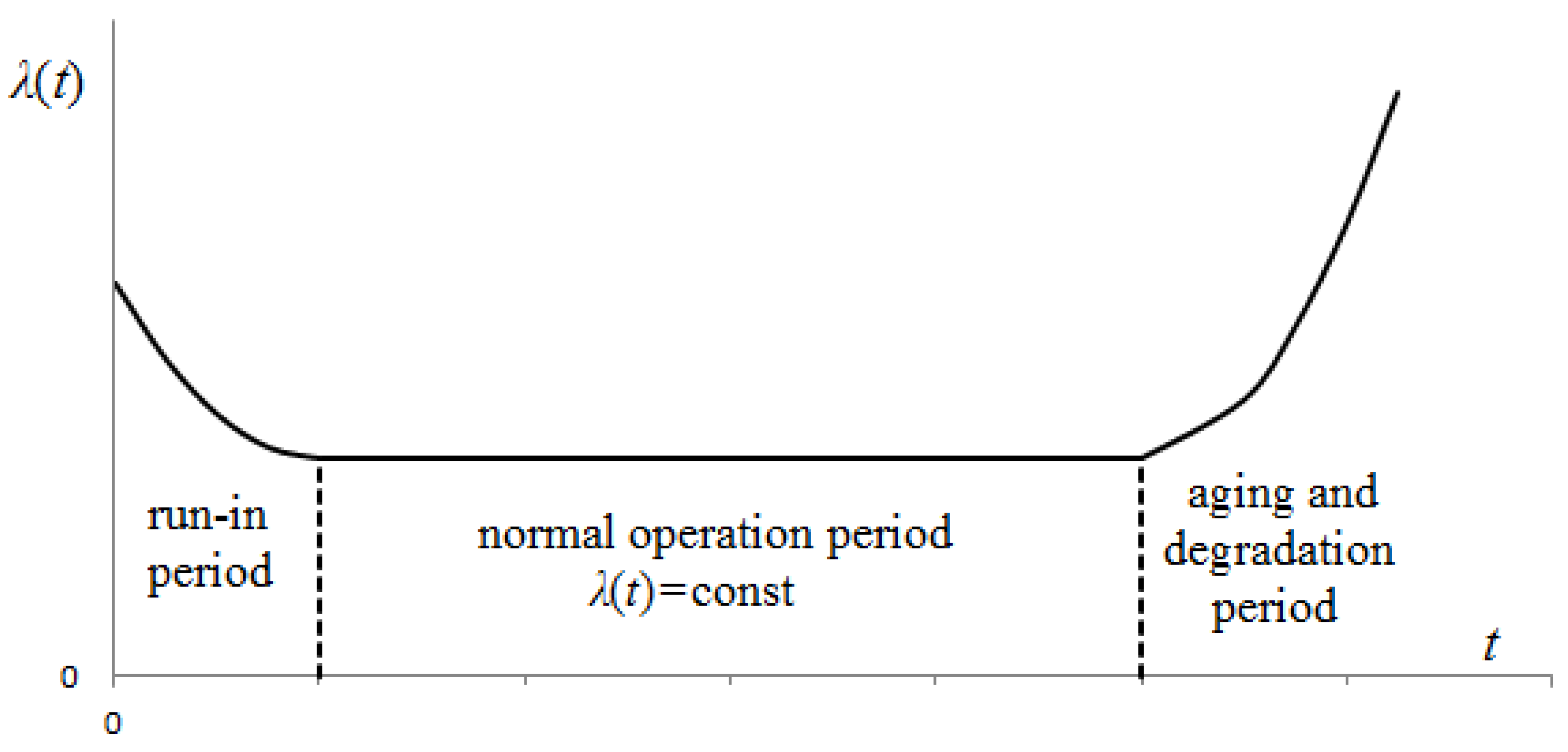
It is required to construct a probabilistic model of degradation and failures, whose parameters have a correct physical meaning. The model should make it possible to simulate the degradation and aging processes of modern and advanced ME made of heterogeneous materials (due to the dependence of coefficients and both on time and on KP ). The model should take into account basic physical and chemical regularities underlying degradation processes (aging processes of ME nodes and elements) leading to failure. In particular, the developed model must adequately describe the function of failure rate , which has a classical U-shaped standard form, presented in Figure 4.
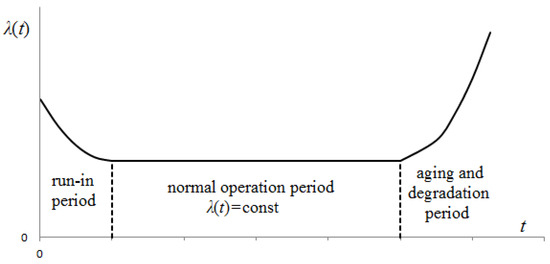
Figure 4.
A standard form of the failure rate function.
According to Figure 4, the operation time is conventionally divided into three characteristic periods: the period of run-in, the period of normal operation and the period of degradation and aging.
The parameters of the developed model should allow us to vary the moments of transition from the run-in period to the normal operation period and further to the period of intensive aging and degradation.
The above problem is the key problem of arranging the metrological support of the ME fleet, which usually consists of several hundred types of ME, having different age, different periods of operation, different levels of aging and degradation. The developed method is to set rational intervals between ME verifications for different groups of ME, which will ultimately improve the target performance of special facilities, in which ME are installed, and increase the effectiveness of their use for the intended purpose.
4. Materials and Methods
4.1. Rationale and Main Assumptions
Analyzing a variety of degradation processes, we can find out that all of them have a random nature, and a change in their indicators has both monotonic and non-monotonic character. Complex mechanical electronic devices, such as integrated circuits and mechatronic systems, are simultaneously subject to the effect of many processes.
The physical nature of the KP of degradation processes under study, which can cause the failure of any component, for example, the component of an integrated circuit, may be different, and it encompasses dislocation accumulation, plastic deformation, fatigue mechanical failure, electromigration, accumulation of voids, generation and movement of charges on the crystal surface of a semiconductor), etc.
The operability of each component of ME is characterized by its functional parameter , . According to the technical documentation, the condition is fulfilled in the operable state, and the failure occurs at or . Here, is given lower limit value of functional parameter, and is given upper limit value of functional parameter. In the general case, is a random function of time, and also depends on the application temperature of ME, and the magnetic load on ME, gravitational and force action on ME, etc.
To obtain a reliable prediction of degradation and failure, it is necessary to have a quantitative model of reliability in the form of dependence of functional parameter on temperature, electrical and magnetic load, gravitational and force impact, etc. Such a model is based on the study of behavior of each functional parameter not only at the moment of failure, but also in the process of its change, i.e., on kinetics of failures. The specified model can be constructed by means of complex accounting of probabilistic-statistical and physico-chemical factors.
Assume that the functional parameters are independent, and the failure of at least one of the parameters leads to the failure of ME as a whole. In this article, we consider one generalized functional parameter , which we will call KP. Since is a random process, the conditional probability density of the distribution of the KP at moment is of interest for practical use.
Assume that the direction of change in the functional parameter and the rate of change at each moment of time is determined only by the loads and influences acting, as well as by the properties of the material of which the “key component” of the ME is made. It is assumed that changes in the magnitude and its rate do not depend on the previous state. Then, the behavior of KP can be approximated by a Markov process of the diffusion type.
Note that many researchers describe the degradation and aging process using the random Markov process (see, for example, [5,15]).
4.2. Diffusion Models of the General Form
Let the drift and diffusion coefficients depend on both time and KP : , . Then, for the Markov process of the diffusion type, conventional transition density is described by the Fokker–Planck–Kolmogorov equation, which is a second-order partial differential equation [15,21]:
It is assumed that a drift in KP is triggered by the effect of physical and chemical processes (oxidation, electrolytic corrosion, etc.) occurring in elements and units of ME during operation. In model (2), this effect is implemented using coefficients and . If drift and diffusion coefficients are set in the general form (depend on both and ), then Equation (2) can only be solved numerically. The analytical solution can be obtained only in some particular cases. This paper focuses on particular cases of analytical solution (2) under the assumption that ME degradation occurs due to chemical processes described by the chemical kinetics equation.
First, we describe some methods of the theory of chemical kinetics, and then we describe some cases of analytical solution of Equation (2).
4.3. Methods of Theory of Chemical Kinetics
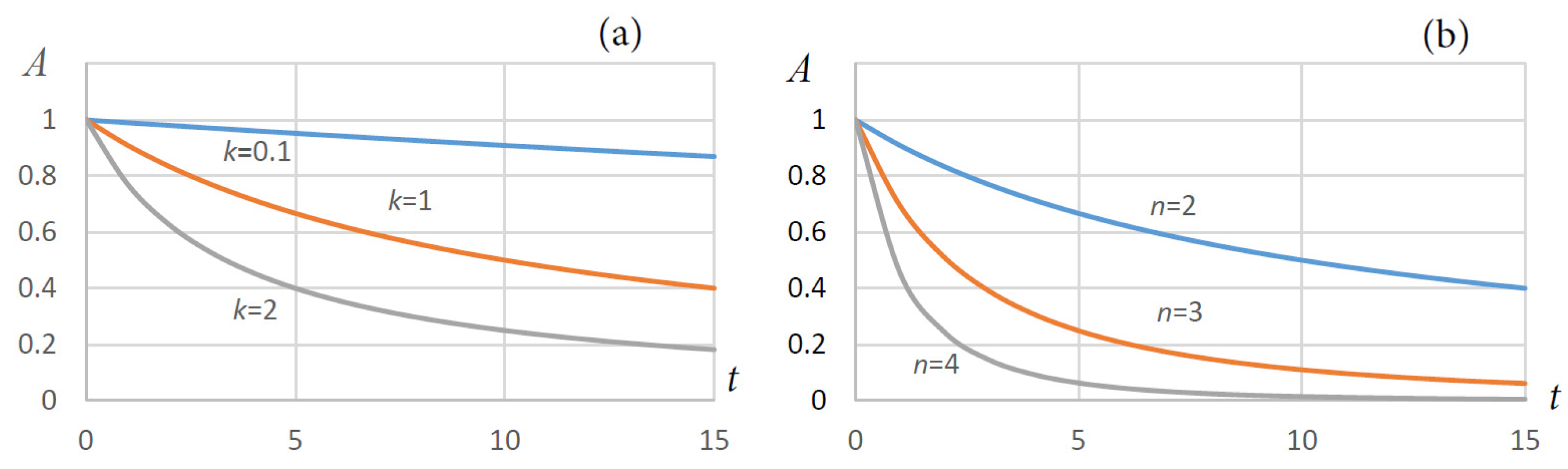
According to the law of Guldberg and Waage [22,23,24], the chemical reaction rate of the i-th reacting substance is proportional to the product of current concentrations of reacting substances:
where is the reaction time, is the reaction rate constant and is the chemical reaction order based on the i-th component (the stoichiometric coefficient of the i-th component).
Differential equations of chemical kinetics for some simple types of chemical reactions are presented in the second column of Table 1.

Table 1.
Some types of equations of chemical kinetics and their solutions.
All equations, presented in the second column of Table 1, can be written as follows:
If function is sufficiently smooth in some domain of its arguments, then, in the case of the following initial condition according to the Cauchy–Lipschitz–Horowitz theorem [22,23,24], there is a single solution to each of the equations presented in the second column of Table 1. These solutions are provided in the third column of Table 1.
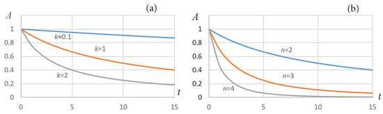
Figure 5.
Dependence of concentration of reacting substances on time: for different values of the rate of chemical reaction (a); for different values of the order of chemical reaction (b).
We can see that concentration decreases if the reaction order and the rate of reaction increase.
4.4. Development and Investigation of a Probabilistic Physico-Chemical Model
4.4.1. The Case of Constant Drift and Diffusion Coefficients, ND Distribution and MD Distribution
Let us consider particular values of coefficients of Equation (2). At first, and , where and are constant. This case corresponds to the chemical reaction for which the constant reaction rate can be assumed to be equal to zero (concentrations of reacting substances remain practically unchanged).
Then, a partial differential equation with constant coefficients follows from (2):
When solving (4), one should set the boundary conditions that depend on the type of random process, in particular, on its monotonic or non-monotonic nature. The initial condition can be set either by means of the -function at point , : , or by means of the distribution function of KP at the initial moment of time. It is also necessary to set the boundary conditions: for non-monotonic distribution: , ; for monotonic distribution: , . The first condition is purely formal since KP cannot take negative values.
The degradation of electronic assemblies and ME components is described by non-monotonic distribution, while the degradation of mechanical assemblies and ME elements is described by monotonic distribution [15].
After finding function that satisfies the preset initial conditions, the function of the probability density of time to boundary and the function of time before failure can be calculated using the following formulas:
Hence, to determine the probability density function of random variable of time before failure, it is necessary to obtain the expression for by solving Equation (4) having appropriate initial and boundary conditions. Further, it is necessary to find the partial derivative of function with respect to time and integrate the obtained expression with respect to parameter . To construct function , it is necessary to integrate function within the appropriate limits. The failure rate is calculated using the following formula: .
Equation (4) can be integrated analytically. The distribution function for the MD distribution law is as follows [15]:
where is the shear coefficient, and is the process variation coefficient.
The distribution function for the ND distribution law is as follows [15]:
Explicit expressions, describing the failure rate for the MD distribution and the ND distribution, are provided in [15]. Hence, distribution densities f(t), distribution functions F(t) and failure rates λ(t) are calculated using finite analytic formulas and normal normalized law distribution (see Section 2.1).
It is necessary to know parameters and to use MD distributions and ND distributions to solve applied problems (for example, to make a reliability evaluation of an ME fleet, to predict the -percent resource of error-free running time, etc.). Formulas needed to perform statistical evaluations of parameters and , using processed testing results for the MD distribution and the ND distribution, are provided in [15].
It can be stated that the MD distribution and the ND distribution are two-parameter distributions. However, two parameters and cannot ensure sufficient accuracy and adequacy of the model in terms of, for example, the following three values simultaneously: mathematical expectation, mean square deviation and —percent operating time before failure ((100-)—percent resource) (it should be —percent resource). Therefore, we will consider distributions depending on a larger number of parameters.
4.4.2. Methods of Solving Equation (2) in the Case of Variable Drift and Diffusion Coefficients
Let us suppose the following:
- (A)
- Drift coefficient is linearly dependent on KP:, where , —are functions of time;
- (B)
- Function is proportional to concentration : , where is a constant value.
- (C)
- Diffusion coefficient depends on time only (it does not depend on ): .
We introduce new variables to solve stochastic Equation (2) according to [21]:
Then, conventional probability density can be written as follows:
where is the new KP distribution density function. By selecting functions and , we can determine coefficients and , so that we can find an analytic expression for from Equation (2) after switching to new variables (8).
Then, Equation (2) can be represented as the simplest parabolic equation:
Equation (9) should be solved for pre-set initial and boundary conditions. It is noteworthy that the form of solution (9) will strongly depend on specific initial and boundary conditions.
4.4.3. Solution of Equation (9) If Initial and Boundary Conditions Are Set as -Functions
If initial and boundary conditions are set as the -function at point and , . Then, solution (9) is as follows [17,21]:
If variables and can be expressed as finite formulas by applying and to Formula (8), then Equation (2) can be solved analytically. Let us consider the cases of analytic solution (2).
Case 1. Let us assume that , ; and are constant for a chemical reaction of order 2: . Then
Then, analytic expressions for functions and are as follows:
and partial derivative is written as . Hence, finite formulas are obtained for function in Case 1.
Case 2. , , ; where and are constant. Then:
Case 3. , , . Then
Case 4. , , . Then
Case 5. , , . Then
We also obtained finite formulas for function in cases 2–5.
Case 6. , , . Then and the integral can be calculated using numerical method. Explicit expressions in the form of infinite sums are not provided for this integral due to cumbersome formulas.
It is known from [2,19] that the probability density of the time needed for KP to reach its maximum acceptable value is calculated using Formula (5).
The model, described in Section 4.4.3, has boundary and initial conditions at point . Therefore, it is reasonable to use this model to simulate the KP drift process, when ME undergoes strict production control at a production enterprise, and KP variability is minimal at the time when the product manufacturing process is completed.
4.4.4. Method of Calculating the Probability of KP Reaching Limit Values for the First Time
The equation for the probability of KP reaching limit values for the first time is as follows [21,25]:
where is the given initial value of KP. Equation (11) should be solved with the initial condition , boundary conditions and ( is given lower limit value of KP, is given an upper limit value of KP) and the additional condition .
4.4.5. Method of Calculating the Average Time Needed for KP to Reach Limit Values for the First Time
The equation for calculating the average time needed for KP to reach limit values for the first time, when coefficients and do not depend on time, is as follows [21,25]:
Here, is the given initial value of KP. Equation (12) can be solved analytically. The solution is as follows:
The equation for calculating the average time needed for KP to reach its limit values for the first time, when coefficients and depend on time, can only be solved numerically. The equations for calculating the average time needed for KP to reach its limit values for the second and third times have a more complex iterative form [21,25].
4.4.6. Method of Solving Equation (9) If Initial and Boundary Conditions Are Set in the General Form
If initial and boundary conditions are set in the general form for Equation (9), the problem will be formulated in the same way as the classical problem of heat propagation in an infinite rod, whose lateral surface is thermally insulated [14]:
with initial condition:
where is time, is the current coordinate of the rod cross section, is temperature at the moment of time in the rod cross section with coordinate , , is the heat conductivity coefficient, is the heat capacity of the material and is density of the rod material.
The general solution to the heat conductivity problem (14)–(15) is represented as the Poisson integral [14]:
We show that the problems (9) and (10) can be obtained as a special case using problems (14)–(16). If we make a substitution in (14), (, , , ), we obtain Equation (9).
Let us set as a -function at point . Then, if we make the same substitution and set as a -function at point in (16), we obtain expression (10) from (16).
It is reasonable to use a model with general boundary conditions to simulate the KP drift process in the case when some variability of KP is acceptable for products manufactured at a production enterprise, and this KP can be described using distribution function . As a rule, is truncated normal distribution with mathematical expectation, which does not exceed a certain value of , and a sufficiently small value of the mean square deviation.
4.5. Method of Parameterization of a Probabilistic Physico-Chemical Model Based on Statistical Information Processing
This probabilistic physico-chemical model (more specifically, the drift coefficient function) has 5 parameters: , , , , . They allow for a more precise fine-tuning of the model based on the results of statistical data processing. In particular, model parameters can be chosen in the way that ensures the best approximation in terms of such parameters as mathematical expectation, mean square deviation and time before failure, in comparison with diffusion monotonic and non-monotonic models (with the number of parameters equaling 2).
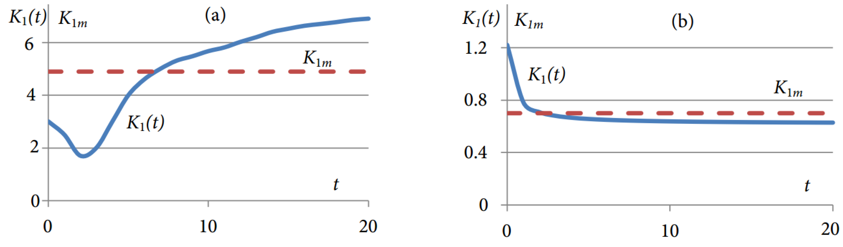
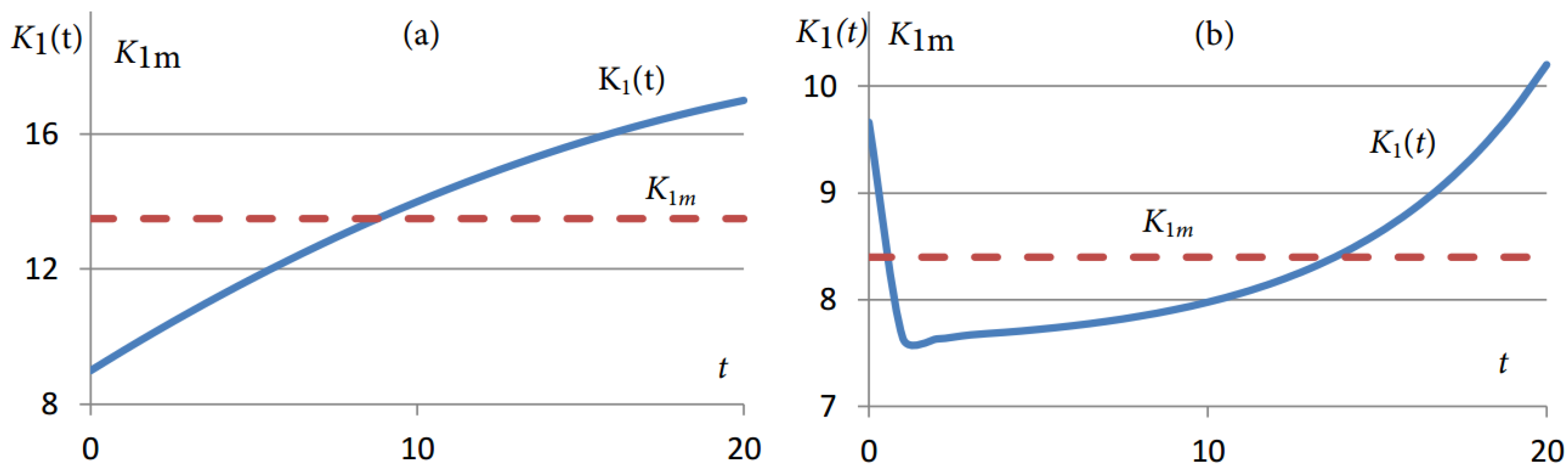
The drift coefficient is as follows: . Taking into account the equation of chemical kinetics, the form of function is determined by the order of reaction and rate constant , and it also depends on initial concentration . The analysis has shown that by varying each of and parameters, we can greatly influence the form of function . For example, we can obtain such a form of function , so that coefficient values were smaller at the initial period of KP change (increasing function K1(t)) shown in Figure 6a and Figure 7a, or at the final period of KP change (decreasing function K1(t)) shown in Figure 6b and Figure 7b. The red line shows mean values of coefficient in Figure 6a,b and Figure 7a,b.
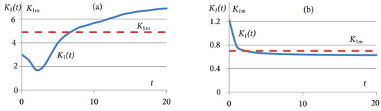
Figure 6.
Variability of the reaction rate coefficient: k = 0.8 (a); k = 3 (b).
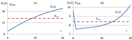
Figure 7.
Variability of the reaction order: n = 1.5 (a); n = 3 (b).
Hence, in the time interval , the same mean value of coefficient can be obtained both for increasing function , and for decreasing function . According to the Lagrange theorem about the mean value of a function in the interval, darkened areas of curvilinear trapezoids, located above the straight line and below the straight line will be equal in value.
Due to the changeability of parameters, that have a clear physical and chemical origin, the variability of coefficients and allows for a more precise fine-tuning of the model according to the results of statistical data processing.
5. Results
5.1. The Results of Studying the Model and Its Components
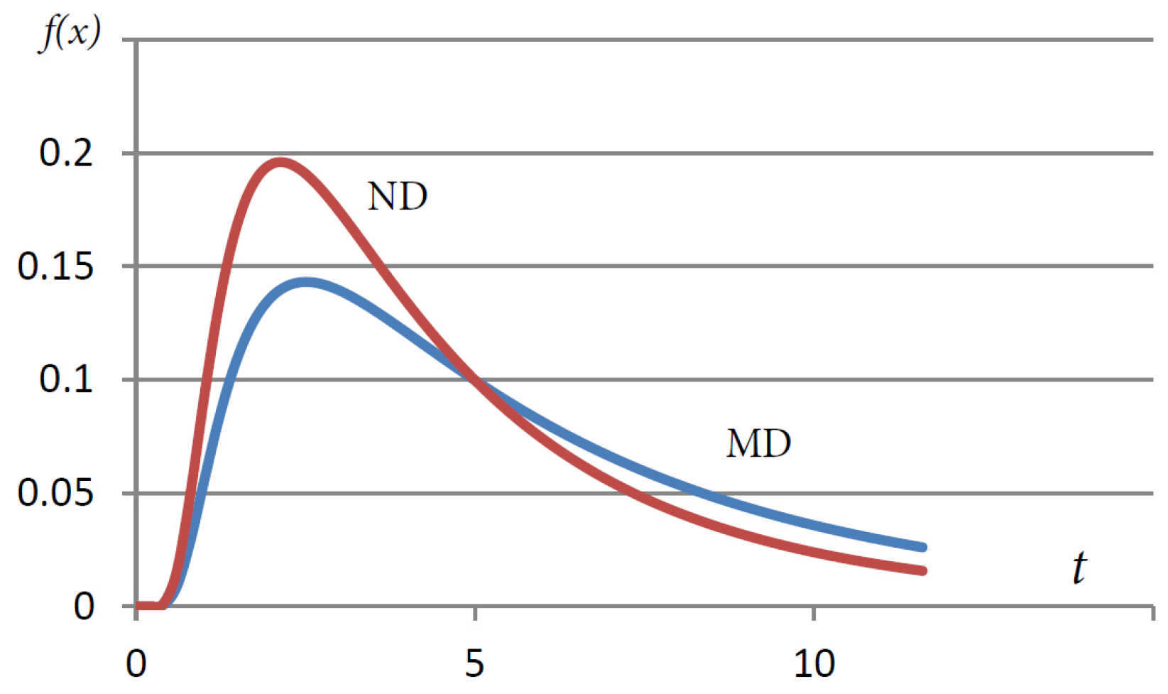
A standard graphical representation of distribution density function f(t) for MD distribution and ND distribution is shown in Figure 8.
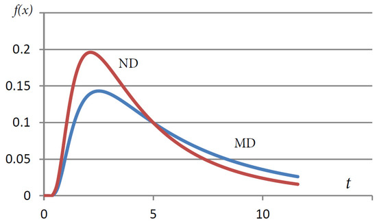
Figure 8.
MD distribution and ND distribution.
It is noteworthy that the MD distribution coincides with the Birnbaum–Saunders distribution [26] to the accuracy of the nearest constant.
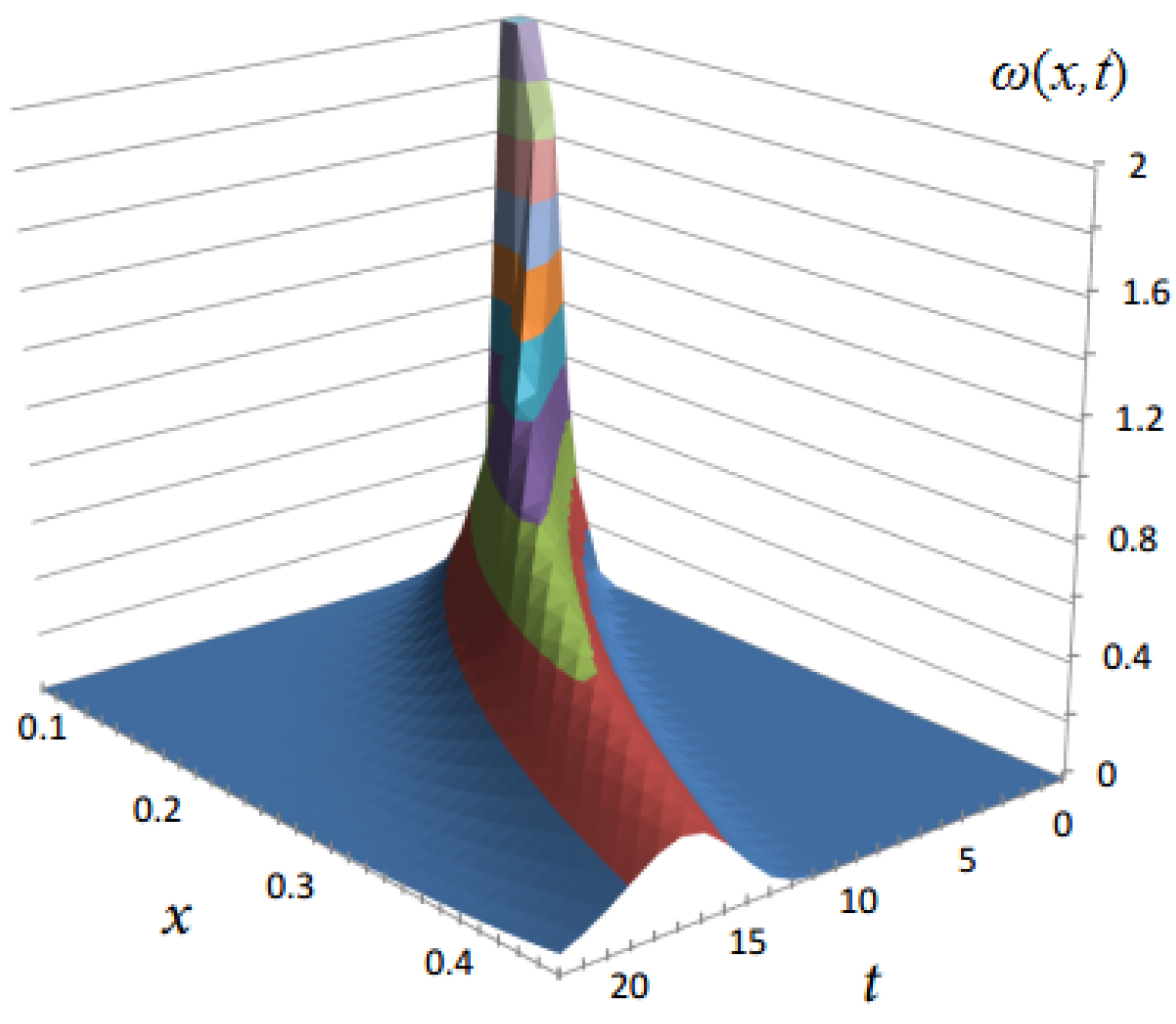
The two-dimensional surface of conventional probability density function at , , , is shown in Figure 9. Initial and boundary conditions were set using the -function at point , .

Figure 9.
The surface of conventional probability density function for the 2nd order reaction when initial and boundary conditions are set using -function.
Since the limit value is , then, for clarity purposes, the part of the surface, extending to infinity, is chipped off by plane .
The characteristic time of application is years for the class of ME considered in this paper. KP increases by 3–6 times in the process of ME degradation. As a result of the analysis of surface cross section plots, we find that a great change in KP in the first half of the time interval is most probable.
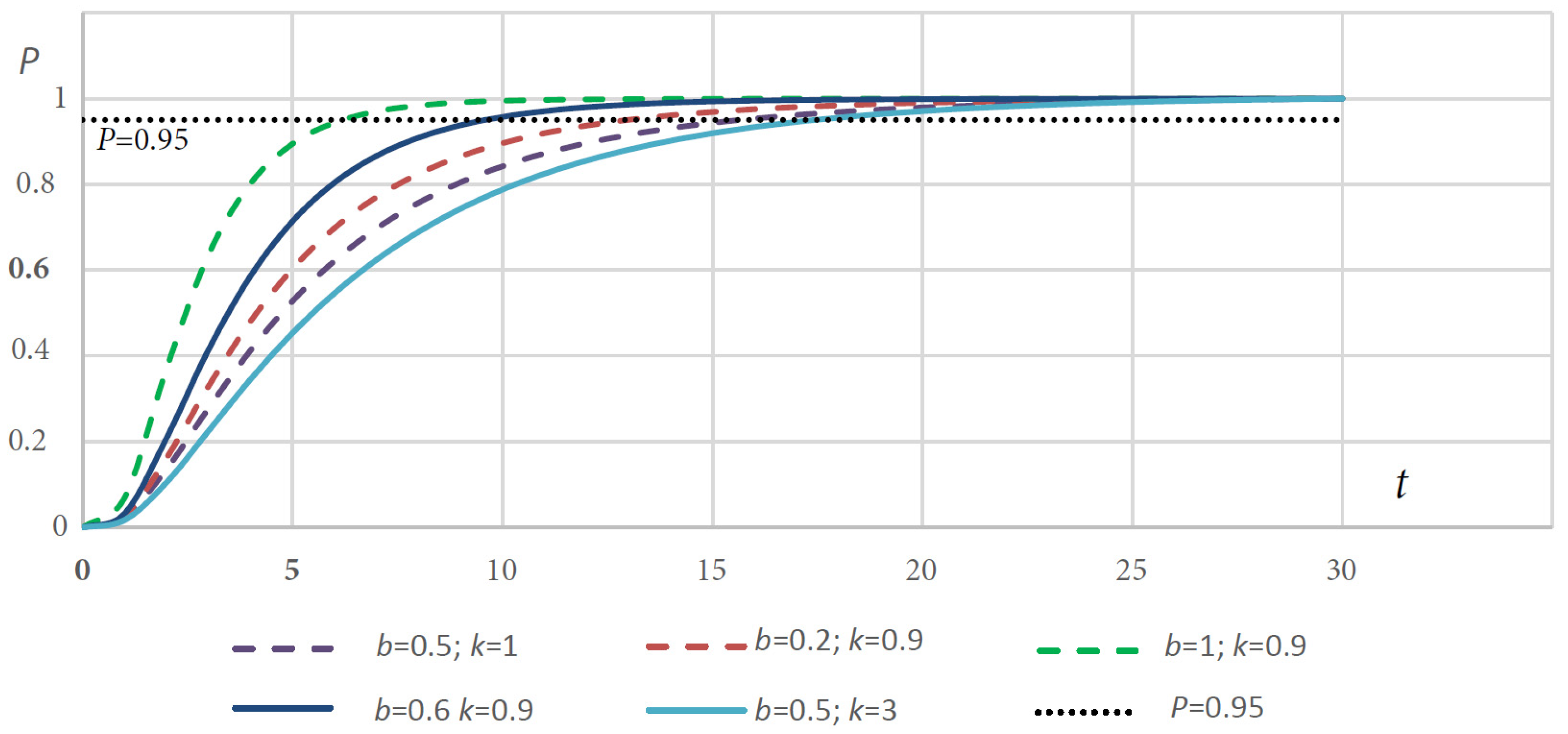
Dependences between probability P of reaching the KP limit value and the operation time for different values of parameters and (at , ) are shown in Figure 10. The dotted line shows confidence probability P = 0.95. It is clear that an increase in parameter (at ) reduces the time to the confidence domain. The increasing parameter (at ; ) increases the time to the confidence domain.
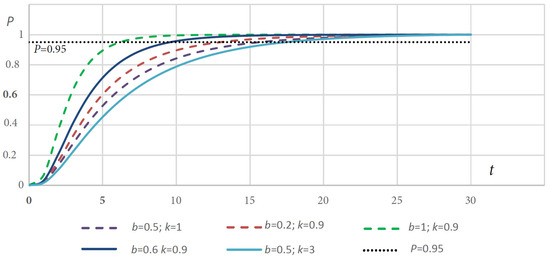
Figure 10.
Dependence between probability P and operation time for different values of parameters and .
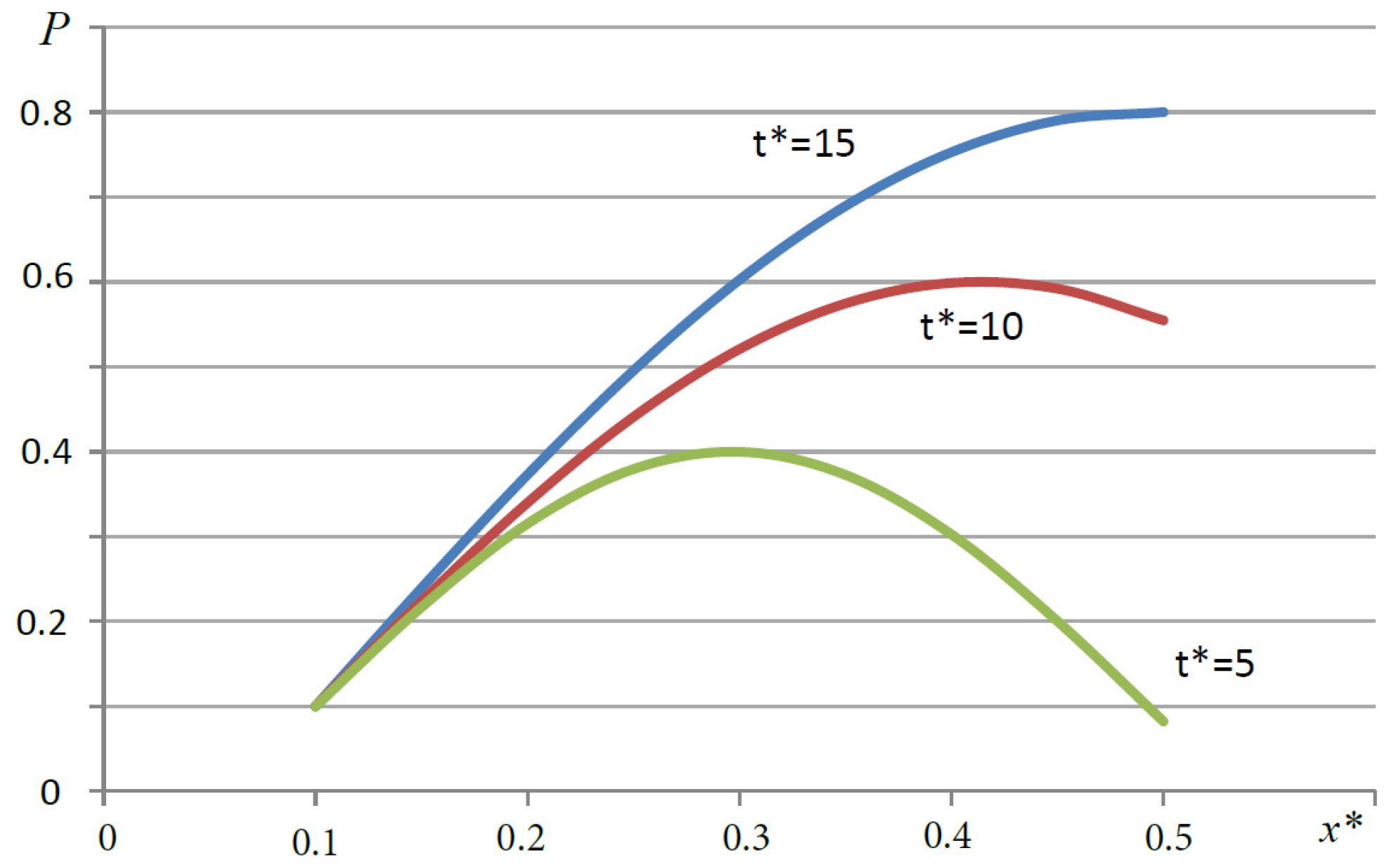
Dependence between probability P of reaching the KP limit value on limit value for different values of is shown in Figure 11.
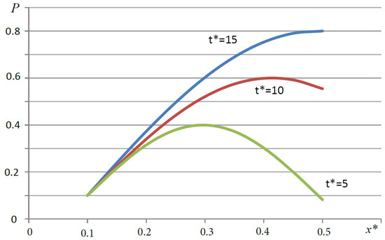
Figure 11.
Dependence between probability P and limit value at different values of .
It can be seen that the probability of reaching limit value increases with increasing .
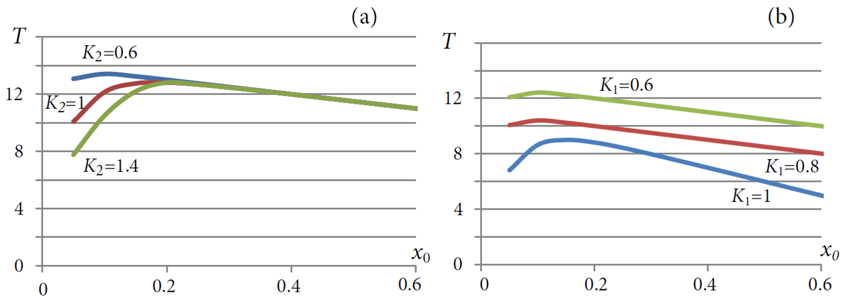
The dependence of mean time T, needed for KP to reach its limit value , on initial value , for and for different values of , is shown in Figure 12a. The case of and different values of is shown in Figure 12b.
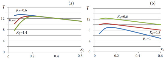
Figure 12.
Dependence of the mean time, needed for KP to reach the limit value , on value for different values of the diffusion coefficient (a); for different values of the drift coefficient (b).
We can see that as increases, the mean time reduces. As the drift coefficient increases, the mean time reduces. As the diffusion coefficient increases, the mean time increases.
If initial and boundary conditions are set in the general form, the two-dimensional surface of conventional probability density function is as shown in Figure 13.
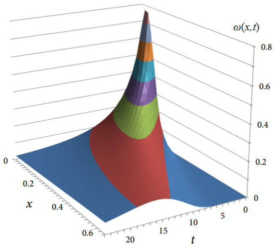
Figure 13.
The surface of conventional probability density function for the 2nd order reaction at .
It can be seen that function is limited from above and does not extend to infinity as the function shown in Figure 9.
5.2. The Results of Applying the Probabilistic Physico-Chemical Model to a Practical Problem
Now we describe the results of applying the model, developed in this article, to the problem of constructing the function of the failure rate. This task is one of the most important ones for the design companies involved in the design of new promising ME specimens, as well as the companies involved in the modernization of existing ME specimens.
The failure rate function can be calculated using the formula:
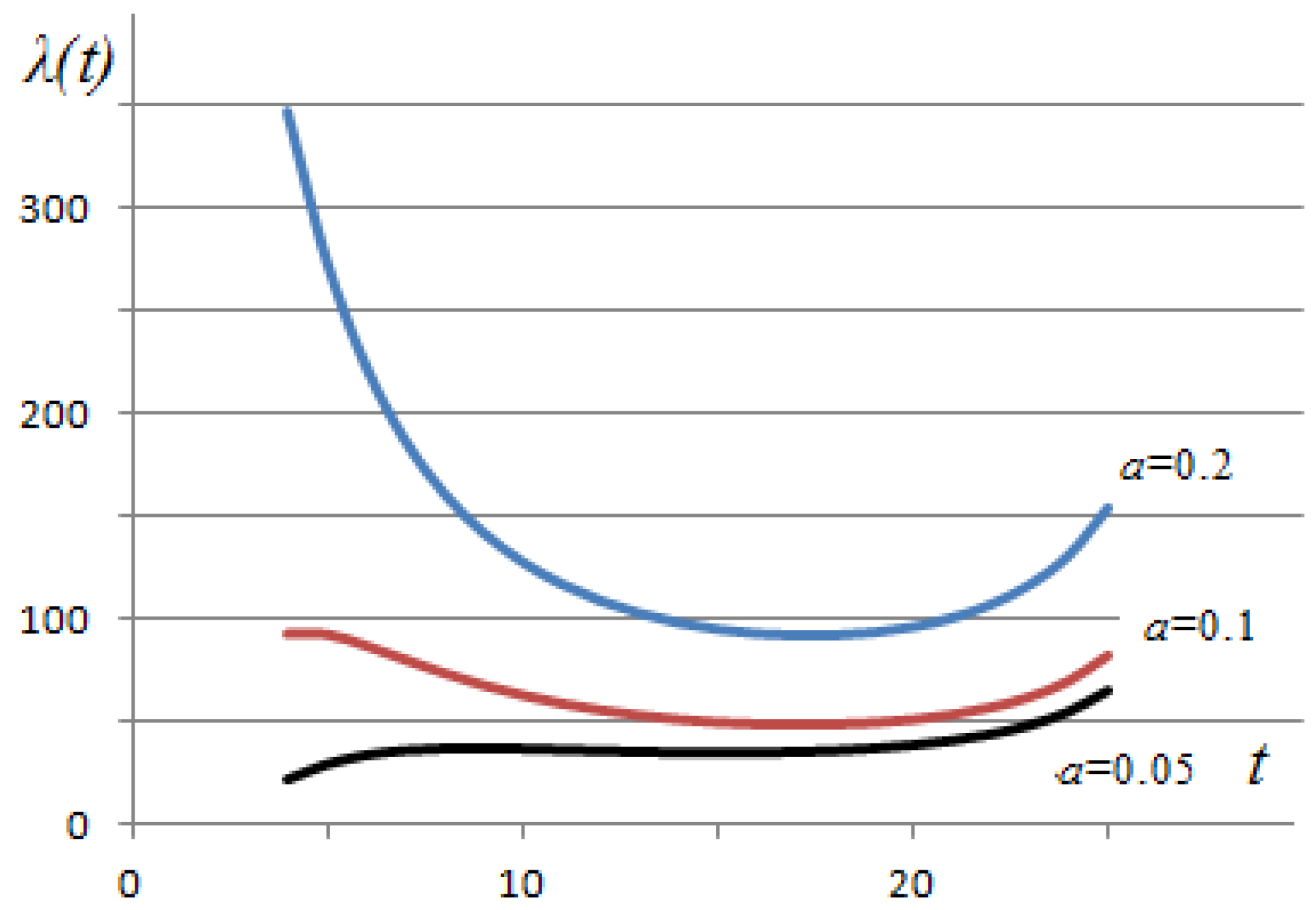
Figure 14 shows the standard form of function at and different values of the initial concentration of the reactants.

Figure 14.
Dependence of the failure rate on time at different values of initial concentration .
It can be seen that as the initial concentration decreases, the average failure rate decreases. By changing the initial concentration of the reactants, the failure rate can be reduced from 90 to 40 [units/year] during the normal operation period.
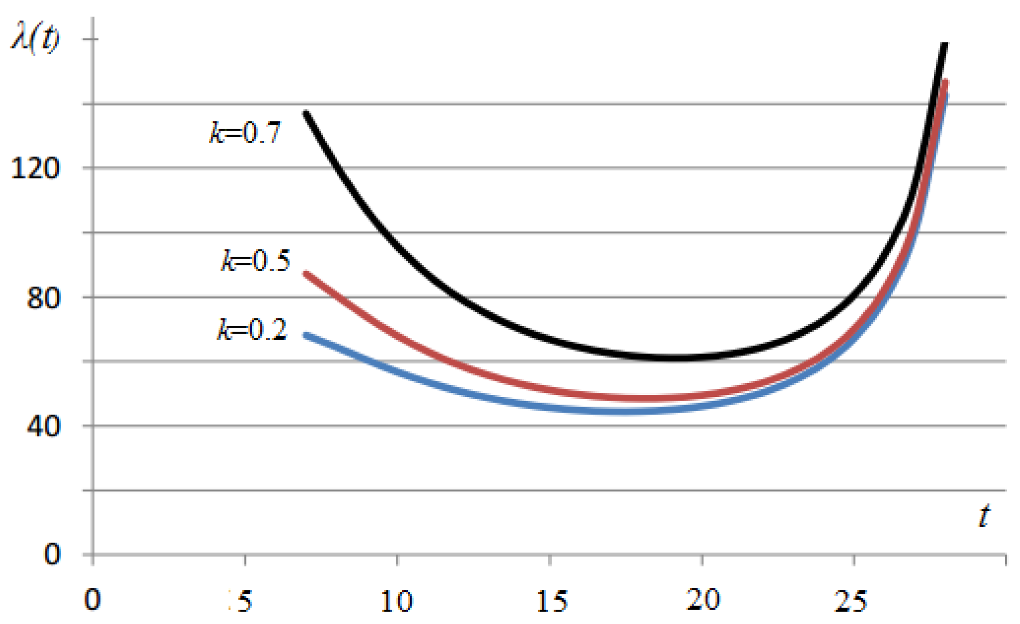
Figure 15 shows the standard form of function at and different values of the chemical reaction rate .
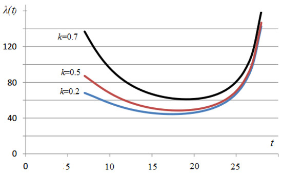
Figure 15.
Dependence of the failure rate on time at different values of the chemical reaction rate .
We can see that the average failure rate decreases as the chemical reaction rate decreases. By changing the chemical reaction rate, the failure rate can be reduced from 65 to 47 [units/year] during the normal operation period.
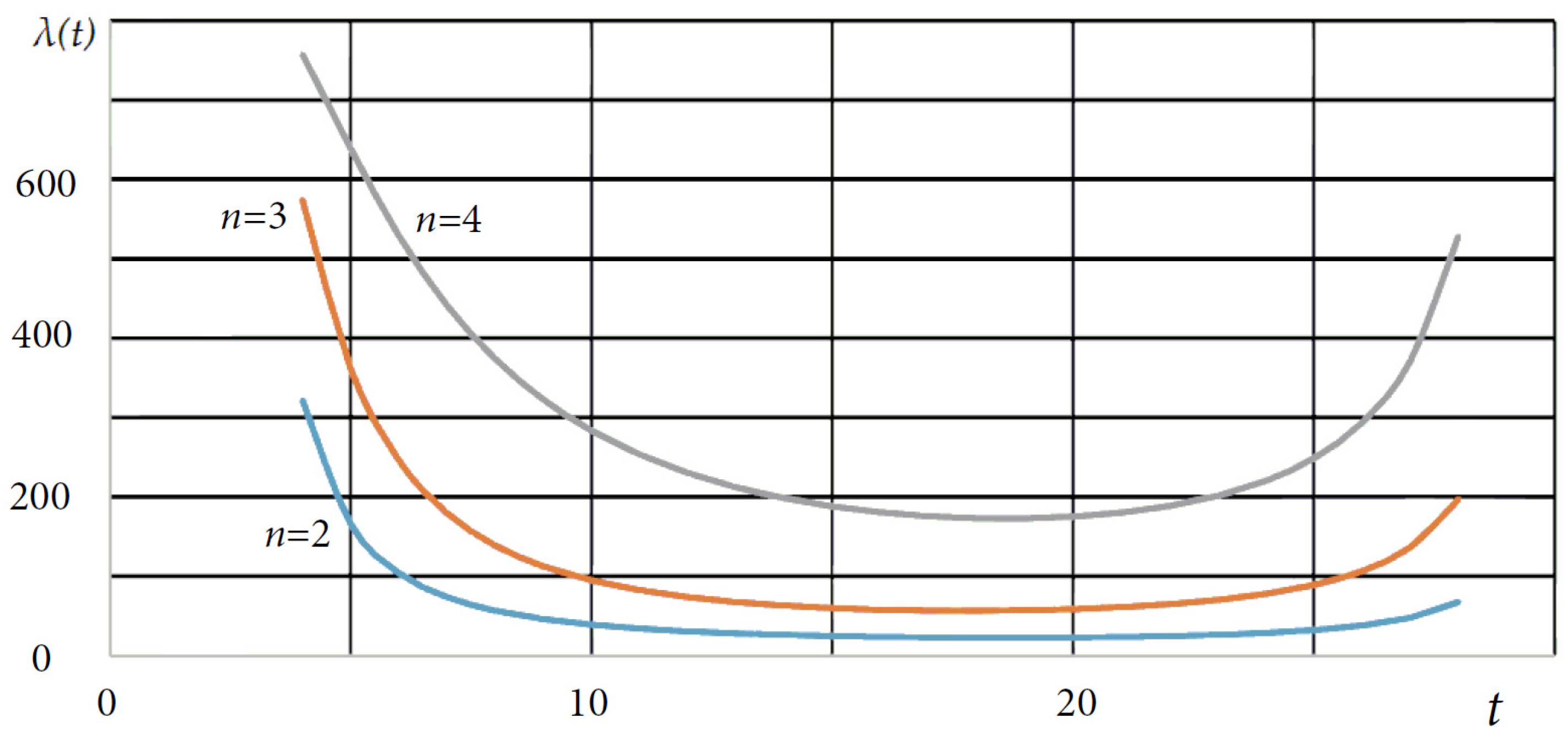
Figure 16 shows the standard form of function at and different values of the chemical reaction order .
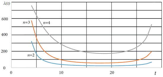
Figure 16.
Dependence of failure rate on time at different values of the chemical reaction order .
It can be seen that as the chemical reaction order decreases, the average failure rate decreases. By changing the chemical reaction order, the failure rate can be reduced from 170 to 20 [units/year] during the normal operation period.
Thus, by varying parameters , and , it is possible to significantly (several times) reduce the ME failure rate during the period of normal operation. It should also be noted that by varying these parameters, it is possible to change the time of transition from period of normal operation to period of aging and degradation. However, recent changes are not as significant as changes in the failure rate value at the period of normal operation.
In practice, a specially developed set of Compliance Tables is used in the design of the ME. First, based on the goals and objectives of the design, the tactical and technical requirements for the designed ME are determined. Based on the tactical and technical requirements, based on the use of the developed model, the rate and order of the chemical reaction are determined, as well as the concentrations of reacting substances that provide the required tactical and technical requirements. Further, according to the rate of chemical reaction, the order of chemical reaction and the concentration of reacting substances, materials and technologies for the production of ME components and assemblies are determined.
6. Discussions
Table 2 shows the results of comparison between the MD model [15], the ND model [15], the diffusion probabilistic physical model [19] and the probabilistic physico-chemical diffusion model.
Table 2.
Comparison of models by the number of parameters.
Comparable models have from 2 to 5 parameters, which in some cases can be estimated using the results of statistical information processing based on the analysis of performance and reliability of operation of similar ME specimens. In the absence of statistical information (for example, during the development of new promising specimens of ME) the model, presented in this article, is the only unique instrument that can be used to prognosticate their reliability and serviceability.
As noted above, MD distribution is used to simulate mechanical assemblies and ME components, and ND distribution is used to simulate electronic components and ME units. A diffusion probabilistic physical model [19] is used to simulate the metrological characteristics of ME.
The probabilistic physico-chemical diffusion model, presented in this article, has five parameters. Three of them, , and , have a clear physico-chemical origin: is the rate of chemical reaction and is the order of chemical reaction, is the concentration of the reagent at the initial moment of time.
It is noteworthy that parameters , and allow the simulation of different production technologies and materials used in the mass production of ME units and elements. So, for example, parameter is responsible for different levels of perfection of technologies as a whole (for example, advanced technologies, modern technologies or obsolete technologies). Parameter is responsible for the chemical catalysts and additives used, which affect the rate of the chemical reaction. Parameter is responsible for the choice of specific production materials (it allows for material properties to be taken into account) used to produce ME assemblies and elements.
The model, developed by the author, can help to identify the weakest nodes, links and components of ME, due to which ME becomes inoperable, and to provide recommendations on the use of production materials whose physical and chemical properties are most suitable for the manufacture of particular nodes and components.
Therefore, the probabilistic physico-chemical diffusion model, presented in this article, is preferable, because it can adequately simulate the U-shape of the failure rate function. All other models considered and analyzed in this article are helpless here.
7. Conclusions
The new probabilistic physico-chemical diffusion model of the key drifting parameter of ME (the model of degradation and failures) is developed. The model is based on the combined application of the Fokker–Planck–Kolmogorov equation and the chemical kinetics equation. The parameters of the model have a proper physical and chemical meaning. The model takes into account basic physical and chemical regularities underlying degradation processes (aging processes of ME nodes and elements) leading to the failure state.
An analytical solution to the Fokker–Planck–Kolmogorov equation was constructed for several types of chemical kinetics equations.
The model allows the compilation and analysis of a wide range of reliability indicators and metrological characteristics [27] and to make predictions about their behavior.
The model adequately describes the function of the failure rate, which has a classical U-shape. Neither reliability and degradation model, known to the author, allows the acquisition of three periods: the run-in period, the period of normal operation and the aging and degradation period within one model.
The presented method allows us to establish rational periods between ME verifications and calibrations for different groups of ME, which ultimately increase the target performance of special facilities, where ME are installed, and raise the effectiveness of their use for their intended purpose.
The model is used to accomplish the tasks of forecasting, to establish rational periods between ME verifications and calibrations, and to simulate the indicators of reliability of ME as a whole, as well as its soldered joints and modern integrated circuits used as part of special equipment and machinery [27] which may be operated under harsh conditions and in corrosive environments.
Funding
This research received no external funding.
Institutional Review Board Statement
The study was conducted in accordance with the Declaration of Helsinki, and approved by the Institutional Review Board of Moscow State University of Civil Engineering (protocol № 1 5 December 2022).
Data Availability Statement
Data are contained within the article.
Acknowledgments
The author is grateful to Yury Filippovich Golubev, at the Keldysh Institute of Applied Mathematics of Russian Academy of Science, for his comprehensive support of scientific developments and for helpful discussions.
Conflicts of Interest
The author declares no conflicts of interest.
References
- Yan, T.; Lei, Y.; Li, N.; Wang, B.; Wang, W. Degradation modeling and remaining useful life prediction for dependent competing failure processes. Reliab. Eng. Syst. Saf. 2021, 212, 107638. Available online: https://ideas.repec.org/a/eee/reensy/v212y2021ics0951832021001794.html (accessed on 8 March 2023). [CrossRef]
- Jiang, D.; Xie, J.; Cui, W.; Song, B. A mechanical system reliability degradation analysis and remaining life estimation method with the example of an aircraft hatch lock mechanism. Reliab. Eng. Syst. Saf. 2023, 230, 108922. Available online: https://www.researchgate.net/publication/365098134_A_mechanical_system_reliability_degradation_analysis_and_remaining_life_estimation_method--With_the_example_of_an_aircraft_hatch_lock_mechanism (accessed on 8 March 2023). [CrossRef]
- Romero, E.E.; Bérenguer, C.; Martinez, J. Long-term degradation estimation of wind turbine drive-train under a gain-scheduling control strategy according to the weather conditions. IFAC-PapersOnLine 2022, 55, 13–18. Available online: https://www.researchgate.net/publication/363895260_Long-term_degradation_estimation_of_wind_turbine_drive-train_under_a_gain-scheduling_control_strategy_according_to_the_weather_conditions (accessed on 8 March 2023). [CrossRef]
- Verezemsky, V.G. Probabilistic fatigue damage summation hypothesis. Chem. Oil Gas Eng. 2007, 10, 40–44. Available online: https://elibrary.ru/item.asp?id=9580265 (accessed on 8 March 2023). [CrossRef]
- Kordonsky, K.B. Probabilistic Analysis of the Wear Process; Science Press: Moscow, Russia, 1968; 56p, Available online: https://www.studmed.ru/kordonskiy-hb-i-dr-veroyatnostnyy-analiz-processa-iznashivaniya_66cd8e93344.html (accessed on 8 March 2023).
- Emelyanov, V.S.; Rabchun, A.V. Scope of Applicability of Diffusion Distributions in Reliability Problems. At. Energiya 1991, 71, 28–32. Available online: http://elib.biblioatom.ru/text/atomnaya-energiya_t71-1_1991/go,29/ (accessed on 8 March 2023).
- Popenkov, A.Y.; Fufaeva, O.V.; Khayrullin, R.Z. Analysis of operation models of complex technical systems with degrading metrological support. Izvestia of the Tula State University. Tech. Sci. 2022, 7, 247–254. Available online: https://cyberleninka.ru/article/n/analiz-modeley-ekspluatatsii-slozhnyh-tehnicheskih-sistem-s-degradiruyuschim-metrologicheskim-obespecheniem (accessed on 8 March 2023).
- Wei, W.; Wei, X.; Jiankang, L. Stochastic P-bifurcation analysis of a class of nonlinear Markov jump systems under combined harmonic and random excitations. Phys. A Stat. Mech. Appl. 2021, 582, 126246. Available online: https://econpapers.repec.org/article/eeephsmap/v_3a582_3ay_3a2021_3ai_3ac_3as0378437121005197.htm (accessed on 8 March 2023). [CrossRef]
- Neama, S.; Youssef, T. Comparison of fuzzy semi-Markov models for one unit with mixed standby units with and without preventive maintenance using regenerative point method. Heliyon 2021, 7, e07717. Available online: https://www.sciencegate.app/document/10.1016/j.heliyon.2021.e07717 (accessed on 8 March 2023).
- Meshalkin, V.P.; Boyarinov, Y.G. Semi-Markov models of the processes of functioning of complex chemical-technological systems. Theor. Found. Chem. Technol. 2010, 44, 198–204. Available online: https://istina.msu.ru/publications/article/100926190/ (accessed on 8 March 2023).
- Ma, J.; Fouladirad, M.; Grall, A. Flexible wind speed generation model: Markov chain with an embedded diffusion process. Energy 2018, 164, 316–328. Available online: https://www.researchgate.net/publication/327381227_Flexible_wind_speed_generation_model_Markov_chain_with_an_embedded_diffusion_process (accessed on 8 March 2023). [CrossRef]
- Kravchenko, V.F.; Lutsenko, V.I.; Masalov, S.A.; Pustovoit, V.I. Analysis of non-stationary signals and fields using nested semi-Markov processes. Rep. Acad. Sci. 2013, 453, 151–154. Available online: https://istina.msu.ru/publications/article/141899202/ (accessed on 8 March 2023).
- Kuznetsov, S.V. Mathematical models of processes and systems of technical operation of avionics as Markov and semi-Markov processes. Sci. Bull. MSTU GA 2015, 213, 28–33. Available online: https://cyberleninka.ru/article/n/matematicheskie-modeli-protsessov-i-sistem-tehnicheskoy-ekspluatatsii-avioniki-kak-markovskie-i-polumarkovskie-protsessy (accessed on 8 March 2023).
- Aramanovich, I.G.; Levin, V.I. Equations of Mathematical Physics; Science Press: Moscow, Russia, 1969; 288p, Available online: https://www.studmed.ru/aramanovich-ig-levin-vi-uravneniya-matematicheskoy-fiziki_d2ff39b0a8d.html (accessed on 8 March 2023).
- Azarskov, V.N.; Strelnikov, V.P. Reliability of Control Systems and Automation; National Aviation University: Kiev, Ukraine, 2004; 164p, Available online: https://www.studmed.ru/azarskov-vn-strelnikov-vp-nadezhnost-sistem-upravleniya-i-avtomatiki_881a18fe6fa.html (accessed on 8 March 2023).
- Chigarev, A.V.; Borisov, A.V. Limit Loads in Human Joints. Bulletin of ChGPU Named after I. Yakovlev; Series: Mechanics of the Limit State; Chelyabinsk, Russia, 2010; Volume 2, pp. 548–552. Available online: http://limit21.ru/?do=online&vid=2&nom=432 (accessed on 8 March 2023).
- Chigarev, A.V.; Borisov, A.V. Diffusion model of the destruction of elements of the human musculoskeletal system. Russ. J. Biomech. 2012, 16, 22–37. Available online: https://readera.org/diffuzionnaja-model-razrushenija-jelementov-oporno-dvigatelnogo-apparata-146216051 (accessed on 8 March 2023).
- Admakin, A.L. Markov Chains—A Stochastic Model of Analysis Severely Burned Condition. Medico-Biological and Socio-Psychological Problems of Safety in Emergency Situations. 2016, pp. 119–125. Available online: https://mchsros.elpub.ru/jour/article/viewFile/271/273 (accessed on 8 March 2023).
- Khayrullin, R.Z. Diffusion model of drift of metrological characteristics of measuring equipment. Sci. Tech. Bull. Volga Reg. 2022, 12, 79–82. Available online: https://ntvprt.ru/ru/archive-vypuskov (accessed on 8 March 2023).
- Pronikov, A.S. Machine Reliability; Mashinostroenie: Moscow, Russia, 1978; 592p, Available online: https://lib-bkm.ru/load/73-1-0-1422 (accessed on 28 April 2023).
- Kolmogorov, A.N. Analytical methods of probability theory. Adv. Math. Sci. 1938, 5, 283. Available online: https://www.mathnet.ru/php/archive.phtml?wshow=paper&jrnid=rm&paperid=8951&option_lang=rus (accessed on 8 March 2023).
- Trifonov, K.I.; Devisilov, V.A. Physico-Chemical Processes in the Technosphere; FORUM Publishing House: Moscow, Russia, 2020; 256p, Available online: https://znanium.com/catalog/document?id=399375 (accessed on 8 March 2023).
- Cherepanov, V.A.; Aksenova, T.V. Chemical Kinetics; Ural University Press: Ekaterinburg, Russia, 2016; 132p, Available online: https://znanium.com/catalog/document?id=423690 (accessed on 8 March 2023).
- Stromberg, A.G. Physical Chemistry. In Textbook for Chem. Specialist. Universities; High School Press: Moscow, Russia, 2003; 527p, Available online: https://www.studmed.ru/stromberg-a-g-semchenko-d-p-fizicheskaya-himiya_2aa53f3c14c.html (accessed on 8 March 2023).
- Kazakov, V.A. Introduction to the Theory of Markov Processes and Some Radio Engineering Problems; Soviet Radio Press: Moscow, Russia, 1973; 232p, Available online: https://libarch.nmu.org.ua/handle/GenofondUA/41948?show=full (accessed on 8 March 2023).
- Birnbaum, Z.W.; Saunders, S.C. A New Family of Life Distribution; Cambridge University Press: Cambridge, UK, 2016; Available online: https://www.cambridge.org/core/journals/journal-of-applied-probability/article/abs/new-family-of-life-distributions/41007B2B15DEE2DFE17962BC326C151A (accessed on 28 April 2023).
- Khayrullin, R.Z.; Ershov, D.S.; Malahov, A.V.; Levina, T.A. Mathematical Models of the Processes of Operation, Renewal and Degradation of a Fleet of Complex Technical Systems with Metrological Support. Axioms 2023, 12, 300. [Google Scholar] [CrossRef]


Disclaimer/Publisher’s Note: The statements, opinions and data contained in all publications are solely those of the individual author(s) and contributor(s) and not of MDPI and/or the editor(s). MDPI and/or the editor(s) disclaim responsibility for any injury to people or property resulting from any ideas, methods, instructions or products referred to in the content. |
© 2024 by the author. Licensee MDPI, Basel, Switzerland. This article is an open access article distributed under the terms and conditions of the Creative Commons Attribution (CC BY) license (https://creativecommons.org/licenses/by/4.0/).