On the Interpolating Family of Distributions

Abstract

A recent paper introduced the interpolating family (IF) of distributions, and they also derived various mathematical properties of the family. Some of the most important properties discussed were the integer order moments of the IF distributions. The moments were expressed as an integral (which were not evaluated) or as finite sums of the beta function. In this paper, more general expressions for moments of any integer order or any real order are derived. Apart from being more general, our expressions converge for a wider range of parameter values. The expressions for entropies are also derived, the maximum likelihood estimation is considered and the finite sample performance of maximum likelihood estimates is investigated.

1. Introduction

Ref. [1] introduced the interpolating family (IF) of size distributions, which is given by the probability density function

$$\begin{array}{c}\hfill {\displaystyle f_X\left(x\right)=\frac{\left|b\right|q}{c}{\left(\frac{x-x_0}{c}\right)}^{b-1}{\left[G_p\left(x\right)\right]}^{-q-1}{\left\{1-\frac{1}{p+1}{\left[G_p\left(x\right)\right]}^{-q}\right\}}^p}\end{array}$$

(1)

for $x_0\le x<\infty$, $p\ge 0$, $b\ne 0$, $c>0$, $q>0$ and $x_0\ge 0$, where

$$\begin{array}{c}\hfill {\displaystyle G_p\left(x\right)={(p+1)}^{-\frac{1}{q}}+{\left(\frac{x-x_0}{c}\right)}^b.}\end{array}$$

Ref. [1] derived several mathematical properties of (1), including special cases, the cumulative distribution function, survival function, hazard function, quantile function, the median, random variate generation, moments, the mean, variance, unimodality and the location of the mode.

As explained in [1], the distribution given by (1) is not new. The motivation for (1) was to introduce a distribution that combines Pareto-type distributions and Weibull-type distributions into one mathematical form. The aim of this paper is to derive more of the mathematical properties of (1), and hence to add to the applicability of (1). More general expressions for the moment properties of (1) given in Section 3 can entail the development of estimation methods based on moments, L moments, trimmed L moments and probability weighted moments. The derivation of entropies for (1) can help to develop estimation methods based on entropies to fit (1) to real data. The derivation of the maximum likelihood procedure for (1) can help to use the procedure to fit (1) to real data.

Let X be a random variable with its probability density function given by (1). Ref. [1] expressed the rth moment of X as

$$\begin{array}{c}\hfill {\displaystyle E\left(X^r\right)=\sum _{i=0}^r\left(\genfrac{}{}{0pt}{}{r}{i}\right)x_0^i{c}^{r-i}I(p,b,q),}\end{array}$$

(2)

where

$$\begin{array}{c}\hfill {\displaystyle I(p,b,q)=q{\int }_{{(p+1)}^{-\frac{1}{q}}}^{\infty }{y}^{-q-1}{\left[y-{(p+1)}^{-\frac{1}{q}}\right]}^{\frac{r-i}{b}}{\left(1-\frac{y^{-q}}{p+1}\right)}^{p}dy.}\end{array}$$

(3)

Ref. [1] did not simplify (2), and they stated “It is in principle possible to write out $I(p,b,q)$ as an infinite series of beta functions, but because this expression is rather intricate and needs to be worked out on a case-by-case basis just like $I(p,b,q)$, we refrain from doing so”. Ref. [1] then derived simpler expressions for (2) for the following three special cases: (i) $p=0$, which was referred to as the IF1 distribution; (ii) $p\to \infty$, which was referred to as the IF2 distribution; (iii) $0<p<\infty$ and $b=1$, which was referred to as the IF3 distribution. The derived expressions are the finite sums or doubly finite sums of the beta function.

Equation (2) is when X is an IF random variable, and it can be simplified in terms of a known special function whether r is an integer or not. Particular cases of this result are when X is an IF1 random variable or when an IF3 random variable is also derived. Apart from being more general, our expressions converge for a wider range of parameter values. In fact, some of our expressions hold for all admissible values of r, p, b, c, q and $x_0$.

The expressions given in this paper involve the Wright generalized hypergeometric function, ${}_p\Psi _q(·)$, with the p numerator and q denominator parameters ([2], Equation (1.9)) being defined by

$$\begin{array}{c}\hfill {\displaystyle {}_p\Psi _q\left[\begin{array}{c}{\displaystyle \left({\alpha }_1,A_1\right),\dots ,\left({\alpha }_p,A_p\right)}\\ {\displaystyle \left({\beta }_1,B_1\right),\dots ,\left({\beta }_q,B_q\right)}\end{array};z\right]=\sum _{n=0}^{\infty }\frac{{\displaystyle \prod _{j=1}^p\Gamma \left({\alpha }_j+A_{j}n\right)}}{{\displaystyle \prod _{j=1}^q\Gamma \left({\beta }_j+B_{j}n\right)}}\frac{z^n}{n!}}\end{array}$$

(4)

for $z\in \mathbb{C}$, where $\mathbb{C}$ denotes the set of complex numbers, ${\alpha }_j$, ${\beta }_k\in \mathbb{C}$, $A_j$ and $B_k\ne 0$ for $j=1,\dots ,p$ and $k=1,\dots ,q$. This function was originally introduced by [3]. If

$$\begin{array}{c}\hfill {\displaystyle \sum _{j=1}^q{B}_j-\sum _{j=1}^p{A}_j>-1,}\end{array}$$

(5)

then (4) converges absolutely for all finite values of z. If

$$\begin{array}{c}\hfill {\displaystyle \sum _{j=1}^q{B}_j-\sum _{j=1}^p{A}_j=-1,}\end{array}$$

(6)

then the radius of convergence of (4) is

$$\begin{array}{c}\hfill {\displaystyle \rho =\left|\left(\prod _{k=1}^p{A}_k^{-A_k}\right)\left(\prod _{j=1}^q{B}_j^{B_j}\right)\right|.}\end{array}$$

(7)

If (6) holds and $\left|z\right|=\rho$, then (4) converges absolutely if

$$\begin{array}{c}\hfill {\displaystyle \sum _{j=1}^q{\beta }_j-\sum _{j=1}^p{\alpha }_j+\frac{p-q-1}{2}>0.}\end{array}$$

(8)

(See Theorem 1.5 in [2].)

Apart from the Wright generalized hypergeometric function, the calculations in this paper use the gamma and beta functions defined by

$$\begin{array}{c}\hfill {\displaystyle \Gamma \left(a\right)={\int }_0^{\infty }{t}^{a-1}exp(-t)dt}\end{array}$$

and

$$\begin{array}{c}\hfill {\displaystyle B(a,b)={\int }_0^1{t}^{a-1}{(1-t)}^{b-1}dt,}\end{array}$$

respectively. The gamma function is defined if $a>0$ is any real number. The beta function is defined if $a>0$, $b>0$ and $a+b>0$ are any real numbers.

The rest of this paper is organized as follows. Section 2 gives a technical lemma that is useful for subsequent calculations. Section 3 derives the rth moment of an IF random variable when $r>0$ is an integer or a real number, it also derives the rth moment of an IF1 random variable when $r>0$ is an integer or a real number, and it further derives the rth moment of an IF3 random variable when $r>0$ is an integer or a real number. Section 4 derives the expressions for two popular entropies. The maximum likelihood estimation for (1) is considered in Section 5. Its finite sample performance is investigated in Section 6. Finally, certain conclusions are detailed in Section 7.

2. A Technical Lemma

In this section, a technical lemma is presented. The integral in the lemma arises in the common mathematical properties of (1).

Lemma 1. 

If $\frac{\delta +1}{b}>0$ and $\gamma >\frac{\delta +1}{b}$, then

$$\begin{array}{c}\hfill {\displaystyle {\int }_{x_0}^{\infty }{\left(\frac{x-x_0}{c}\right)}^{\delta }{\left[G_p\left(x\right)\right]}^{-\gamma }dx=\frac{c}{\mid b\mid }{(p+1)}^{\frac{\gamma }{q}-\frac{\delta +1}{bq}}B\left(\gamma -\frac{\delta +1}{b},\frac{\delta +1}{b}\right).}\end{array}$$

Proof. 

Set $y={\left(\frac{x-x_0}{c}\right)}^b$. Then, write

$$\begin{array}{c}\hfill {\displaystyle {\int }_{x_0}^{\infty }{\left(\frac{x-x_0}{c}\right)}^{\delta }{\left[G_p\left(x\right)\right]}^{-\gamma }dx=\frac{c}{\mid b\mid }{\int }_0^{\infty }{y}^{\frac{\delta +1}{b}-1}{\left[{(p+1)}^{-\frac{1}{q}}+y\right]}^{-\gamma }dy.}\end{array}$$

(9)

Then set $z=\frac{{(p+1)}^{-\frac{1}{q}}}{{(p+1)}^{-\frac{1}{q}}+y}$. As such, the integral on the right hand side of (9) can be calculated as

$$\begin{array}{c}\hfill {\displaystyle {\int }_0^{\infty }{y}^{\frac{\delta +1}{b}-1}{\left[{(p+1)}^{-\frac{1}{q}}+y\right]}^{-\gamma }dy={(p+1)}^{\frac{\gamma }{q}-\frac{\delta +1}{bq}}{\int }_0^1{z}^{\gamma -\frac{\delta +1}{b}-1}{(1-z)}^{\frac{\delta +1}{b}-1}dz.}\end{array}$$

(10)

The result follows by combining (9) and (10). □

The use of Lemma 1 is illustrated later in Section 3 and Section 4.

3. Moments of the IF Random Variable

Let X denote an IF random variable. Proposition 1 expresses the integer order moment of X as a finite sum of the Wright generalized hypergeometric function. Proposition 2 expresses the real order moment of $\frac{X-x_0}{c}$ as a single Wright generalized hypergeometric function.

Proposition 1. 

Let X denote an IF random variable. If $r>0$ is an integer and $q>\frac{r}{b}$, then

$$\begin{array}{c}\hfill {\displaystyle E\left(X^r\right)=\Gamma (p+1)q\sum _{i=0}^r\left(\genfrac{}{}{0pt}{}{r}{i}\right)x_0^i{c}^{r-i}\Gamma \left(\frac{r-i}{b}+1\right){(p+1)}^{1-\frac{r-i}{bq}}{}_1\Psi _2\left[\begin{array}{c}{\displaystyle \left(q-\frac{r-i}{b},q\right)}\\ {\displaystyle \left(q+1,q\right),\left(p+1,-1\right)}\end{array};-1\right].}\end{array}$$

(11)

The Wright generalized hypergeometric function in (11) converges for all admissible values of p, b, c, q and $x_0$, such that either $b>0$ or $b<0$ and $1+\frac{r}{b}>0$.

Proof. 

When applying the binomial expansion for the last term in the integrand of (3), write

$$\begin{array}{c}\hfill {\displaystyle I(p,b,q)=q\sum _{j=0}^{\infty }\left(\genfrac{}{}{0pt}{}{p}{j}\right)\frac{{(-1)}^j}{{(p+1)}^j}{\int }_{{(p+1)}^{-\frac{1}{q}}}^{\infty }{y}^{-jq-q-1}{\left[y-{(p+1)}^{-\frac{1}{q}}\right]}^{\frac{r-i}{b}}dy.}\end{array}$$

(12)

Substituting $z=\frac{{(p+1)}^{-\frac{1}{q}}}{y}$, rewrite (12) as

$$\begin{array}{ccc}\hfill {\displaystyle I(p,b,q)}& =& {\displaystyle q\sum _{j=0}^{\infty }\left(\genfrac{}{}{0pt}{}{p}{j}\right){(-1)}^j{(p+1)}^{1-\frac{r-i}{bq}}{\int }_0^1{z}^{jq+q-\frac{r-i}{b}-1}{(1-z)}^{\frac{r-i}{b}}dz}\hfill \\ & =& {\displaystyle q\sum _{j=0}^{\infty }\left(\genfrac{}{}{0pt}{}{p}{j}\right){(-1)}^j{(p+1)}^{1-\frac{r-i}{bq}}B\left(jq+q-\frac{r-i}{b},\frac{r-i}{b}+1\right)}\hfill \\ & =& {\displaystyle q{(p+1)}^{1-\frac{r-i}{bq}}\sum _{j=0}^{\infty }\frac{\Gamma (p+1)}{j!\Gamma (p-j+1)}{(-1)}^j\frac{\Gamma \left(jq+q-\frac{r-i}{b}\right)\Gamma \left(\frac{r-i}{b}+1\right)}{\Gamma \left(jq+q+1\right)}}\hfill \\ & =& {\displaystyle \Gamma (p+1)\Gamma \left(\frac{r-i}{b}+1\right)q{(p+1)}^{1-\frac{r-i}{bq}}\sum _{j=0}^{\infty }\frac{{(-1)}^j}{j!}\frac{\Gamma \left(jq+q-\frac{r-i}{b}\right)}{\Gamma \left(jq+q+1\right)\Gamma (p-j+1)}.}\hfill \end{array}$$

Equation (11) follows from the definition in (4). Note that (6) is satisfied and $\rho =1$ in (7). The left hand side of (8) is $p+1+\frac{r-i}{b}$, which is positive for all i if either $b>0$ or $b<0$ and $p+1+\frac{r}{b}>0$. □

Proposition 2. 

Let X denote an IF random variable. If $r>0$ is real and $-1<\frac{r}{b}<q$, then

$$\begin{array}{c}\hfill {\displaystyle E\left[{\left(\frac{X-x_0}{c}\right)}^r\right]=q\Gamma (p+1)\Gamma \left(\frac{r}{b}+1\right){(p+1)}^{1-\frac{r}{bq}}{}_1\Psi _2\left[\begin{array}{c}{\displaystyle \left(q-\frac{r}{b},q\right)}\\ {\displaystyle \left(p+1,-1\right),\left(q+1,q\right)}\end{array};-1\right].}\end{array}$$

(13)

The Wright generalized hypergeometric function in (13) converges for all admissible values of p, b, c, q and $x_0$, such that $1+\frac{r}{b}>0$.

Proof. 

Since $0\le \frac{{\left[G_p\left(x\right)\right]}^{-q}}{p+1}\le 1$ for all x, then expand (1) as

$$\begin{array}{c}\hfill {\displaystyle f_X\left(x\right)=\frac{\left|b\right|q\Gamma (p+1)}{c}{\left(\frac{x-x_0}{c}\right)}^{b-1}\sum _{k=0}^{\infty }\frac{{(-1)}^k}{k!{(p+1)}^k\Gamma (p-k+1){\left[G_p\left(x\right)\right]}^{qk+q+1}}}\end{array}$$

(14)

for $x_0\le x<\infty$. As such, write

$$\begin{array}{ccc}\hfill {\displaystyle E\left[{\left(\frac{X-x_0}{c}\right)}^r\right]}& =& {\displaystyle {\int }_{x_0}^{\infty }\frac{\left|b\right|q\Gamma (p+1)}{c}{\left(\frac{x-x_0}{c}\right)}^{r+b-1}}\hfill \\ & & {\displaystyle ·\sum _{k=0}^{\infty }\frac{{(-1)}^k}{k!{(p+1)}^k\Gamma (p-k+1){\left[G_p\left(x\right)\right]}^{qk+q+1}}dx}\hfill \\ & =& {\displaystyle \frac{\left|b\right|q\Gamma (p+1)}{c}\sum _{k=0}^{\infty }\frac{{(-1)}^k}{k!{(p+1)}^k\Gamma (p-k+1)}}\hfill \\ & & {\displaystyle ·{\int }_{x_0}^{\infty }{\left(\frac{x-x_0}{c}\right)}^{r+b-1}{\left[G_p\left(x\right)\right]}^{-qk-q-1}dx.}\hfill \end{array}$$

(15)

Using Lemma 1 to calculate the integral in (15), write

$$\begin{array}{ccc}\hfill {\displaystyle E\left[{\left(\frac{X-x_0}{c}\right)}^r\right]}& =& {\displaystyle q\Gamma (p+1)\sum _{k=0}^{\infty }\frac{{(-1)}^k}{k!\Gamma (p-k+1)}{(p+1)}^{1+\frac{1}{q}-\frac{r+b}{bq}}B\left(qk+q-\frac{r}{b},\frac{r}{b}+1\right)}\hfill \\ & =& {\displaystyle q\Gamma (p+1)\Gamma \left(\frac{r}{b}+1\right){(p+1)}^{1-\frac{r}{bq}}\sum _{k=0}^{\infty }\frac{{(-1)}^k}{k!}\frac{\Gamma \left(qk+q-\frac{r}{b}\right)}{\Gamma (p-k+1)\Gamma \left(qk+q+1\right)}.}\hfill \end{array}$$

Equation (13) follows from the definition in (4). Note that (6) is satisfied and $\rho =1$ in (7). The left hand side of (8) is $p+1+\frac{r}{b}$, which is positive if $1+\frac{r}{b}>0$. □

Now, let X denote an IF1 random variable. The rth moment of X if $r>0$ is an integer can be obtained by setting $p=0$ in (11). The rth moment of $\frac{X-x_0}{c}$ if $r>0$ is a real number can be obtained by setting $p=0$ in (13).

Proposition 3. 

Let X denote an IF1 random variable. If $r>0$ is an integer and $q>\frac{r}{b}$, then

$$\begin{array}{c}\hfill {\displaystyle E\left(X^r\right)=q\sum _{i=0}^r\left(\genfrac{}{}{0pt}{}{r}{i}\right)x_0^i{c}^{r-i}\Gamma \left(\frac{r-i}{b}+1\right){}_1\Psi _2\left[\begin{array}{c}{\displaystyle \left(q-\frac{r-i}{b},q\right)}\\ {\displaystyle \left(q+1,q\right),\left(1,-1\right)}\end{array};-1\right].}\end{array}$$

(16)

The Wright generalized hypergeometric function in (16) converges for all admissible values of p, b, c, q and $x_0$, such that either $b>0$ or $b<0$ and $1+\frac{r}{b}>0$.

Proof. (16) follows immediately from (11). □

Proposition 4. 

Let X denote an IF1 random variable. If $r>0$ is real and $-1<\frac{r}{b}<q$, then

$$\begin{array}{c}\hfill {\displaystyle E\left[{\left(\frac{X-x_0}{c}\right)}^r\right]=q\Gamma \left(\frac{r}{b}+1\right){}_1\Psi _2\left[\begin{array}{c}{\displaystyle \left(q-\frac{r}{b},q\right)}\\ {\displaystyle \left(1,-1\right),\left(q+1,q\right)}\end{array};-1\right].}\end{array}$$

(17)

The Wright generalized hypergeometric function in (17) converges for all admissible values of b, c, q and $x_0$, such that $1+\frac{r}{b}>0$.

Proof. (17) follows immediately from (13). □

Now, let X denote an IF3 random variable. The rth moment of X if $r>0$ is an integer can be obtained by setting $b=1$ in (11). The rth moment of $\frac{X-x_0}{c}$ if $r>0$ is a real number can be obtained by setting $b=1$ in (13).

Proposition 5. 

Let X denote an IF3 random variable. If $r>0$ is an integer and $q>r$, then

$$\begin{array}{c}\hfill {\displaystyle E\left(X^r\right)=\Gamma (p+1)q\sum _{i=0}^r\left(\genfrac{}{}{0pt}{}{r}{i}\right)x_0^i{c}^{r-i}\Gamma \left(r-i+1\right){(p+1)}^{1-\frac{r-i}{q}}{}_1\Psi _2\left[\begin{array}{c}{\displaystyle \left(q-r+i,q\right)}\\ {\displaystyle \left(q+1,q\right),\left(p+1,-1\right)}\end{array};-1\right].}\end{array}$$

(18)

The Wright generalized hypergeometric function in (18) converges for all admissible values of p, b, c, q and $x_0$.

Proof. (18) follows immediately from (11). □

Proposition 6. 

Let X denote an IF3 random variable. If $r>0$ is real and $-1<r<q$, then

$$\begin{array}{c}\hfill {\displaystyle E\left[{\left(\frac{X-x_0}{c}\right)}^r\right]=q\Gamma (p+1)\Gamma \left(r+1\right){(p+1)}^{1-\frac{r}{q}}{}_1\Psi _2\left[\begin{array}{c}{\displaystyle \left(q-r,q\right)}\\ {\displaystyle \left(p+1,-1\right),\left(q+1,q\right)}\end{array};-1\right].}\end{array}$$

(19)

The Wright generalized hypergeometric function in (13) converges for all admissible values of p, b, c, q and $x_0$.

Proof. (19) follows immediately from (13). □

4. Entropies

Two of the most popular entropies are Shannon entropy [4] and Rényi entropy [5], which are defined by

$$\begin{array}{c}\hfill {\displaystyle S\left(X\right)=-\int log{f}_X\left(x\right)f_X\left(x\right)dx}\end{array}$$

(20)

and

$$\begin{array}{c}\hfill {\displaystyle R\left(X\right)=\frac{1}{1-\alpha }log\left\{\int {\left[f_X\left(x\right)\right]}^{\alpha }dx\right\},}\end{array}$$

(21)

respectively, for $\alpha \ge 0$ and $\alpha \ne 1$. Propositions 7 and 8 derive the explicit expressions for (20) and (21), respectively, when X is an IF random variable.

Proposition 7. 

Let X denote an IF random variable. If $-\alpha <\frac{1-\alpha }{b}<q\alpha$, then

$$\begin{array}{ccc}& & {\displaystyle R\left(X\right)=log\frac{c}{\left|b\right|q{(p+1)}^{1+\frac{1}{bq}}}+\frac{1}{1-\alpha }log\Gamma \left(\alpha +\frac{1-\alpha }{b}\right)}\hfill \\ & & +\frac{1}{1-\alpha }log\left\{q(p+1)\Gamma \left(p\alpha +1\right){}_1\Psi _2\left[\begin{array}{c}{\displaystyle \left(q\alpha +\frac{\alpha -1}{b},q\right)}\\ {\displaystyle \left(p\alpha +1,-1\right),\left(q\alpha +\alpha ,q\right)}\end{array};-1\right]\right\}.\hfill \end{array}$$

(22)

The Wright generalized hypergeometric function in (22) converges for all admissible values of p, b, c, q and $x_0$, such that $p\alpha +\alpha >\frac{\alpha -1}{b}$.

Proof. 

Write

$$\begin{array}{c}\hfill {\displaystyle {\left[f_X\left(x\right)\right]}^{\alpha }=\frac{{\left|b\right|}^{\alpha }{q}^{\alpha }}{c^{\alpha }}{\left(\frac{x-x_0}{c}\right)}^{b\alpha -\alpha }{\left[G_p\left(x\right)\right]}^{-q\alpha -\alpha }{\left\{1-\frac{1}{p+1}{\left[G_p\left(x\right)\right]}^{-q}\right\}}^{p\alpha }.}\end{array}$$

(23)

Since $0\le \frac{{\left[G_p\left(x\right)\right]}^{-q}}{p+1}\le 1$ for all x, expand (23) as

$$\begin{array}{c}\hfill {\displaystyle f_X\left(x\right)=\frac{{\left|b\right|}^{\alpha }{q}^{\alpha }\Gamma \left(p\alpha +1\right)}{c^{\alpha }}{\left(\frac{x-x_0}{c}\right)}^{b\alpha -\alpha }\sum _{k=0}^{\infty }\frac{{(-1)}^k}{k!{(p+1)}^k\Gamma \left(p\alpha -k+1\right){\left[G_p\left(x\right)\right]}^{qk+q\alpha +\alpha }}}\end{array}$$

for $x_0\le x<\infty$. As such, using Lemma 1, we have

$$\begin{array}{ccc}\hfill {\displaystyle {\int }_{x_0}^{\infty }{f}_X\left(x\right)dx}& =& \frac{{\left|b\right|}^{\alpha }{q}^{\alpha }\Gamma \left(p\alpha +1\right)}{c^{\alpha }}\sum _{k=0}^{\infty }\frac{{(-1)}^k}{k!{(p+1)}^k\Gamma \left(p\alpha -k+1\right)}\hfill \\ & & {\displaystyle ·{\int }_{x_0}^{\infty }{\left(\frac{x-x_0}{c}\right)}^{b\alpha -\alpha }{\left[G_p\left(x\right)\right]}^{-qk-q\alpha -\alpha }dx}\hfill \\ & =& \frac{{\left|b\right|}^{\alpha -1}{q}^{\alpha }{(p+1)}^{\alpha +\frac{\alpha -1}{bq}}}{c^{\alpha -1}}\Gamma \left(p\alpha +1\right)\hfill \\ & & {\displaystyle ·\sum _{k=0}^{\infty }\frac{{(-1)}^k}{k!}\frac{1}{\Gamma \left(p\alpha -k+1\right)}B\left(q\alpha +qk+\frac{\alpha -1}{b},\frac{b\alpha -\alpha +1}{b}\right)}\hfill \\ & =& \frac{{\left|b\right|}^{\alpha -1}{q}^{\alpha }{(p+1)}^{\alpha +\frac{\alpha -1}{bq}}}{c^{\alpha -1}}\Gamma \left(p\alpha +1\right)\Gamma \left(\alpha +\frac{1-\alpha }{b}\right)\hfill \\ & & {\displaystyle ·\sum _{k=0}^{\infty }\frac{{(-1)}^k}{k!}\frac{\Gamma \left(q\alpha +qk+\frac{\alpha -1}{b}\right)}{\Gamma \left(p\alpha -k+1\right)\Gamma \left(q\alpha +qk+\alpha \right)}.}\hfill \end{array}$$

Equation (22) follows from the definition in (4). Note that (6) is satisfied and $\rho =1$ in (7). The left hand side of (8) is $p\alpha +\alpha +\frac{1-\alpha }{b}$, which is positive if $\alpha +\frac{1-\alpha }{b}>0$. □

Proposition 8. 

Let X denote an IF random variable. Then,

$$\begin{array}{ccc}& & {\displaystyle S\left(X\right)=log\frac{c}{\left|b\right|q{(p+1)}^{1+\frac{1}{bq}}}-\left(1-\frac{1}{b}\right){\Gamma }^{\prime }\left(1\right)}\hfill \\ & & -{\left.\frac{d}{d\alpha }log\left\{q(p+1)\Gamma \left(p\alpha +1\right){}_1\Psi _2\left[\begin{array}{c}{\displaystyle \left(q\alpha +\frac{\alpha -1}{b},q\right)}\\ {\displaystyle \left(p\alpha +1,-1\right),\left(q\alpha +\alpha ,q\right)}\end{array};-1\right]\right\}\right|}_{\alpha =1}.\hfill \end{array}$$

Proof. 

This proof follows from the fact that (20) is a particular case of (21) as $\alpha$ approaches 1. □

Equation (22) provides a way through which to quantify the uncertainty in a set of data and a flexible framework with respect to capturing different aspects of information content. It can be used in addition to variance as a measure of uncertainty. (22) is a monotonic increasing function of c, the scale parameter, and it is independent of $x_0$, the location parameter. The behavior of (22) with respect to other parameters depends on the Wright generalized hypergeometric function.

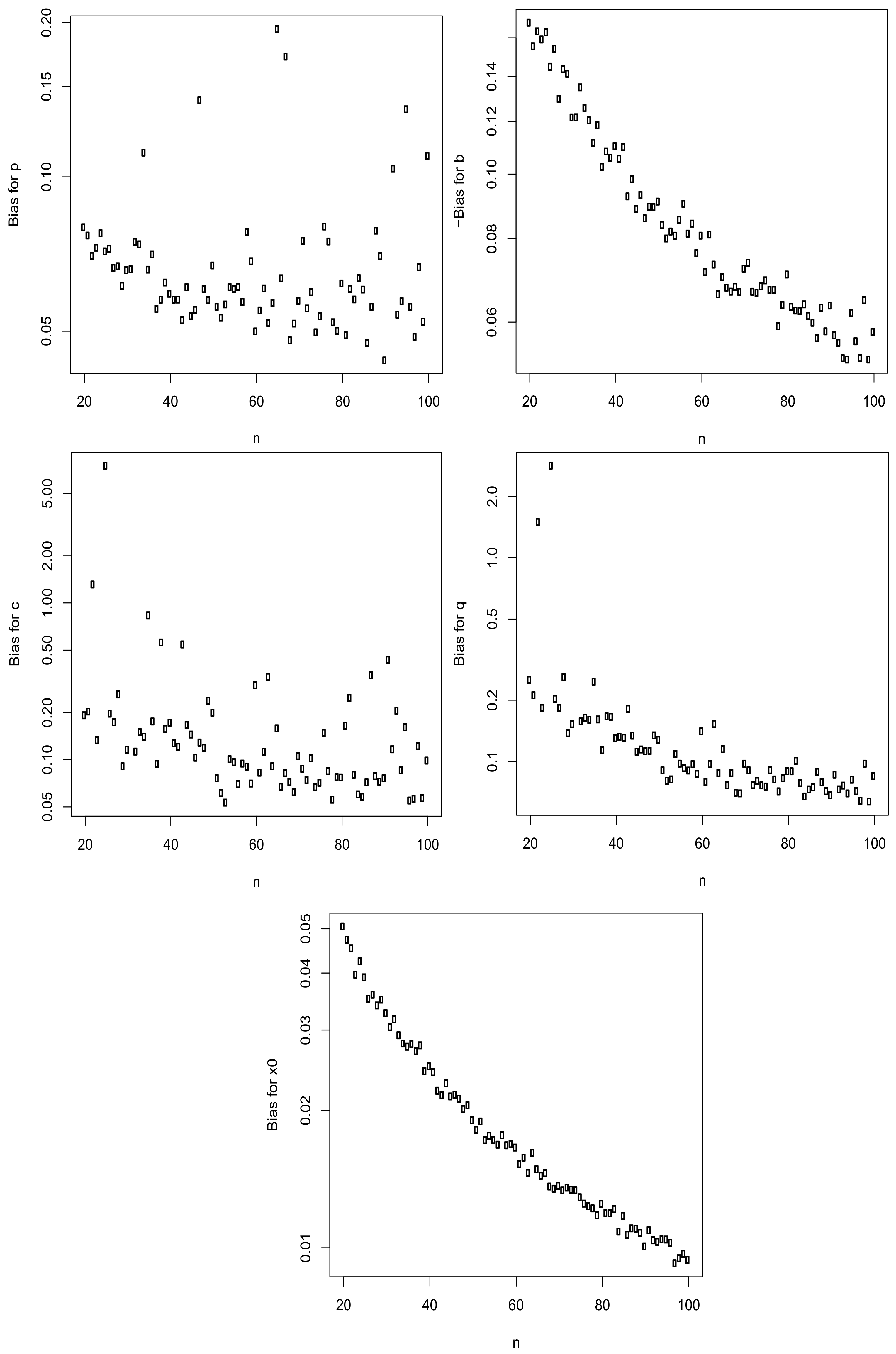
5. Estimation

Suppose $x_1,\dots ,x_n$ is a random sample from (1). In this section, the maximum likelihood estimation of $\left(p,b,c,q,x_0\right)$ is considered and the associated observed information matrix is derived. The log-likelihood function is

$$\begin{array}{ccc}& & {\displaystyle logL\left(p,b,c,q,x_0\right)=nlog\mid b\mid +nlogq-nblogc+(b-1)\sum _{i=1}^{n}log\left(x_i-x_0\right)}\hfill \\ & & {\displaystyle -(q+1)\sum _{i=1}^{n}log{G}_p\left(x_i\right)+p\sum _{i=1}^{n}log\left\{1-\frac{{\left[G_p\left(x_i\right)\right]}^{-q}}{p+1}\right\}.}\hfill \end{array}$$

(24)

The partial derivatives of (24) with respect to the parameters are

$$\begin{array}{ccc}& & {\displaystyle \frac{\partial logL}{\partial p}=-(q+1)\sum _{i=1}^n\frac{1}{G_p\left(x_i\right)}\frac{\partial G_p\left(x_i\right)}{\partial p}+\sum _{i=1}^{n}log\left\{1-\frac{{\left[G_p\left(x_i\right)\right]}^{-q}}{p+1}\right\}}\hfill \\ & & {\displaystyle +p\sum _{i=1}^n{\left\{1-\frac{{\left[G_p\left(x_i\right)\right]}^{-q}}{p+1}\right\}}^{-1}\frac{{\left[G_p\left(x_i\right)\right]}^{-q}}{p+1}\left[\frac{1}{p+1}+\frac{q}{G_p\left(x_i\right)}\frac{\partial G_p\left(x_i\right)}{\partial p}\right],}\hfill \end{array}$$

$$\begin{array}{ccc}& & {\displaystyle \frac{\partial logL}{\partial b}=\frac{n\mathrm{sign}\left(b\right)}{\mid b\mid }-nlogc+\sum _{i=1}^{n}log\left(x_i-x_0\right)-(q+1)\sum _{i=1}^n\frac{1}{G_p\left(x_i\right)}\frac{\partial G_p\left(x_i\right)}{\partial b}}\hfill \\ & & {\displaystyle +\frac{pq}{p+1}\sum _{i=1}^n{\left\{1-\frac{{\left[G_p\left(x_i\right)\right]}^{-q}}{p+1}\right\}}^{-1}{\left[G_p\left(x_i\right)\right]}^{-q-1}\frac{\partial G_p\left(x_i\right)}{\partial b},}\hfill \end{array}$$

$$\begin{array}{ccc}& & {\displaystyle \frac{\partial logL}{\partial c}=-\frac{nb}{c}-(q+1)\sum _{i=1}^n\frac{1}{G_p\left(x_i\right)}\frac{\partial G_p\left(x_i\right)}{\partial c}}\hfill \\ & & {\displaystyle +\frac{pq}{p+1}\sum _{i=1}^n{\left\{1-\frac{{\left[G_p\left(x_i\right)\right]}^{-q}}{p+1}\right\}}^{-1}{\left[G_p\left(x_i\right)\right]}^{-q-1}\frac{\partial G_p\left(x_i\right)}{\partial c},}\hfill \end{array}$$

$$\begin{array}{ccc}& & {\displaystyle \frac{\partial logL}{\partial q}=\frac{n}{q}-\sum _{i=1}^{n}log{G}_p\left(x_i\right)-(q+1)\sum _{i=1}^n\frac{1}{G_p\left(x_i\right)}\frac{\partial G_p\left(x_i\right)}{\partial q}}\hfill \\ & & {\displaystyle +\frac{p}{p+1}\sum _{i=1}^n{\left\{1-\frac{{\left[G_p\left(x_i\right)\right]}^{-q}}{p+1}\right\}}^{-1}{\left[G_p\left(x_i\right)\right]}^{-q}\left[log{G}_p\left(x_i\right)+\frac{q}{G_p\left(x_i\right)}\frac{\partial G_p\left(x_i\right)}{\partial q}\right]}\hfill \end{array}$$

and

$$\begin{array}{ccc}& & {\displaystyle \frac{\partial logL}{\partial x_0}=(1-b)\sum _{i=1}^n\frac{1}{x_i-x_0}-(q+1)\sum _{i=1}^n\frac{1}{G_p\left(x_i\right)}\frac{\partial G_p\left(x_i\right)}{\partial x_0}}\hfill \\ & & {\displaystyle +\frac{pq}{p+1}\sum _{i=1}^n{\left\{1-\frac{{\left[G_p\left(x_i\right)\right]}^{-q}}{p+1}\right\}}^{-1}{\left[G_p\left(x_i\right)\right]}^{-q-1}\frac{\partial G_p\left(x_i\right)}{\partial x_0},}\hfill \end{array}$$

where $\frac{\partial G_p\left(x\right)}{\partial p}=-\frac{1}{q}{(p+1)}^{-\frac{1}{q}-1}$, $\frac{\partial G_p\left(x\right)}{\partial b}={\left(\frac{x-x_0}{c}\right)}^{b}log\left(\frac{x-x_0}{c}\right)$, $\frac{\partial G_p\left(x\right)}{\partial c}=-\frac{b}{c}{\left(\frac{x-x_0}{c}\right)}^b$, $\frac{\partial G_p\left(x\right)}{\partial q}=\frac{1}{q^2}{(p+1)}^{-\frac{1}{q}}log(p+1)$ and $\frac{\partial G_p\left(x\right)}{\partial x_0}=-\frac{b}{c}{\left(\frac{x-x_0}{c}\right)}^{b-1}$. The maximum likelihood estimators of $\left(p,b,c,q,x_0\right)$, say $\left(\widehat{p},\widehat{b},\widehat{c},\widehat{q},\widehat{x_0}\right)$, can be obtained as the simultaneous solutions of $\frac{\partial logL}{\partial p}=0$, $\frac{\partial logL}{\partial b}=0$, $\frac{\partial logL}{\partial c}=0$, $\frac{\partial logL}{\partial q}=0$ and $\frac{\partial logL}{\partial x_0}=0$. The maximum likelihood estimators of $\left(p,b,c,q,x_0\right)$ can also be obtained by directly maximizing (24). In Section 6, the maximum likelihood estimates were obtained by directly maximizing (24). The optim function in R software [6] was used for numerical maximization. optim was executed for a wide range of initial values. optim did not converge for all of the initial values. Whenever optim converged, the maximum likelihood estimates were unique.

Confidence intervals and tests of the hypothesis about $\left(p,b,c,q,x_0\right)$ can be based on the fact that $\left(\widehat{p},\widehat{b},\widehat{c},\widehat{q},\widehat{x_0}\right)$ has an asymptotic normal distribution with the mean $\left(p,b,c,q,x_0\right)$ and covariance matrix ${\mathbf{I}}^{-1}\left(p,b,c,q,x_0\right)$, where $I\left(p,b,c,q,x_0\right)$ denotes the expected information matrix. For a large n, $\mathbf{I}\left(p,b,c,q,x_0\right)$ can be approximated by the observed information matrix $\mathbf{J}\left(p,b,c,q,x_0\right)$. Standard calculations show that

$$\begin{array}{c}\hfill {\displaystyle \mathbf{J}=\left(\begin{array}{ccccc}{J}_{1,1}& J_{1,2}& J_{1,3}& J_{1,4}& J_{1,5}\\ J_{1,2}& J_{2,2}& J_{2,3}& J_{2,4}& J_{2,5}\\ J_{1,3}& J_{2,3}& J_{3,3}& J_{3,4}& J_{3,5}\\ J_{1,4}& J_{2,4}& J_{3,4}& J_{4,4}& J_{4,5}\\ J_{1,5}& J_{2,5}& J_{3,5}& J_{4,5}& J_{5,5}\end{array}\right),}\end{array}$$

(25)

where

$$\begin{array}{ccc}& & {\displaystyle J_{1,1}=-(q+1)\sum _{i=1}^n\left\{\frac{1}{G_p\left(x_i\right)}\frac{{\partial }^2{G}_p\left(x_i\right)}{\partial p^2}-{\left[\frac{1}{G_p\left(x_i\right)}\frac{\partial G_p\left(x_i\right)}{\partial p}\right]}^2\right\}}\hfill \\ & & {\displaystyle +\frac{2}{p+1}\sum _{i=1}^n{\left\{1-\frac{{\left[G_p\left(x_i\right)\right]}^{-q}}{p+1}\right\}}^{-1}{\left[G_p\left(x_i\right)\right]}^{-q}\left[\frac{1}{p+1}+\frac{q}{G_p\left(x_i\right)}\frac{\partial G_p\left(x_i\right)}{\partial p}\right]}\hfill \\ & & {\displaystyle -\frac{p}{{(p+1)}^2}\sum _{i=1}^n{\left\{1-\frac{{\left[G_p\left(x_i\right)\right]}^{-q}}{p+1}\right\}}^{-2}{\left[G_p\left(x_i\right)\right]}^{-2q}{\left[\frac{1}{p+1}+\frac{q}{G_p\left(x_i\right)}\frac{\partial G_p\left(x_i\right)}{\partial p}\right]}^2}\hfill \\ & & {\displaystyle +\frac{p}{p+1}\sum _{i=1}^n{\left\{1-\frac{{\left[G_p\left(x_i\right)\right]}^{-q}}{p+1}\right\}}^{-2}{\left[G_p\left(x_i\right)\right]}^{-q}\{-\frac{2}{{(p+1)}^2}-\frac{2q}{(p+1)G_p\left(x_i\right)}\frac{\partial G_p\left(x_i\right)}{\partial p}}\hfill \\ & & {\displaystyle +\frac{q}{G_p\left(x_i\right)}\frac{{\partial }^2{G}_p\left(x_i\right)}{\partial p^2}-\frac{q(q+1)}{{\left[G_p\left(x_i\right)\right]}^2}{\left[\frac{\partial G_p\left(x_i\right)}{\partial p}\right]}^2\},}\hfill \end{array}$$

$$\begin{array}{ccc}& & {\displaystyle J_{1,2}=(q+1)\sum _{i=1}^n\frac{1}{{\left[G_p\left(x_i\right)\right]}^2}\frac{\partial G_p\left(x_i\right)}{\partial p}\frac{\partial G_p\left(x_i\right)}{\partial b}}\hfill \\ & & {\displaystyle +\frac{q}{p+1}\sum _{i=1}^n{\left\{1-\frac{{\left[G_p\left(x_i\right)\right]}^{-q}}{p+1}\right\}}^{-1}{\left[G_p\left(x_i\right)\right]}^{-q-1}\frac{\partial G_p\left(x_i\right)}{\partial b}}\hfill \\ & & {\displaystyle -\frac{pq}{{(p+1)}^2}\sum _{i=1}^n{\left\{1-\frac{{\left[G_p\left(x_i\right)\right]}^{-q}}{p+1}\right\}}^{-2}{\left[G_p\left(x_i\right)\right]}^{-2q-1}\frac{\partial G_p\left(x_i\right)}{\partial b}\left[\frac{1}{p+1}+\frac{q}{G_p\left(x_i\right)}\frac{\partial G_p\left(x_i\right)}{\partial p}\right]}\hfill \\ & & {\displaystyle +\frac{pq}{p+1}\sum _{i=1}^n{\left\{1-\frac{{\left[G_p\left(x_i\right)\right]}^{-q}}{p+1}\right\}}^{-1}{\left[G_p\left(x_i\right)\right]}^{-q-1}[-\frac{1}{p+1}\frac{\partial G_p\left(x_i\right)}{\partial b}}\hfill \\ & & {\displaystyle -\frac{q+1}{{\left[G_p\left(x_i\right)\right]}^2}\frac{\partial G_p\left(x_i\right)}{\partial p}\frac{\partial G_p\left(x_i\right)}{\partial b}],}\hfill \end{array}$$

$$\begin{array}{ccc}& & {\displaystyle J_{1,3}=(q+1)\sum _{i=1}^n\frac{1}{{\left[G_p\left(x_i\right)\right]}^2}\frac{\partial G_p\left(x_i\right)}{\partial p}\frac{\partial G_p\left(x_i\right)}{\partial c}}\hfill \\ & & {\displaystyle +\frac{q}{p+1}\sum _{i=1}^n{\left\{1-\frac{{\left[G_p\left(x_i\right)\right]}^{-q}}{p+1}\right\}}^{-1}{\left[G_p\left(x_i\right)\right]}^{-q-1}\frac{\partial G_p\left(x_i\right)}{\partial c}}\hfill \\ & & {\displaystyle -\frac{pq}{{(p+1)}^2}\sum _{i=1}^n{\left\{1-\frac{{\left[G_p\left(x_i\right)\right]}^{-q}}{p+1}\right\}}^{-2}{\left[G_p\left(x_i\right)\right]}^{-2q-1}\frac{\partial G_p\left(x_i\right)}{\partial c}\left[\frac{1}{p+1}+\frac{q}{G_p\left(x_i\right)}\frac{\partial G_p\left(x_i\right)}{\partial p}\right]}\hfill \\ & & {\displaystyle +\frac{pq}{p+1}\sum _{i=1}^n{\left\{1-\frac{{\left[G_p\left(x_i\right)\right]}^{-q}}{p+1}\right\}}^{-1}{\left[G_p\left(x_i\right)\right]}^{-q-1}[-\frac{1}{p+1}\frac{\partial G_p\left(x_i\right)}{\partial c}}\hfill \\ & & {\displaystyle -\frac{q+1}{{\left[G_p\left(x_i\right)\right]}^2}\frac{\partial G_p\left(x_i\right)}{\partial p}\frac{\partial G_p\left(x_i\right)}{\partial c}],}\hfill \end{array}$$

$$\begin{array}{ccc}& & {\displaystyle J_{1,4}=-\sum _{i=1}^n\frac{1}{G_p\left(x_i\right)}\frac{\partial G_p\left(x_i\right)}{\partial p}}\hfill \\ & & {\displaystyle +(q+1)\sum _{i=1}^n\frac{1}{{\left[G_p\left(x_i\right)\right]}^2}\frac{\partial G_p\left(x_i\right)}{\partial p}\frac{\partial G_p\left(x_i\right)}{\partial q}-(q+1)\sum _{i=1}^n\frac{1}{G_p\left(x_i\right)}\frac{{\partial }^2{G}_p\left(x_i\right)}{\partial p\partial q}}\hfill \\ & & {\displaystyle +\frac{1}{p+1}\sum _{i=1}^n{\left\{1-\frac{{\left[G_p\left(x_i\right)\right]}^{-q}}{p+1}\right\}}^{-1}{\left[G_p\left(x_i\right)\right]}^{-q}\left[log{G}_p\left(x_i\right)+\frac{q}{G_p\left(x_i\right)}\frac{\partial G_p\left(x_i\right)}{\partial q}\right]}\hfill \\ & & {\displaystyle -\frac{p}{{(p+1)}^2}\sum _{i=1}^n{\left\{1-\frac{{\left[G_p\left(x_i\right)\right]}^{-q}}{p+1}\right\}}^{-2}{\left[G_p\left(x_i\right)\right]}^{-3q}\left[\frac{1}{p+1}+\frac{q}{G_p\left(x_i\right)}\frac{\partial G_p\left(x_i\right)}{\partial p}\right][log{G}_p\left(x_i\right)}\hfill \\ & & {\displaystyle +\frac{q}{G_p\left(x_i\right)}\frac{\partial G_p\left(x_i\right)}{\partial q}]}\hfill \\ & & {\displaystyle +\frac{p}{p+1}\sum _{i=1}^n{\left\{1-\frac{{\left[G_p\left(x_i\right)\right]}^{-q}}{p+1}\right\}}^{-1}{\left[G_p\left(x_i\right)\right]}^{-q}[-\frac{1}{p+1}log{G}_p\left(x_i\right)-\frac{q}{(p+1)G_p\left(x_i\right)}\frac{\partial G_p\left(x_i\right)}{\partial q}}\hfill \\ & & {\displaystyle +\frac{1}{G_p\left(x_i\right)}\frac{\partial G_p\left(x_i\right)}{\partial p}+\frac{q}{G_p\left(x_i\right)}\frac{{\partial }^2{G}_p\left(x_i\right)}{\partial p\partial q}}\hfill \\ & & {\displaystyle -\frac{q}{G_p\left(x_i\right)}log{G}_p\left(x_i\right)\frac{\partial G_p\left(x_i\right)}{\partial p}-\frac{q(q+1)}{{\left[G_p\left(x_i\right)\right]}^2}\frac{\partial G_p\left(x_i\right)}{\partial p}\frac{\partial G_p\left(x_i\right)}{\partial q}],}\hfill \end{array}$$

$$\begin{array}{ccc}& & {\displaystyle J_{1,5}=(q+1)\sum _{i=1}^n\frac{1}{{\left[G_p\left(x_i\right)\right]}^2}\frac{\partial G_p\left(x_i\right)}{\partial p}\frac{\partial G_p\left(x_i\right)}{\partial x_0}}\hfill \\ & & {\displaystyle +\frac{q}{p+1}\sum _{i=1}^n{\left\{1-\frac{{\left[G_p\left(x_i\right)\right]}^{-q}}{p+1}\right\}}^{-1}{\left[G_p\left(x_i\right)\right]}^{-q-1}\frac{\partial G_p\left(x_i\right)}{\partial x_0}}\hfill \\ & & {\displaystyle -\frac{pq}{{(p+1)}^2}\sum _{i=1}^n{\left\{1-\frac{{\left[G_p\left(x_i\right)\right]}^{-q}}{p+1}\right\}}^{-2}{\left[G_p\left(x_i\right)\right]}^{-2q-1}\frac{\partial G_p\left(x_i\right)}{\partial x_0}\left[\frac{1}{p+1}+\frac{q}{G_p\left(x_i\right)}\frac{\partial G_p\left(x_i\right)}{\partial p}\right]}\hfill \\ & & {\displaystyle +\frac{pq}{p+1}\sum _{i=1}^n{\left\{1-\frac{{\left[G_p\left(x_i\right)\right]}^{-q}}{p+1}\right\}}^{-1}{\left[G_p\left(x_i\right)\right]}^{-q-1}[-\frac{1}{p+1}\frac{\partial G_p\left(x_i\right)}{\partial x_0}}\hfill \\ & & {\displaystyle -\frac{q+1}{{\left[G_p\left(x_i\right)\right]}^2}\frac{\partial G_p\left(x_i\right)}{\partial p}\frac{\partial G_p\left(x_i\right)}{\partial x_0}],}\hfill \end{array}$$

$$\begin{array}{ccc}& & {\displaystyle J_{2,2}=\frac{2n\delta \left(b\right)}{\mid b\mid }-\frac{n{\left[\mathrm{sign}\left(b\right)\right]}^2}{b^2}}\hfill \\ & & {\displaystyle +(q+1)\sum _{i=1}^n{\left[\frac{1}{G_p\left(x_i\right)}\frac{\partial G_p\left(x_i\right)}{\partial b}\right]}^2-(q+1)\sum _{i=1}^n\frac{1}{G_p\left(x_i\right)}\frac{{\partial }^2{G}_p\left(x_i\right)}{\partial b^2}}\hfill \\ & & {\displaystyle -\frac{p{q}^2}{{(p+1)}^2}\sum _{i=1}^n{\left\{1-\frac{{\left[G_p\left(x_i\right)\right]}^{-q}}{p+1}\right\}}^{-2}{\left\{{\left[G_p\left(x_i\right)\right]}^{-q-1}\frac{\partial G_p\left(x_i\right)}{\partial b}\right\}}^2}\hfill \\ & & {\displaystyle +\frac{pq}{p+1}\sum _{i=1}^n{\left\{1-\frac{{\left[G_p\left(x_i\right)\right]}^{-q}}{p+1}\right\}}^{-1}{\left[G_p\left(x_i\right)\right]}^{-q-1}\left\{\frac{{\partial }^2{G}_p\left(x_i\right)}{\partial b^2}-\frac{q+1}{G_p\left(x_i\right)}{\left[\frac{\partial G_p\left(x_i\right)}{\partial b}\right]}^2\right\},}\hfill \end{array}$$

$$\begin{array}{ccc}& & {\displaystyle J_{2,3}=-\frac{n}{c}+(q+1)\sum _{i=1}^n\frac{1}{{\left[G_p\left(x_i\right)\right]}^2}\frac{\partial G_p\left(x_i\right)}{\partial b}\frac{\partial G_p\left(x_i\right)}{\partial c}-(q+1)\sum _{i=1}^n\frac{1}{G_p\left(x_i\right)}\frac{{\partial }^2{G}_p\left(x_i\right)}{\partial b\partial c}}\hfill \\ & & {\displaystyle -\frac{p{q}^2}{{(p+1)}^2}\sum _{i=1}^n{\left\{1-\frac{{\left[G_p\left(x_i\right)\right]}^{-q}}{p+1}\right\}}^{-2}{\left[G_p\left(x_i\right)\right]}^{-2q-2}\frac{\partial G_p\left(x_i\right)}{\partial b}\frac{\partial G_p\left(x_i\right)}{\partial c}}\hfill \\ & & {\displaystyle +\frac{pq}{p+1}\sum _{i=1}^n{\left\{1-\frac{{\left[G_p\left(x_i\right)\right]}^{-q}}{p+1}\right\}}^{-1}{\left[G_p\left(x_i\right)\right]}^{-q-1}\left\{\frac{{\partial }^2{G}_p\left(x_i\right)}{\partial b\partial c}-\frac{q+1}{G_p\left(x_i\right)}\frac{\partial G_p\left(x_i\right)}{\partial b}\frac{\partial G_p\left(x_i\right)}{\partial c}\right\},}\hfill \end{array}$$

$$\begin{array}{ccc}& & {\displaystyle J_{2,4}=-\sum _{i=1}^n\frac{1}{G_p\left(x_i\right)}\frac{\partial G_p\left(x_i\right)}{\partial b}+(q+1)\sum _{i=1}^n\frac{1}{{\left[G_p\left(x_i\right)\right]}^2}\frac{\partial G_p\left(x_i\right)}{\partial b}\frac{\partial G_p\left(x_i\right)}{\partial q}}\hfill \\ & & {\displaystyle +\frac{p}{p+1}\sum _{i=1}^n{\left\{1-\frac{{\left[G_p\left(x_i\right)\right]}^{-q}}{p+1}\right\}}^{-1}{\left[G_p\left(x_i\right)\right]}^{-q-1}\frac{\partial G_p\left(x_i\right)}{\partial b}}\hfill \\ & & {\displaystyle -\frac{p{q}^2}{{(p+1)}^2}\sum _{i=1}^n{\left\{1-\frac{{\left[G_p\left(x_i\right)\right]}^{-q}}{p+1}\right\}}^{-2}{\left[G_p\left(x_i\right)\right]}^{-2q-2}\frac{\partial G_p\left(x_i\right)}{\partial b}\frac{\partial G_p\left(x_i\right)}{\partial q}}\hfill \\ & & {\displaystyle -\frac{pq(q+1)}{p+1}\sum _{i=1}^n{\left\{1-\frac{{\left[G_p\left(x_i\right)\right]}^{-q}}{p+1}\right\}}^{-1}{\left[G_p\left(x_i\right)\right]}^{-q-2}\frac{\partial G_p\left(x_i\right)}{\partial b}\frac{\partial G_p\left(x_i\right)}{\partial q}}\hfill \\ & & {\displaystyle +\frac{pq}{p+1}\sum _{i=1}^n{\left\{1-\frac{{\left[G_p\left(x_i\right)\right]}^{-q}}{p+1}\right\}}^{-1}{\left[G_p\left(x_i\right)\right]}^{-q-1}\frac{{\partial }^2{G}_p\left(x_i\right)}{\partial b\partial q},}\hfill \end{array}$$

$$\begin{array}{ccc}& & {\displaystyle J_{2,5}=\sum _{i=1}^n\frac{1}{x_0-x_i}+(q+1)\sum _{i=1}^n\frac{1}{{\left[G_p\left(x_i\right)\right]}^2}\frac{\partial G_p\left(x_i\right)}{\partial b}\frac{\partial G_p\left(x_i\right)}{\partial x_0}-(q+1)\sum _{i=1}^n\frac{1}{G_p\left(x_i\right)}\frac{{\partial }^2{G}_p\left(x_i\right)}{\partial b\partial x_0}}\hfill \\ & & {\displaystyle -\frac{p{q}^2}{{(p+1)}^2}\sum _{i=1}^n{\left\{1-\frac{{\left[G_p\left(x_i\right)\right]}^{-q}}{p+1}\right\}}^{-2}{\left[G_p\left(x_i\right)\right]}^{-2q-2}\frac{\partial G_p\left(x_i\right)}{\partial b}\frac{\partial G_p\left(x_i\right)}{\partial x_0}}\hfill \\ & & {\displaystyle +\frac{pq}{p+1}\sum _{i=1}^n{\left\{1-\frac{{\left[G_p\left(x_i\right)\right]}^{-q}}{p+1}\right\}}^{-1}{\left[G_p\left(x_i\right)\right]}^{-q-1}\left\{\frac{{\partial }^2{G}_p\left(x_i\right)}{\partial b\partial x_0}-\frac{q+1}{G_p\left(x_i\right)}\frac{\partial G_p\left(x_i\right)}{\partial b}\frac{\partial G_p\left(x_i\right)}{\partial x_0}\right\},}\hfill \end{array}$$

$$\begin{array}{ccc}& & {\displaystyle J_{3,3}=\frac{nb}{c^2}+(q+1)\sum _{i=1}^n{\left[\frac{1}{G_p\left(x_i\right)}\frac{\partial G_p\left(x_i\right)}{\partial c}\right]}^2-(q+1)\sum _{i=1}^n\frac{1}{G_p\left(x_i\right)}\frac{{\partial }^2{G}_p\left(x_i\right)}{\partial c^2}}\hfill \\ & & {\displaystyle -\frac{p{q}^2}{{(p+1)}^2}\sum _{i=1}^n{\left\{1-\frac{{\left[G_p\left(x_i\right)\right]}^{-q}}{p+1}\right\}}^{-2}{\left[G_p\left(x_i\right)\right]}^{-2q-2}{\left[\frac{\partial G_p\left(x_i\right)}{\partial c}\right]}^2}\hfill \\ & & {\displaystyle -\frac{pq(q+1)}{p+1}\sum _{i=1}^n{\left\{1-\frac{{\left[G_p\left(x_i\right)\right]}^{-q}}{p+1}\right\}}^{-1}{\left[G_p\left(x_i\right)\right]}^{-q-2}\frac{\partial G_p\left(x_i\right)}{\partial c}}\hfill \\ & & {\displaystyle +\frac{pq}{p+1}\sum _{i=1}^n{\left\{1-\frac{{\left[G_p\left(x_i\right)\right]}^{-q}}{p+1}\right\}}^{-1}{\left[G_p\left(x_i\right)\right]}^{-q-1}\frac{{\partial }^2{G}_p\left(x_i\right)}{\partial c^2},}\hfill \end{array}$$

$$\begin{array}{ccc}& & {\displaystyle J_{3,4}=-\sum _{i=1}^n\frac{1}{G_p\left(x_i\right)}\frac{\partial G_p\left(x_i\right)}{\partial c}+(q+1)\sum _{i=1}^n\frac{1}{{\left[G_p\left(x_i\right)\right]}^2}\frac{\partial G_p\left(x_i\right)}{\partial c}\frac{\partial G_p\left(x_i\right)}{\partial q}}\hfill \\ & & {\displaystyle +\frac{p}{p+1}\sum _{i=1}^n{\left\{1-\frac{{\left[G_p\left(x_i\right)\right]}^{-q}}{p+1}\right\}}^{-1}{\left[G_p\left(x_i\right)\right]}^{-q-1}\frac{\partial G_p\left(x_i\right)}{\partial c}}\hfill \\ & & {\displaystyle -\frac{pq}{{(p+1)}^2}\sum _{i=1}^n{\left\{1-\frac{{\left[G_p\left(x_i\right)\right]}^{-q}}{p+1}\right\}}^{-2}{\left[G_p\left(x_i\right)\right]}^{-2q-1}\frac{\partial G_p\left(x_i\right)}{\partial c}\left[log{G}_p\left(x_i\right)+\frac{q}{G_p\left(x_i\right)}\frac{\partial G_p\left(x_i\right)}{\partial q}\right]}\hfill \\ & & {\displaystyle -\frac{pq}{p+1}\sum _{i=1}^n{\left\{1-\frac{{\left[G_p\left(x_i\right)\right]}^{-q}}{p+1}\right\}}^{-1}{\left[G_p\left(x_i\right)\right]}^{-q-1}\frac{\partial G_p\left(x_i\right)}{\partial c}\left[log{G}_p\left(x_i\right)+\frac{q+1}{G_p\left(x_i\right)}\frac{\partial G_p\left(x_i\right)}{\partial q}\right],}\hfill \end{array}$$

$$\begin{array}{ccc}& & {\displaystyle J_{3,5}=(q+1)\sum _{i=1}^n\frac{1}{{\left[G_p\left(x_i\right)\right]}^2}\frac{\partial G_p\left(x_i\right)}{\partial c}\frac{\partial G_p\left(x_i\right)}{\partial x_0}-(q+1)\sum _{i=1}^n\frac{1}{G_p\left(x_i\right)}\frac{{\partial }^2{G}_p\left(x_i\right)}{\partial c\partial x_0}}\hfill \\ & & {\displaystyle +\frac{p{q}^2}{{(p+1)}^2}\sum _{i=1}^n{\left\{1-\frac{{\left[G_p\left(x_i\right)\right]}^{-q}}{p+1}\right\}}^{-2}{\left[G_p\left(x_i\right)\right]}^{-2q-2}\frac{\partial G_p\left(x_i\right)}{\partial c}\frac{\partial G_p\left(x_i\right)}{\partial x_0}}\hfill \\ & & {\displaystyle -\frac{pq(q+1)}{p+1}\sum _{i=1}^n{\left\{1-\frac{{\left[G_p\left(x_i\right)\right]}^{-q}}{p+1}\right\}}^{-1}{\left[G_p\left(x_i\right)\right]}^{-q-2}\frac{\partial G_p\left(x_i\right)}{\partial c}\frac{\partial G_p\left(x_i\right)}{\partial x_0}}\hfill \\ & & {\displaystyle +\frac{pq}{p+1}\sum _{i=1}^n{\left\{1-\frac{{\left[G_p\left(x_i\right)\right]}^{-q}}{p+1}\right\}}^{-1}{\left[G_p\left(x_i\right)\right]}^{-q-1}\frac{{\partial }^2{G}_p\left(x_i\right)}{\partial c\partial x_0},}\hfill \end{array}$$

$$\begin{array}{ccc}& & {\displaystyle J_{4,4}=-\frac{n}{q^2}-2\sum _{i=1}^n\frac{1}{G_p\left(x_i\right)}\frac{\partial G_p\left(x_i\right)}{\partial q}}\hfill \\ & & {\displaystyle +(q+1)\sum _{i=1}^n{\left[\frac{1}{G_p\left(x_i\right)}\frac{\partial G_p\left(x_i\right)}{\partial q}\right]}^2-(q+1)\sum _{i=1}^n\frac{1}{G_p\left(x_i\right)}\frac{{\partial }^2{G}_p\left(x_i\right)}{\partial q^2}}\hfill \\ & & {\displaystyle -\frac{p}{{(p+1)}^2}\sum _{i=1}^n{\left\{1-\frac{{\left[G_p\left(x_i\right)\right]}^{-q}}{p+1}\right\}}^{-2}{\left[G_p\left(x_i\right)\right]}^{-2q}{\left[log{G}_p\left(x_i\right)+\frac{q}{G_p\left(x_i\right)}\frac{\partial G_p\left(x_i\right)}{\partial q}\right]}^2}\hfill \\ & & {\displaystyle -\frac{p}{p+1}\sum _{i=1}^n{\left\{1-\frac{{\left[G_p\left(x_i\right)\right]}^{-q}}{p+1}\right\}}^{-1}{\left[G_p\left(x_i\right)\right]}^{-q}{\left[log{G}_p\left(x_i\right)+\frac{q}{G_p\left(x_i\right)}\frac{\partial G_p\left(x_i\right)}{\partial q}\right]}^2}\hfill \\ & & {\displaystyle +\frac{p}{p+1}\sum _{i=1}^n{\left\{1-\frac{{\left[G_p\left(x_i\right)\right]}^{-q}}{p+1}\right\}}^{-1}{\left[G_p\left(x_i\right)\right]}^{-q}\{\frac{2}{G_p\left(x_i\right)}\frac{\partial G_p\left(x_i\right)}{\partial q}}\hfill \\ & & {\displaystyle -\frac{q}{{\left[G_p\left(x_i\right)\right]}^2}{\left[\frac{\partial G_p\left(x_i\right)}{\partial q}\right]}^2+\frac{q}{G_p\left(x_i\right)}\frac{{\partial }^2{G}_p\left(x_i\right)}{\partial q^2}\},}\hfill \end{array}$$

$$\begin{array}{ccc}& & {\displaystyle J_{4,5}=-\sum _{i=1}^n\frac{1}{G_p\left(x_i\right)}\frac{\partial G_p\left(x_i\right)}{\partial x_0}}\hfill \\ & & {\displaystyle +(q+1)\sum _{i=1}^n\frac{1}{{\left[G_p\left(x_i\right)\right]}^2}\frac{\partial G_p\left(x_i\right)}{\partial q}\frac{\partial G_p\left(x_i\right)}{\partial x_0}}\hfill \\ & & {\displaystyle +\frac{pq}{{(p+1)}^2}\sum _{i=1}^n{\left\{1-\frac{{\left[G_p\left(x_i\right)\right]}^{-q}}{p+1}\right\}}^{-2}{\left[G_p\left(x_i\right)\right]}^{-2q-1}\frac{\partial G_p\left(x_i\right)}{\partial x_0}\left[log{G}_p\left(x_i\right)+\frac{q}{G_p\left(x_i\right)}\frac{\partial G_p\left(x_i\right)}{\partial q}\right]}\hfill \\ & & {\displaystyle -\frac{pq}{p+1}\sum _{i=1}^n{\left\{1-\frac{{\left[G_p\left(x_i\right)\right]}^{-q}}{p+1}\right\}}^{-1}{\left[G_p\left(x_i\right)\right]}^{-q-1}\frac{\partial G_p\left(x_i\right)}{\partial x_0}\left[log{G}_p\left(x_i\right)+\frac{q}{G_p\left(x_i\right)}\frac{\partial G_p\left(x_i\right)}{\partial q}\right]}\hfill \\ & & {\displaystyle +\frac{p}{p+1}\sum _{i=1}^n{\left\{1-\frac{{\left[G_p\left(x_i\right)\right]}^{-q}}{p+1}\right\}}^{-1}{\left[G_p\left(x_i\right)\right]}^{-q}\left\{\frac{1}{G_p\left(x_i\right)}\frac{\partial G_p\left(x_i\right)}{\partial x_0}-\frac{q}{{\left[G_p\left(x_i\right)\right]}^2}\frac{\partial G_p\left(x_i\right)}{\partial q}\frac{\partial G_p\left(x_i\right)}{\partial x_0}\right\}}\hfill \end{array}$$

and

$$\begin{array}{ccc}& & {\displaystyle J_{5,5}=(1-b)\sum _{i=1}^n\frac{1}{{\left(x_i-x_0\right)}^2}+(q+1)\sum _{i=1}^n{\left[\frac{1}{G_p\left(x_i\right)}\frac{\partial G_p\left(x_i\right)}{\partial x_0}\right]}^2-(q+1)\sum _{i=1}^n\frac{1}{G_p\left(x_i\right)}\frac{{\partial }^2{G}_p\left(x_i\right)}{\partial x_0^2}}\hfill \\ & & {\displaystyle +\frac{p{q}^2}{{(p+1)}^2}\sum _{i=1}^n{\left\{1-\frac{{\left[G_p\left(x_i\right)\right]}^{-q}}{p+1}\right\}}^{-2}{\left[G_p\left(x_i\right)\right]}^{-2q-2}{\left[\frac{\partial G_p\left(x_i\right)}{\partial x_0}\right]}^2}\hfill \\ & & {\displaystyle -\frac{pq(q+1)}{p+1}\sum _{i=1}^n{\left\{1-\frac{{\left[G_p\left(x_i\right)\right]}^{-q}}{p+1}\right\}}^{-1}{\left[G_p\left(x_i\right)\right]}^{-q-2}{\left[\frac{\partial G_p\left(x_i\right)}{\partial x_0}\right]}^2}\hfill \\ & & {\displaystyle +\frac{pq}{p+1}\sum _{i=1}^n{\left\{1-\frac{{\left[G_p\left(x_i\right)\right]}^{-q}}{p+1}\right\}}^{-1}{\left[G_p\left(x_i\right)\right]}^{-q-1}\frac{{\partial }^2{G}_p\left(x_i\right)}{\partial x_0^2},}\hfill \end{array}$$

where $\frac{{\partial }^2{G}_p\left(x\right)}{\partial p^2}=\frac{1}{q}\left(\frac{1}{q}+1\right){(p+1)}^{-\frac{1}{q}-2}$, $\frac{{\partial }^2{G}_p\left(x\right)}{\partial p\partial q}=\frac{1}{q^2}{(p+1)}^{-\frac{1}{q}-1}-\frac{1}{q^3}{(p+1)}^{-\frac{1}{q}-1}log(p+1)$, $\frac{{\partial }^2{G}_p\left(x\right)}{\partial b^2}={\left(\frac{x-x_0}{c}\right)}^b{\left[log\left(\frac{x-x_0}{c}\right)\right]}^2$, $\frac{{\partial }^2{G}_p\left(x\right)}{\partial b\partial c}=-\frac{b}{c}{\left(\frac{x-x_0}{c}\right)}^{b}log\left(\frac{x-x_0}{c}\right)-\frac{1}{c}{\left(\frac{x-x_0}{c}\right)}^b$, $\frac{{\partial }^2{G}_p\left(x\right)}{\partial b\partial x_0}=-\frac{b}{c}$${\left(\frac{x-x_0}{c}\right)}^{b-1}$ log$\left(\frac{x-x_0}{c}\right)$−$\frac{1}{c}$${\left(\frac{x-x_0}{c}\right)}^{b-1}$, $\frac{{\partial }^2{G}_p\left(x\right)}{\partial c^2}=\frac{b(b+1)}{c^2}{\left(\frac{x-x_0}{c}\right)}^b$, $\frac{{\partial }^2{G}_p\left(x\right)}{\partial c\partial x_0}=\frac{b^2}{c^2}{\left(\frac{x-x_0}{c}\right)}^{b-1}$, $\frac{{\partial }^2{G}_p\left(x\right)}{\partial q^2}$=$\frac{1}{q^4}$${(p+1)}^{-\frac{1}{q}}$ ${\left[log(p+1)\right]}^2$−$\frac{2}{q^3}$${(p+1)}^{-\frac{1}{q}}$$log(p+1)$ and $\frac{{\partial }^2{G}_p\left(x\right)}{\partial x_0^2}=\frac{b(b-1)}{c^2}{\left(\frac{x-x_0}{c}\right)}^{b-2}$. In addition, $\delta (·)$ denotes the Dirac delta function.

The $100(1-\alpha )$ percent confidence intervals for p, b, c, q and $x_0$ based on (25) are

$$\begin{array}{c}\hfill {\displaystyle \widehat{p}\pm z_{1-\frac{\alpha }{2}}{\widehat{J}}^{1,1},}\end{array}$$

$$\begin{array}{c}\hfill {\displaystyle \widehat{b}\pm z_{1-\frac{\alpha }{2}}{\widehat{J}}^{2,2},}\end{array}$$

$$\begin{array}{c}\hfill {\displaystyle \widehat{c}\pm z_{1-\frac{\alpha }{2}}{\widehat{J}}^{3,3},}\end{array}$$

$$\begin{array}{c}\hfill {\displaystyle \widehat{q}\pm z_{1-\frac{\alpha }{2}}{\widehat{J}}^{4,4}}\end{array}$$

and

$$\begin{array}{c}\hfill {\displaystyle \widehat{x_0}\pm z_{1-\frac{\alpha }{2}}{\widehat{J}}^{5,5},}\end{array}$$

respectively, where $z_{1-\frac{\alpha }{2}}$ denotes the $100\left(1-\frac{\alpha }{2}\right)$ percentile of the standard normal distribution and ${\widehat{J}}^{j,j}$, $j=1,2,\dots ,5$ denotes the $(j,j)$th element of the inverse of $\mathbf{J}$ with $\left(p,b,c,q,x_0\right)$ when it is replaced by $\left(\widehat{p},\widehat{b},\widehat{c},\widehat{q},\widehat{x_0}\right)$.

6. Simulation Study

In this section, a simulation study is conducted to check the finite sample performance of $\left(\widehat{p},\widehat{b},\widehat{c},\widehat{q},\widehat{x_0}\right)$, which was detailed in Section 5. The finite sample performance is checked with respect to bias and the mean squared error. The following scheme was used:

(a)

Set $p=0$, $b=1$, $c=1$, $q=1$, $x_0=0$ and $n=20$;

(b)

Simulate 10,000 random samples each of size n from (1), the inverse method and the quantile function (detailed in Section 4.2 of [1]);

(c)

Fit (1) to each of the 10,000 samples by the method of maximum likelihood in Section 5, and let $\left({\widehat{p}}^i,{\widehat{b}}^i,{\widehat{c}}^i,{\widehat{q}}^i,{\widehat{x_0}}^i\right)$ denote the maximum likelihood estimates for the ith sample;

(d)

Compute the biases as

$$\begin{array}{c}\hfill {\displaystyle \mathrm{Bias}\left(\widehat{e}\right)=\frac{1}{10000}\sum _{i=1}^{10000}\left({\widehat{e}}^i-e\right)}\end{array}$$

for $e=p,b,c,q,x_0$;

(e)

Compute the mean squared errors as

$$\begin{array}{c}\hfill {\displaystyle \mathrm{MSE}\left(\widehat{e}\right)=\frac{1}{1000}\sum _{i=1}^{1000}{\left({\widehat{e}}^i-e\right)}^2}\end{array}$$

for $e=p,b,c,q,x_0$;

(f)

Repeat steps (b) to (e) for $n=21,22,\dots ,100$.

The biases are plotted in Figure 1. The mean squared errors are plotted in Figure 2. The numerical values of the biases and mean squared errors are given in Table 1 and Table 2.

Figure 1. Biases versus $n=20,21,\dots ,100$. The y axes are in log scale.

Figure 2. Mean squared errors versus $n=20,21,\dots ,100$. The y axes are in log scale.

Table 1. Biases of $\widehat{p}$, $\widehat{b}$, $\widehat{c}$, $\widehat{q}$ and $\widehat{x_0}$.

n	Bias for $\widehat{\mathit{p}}$	Bias for $\widehat{\mathit{b}}$	Bias for $\widehat{\mathit{c}}$	Bias for $\widehat{\mathit{q}}$	Bias for $\widehat{{\mathit{x}}_0}$
20	0.080	−0.169	0.192	0.251	0.051
21	0.077	−0.155	0.203	0.211	0.047
22	0.070	−0.164	1.308	1.494	0.045
23	0.073	−0.159	0.133	0.183	0.040
24	0.078	−0.163	2.497	4.725	0.042
25	0.072	−0.145	7.497	2.826	0.039
26	0.072	−0.154	0.196	0.202	0.035
27	0.066	−0.130	0.173	0.183	0.036
28	0.067	−0.144	0.260	0.259	0.034
29	0.061	−0.141	0.091	0.137	0.035
30	0.066	−0.122	0.115	0.152	0.033
31	0.066	−0.122	4.587	3.811	0.030
32	0.075	−0.135	0.112	0.157	0.032
33	0.074	−0.126	0.150	0.164	0.029
34	0.111	−0.120	0.140	0.160	0.028
35	0.066	−0.111	0.833	0.246	0.028
36	0.071	−0.118	0.175	0.161	0.028
37	0.055	−0.102	0.094	0.114	0.027
38	0.058	−0.108	0.558	0.166	0.028
39	0.062	−0.106	0.157	0.166	0.024
40	0.059	−0.110	0.172	0.130	0.025
41	0.058	−0.105	0.127	0.132	0.024
42	0.058	−0.110	0.120	0.130	0.022
43	0.053	−0.093	0.543	0.181	0.022
44	0.061	−0.098	0.166	0.134	0.023
45	0.053	−0.089	0.144	0.111	0.021
46	0.055	−0.093	0.103	0.114	0.022
47	0.141	−0.086	0.128	0.112	0.021
48	0.060	−0.089	0.119	0.113	0.020
49	0.057	−0.089	0.237	0.134	0.021
50	0.067	−0.091	0.199	0.127	0.019
51	0.056	−0.084	0.076	0.090	0.018
52	0.053	−0.080	0.061	0.080	0.019
53	0.056	−0.082	0.053	0.082	0.017
54	0.061	−0.081	0.101	0.109	0.018
55	0.060	−0.085	0.096	0.097	0.017
56	0.061	−0.090	0.070	0.093	0.017
57	0.057	−0.081	0.094	0.090	0.018
58	0.078	−0.084	0.090	0.097	0.017
59	0.068	−0.076	0.070	0.087	0.017
60	0.050	−0.081	0.299	0.140	0.017
61	0.055	−0.071	0.083	0.079	0.015
62	0.061	−0.081	0.112	0.097	0.016
63	0.052	−0.073	0.337	0.153	0.015
64	0.057	−0.066	0.091	0.088	0.016
65	0.194	−0.070	0.158	0.115	0.015
66	0.063	−0.068	0.067	0.076	0.014
67	0.172	−0.067	0.082	0.088	0.015
68	0.048	−0.068	0.072	0.070	0.014
69	0.052	−0.067	0.062	0.070	0.013
70	0.057	−0.072	0.105	0.097	0.014
71	0.075	−0.074	0.087	0.090	0.013
72	0.055	−0.067	0.074	0.077	0.014
73	0.060	−0.066	0.102	0.080	0.013
74	0.050	−0.068	0.067	0.076	0.013
75	0.053	−0.069	0.071	0.075	0.013
76	0.080	−0.067	0.148	0.091	0.012
77	0.075	−0.067	0.085	0.081	0.012
78	0.052	−0.059	0.055	0.071	0.012
79	0.050	−0.064	0.077	0.083	0.012
80	0.062	−0.071	0.077	0.090	0.012
81	0.049	−0.063	0.165	0.089	0.012
82	0.060	−0.062	0.247	0.101	0.012
83	0.058	−0.062	0.080	0.078	0.012
84	0.063	−0.064	0.060	0.067	0.011
85	0.060	−0.061	0.058	0.073	0.012
86	0.047	−0.060	0.071	0.075	0.011
87	0.056	−0.057	0.345	0.089	0.011
88	0.078	−0.063	0.078	0.079	0.011
89	0.070	−0.058	0.072	0.071	0.011
90	0.044	−0.064	0.076	0.068	0.010
91	0.940	−0.057	0.433	0.086	0.011
92	0.104	−0.056	0.116	0.073	0.010
93	0.054	−0.053	0.205	0.076	0.010
94	0.057	−0.053	0.085	0.070	0.010
95	0.135	−0.062	0.161	0.081	0.010
96	0.056	−0.056	0.055	0.071	0.010
97	0.049	−0.053	0.056	0.064	0.009
98	0.067	−0.065	0.122	0.097	0.009
99	0.052	−0.053	0.057	0.063	0.010
100	0.110	−0.058	0.099	0.085	0.009

Table 2. Mean squared errors of $\widehat{p}$, $\widehat{b}$, $\widehat{c}$, $\widehat{q}$ and $\widehat{x_0}$.

n	MSE for $\widehat{\mathit{p}}$	MSE for $\widehat{\mathit{b}}$	MSE for $\widehat{\mathit{c}}$	MSE for $\widehat{\mathit{q}}$	MSE for $\widehat{{\mathit{x}}_0}$
20	0.029	0.079	1.514	0.758	0.005
21	0.067	0.079	1.934	0.404	0.005
22	0.015	0.073	1223.421	1613.096	0.004
23	0.021	0.068	1.575	0.317	0.003
24	0.023	0.073	6.000	2.000	0.004
25	0.020	0.062	54,678.407	7090.633	0.003
26	0.017	0.065	2.425	0.647	0.003
27	0.021	0.066	8.314	1.291	0.003
28	0.018	0.062	12.663	5.791	0.002
29	0.012	0.058	0.309	0.129	0.003
30	0.019	0.053	0.596	0.276	0.002
31	0.018	0.051	2.000	2.000	0.002
32	0.102	0.053	0.321	0.160	0.002
33	0.094	0.055	0.849	0.198	0.002
34	1.597	0.050	1.045	0.240	0.002
35	0.081	0.050	470.452	8.305	0.002
36	0.119	0.046	4.209	0.510	0.002
37	0.012	0.043	0.225	0.095	0.002
38	0.016	0.037	188.949	0.990	0.002
39	0.016	0.046	1.936	0.674	0.001
40	0.014	0.038	5.865	0.366	0.001
41	0.012	0.040	1.112	0.253	0.001
42	0.029	0.034	0.406	0.147	0.001
43	0.011	0.035	89.766	1.348	0.001
44	0.021	0.033	4.228	0.207	0.001
45	0.011	0.037	3.408	0.173	0.001
46	0.013	0.033	0.814	0.133	0.001
47	7.915	0.036	2.364	0.156	0.001
48	0.023	0.031	0.600	0.146	0.001
49	0.021	0.031	19.995	0.978	0.001
50	0.187	0.032	4.219	0.315	0.001
51	0.022	0.027	0.199	0.081	0.001
52	0.012	0.027	0.115	0.057	0.001
53	0.015	0.029	0.079	0.045	0.001
54	0.092	0.022	0.337	0.097	0.001
55	0.031	0.027	0.402	0.106	0.001
56	0.026	0.028	0.151	0.064	0.001
57	0.019	0.025	0.518	0.147	0.001
58	0.301	0.024	0.334	0.107	0.001
59	0.175	0.025	0.186	0.069	0.001
60	0.015	0.021	54.090	2.589	0.001
61	0.029	0.022	0.322	0.066	0.000
62	0.122	0.025	1.277	0.121	0.001
63	0.026	0.022	65.419	3.676	0.000
64	0.165	0.024	0.226	0.085	0.001
65	7.539	0.022	3.725	0.178	0.000
66	0.156	0.021	0.123	0.052	0.000
67	11.188	0.022	0.399	0.097	0.000
68	0.013	0.021	0.120	0.043	0.000
69	0.016	0.022	0.143	0.047	0.000
70	0.058	0.021	0.371	0.109	0.000
71	0.437	0.018	0.228	0.079	0.000
72	0.041	0.018	0.119	0.045	0.000
73	0.213	0.019	0.587	0.114	0.000
74	0.016	0.017	0.139	0.053	0.000
75	0.024	0.018	0.169	0.049	0.000
76	0.637	0.017	3.585	0.189	0.000
77	0.264	0.018	0.299	0.085	0.000
78	0.039	0.019	0.138	0.054	0.000
79	0.020	0.015	0.233	0.070	0.000
80	0.058	0.017	0.153	0.062	0.000
81	0.014	0.018	8.413	0.316	0.000
82	0.105	0.017	19.012	0.214	0.000
83	0.038	0.015	0.389	0.072	0.000
84	0.176	0.016	0.062	0.040	0.000
85	0.176	0.015	0.104	0.048	0.000
86	0.013	0.015	0.165	0.050	0.000
87	0.029	0.016	74.413	0.456	0.000
88	0.446	0.016	0.144	0.061	0.000
89	0.547	0.014	0.126	0.058	0.000
90	0.012	0.014	0.297	0.052	0.000
91	759.774	0.015	0.402	0.213	0.000
92	1.339	0.016	2.688	0.100	0.000
93	0.064	0.014	2.236	0.226	0.000
94	0.053	0.016	0.179	0.066	0.000
95	3.862	0.015	7.381	0.173	0.000
96	0.077	0.014	0.083	0.043	0.000
97	0.020	0.013	0.102	0.034	0.000
98	0.216	0.014	0.542	0.089	0.000
99	0.029	0.013	0.119	0.044	0.000
100	1.882	0.014	0.331	0.099	0.000

With the exception of p, the biases approach zero as n approaches 100. The biases appear positive for p, c, q and $x_0$. The biases appear negative for b. In terms of magnitude, the biases are smallest for $x_0$ and largest for c and q. With the exception of p, the mean squared errors approach zero as n approaches 100. They are smallest for $x_0$ and the largest for c and q. The biases and mean squared errors appear small enough for b, c, q and $x_0$ for the n close to 100.

The observations noted are for the particular initial values $p=0$, $b=1$, $c=1$, $q=1$, $x_0=0$ and $n=20$. But the same observations hold for a wide range of other values of p, b, c, q and $x_0$. In particular, the magnitude of biases always decreased to zero with increasing n, and the mean squared errors always decreased to zero with increasing n (with the exception of p). Hence, the maximum likelihood estimates $\left(\widehat{b},\widehat{c},\widehat{q},\widehat{x_0}\right)$ of the interpolating family of distributions can be considered to behave according to the large sample theory of maximum likelihood estimation.

7. Conclusions

A family of distributions, which was proposed by [1] and referred to as the interpolating family of distributions, was studied. More general expressions for the moments of these distributions, as well as expressions for entropies, were derived. The maximum likelihood estimation of the distributions was considered, and the expressions for the score functions and the observed information matrix were derived. Simulations were performed to study the finite sample performance of the estimators. The simulations showed that the maximum likelihood estimator of p did not behave well. This may be overcome by using other estimation methods, including the method of probability weighted moments, biased corrected maximum likelihood estimation, the method of L moments, the method of trimmed L moments, the minimum distance estimation and methods based on entropies.

The most notable results in the paper are as follows: Propositions 1 and 2 expressing the moments of (1) in the most general cases; Proposition 7 expressing the Rényi entropy of (1) in the most general case; Section 5 detailing the explicit expressions for the observed information matrix.

According to [7], page 371), a flexible family of distributions should have the following properties: versatility, tractability, interpretability, a data generating mechanism and a straightforward parameter estimation. With respect to versatility, (1) can exhibit unimodal shapes (see Figure 2 in [1]). However, given (1) has five parameters, one would like to see if multimodal shapes are possible. With respect to tractability, (1) takes an elementary form and so it can be computed easily. The interpretability of the parameters in (1) was discussed in Section 2.2 of [1]. The parameters control location, scale, tail weight and shape, among others, were considered. The quantile function corresponding to (1) takes an elementary form, as shown in Section 4.2 of [1]. As such, the data generation from (1) is straight forward. The maximum likelihood estimation for (1) has to be performed numerically (see Section 5). Simulation studies show that the maximum likelihood estimator of p does not behave well, even for large samples.

References

- Sinner, C.; Dominicy, Y.; Trufin, J.; Waterschoot, W.; Weber, P.; Ley, C. From Pareto to Weibull—A constructive review of distributions on R+. Int. Stat. Rev. 2023, 91, 35–54. [Google Scholar] [CrossRef]
- Kilbas, A.A.; Srivastava, H.M.; Trujillo, J.J. Theory and Applications of Fractional Differential Equations; Elsevier: Amsterdam, The Netherlands, 2006. [Google Scholar]
- Wright, E.M. The asymptotic expansion of the generalized hypergeometric function. J. Lond. Math. Soc. 1935, 10, 286–293. [Google Scholar] [CrossRef]
- Shannon, C.E. A mathematical theory of communication. Bell Syst. Tech. J. 1948, 27, 379–423, 623–656. [Google Scholar] [CrossRef]
- Rényi, A. On measures of information and entropy. In Proceedings of the 4th Berkeley Symposium on Mathematics, Statistics and Probability; Neyman, J., Ed.; University of California Press: Berkeley, CA, USA, 1960; Volume 1, pp. 547–561. [Google Scholar]
- R Development Core Team. A Language and Environment for Statistical Computing; R Foundation for Statistical Computing: Vienna, Austria, 2024. [Google Scholar]
- Ley, C.; Babic, S.; Craens, D. Flexible models for complex data with applications. Annu. Rev. Stat. Appl. 2021, 8, 369–391. [Google Scholar] [CrossRef]