Abstract
The numerical solution of optimal control problems through second-order methods is examined in this paper. Controlled processes are described by a system of nonlinear ordinary differential equations. There are two specific characteristics of the class of control actions used. The first one is that controls are searched for in a given class of functions, which depend on unknown parameters to be found by minimizing an objective functional. The parameter values, in general, may be different at different time intervals. The second feature of the considered problem is that the boundaries of time intervals are also optimized with fixed values of the parameters of the control actions in each of the intervals. The special cases of the problem under study are relay control problems with optimized switching moments. In this work, formulas for the gradient and the Hessian matrix of the objective functional with respect to the optimized parameters are obtained. For this, the technique of fast differentiation is used. A comparison of numerical experiment results obtained with the use of first- and second-order optimization methods is presented.
Keywords:
optimal control; functional gradient; Hessian matrix; fast differentiation; gradient method; Newton’s method MSC:
49M15; 90C31
1. Introduction
High-order methods for solving optimization and optimal control problems continue to attract the attention of specialists both from a theoretical point of view and in terms of their application in numerical calculations [1,2,3]. In particular, second-order methods are widely used not only in optimization problems but also in a wide range of related problems (in finding the roots of nonlinear equations using the procedure of weight functions in fractional iterative modifications of the Newton–Raphson method [4,5]; in optimal control problems [6]; in computational fluid dynamics [7,8,9]; etc.).
Their high speed of convergence and finiteness for certain classes of problems is an obvious advantage. However, their widespread use for solving practical optimization problems, and especially optimal control problems in a general formulation, is complicated, mainly for the following two reasons: (1) the necessity of calculating the matrices of second derivatives and (2) the large amount of required computer memory.
The first reason may be crucial if it is not possible to obtain exact expressions for derivatives. As is known, for difficult-to-compute functions, their finite-difference approximations are, firstly, labor-intensive from a computational point of view. Secondly, the accuracy of the approximated values of derivatives is low, and that is why the methods fail to demonstrate their theoretical efficiency.
The second reason is less restrictive. Modern computing tools and operating systems and the availability of large RAM and its dynamic allocation make it possible to solve problems of a fairly large dimension. Nevertheless, there are practical problems that can be reduced to the class of problems under consideration, the solution of which, even in modern computer systems, has certain difficulties. Such problems are, for example, problems of the optimal control of multidimensional (two- and three-dimensional) objects described by partial differential equations.
Numerous works, including overviews, are devoted to the study of various aspects of second-order numerical methods. Therefore, we will not focus on the analysis of these methods. The interested reader can see, for example, [10,11,12,13,14,15].
In this paper, we study a numerical solution to the class of problems of the optimal control of a process described by a system of ordinary differential equations. The control actions are defined as follows: The time interval is divided into subintervals, at each of which the control actions are defined on a class of parametrically defined functions, the parameters of which are not specified. These parameters are required to be optimized in relation to the given criterion of the optimal control problem. The points that define the boundaries of the intervals of constancy of the control action parameters are also optimized.
The problem under study can be classified as a parametric optimal control problem, in which what is being optimized is a finite-dimensional vector that includes the parameters of control actions on each interval, as well as the boundaries of these intervals. To solve the problem, the technique of fast differentiation is used [16,17,18,19,20,21]. Note that this technique, known as “backpropagation”, has enjoyed wide application in artificial intelligence systems, in particular, image recognition systems [20,21].
In this paper, we apply a finite-difference method and obtain an approximated optimal control problem for which we derive the formulas for the gradient and the Hessian matrix of the objective function. These formulas make it possible to use both efficient numerical methods of optimization and available software tools.
The number of intervals is considered given, but the paper provides an algorithm for minimizing the number of switching points and, thus, the number of intervals themselves. The practical advisability of the considered control problem consists in the importance of reducing the number of changes in the modes of functioning of actual dynamic objects. Reducing the number of switching of the control actions leads to a decrease in the wear and tear of technological equipment and the stability of functioning of both the controlled process and the control unit. As it is known, the exact realization of often time-varying control actions is usually associated, as a rule, with technical difficulties.
The use of second-order numerical methods for the class of control actions under consideration is justified by the relatively small dimension of the optimized vector of parameters that determine the control actions. As is known [2,22], second-order methods are most efficient for problems of relatively small dimension of space of the optimized parameters.
Note that the simplest special case of the problems under consideration is the relay control problem with optimized switching times [23].
This paper presents the results of computer experiments obtained when solving a model problem using first- and second-order methods.
2. Statement of the Problem
Let us consider an optimal control problem described by a system of nonlinear differential equations:
with the initial conditions:
and an objective functional, which is to be minimized:
Here, , are the given functions that are twice continuously differentiable with respect to the second and third arguments and piecewise continuous with respect to the first argument; is a given twice continuously differentiable function; and are given.
It is required to determine a piecewise continuously differentiable vector function of the phase state and a piecewise continuous vector function of control actions , satisfying (1) and (2) and minimizing (3).
Let the control actions meet the conditions:
and be searched in the following form:
where at ,, k = 1,…, are the given linearly independent piecewise continuous (basis) functions; are given; and is a transposition sign. In (5), we introduced the product of vectors and Let us introduce two vectors and , where and
For the sake of brevity, we will use the following notation for ,:
where .
Values and coefficients are optimized values obeying (4) and (6).
In the formulas given below, we will use both the component-wise form of notation and the vector-matrix form, if this does not cause problems in understanding the formulas.
Thus, in the optimal control problem under consideration, it is required to find optimal values of the finite-dimensional vector , . In doing this, a corresponding control function , defined from (5) and satisfying conditions (4) and (6), together with the corresponding phase vector , defined from Cauchy problem (1), (2), must minimize functional (3).
On the one hand, the posed problem can be attributed to the class of parametric optimal control problems; on the other hand, it is a finite-dimensional optimization problem.
It is possible to prove the differentiability and (strict) convexity of the functional of problem (1)–(6) with respect to the optimized parameters, provided that the functional of the optimal control problem (1)–(4) is differentiable and (strictly) convex. The existence and uniqueness of the solution to the optimal control problem (1)–(6), as well as the convergence of numerical optimization procedures based on first- and second-order methods [22], follow from the fulfillment of these conditions.
The simplest special case of the problem under consideration is a control problem in a class of piecewise constant functions with the optimization of control switching times. To do this, it is enough to assume , .
The problems of the optimal control of objects described by partial differential equations can be reduced to the problems under consideration if Rothe’s method is used to approximate them using spatial variables [24,25].
An obvious advantage of the considered class of control actions is the absence of the need to frequently change the values of the control action parameters, which leads to the stability and robustness of the control system and, consequently, the reliability of its functioning.
3. Numerical Solution Approach to the Problem
To numerically solve the problem under consideration, we use its finite-difference approximation. Next, to solve the resulting finite-dimensional optimization problem using second-order numerical methods, we obtain formulas for the derivatives of the objective functional of the first and second orders in the space of the optimized control action parameters . To obtain these formulas, we will use the technique of fast differentiation [16,17,18,19,20,21].
For the finite-difference approximation of Cauchy problem (1) (2) and functional (3), we apply any known formulas with a high order of accuracy.
Let us divide the segment into segments with regular points , , , . Let the -th switching point belong to the -th regular half-interval:
Let us add switching points , to points and increase the number of segments to . Let us denote the obtained points by , as the steps of the non-uniform partition of the segment . It is clear that .
Let point be the -th point of the non-uniform partition of the segment . Then, and
In the most generalized form, the finite-dimensional approximation of problem (1), (2) can be written as follows:
In (7), the -dimensional vector-function is determined by the approximation scheme, which is used for Cauchy problem (1), (2). For example, if an explicit Euler method scheme is applied, then
For the fourth-order Runge–Kutta method, we obtain
are -dimensional vector functions of three arguments.
It is evident that virtually all known numerical methods applicable to the Cauchy problem can be described by (7).
To simplify the given formulas when approximating the functional, we use only regular points , :
In particular, for values , , the well-known Simpson method of fourth-order accuracy can be used.
It is important that under the imposed conditions on the functions involved in problem (1)–(4), the solution of the approximated difference optimal control problem (7)–(10) converges to the solution of the original problem when N → ∞ [2,22].
For the numerical solution of the discrete optimal control problem (7)–(10), we use iterative methods based on Newton’s method. With this purpose, let us find the formulas for the first- and second-order derivatives , applying the technique of fast differentiation and the specifics of the dependencies between the phase variables , and the optimized variables .
Let us introduce the following index sets corresponding to dependencies (7):
As follows from the definition of the sets , and , they are determined by the indices of those variables , , the values of which are directly affected by , and , respectively.
For example, in the case of using the Euler (8) and Runge–Kutta methods, we obtain:
Let us introduce the following -dimensional vector =
Here, the derivative is understood as the total, with regard for the dependence (7), i.e., the influence on the functional of both the values of vector and vectors , , depending on . This implies
Here and below, expressions of the vector and matrix derivatives are understood as partial derivatives, namely, the derivatives with respect to the variables explicitly involved in the dependencies. Particularly, in the case of using the Euler method (8), we obtain
In (14), it is considered that
In the case of using the Runge–Kutta method (9) to approximate (1), (2), it is easy to see that
where
are n-dimensional square matrix functions, and is an n-dimensional unit square matrix.
Then, from (7), (9) and (15), we obtain:
It is evident that condition (16) for the adjoint system at the right end of time interval in the case of using the Runge–Kutta method coincides with condition (14) obtained when applying the Euler’s method.
Then, the following formulas hold for the components of the gradient of functional :
In (17), the derivatives are determined by the approximation schemes of problem (1), (2) and functional (3). Since only regular points are used when approximating functional (3), then in (18).
Let us consider obtaining calculation formulas for the elements of the matrix :
Finally, for the elements of the matrix , we obtain:
As can be seen from (19), when calculating matrix , it is required to calculate matrices and . Let us derive recurrent formulas for these matrices. Let us introduce the matrices:
It is clear that
For the elements of matrix , we obtain recurrent relations:
Let us find similar relations for matrix Let us denote:
Finally, we obtain recurrent relations for matrix .
Using the obtained recurrent relations, we calculate the matrices and then matrix .
The matrices and are calculated in a similar way.
Formulas (11)–(18) make it possible to use any known numerical scheme to approximate Cauchy problem (1), (2) within the frame of (7) and apply first-order method optimization to solve the approximated discrete control problem (5), (7), (10) under constraints (4), (6) [2]. The obtained formulas for the Hessian matrix can be used when applying second-order methods, which are more efficient in terms of the number of iterations and the accuracy of the solutions.
It is essential that the obtained formulas for the gradient and Hessian matrix of the objective function are accurate and consistent with the used schemes of methods for the finite-dimensional approximation of Cauchy problems with respect to the direct and adjoint systems of differential equations for the continuous case. For example, (14) and (16) are more accurate in comparison with the frequently used formula of approximation of the condition for the adjoint variable using the formula [18,24,25].
4. Procedure for Optimizing the Number of Switchings
As mentioned above, reducing the number of switchings, i.e., the dimension of the vector , is important in practice. This leads to the simplification, reliability and robustness of the control system. Let us denote by , the optimal value of the minimized functional (10) with respect to for a given value of .
Let denote the minimum value of the functional of problem (1)–(4) in the class of piecewise continuous control functions .
Then, it is clear that the following relation holds
and
At the same time, from (20), it follows that for an arbitrarily small , there is such that the following relation holds:
Hence, for real problems, to select a wise number of switchings for a given value of , algorithms based on the optimal methods of one-dimensional minimization (golden section, dichotomy, etc.) can be used.
The number of control action switching points can also be reduced based on the results of solving problem (1)–(5) for a given value of . In case all parameters and , or and coincide or are close enough, i.e.,
or
for any then the interval of parameter constancy can be removed from consideration, and can be reduced by one unit.
5. Results of Computer Experiments
To illustrate the efficiency of the proposed approach and formulas for the numerical solution of optimal control problems, consider the following problem:
Control was sought in the class of piecewise constant functions with optimized switching points. The exact solution to the problem is unknown due to its nonlinearity, but the results obtained for this problem in [26,27,28] are close to each other and, apparently, are almost optimal.
To solve the direct and adjoint Cauchy problems, the Runge–Kutta method (9) with step h = 0.01 was used.
The test problem was solved for six initial points considered in [27]. The results are given in Table 1 and Table 2, where 0 is a guess point, * is the solution point.

Table 1.
Numerical results of solving test problem for initial number of switchings set to 2.
Table 2.
Numerical results of solving test problem for initial number of switchings set to 4.
The initial number of switchings was set to two (cases 1.1–1.4) and four (cases 2.1–2.2). Both tables show the comparison of the results obtained by applying Newton’s method (highlighted in bold) with the results obtained in [27]. Optimal values of the objective functional [27] were recalculated by solving the direct Cauchy problem with the use of the Runge–Kutta method. Initial and optimal values of the trajectory and control function for cases 2.1 and 2.2 are shown in Figure 1, Figure 2 and Figure 3.
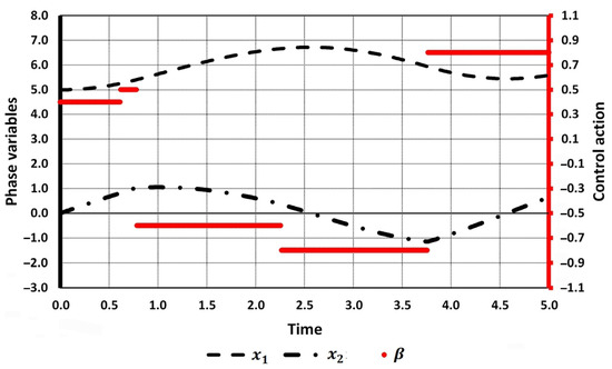
Figure 1.
Initial trajectory and control action (case 2.1).
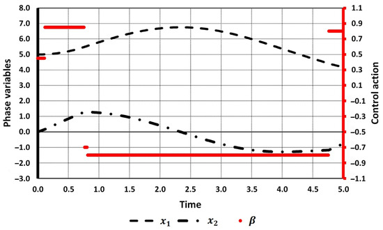
Figure 2.
Initial trajectory and control action (case 2.2).
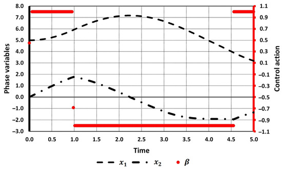
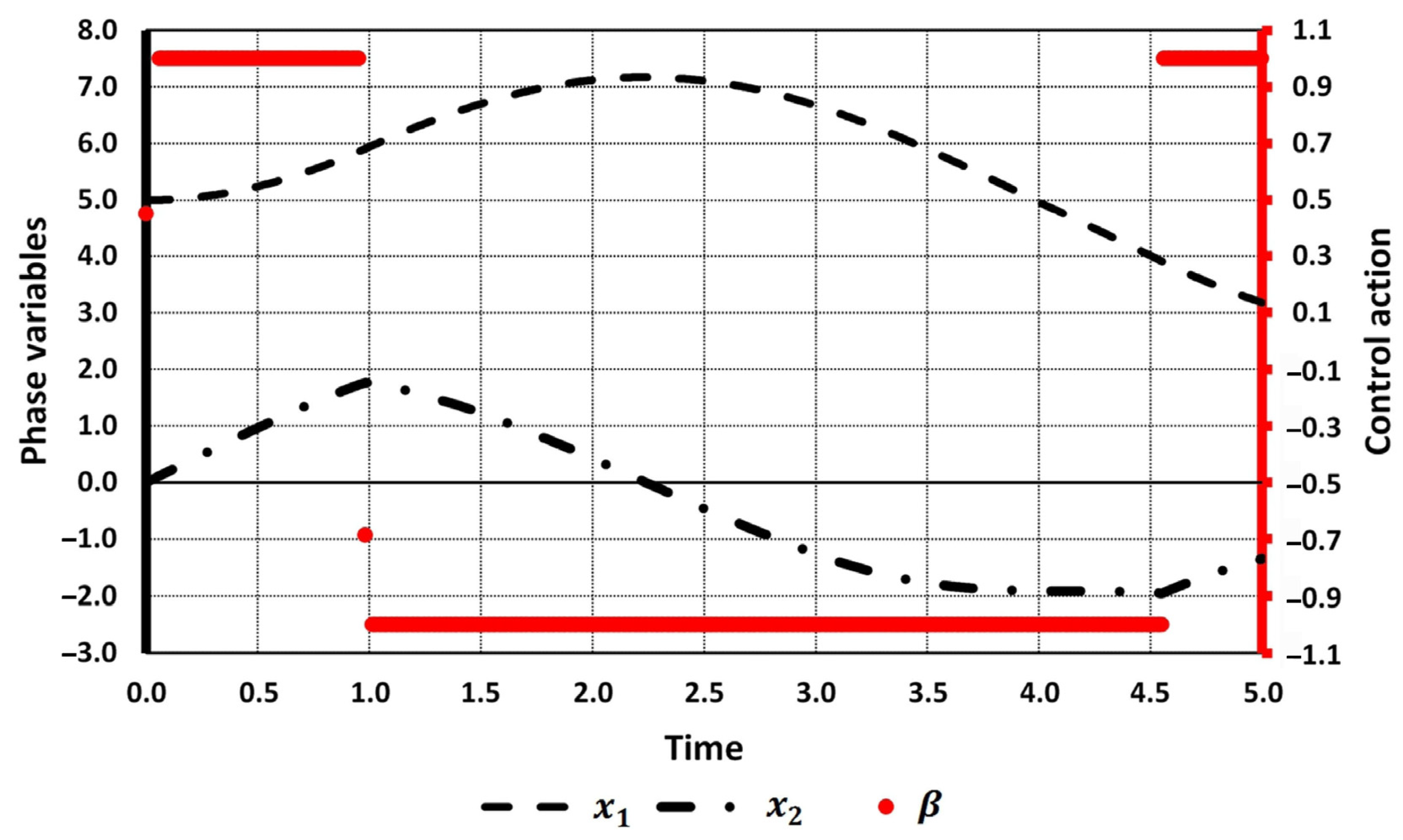
Figure 3.
Optimal trajectory and control action (case 2.2).
Let us analyze the obtained numerical results. When the number of switchings is initially set to two (cases 1.1–1.4), the same solution is obtained for all the guess points.
As for the case of four initial switchings, we have two technically different results. However, using the algorithm proposed in Section 4 for case 2.1, we can merge intervals [0, 0.561] and [0.561, 0.982] because the control action equals 1 at both of them. The same holds for intervals [0.982, 2.156] and [2.156, 4.5]. This results in the solution obtained for cases 1.1–1.4.
Now, let us analyze the solution obtained in case 2.2. The intervals where control actions equal 0.450 and −0.687 are negligibly small (see Figure 3, the control action is linked to the right axis), and they can be removed from consideration. So, the solution obtained in case 2.2 also coincides with that in cases 1.1–1.4.
A comparison with the results provided by first-order methods [27] shows that the second-order method achieves the minimum value of the objective functional, which is less than in [27]. This refinement is the result of the more exact values of the optimal switchings.
6. Conclusions
This paper provides formulas for the use of second-order methods for solving optimal control problems in parametrically specified classes of control actions. In the problem, both the switching times of the control parameters and the parameters themselves are being optimized. Despite the awkwardness of the obtained formulas, their use is efficient when it is necessary to repeatedly solve a specific control problem for different values of the parameters involved in the problem. Such parameters can be the values of the coefficients involved in differential Equation (1) or the values of the initial conditions.
This paper presents the results of numerical experiments and a comparison with the results obtained by first-order optimal control methods, including those given in other works.
Author Contributions
Conceptualization, K.A.-z., A.H. and E.P.; methodology, K.A.-z., A.H. and E.P.; software, K.A.-z.; validation, K.A.-z., A.H. and E.P.; formal analysis, K.A.-z., A.H. and E.P.; writing—original draft preparation, K.A.-z. and A.H.; writing—review and editing E.P. All authors have read and agreed to the published version of the manuscript.
Funding
This research received no external funding.
Data Availability Statement
The original contributions presented in the study are included in the article, further inquiries can be directed to the corresponding author/s.
Acknowledgments
The authors would like to thank the anonymous reviewers for their valuable comments.
Conflicts of Interest
The authors declare no conflicts of interest.
References
- Evtushenko, Y.G.; Tret’yakov, A.A. On the Redundancy of Hessian Nonsingularity for Linear Convergence Rate of the Newton Method Applied to the minimization of Convex Functions. Comput. Math. Math. Phys. 2024, 64, 781–787. [Google Scholar] [CrossRef]
- Evtushenko, Y.G. Numerical Optimization Techniques; Springer: New York, NY, USA, 1985. [Google Scholar]
- Handzel, A.V. Second-order method in network problems. Bull. Natl. Acad. Sci. Azerbaijan Ser. Phys. Eng. Math. 1989, 1, 89–91. (In Russian) [Google Scholar]
- Chicharro, F.I.; Cordero, A.; Garrido, N.; Torregrosa, J.R. Generating Root-Finder Iterative Methods of Second Order: Convergence and Stability. Axioms 2019, 8, 55. [Google Scholar] [CrossRef]
- Torres-Hernandez, A.; Brambila-Paz, F.; Iturrarán-Viveros, U.; Caballero-Cruz, R. Fractional Newton–Raphson Method Accelerated with Aitken’s Method. Axioms 2021, 10, 47. [Google Scholar] [CrossRef]
- Arutyunov, A.V.; Karamzin, D.Y.; Pereira, F.L. Maximum Principle and Second-Order Optimality Conditions in Control Problems with Mixed Constraints. Axioms 2022, 11, 40. [Google Scholar] [CrossRef]
- Providas, E.; Kattis, M. A simple finite element model for the geometrically nonlinear analysis of thin shells. Comput. Mech. 1999, 24, 127–137. [Google Scholar] [CrossRef]
- Ekaterinaris, J.A. High-order accurate, low numerical diffusion methods for aerodynamics. Prog. Aerosp. Sci. 2005, 41, 192–300. [Google Scholar] [CrossRef]
- Wang, Z.J.; Fidkowski, K.; Abgrall, R.; Bassi, F.; Caraeni, D.; Cary, A.; Deconinck, H.; Hartmann, R.; Hillewaert, K.; Huynh, H.T.; et al. High-order CFD methods: Current status and perspective. Int. J. Numer. Meth. Fluids 2013, 72, 811–845. [Google Scholar] [CrossRef]
- Argyros, I.K.; Szidarovszky, F. The Theory and Applications of Iteration Methods; CRC Press: Boca Raton, FL, USA, 1993. [Google Scholar]
- Hinze, M.; Kunisch, K. Second Order Methods for Optimal Control of Time-Dependent Fluid Flow. SIAM J. Control. Optim. 2001, 40, 925–946. [Google Scholar] [CrossRef]
- Kaplan, M.L.; Heegaard, J.H. Second-order optimal control algorithm for complex systems. Int. J. Numer. Meth. Engng. 2002, 53, 2043–2060. [Google Scholar] [CrossRef]
- Providas, E.A. Unified Formulation of Analytical and Numerical Methods for Solving Linear Fredholm Integral Equations. Algorithms 2021, 14, 293. [Google Scholar] [CrossRef]
- Corriou, J.-P. (Ed.) Analytical Methods for Optimization. In Numerical Methods and Optimization: Theory and Practice for Engineers, 1st ed.; Springer: Cham, Switzerland, 2021; pp. 455–503. [Google Scholar]
- Deep, G.; Argyros, I.K.; Verma, G.; Kaur, S.; Kaur, R.; Regmi, S. Extended Higher Order Iterative Method for Nonlinear Equations and its Convergence Analysis in Banach Spaces. Contemp. Math. 2024, 5, 230–254. [Google Scholar] [CrossRef]
- Aida-zade, K.R.; Evtushenko, Y.G. Fast automatic differentiation on a computer. Math. Models Comput. Simul. 1989, 1, 120–131. (In Russian) [Google Scholar]
- Evtushenko, Y.G. Optimization and Fast Automatic Differentiation; Dorodnicyn Computing Centre of Russian Academy of Sciences: Moscow, Russia, 2013. (In Russian) [Google Scholar]
- Aida-zade, K.R.; Talybov, S.G. On consistency of schemes for finite difference approximation of boundary value problems in optimal control. Bull. Natl. Acad. Sci. Azerbaijan Ser. Phys. Eng. Math. 1998, 6, 21–25. (In Russian) [Google Scholar]
- Griewank, A.; Walther, A. Evaluating Derivatives: Principles and Techniques of Algorithmic Differentiation, 2nd ed.; Cambridge University Press: Cambridge, UK, 2008. [Google Scholar]
- Neidinger, R.D. Introduction to Automatic Differentiation and MATLAB Object-Oriented Programming. SIAM Rev. 2010, 52, 545–563. [Google Scholar] [CrossRef]
- Baydin, A.G.; Barak, A.P.; Radul, A.A.; Siskind, J.M. Automatic Differentiation in Machine Learning: A Survey. J. Mach. Learn. Res. 2018, 153, 1–43. [Google Scholar]
- Polak, E. Computational Methods in Optimization: A Unified Approach; Academic Press: New York, USA, 1971. [Google Scholar]
- Li, R.; Teo, K.L.; Wong, K.H.; Duan, G.R. Control parameterization enhancing transform for optimal control of switched systems. Math. Comput. Model. 2006, 1112, 1393–1403. [Google Scholar] [CrossRef]
- Aida-zade, K.R.; Evtushenko, Y.G.; Talybov, S.G. Numerical schemes for solving problems of optimal control of objects with distributed parameters. Bull. Natl. Acad. Sci. Azerbaijan Ser. Phys. Eng. Math. 1985, 5, 34–40. (In Russian) [Google Scholar]
- Aida-zade, K.R. Study and numerical solution of finite difference approximations of distributed-system control problems. Comput. Math. Math. Phys. 1989, 29, 15–21. [Google Scholar] [CrossRef]
- Rahimov, A.B. On an approach to solution to optimal control problems on the classes of piecewise constant, piecewise linear, and piecewise given functions. Tomsk. State Univ. J. Control Comput. Sci. 2012, 19, 20–30. (In Russian) [Google Scholar]
- Aida-zade, K.R.; Ragimov, A.B. Solution of Optimal Control Problem in Class of Piecewise-Constant Functions. Autom. Control. Comput. Sci. 2007, 41, 18–24. [Google Scholar] [CrossRef]
- Vasil’ev, O.V.; Tyatyushkin, A.I. A method for solving optimal control problems based on the maximum principle. Comput. Math. Math. Phys. 1981, 21, 14–22. (In Russian) [Google Scholar] [CrossRef]


Disclaimer/Publisher’s Note: The statements, opinions and data contained in all publications are solely those of the individual author(s) and contributor(s) and not of MDPI and/or the editor(s). MDPI and/or the editor(s) disclaim responsibility for any injury to people or property resulting from any ideas, methods, instructions or products referred to in the content. |
© 2024 by the authors. Licensee MDPI, Basel, Switzerland. This article is an open access article distributed under the terms and conditions of the Creative Commons Attribution (CC BY) license (https://creativecommons.org/licenses/by/4.0/).