Ulam–Hyers Stability and Simulation of a Delayed Fractional Differential Equation with Riemann–Stieltjes Integral Boundary Conditions and Fractional Impulses

Abstract

In this article, we delve into delayed fractional differential equations with Riemann–Stieltjes integral boundary conditions and fractional impulses. By using differential inequality techniques and some fixed-point theorems, some novel sufficient assessments for convenient verification have been devised to ensure the existence and uniqueness of solutions. We further employ the nonlinear analysis to reveal that this problem is Ulam–Hyers (UH) stable. Finally, some examples and numerical simulations are presented to illustrate the reliability and validity of our main results.

1. Introduction

Fractional calculus is a generalization of the traditional integer-order calculus to an arbitrary real order. The earliest exploration of fractional derivatives dates back to a correspondence between L’Hospital and Leibnitz in 1695. In the 1970s, it was discovered that fractal geometry, the memory process, the power-law phenomenon and the genetic phenomenon are closely related to fractional derivatives. Fractional derivatives are excellent instruments for memory and genetic processes. Concurrently, due to the widespread application of fractional differential equations in disciplines such as physics, chemistry, aerodynamics, complex dielectric electrodynamics, polymer rheology, capacitor theory, circuits, biology and control theory (see [1,2,3,4,5,6]), they have received increasing attention and focus. As a consequence, many articles on fractional-order differential equations have been published to explore the existence, uniqueness and multiplicity of solutions by using Green’s function and related fixed-point theorems. One can see [7,8,9,10,11,12,13,14,15,16,17] and references therein.

Since the last century, some researchers have begun to apply impulsive differential equations to depict sudden events such as diseases, food shortages, natural disasters, etc., in population dynamics systems. Recently, impulsive fractional differential equations have been widely applied in physics and social sciences. The impulsive effect makes the study of fractional differential systems more complex and challenging. Specifically, the impulsive term has affected the dynamic behavior of the system (see [17,18,19]). Meanwhile, the integral boundary value problem (IBVP) for fractional differential systems has been widely used in modern scientific and technological applications such as groundwater flow, chemical engineering, thermoelasticity, population dynamics, etc. Many scholars have studied the IBVP for fractional differential systems and obtained many excellent conclusions (see [7,8,9,20]).

In the process of information transmission between different nodes in brain neural networks, internet and information networks, due to the influence of transmission speed, transmission medium and other factors, the information cannot arrive in time, and there is always a certain time delay which is inevitable. In many cases, a small time delay can lead to great changes in the dynamic behavior of the system [7,8,21]. So, we need to consider the effect of time delay on fractional differential models. In addition, stability is crucial for a differential system with practical application settings. Many definitions of stability have been proposed based on actual needs. In 1940s, Hyers and Ulam [22,23] defined a new type of stability i.e., Ulam–Hyers (UH) stability. Subsequently, this concept of stability was promoted as a generalized UH-type, Ulam–Hyers–Rassias (UHR)-type and generalized UHR-type. Some scholars have conducted systematic research on UH-type stability and published corresponding survey papers and monographs (see [24,25,26,27,28]). In the past decade, the UH-type stability of fractional-order systems has been heavily researched, and many excellent results have been obtained (see [29,30,31,32,33,34,35,36]). Nevertheless, the UH-type stability of delayed fractional differential systems with fractional impulses has been rarely studied, as it is much more difficult to investigate than fractional differential equations with integer-order impulses. Accordingly, it is interesting and challenging to explore the Riemann–Stieltjes IBVP for delayed fractional differential systems with fractional impulses.

Motivated by the above arguments, this article emphasizes the following Riemann–Stieltjes IBVP for a delayed fractional-order system with fractional pulses

$$\begin{array}{c}\hfill \left\{\begin{array}{c}{}^c\mathcal{D}_{0^{+}}^{q}u\left(t\right)+f(t,u_t,u^{\prime }\left(t\right),{}^c\mathcal{D}_{0^{+}}^{p}u\left(t\right))=0,t\in J=[0,1],t\ne t_k,\hfill \\ {}^c\mathcal{D}_{0^{+}}^{p}u\left(t_k^{+}\right)-{}^c\mathcal{D}_{0^{+}}^{p}u\left(t_k^{-}\right)=I_k\left(u\left(t_k\right)\right),k=1,2,\dots ,m,\hfill \\ \alpha u\left(0\right)-\beta u^{\prime }\left(0\right)={\int }_0^1{h}_1(s,u\left(s\right))d{A}_1\left(s\right),\hfill \\ \gamma u\left(1\right)+\delta \left({}^c\mathcal{D}_{0^{+}}^{\sigma }u\right)\left(1\right)={\int }_0^1{h}_2(s,u\left(s\right))d{A}_2\left(s\right),\hfill \\ u^{\prime \prime }\left(0\right)=0,\hfill \end{array}\right.\end{array}$$

(1)

subject to the initial function

$$\begin{array}{c}\hfill u\left(s\right)=\xi \left(s\right),s\in [-\tau ,0],\end{array}$$

(2)

where $\alpha ,\beta ,\gamma ,\delta \ge 0$, $2<q\le 3$ and $0<p$, $\sigma <1$. ${}^c\mathcal{D}_{0^{+}}^q$,${}^c\mathcal{D}_{0^{+}}^p$ and ${}^c\mathcal{D}_{0^{+}}^{\sigma }$ express $q,p,\sigma$-order Caputo derivatives. $f\in C(J\times {\mathbb{R}}^3,\mathbb{R})$, $h_i\in C(J\times \mathbb{R},{\mathbb{R}}^{+})(i=1,2)$, $I_k\in C(\mathbb{R},\mathbb{R})(k=1,2,\cdots ,m)$, $0=t_0<t_1<\cdots <t_m<t_{m+1}=1$. Both the left and right limits ${}^c\mathcal{D}_{0^{+}}^{p}u\left(t_k^{-}\right)$ and ${}^c\mathcal{D}_{0^{+}}^{p}u\left(t_k^{+}\right)$ exist, and ${}^c\mathcal{D}_{0^{+}}^{p}u\left(t_k^{-}\right)={}^c\mathcal{D}_{0^{+}}^{p}u\left(t_k\right)$. $A_i:J\to \mathbb{R}(i=1,2)$ indicates the increasing bounded variation. ${\int }_0^1{h}_i(s,u\left(s\right))d{A}_i\left(s\right)(i=1,2)$ denotes the Riemann–Stieltjes integrals. $\mathbb{R}=(-\infty ,+\infty )$, ${\mathbb{R}}^{+}=[0,+\infty )$. $\tau >0$ means the constant lag, $\xi \left(t\right)\in C_{\tau }$ ($C_{\tau }$ defined as Section 3), $u_t\in C_{\tau }$, $u_t\left(\theta \right)=u(t+\theta )$, $\theta \in [-\tau ,0]$.

The main objective of the article is to consider the existence and UH stability for IBVPs (1) and (2). The contribution of this article is mainly reflected in three aspects. (a) Since there are few studies on the Riemann–Stieltjes IBVP for the delayed fractional system with fractional pulses, this study of IBVPs (1) and (2) is the first to fill this gap. (b) We derive the existence, uniqueness and UH stability of IBVPs (1) and (2). (c) We use the appropriate ODE toolbox in MATLAB to obtain the numerical solution and simulation of IBVPs (1) and (2).

The remaining parts of this paper are organized as follows. Section 2 mainly introduces some essential notions, lemmas and the properties of the integral function. Section 3 presents the existence and uniqueness of the solution for IBVPs (1) and (2) by applying differential inequality techniques and some fixed-point theorems. The UH stability of IBVPs (1) and (2) are assessed in Section 4. Some interesting examples and simulations are presented to illustrate the correctness and availability of the main findings in Section 5. A brief summary is provided in Section 6.

2. Preliminaries

In this section, we introduce some necessary definitions and lemmas, which can be found in [37,38,39].

Definition 1

([37]). The Riemann–Liouville fractional integral of order $\alpha >0$ of a function $u:(a,+\infty )\to \mathbb{R}$ is given by

$$\begin{array}{c}\hfill {\mathcal{J}}_{a^{+}}^{\alpha }u\left(t\right)={\displaystyle \frac{1}{\Gamma \left(\alpha \right)}}{\int }_a^t{(t-s)}^{\alpha -1}u\left(s\right)ds,\end{array}$$

provided that the right-hand side is point-wise defined on $(a,+\infty )$.

Definition 2

([37]). If $u\in C^n((a,+\infty ),\mathbb{R})$ and $\alpha >0$, then the Caputo fractional derivative of order α is defined as

$$\begin{array}{c}\hfill {}^c\mathcal{D}_{a^{+}}^{\alpha }u\left(t\right)={\displaystyle \frac{1}{\Gamma (n-\alpha )}}{\int }_a^t{(t-s)}^{n-\alpha -1}{u}^{\left(n\right)}\left(s\right)ds,\end{array}$$

where $n-1<\alpha ⩽n$, provided that the right-hand side is point-wise defined on $(a,+\infty )$.

Lemma 1

([38]). Assume that $u\in C(0,1)\cap L(0,1)$ with a Caputo fractional derivative of order $\alpha >0$ that belongs to $u\in C^n[0,1]$, then

$$\begin{array}{c}\hfill {\mathcal{J}}_{0^{+}}^{\alpha }{}^c\mathcal{D}_{0^{+}}^{\alpha }u\left(t\right)=u\left(t\right)+d_1+d_{2}t+\cdots +d_n{t}^{n-1},\end{array}$$

for some $d_i\in \mathbb{R},i=1,2,\cdots ,n$, where n satisfies $n-1<\alpha \le n$.

Lemma 2

([38]). If $\alpha ,\beta >0$, $t\in [a,b]$ and $u\left(t\right)\in L[a,b]$, then

$$\begin{array}{c}\hfill {}^c\mathcal{D}_{a^{+}}^{\alpha }{\mathcal{J}}_{a^{+}}^{\alpha }u\left(t\right)=u\left(t\right),{\mathcal{J}}_{a^{+}}^{\alpha }{\mathcal{J}}_{a^{+}}^{\beta }u\left(t\right)={\mathcal{J}}_{a^{+}}^{\alpha +\beta }u\left(t\right).\end{array}$$

Lemma 3

([39]). Let $\mathbb{X}$ be a Banach space and Ω be a closed convex subset of $\mathbb{X}$. If the operator $\mathcal{L}:\overline{\Omega }\to \overline{\Omega }$ is completely continuous, then the operator $\mathcal{L}$ has at least one fixed point $u^{*}\in \overline{\Omega }$.

Lemma 4

([39]). Given a Banach space $\mathbb{X}$, let $\mathbb{E}\ne \varnothing$ be a closed subset of $\mathbb{X}$. If the operator $\mathcal{F}:\mathbb{E}\to \mathbb{E}$ is contractive, then there is a unique $u^{*}\in \mathbb{E}$ such that $\mathcal{F}{u}^{*}=u^{*}$.

Consider the following fractional-order impulsive boundary value problem and impulsive integral equation:

$$\begin{array}{c}\hfill \left\{\begin{array}{c}{}^c\mathcal{D}_{0^{+}}^{q}u\left(t\right)+f\left(t\right)=0,t\in J:=[0,1],t\ne t_k,2<q\le 3,\hfill \\ {}^c\mathcal{D}_{0^{+}}^{p}u\left(t_k^{+}\right)-{}^c\mathcal{D}_{0^{+}}^{p}u\left(t_k^{-}\right)=I_k\left(x\left(t_k\right)\right),k=1,2,\dots ,m,0<p<1,\hfill \\ \alpha u\left(0\right)-\beta u^{\prime }\left(0\right)={\int }_0^1{h}_1(s,u\left(s\right))d{A}_1\left(s\right),\alpha ,\beta \ge 0,\hfill \\ \gamma u\left(1\right)+\delta \left({}^c\mathcal{D}_{0^{+}}^{\sigma }u\right)\left(1\right)={\int }_0^1{h}_2(s,u\left(s\right))d{A}_2\left(s\right),0<\sigma <1,\gamma ,\delta \ge 0,\hfill \\ u^{\prime \prime }\left(0\right)=0,\hfill \end{array}\right.\end{array}$$

(3)

and

$$\begin{array}{cc}\hfill u\left(t\right)=& {\int }_0^{1}G(t,s)f\left(s\right)ds+{\displaystyle \frac{1}{{\Delta }_1}}\left[(1-t)\gamma +{\displaystyle \frac{\delta }{\Gamma (2-\sigma )}}\right]{\int }_0^1{h}_1(s,u\left(s\right))d{A}_1\left(s\right)\hfill \\ \hfill & +{\displaystyle \frac{\beta +\alpha t}{{\Delta }_1}}{\int }_0^1{h}_2(s,u\left(s\right))d{A}_2\left(s\right)\hfill \\ \hfill & -\Gamma (2-p){\displaystyle \frac{\beta +\alpha t}{{\Delta }_1}}\left[(\gamma +{\displaystyle \frac{\delta }{\Gamma (2-\sigma )}})\sum _{j=1}^m{t}_j^{p-1}{I}_j\left(u\left(t_j\right)\right)-\gamma \sum _{j=1}^m{t}_j^p{I}_j\left(u\left(t_j\right)\right)\right]\hfill \\ \hfill & +\Gamma (2-p)\sum _{j=1}^k{t}_j^{p-1}(t-t_j)I_j\left(u\left(t_j\right)\right),t\in (t_k,t_{k+1}],k=1,2,\dots ,m,\hfill \end{array}$$

(4)

where

$$\begin{array}{c}\hfill {\Delta }_1=\left|\begin{array}{cc}\alpha \hfill & -\beta \hfill \\ \gamma \hfill & \gamma +{\displaystyle \frac{\delta }{\Gamma (2-\sigma )}}\hfill \end{array}\right|=(\alpha +\beta )\gamma +{\displaystyle \frac{\alpha \delta }{\Gamma (2-\sigma )}},\end{array}$$

(5)

$$\begin{array}{c}\hfill G(t,s)=\left\{\begin{array}{c}-{\displaystyle \frac{{(t-s)}^{q-1}}{\Gamma \left(q\right)}}+g_1(t,s),0\le s\le t\le 1,\hfill \\ g_1(t,s),0\le t\le s\le 1,\hfill \end{array}\right.\end{array}$$

(6)

and

$$\begin{array}{c}\hfill g_1(t,s)={\displaystyle \frac{\beta +\alpha t}{{\Delta }_1}}\left[{\displaystyle \frac{\gamma }{\Gamma \left(q\right)}}{(1-s)}^{q-1}+{\displaystyle \frac{\delta }{\Gamma (q-\sigma )}}{(1-s)}^{q-\sigma -1}\right].\end{array}$$

Lemma 5.

Let $f\in C(J,\mathbb{R})$ and ${\Delta }_1\ne 0$. Then, a function $u\in C((t_k,t_{k+1}],\mathbb{R})$ solves the IBVP (3) iff $u\in C((t_k,t_{k+1}],\mathbb{R})$ solves the Equation (4)

Proof. 

When $t\in [0,t_1]$, from Lemma 1 and system (3), we obtain

$$\begin{array}{c}\hfill u\left(t\right)=-{\mathcal{J}}_{0^{+}}^{q}f\left(t\right)+c_{10}+c_{11}t+c_{12}{t}^2.\end{array}$$

(7)

It follows from (7) that $u\left(0\right)=c_{10}$, and

$$\begin{array}{c}\hfill u^{\prime }\left(t\right)=-{\displaystyle \frac{1}{\Gamma (q-1)}}{\int }_0^t{(t-s)}^{q-2}f\left(s\right)ds+c_{11}+2c_{12}t.\end{array}$$

(8)

From (8), we derive that $u^{\prime }\left(0\right)=c_{11}$ and $u^{\prime \prime }\left(0\right)=0$, which implies that $c_{12}=0$.

In the light of the integral boundary value condition of system (3), we have

$$\begin{array}{c}\hfill \alpha c_{10}-\beta c_{11}={\int }_0^1{h}_1(s,u\left(s\right))d{A}_1\left(s\right).\end{array}$$

(9)

By Lemma 2 and (7), one yields that

$$\begin{array}{c}\hfill {}^c\mathcal{D}_{0^{+}}^{p}u\left(t\right)=-{\mathcal{J}}_{0^{+}}^{q-p}f\left(t\right)+{\displaystyle \frac{c_{11}}{\Gamma (2-p)}}{t}^{1-p},\end{array}$$

(10)

and

$$\begin{array}{c}\hfill {}^c\mathcal{D}_{0^{+}}^{p}u\left(t_1^{-}\right)=-{\mathcal{J}}_{0^{+}}^{q-p}f\left(t_1\right)+{\displaystyle \frac{c_{11}}{\Gamma (2-p)}}{t}_1^{1-p}.\end{array}$$

(11)

When $t\in (t_1,t_2]$, we similarly have

$$\begin{array}{c}\hfill u\left(t\right)=-{\mathcal{J}}_{0^{+}}^{q}f\left(t\right)+c_{20}+c_{21}t,\end{array}$$

(12)

$$\begin{array}{c}\hfill {}^c\mathcal{D}_{0^{+}}^{p}u\left(t\right)=-{\mathcal{J}}_{0^{+}}^{q-p}f\left(t\right)+{\displaystyle \frac{c_{21}}{\Gamma (2-p)}}{t}^{1-p}.\end{array}$$

(13)

From (7) and (12), we know that

$$\begin{array}{c}\hfill u\left(t_1^{-}\right)=-{\mathcal{J}}_{0^{+}}^{q}f\left(t_1\right)+c_{10}+c_{11}{t}_1,\end{array}$$

and

$$\begin{array}{c}\hfill u\left(t_1^{+}\right)=-{\mathcal{J}}_{0^{+}}^{q}f\left(t_1\right)+c_{20}+c_{21}{t}_1.\end{array}$$

In view of the continuity of $u\left(t\right)$ at $t_1$, we obtain

$$\begin{array}{c}\hfill c_{10}-c_{20}=(c_{21}-c_{11})t_1.\end{array}$$

(14)

From (13), we have

$$\begin{array}{c}\hfill {}^c\mathcal{D}_{0^{+}}^{p}u\left(t_1^{+}\right)=-{\mathcal{J}}_{0^{+}}^{q-p}f\left(t_1\right)+{\displaystyle \frac{c_{21}}{\Gamma (2-p)}}{t}_1^{1-p}.\end{array}$$

(15)

By (11), (15) and ${}^c\mathcal{D}_{0^{+}}^{p}u\left(t_1^{+}\right)-{}^c\mathcal{D}_{0^{+}}^{p}u\left(t_1^{-}\right)=I_1\left(u\left(t_1\right)\right)$, one has

$$\begin{array}{c}\hfill c_{21}-c_{11}=\Gamma (2-p)t_1^{p-1}{I}_1\left(u\left(t_1\right)\right).\end{array}$$

(16)

Similarly, when $t\in (t_k,t_{k+1}]$, $2\le k\le m-1$, we obtain

$$\begin{array}{c}\hfill c_{k0}-c_{k+1,0}=(c_{k+1,1}-c_{k1})t_k,\end{array}$$

(17)

and

$$\begin{array}{c}\hfill c_{k+1,1}-c_{k1}=\Gamma (2-p)t_k^{p-1}{I}_k\left(u\left(t_k\right)\right).\end{array}$$

(18)

From (16)–(18), we obtain

$$\begin{array}{c}\hfill c_{k+1,1}-c_{11}=\Gamma (2-p)\sum _{j=1}^k{t}_j^{p-1}{I}_j\left(u\left(t_j\right)\right),\end{array}$$

(19)

and

$$\begin{array}{c}\hfill c_{10}-c_{k+1,0}=\Gamma (2-p)\sum _{j=1}^k{t}_j^p{I}_j\left(u\left(t_j\right)\right).\end{array}$$

(20)

Next, let $t_{m+1}=1$. When $t\in (t_m,t_{m+1}]$, one derives that

$$\begin{array}{c}\hfill u\left(t\right)=-{\mathcal{J}}_{0^{+}}^{q}f\left(t\right)+c_{m+1,0}+c_{m+1,1}t.\end{array}$$

(21)

Similarly,

$$\begin{array}{c}\hfill c_{m+1,0}=c_{10}-\Gamma (2-p)\sum _{j=1}^m{t}_j^p{I}_j\left(u\left(t_j\right)\right),\end{array}$$

(22)

and

$$\begin{array}{c}\hfill c_{m+1,1}=c_{11}+\Gamma (2-p)\sum _{j=1}^m{t}_j^{p-1}{I}_j\left(u\left(t_j\right)\right).\end{array}$$

(23)

From (21)–(23), when $t\in (t_m,t_{m+1}]$, one has

$$\begin{array}{c}\hfill u\left(t\right)=-{\mathcal{J}}_{0^{+}}^{q}f\left(t\right)+c_{10}+c_{11}t+\Gamma (2-p)\sum _{j=1}^m{t}_j^{p-1}(t-t_j)I_j\left(u\left(t_j\right)\right).\end{array}$$

(24)

So,

$$\begin{array}{c}\hfill u\left(1\right)=-{\mathcal{J}}_{0^{+}}^{q}f\left(1\right)+c_{10}+c_{11}+\Gamma (2-p)\sum _{j=1}^m{t}_j^{p-1}(1-t_j)I_j\left(u\left(t_j\right)\right),\end{array}$$

(25)

$$\begin{array}{c}\hfill {}^c\mathcal{D}_{0^{+}}^{\sigma }u\left(t\right)=-{\mathcal{J}}_{0^{+}}^{q-\sigma }f\left(t\right)+c_{m+1,1}{\displaystyle \frac{t^{1-\sigma }}{\Gamma (2-\sigma )}},\end{array}$$

(26)

and

$$\begin{array}{c}\hfill \left({}^c\mathcal{D}_{0^{+}}^{\sigma }u\left(t\right)\right)\left(1\right)=-{\mathcal{J}}_{0^{+}}^{q-\sigma }f\left(1\right)+{\displaystyle \frac{c_{11}}{\Gamma (2-\sigma )}}+{\displaystyle \frac{\Gamma (2-p)}{\Gamma (2-\sigma )}}\sum _{j=1}^m{t}_j^{p-1}{I}_j\left(u\left(t_j\right)\right).\end{array}$$

(27)

Using $\gamma u\left(1\right)+\delta \left({}^c\mathcal{D}_{0^{+}}^{\sigma }u\right)\left(1\right)={\int }_0^1{h}_2(s,u\left(s\right))d{A}_2\left(s\right)$, (25) and (27), we derive that

$$\begin{array}{cc}\hfill \gamma c_{10}+(\gamma +{\displaystyle \frac{\delta }{\Gamma (2-\sigma )}})c_{11}=& \gamma {\mathcal{J}}_{0^{+}}^{q}f\left(1\right)+\delta {\mathcal{J}}_{0^{+}}^{q-\delta }f\left(1\right)+\gamma \Gamma (2-p)\sum _{j=1}^m{t}_j^{p-1}(t_j-1)I_j\left(u\left(t_j\right)\right)\hfill \\ \hfill & -{\displaystyle \frac{\delta \Gamma (2-p)}{\Gamma (2-\sigma )}}\sum _{j=1}^m{t}_j^{p-1}{I}_j\left(u\left(t_j\right)\right)+{\int }_0^1{h}_2(s,u\left(s\right))d{A}_2\left(s\right).\hfill \end{array}$$

(28)

From (9) and (28), we obtain

$$\begin{array}{cc}\hfill c_{10}=& {\displaystyle \frac{1}{{\Delta }_1}}\left|\begin{array}{cc}{\int }_0^1{h}_1(s,u\left(s\right))d{A}_1\left(s\right)& -\beta \\ \varsigma +{\int }_0^1{h}_2(s,u\left(s\right))d{A}_2\left(s\right)& \gamma +{\displaystyle \frac{\delta }{\Gamma (2-\sigma )}}\end{array}\right|\hfill \\ \hfill =& {\displaystyle \frac{1}{{\Delta }_1}}\left[(r+{\displaystyle \frac{\delta }{\Gamma (2-\sigma )}}){\int }_0^1{h}_1(s,u\left(s\right))d{A}_1\left(s\right)+\beta \varsigma +\beta {\int }_0^1{h}_2(s,u\left(s\right))d{A}_2\left(s\right)\right],\hfill \end{array}$$

(29)

where

$$\begin{array}{cc}\hfill \varsigma =& \gamma {\mathcal{J}}_{0^{+}}^{q}f\left(1\right)+\delta {\mathcal{J}}_{0^{+}}^{q-\delta }f\left(1\right)+\gamma \Gamma (2-p)\sum _{j=1}^m{t}_j^{p-1}(t_j-1)I_j\left(u\left(t_j\right)\right)\hfill \\ \hfill & -{\displaystyle \frac{\delta \Gamma (2-p)}{\Gamma (2-\sigma )}}\sum _{j=1}^m{t}_j^{p-1}{I}_j\left(u\left(t_j\right)\right).\hfill \end{array}$$

(30)

From (9), we obtain

$$\begin{array}{c}\hfill c_{11}={\displaystyle \frac{\alpha c_{10}-{\int }_0^{1}h(s,u\left(s\right))d{A}_1\left(s\right)}{\beta }}.\end{array}$$

(31)

Therefore, $\forall t\in (t_k,t_{k+1}]$, $0\le k\le m$, one obtains

$$\begin{array}{cc}\hfill u\left(t\right)=& -{\mathcal{J}}_{0^{+}}^{q}f\left(t\right)+c_{k+1,0}+c_{k+1,1}t\hfill \\ \hfill =& -{\mathcal{J}}_{0^{+}}^{q}f\left(t\right)+(1+{\displaystyle \frac{\alpha }{\beta }}t)c_{10}-{\displaystyle \frac{t}{\beta }}{\int }_0^1{h}_1(s,u\left(s\right))d{A}_1\left(s\right)+\Gamma (2-p)\sum _{j=1}^k{t}_j^{p-1}(t-t_j)I_j\left(u\left(t_j\right)\right)\hfill \\ \hfill =& -{\mathcal{J}}_{0^{+}}^{q}f\left(t\right)+{\displaystyle \frac{\gamma }{{\Delta }_1}}(\beta +\alpha t){\mathcal{J}}_{0^{+}}^{q}f\left(1\right)+{\displaystyle \frac{\delta }{{\Delta }_1}}(\beta +\alpha t){\mathcal{J}}_{0^{+}}^{q-\sigma }f\left(1\right)\hfill \\ \hfill & +{\displaystyle \frac{1}{{\Delta }_1}}[(1-t)\gamma +{\displaystyle \frac{\delta }{\Gamma (2-\sigma )}}]{\int }_0^1{h}_1(s,u\left(s\right))d{A}_1\left(s\right)+{\displaystyle \frac{1}{{\Delta }_1}}(\beta +\alpha t){\int }_0^1{h}_2(s,u\left(s\right))d{A}_2\left(s\right)\hfill \\ \hfill & -{\displaystyle \frac{1}{{\Delta }_1}}\Gamma (2-p)(\gamma +{\displaystyle \frac{\delta }{\Gamma (2-\sigma )}})(\beta +\alpha t)\sum _{j=1}^m{t}_j^{p-1}{I}_j\left(u\left(t_j\right)\right)\hfill \\ \hfill & +{\displaystyle \frac{\gamma }{{\Delta }_1}}\Gamma (2-p)(\beta +\alpha t)\sum _{j=1}^m{t}_j^p{I}_j\left(u\left(t_j\right)\right)+\Gamma (2-p)\sum _{j=1}^k{t}_j^{p-1}(t-t_j)I_j\left(u\left(t_j\right)\right)\hfill \end{array}$$

$$\begin{array}{cc}\hfill =& {\int }_0^{1}G(t,s)f\left(s\right)ds+{\displaystyle \frac{1}{{\Delta }_1}}[(1-t)\gamma +{\displaystyle \frac{\delta }{\Gamma (2-\sigma )}}]{\int }_0^1{h}_1(s,u\left(s\right))d{A}_1\left(s\right)\hfill \\ \hfill & +{\displaystyle \frac{\beta +\alpha t}{{\Delta }_1}}{\int }_0^1{h}_2(s,u\left(s\right))d{A}_2\left(s\right)\hfill \\ \hfill & -\Gamma (2-p){\displaystyle \frac{\beta +\alpha t}{{\Delta }_1}}\left[(\gamma +{\displaystyle \frac{\delta }{\Gamma (2-\sigma )}})\sum _{j=1}^m{t}_j^{p-1}{I}_j\left(u\left(t_j\right)\right)-\gamma \sum _{j=1}^m{t}_j^p{I}_j\left(u\left(t_j\right)\right)\right]\hfill \\ \hfill & +\Gamma (2-p)\sum _{j=1}^k{t}_j^{p-1}(t-t_j)I_j\left(u\left(t_j\right)\right).\hfill \end{array}$$

The proof ends. □

Lemma 6.

Let $\alpha ,\beta ,\gamma ,\delta \ge 0$, $2<q\le 3$ and $0<\sigma <1$. Then, $G(t,s)$ defined by (6) is continuous and differentiable, and satisfies the following properties

(i)

${\int }_0^1\left|G(t,s)\right|ds⩽{\displaystyle \frac{1}{\Gamma (q+1)}}+{\displaystyle \frac{\beta +\alpha }{{\Delta }_1}}\left[{\displaystyle \frac{\gamma }{\Gamma (q+1)}}+{\displaystyle \frac{\delta }{\Gamma (q-\sigma +1)}}\right]$, $\forall (t,s)\in [0,1]\times [0,1]$.

(ii)

${\int }_0^1\left|{\displaystyle \frac{\partial G}{\partial t}}\right|ds⩽{\displaystyle \frac{1}{\Gamma \left(q\right)}}+{\displaystyle \frac{\alpha }{{\Delta }_1}}\left[{\displaystyle \frac{\gamma }{\Gamma (q+1)}}+{\displaystyle \frac{\delta }{\Gamma (q-\sigma +1)}}\right]$, $\forall (t,s)\in [0,1]\times [0,1]$.

(iii)

${\int }_0^1\left|{\displaystyle \frac{{\partial }^{2}G}{\partial t^2}}\right|ds⩽{\displaystyle \frac{1}{\Gamma (q-1)}}$, $\forall (t,s)\in [0,1]\times [0,1]$.

Proof. 

From the expression of $G(t,s)$, we obtain

$$\begin{array}{cc}\hfill {\int }_0^1\left|G(t,s)\right|ds⩽& {\displaystyle \frac{1}{\Gamma \left(q\right)}}{\int }_0^t{(t-s)}^{q-1}ds+{\displaystyle \frac{1}{\Gamma \left(q\right)}}{\displaystyle \frac{\gamma }{{\Delta }_1}}(\beta +\alpha ){\int }_0^1{(1-s)}^{q-1}ds\hfill \\ \hfill & +{\displaystyle \frac{1}{\Gamma (q-\sigma )}}{\displaystyle \frac{\delta }{{\Delta }_1}}(\beta +\alpha ){\int }_0^1{(1-s)}^{q-\sigma -1}ds\hfill \\ \hfill ⩽& {\displaystyle \frac{1}{\Gamma (q+1)}}+{\displaystyle \frac{\beta +\alpha }{{\Delta }_1}}\left[{\displaystyle \frac{\gamma }{\Gamma (q+1)}}+{\displaystyle \frac{\delta }{\Gamma (q-\sigma +1)}}\right],\hfill \end{array}$$

$$\begin{array}{c}\hfill {\displaystyle \frac{\partial G(t,s)}{\partial t}}=\left\{\begin{array}{cc}-{\displaystyle \frac{{(t-s)}^{q-2}}{\Gamma (q-1)}}+{\displaystyle \frac{\alpha }{{\Delta }_1}}\left[{\displaystyle \frac{\gamma }{\Gamma \left(q\right)}}{(1-s)}^{q-1}+{\displaystyle \frac{\delta }{\Gamma (q-\sigma )}}{(1-s)}^{q-\sigma -1}\right],\hfill & 0⩽s⩽t⩽1,\hfill \\ {\displaystyle \frac{\alpha }{{\Delta }_1}}\left[{\displaystyle \frac{\gamma }{\Gamma \left(q\right)}}{(1-s)}^{q-1}+{\displaystyle \frac{\delta }{\Gamma (q-\sigma )}}{(1-s)}^{q-\sigma -1}\right],\hfill & 0⩽t⩽s⩽1,\hfill \end{array}\right.\end{array}$$

and

$$\begin{array}{c}\hfill {\displaystyle \frac{{\partial }^{2}G(t,s)}{\partial t^2}}=\left\{\begin{array}{cc}-{\displaystyle \frac{{(t-s)}^{q-3}}{\Gamma (q-2)}},\hfill & 0⩽s⩽t⩽1,\hfill \\ 0,\hfill & 0⩽t⩽s⩽1.\hfill \end{array}\right.\end{array}$$

By simple calculation, we have

$$\begin{array}{cc}\hfill {\int }_0^1\left|{\displaystyle \frac{\partial G}{\partial t}}\right|ds⩽& {\displaystyle \frac{1}{\Gamma \left(q\right)}}+{\displaystyle \frac{\alpha }{{\Delta }_1}}\left[{\displaystyle \frac{\gamma }{\Gamma (q+1)}}+{\displaystyle \frac{\delta }{\Gamma (q-\sigma +1)}}\right],\hfill \end{array}$$

and

$$\begin{array}{c}\hfill {\int }_0^1\left|{\displaystyle \frac{{\partial }^{2}G}{\partial t^2}}\right|ds⩽{\displaystyle \frac{1}{\Gamma (q-2)}}{\int }_0^t{(t-s)}^{q-3}ds⩽{\displaystyle \frac{1}{\Gamma (q-1)}}.\end{array}$$

The proof ends. □

3. Existence Results

This portion focuses on the solvability of IBVPs (1) and (2). To this end, we need to introduce some useful Banach spaces.

For $\tau >0$, a Banach space is defined as $C_{\tau }=\{\xi :\xi ,{\xi }^{\prime },{}^c\mathcal{D}_{0^{+}}^p\xi \in C([-\tau ,0],\mathbb{R})\}$ and its norm as

$$\begin{array}{c}\hfill {\left|\right|\xi \left|\right|}_{[-\tau ,0]}=\underset{-\tau ⩽s⩽0}{sup}\left\{\left|\xi \left(s\right)\right|,|{\xi }^{\prime }{\left(s\right)|,|}^c{\mathcal{D}}_{0^{+}}^p\xi \left(s\right)|\right\}.\end{array}$$

Let $I=[-\tau ,1]$. Then, the set $C(I,\mathbb{R})$ composed of all continuous functions $u:I\to \mathbb{R}$ and the supremum norm ${\displaystyle {\parallel u\parallel }_C=\underset{t\in I}{sup}\left|u\left(t\right)\right|}$ form a Banach space.

The function space $\mathbb{X}=P{C}^1(I,\mathbb{R})$ is defined by

$$\begin{array}{cc}\hfill P{C}^1(I,\mathbb{R})=& \{u\left(t\right)\in C(I,\mathbb{R}):{}^c\mathcal{D}_{0^{+}}^{p}u\left(t\right)\in C((t_{k-1},t_k],\mathbb{R}),{}^c\mathcal{D}_{0^{+}}^{p}u\left(t_k^{+}\right)\mathrm{and}{}^c\mathcal{D}_{0^{+}}^{p}u\left(t_k^{-}\right)\hfill \\ \hfill & \mathrm{all}\mathrm{exist},{}^c\mathcal{D}_{0^{+}}^{p}u\left(t_k^{-}\right)={}^c\mathcal{D}_{0^{+}}^{p}u\left(t_k\right),0<p<1,1⩽k⩽m+1\},\hfill \end{array}$$

and the norm

$$\begin{array}{c}\hfill {\left|\right|u\left|\right|}_{P{C}^1}=max\left\{{\left|\right|u\left|\right|}_C,\left|\right|u^{\prime }{\left|\right|}_C,||{}^c\mathcal{D}_{0^{+}}^{p}u\left(s\right){\left|\right|}_C\right\},\forall u\in P{C}^1(I,\mathbb{R}),\end{array}$$

then, it is obvious that $(P{C}^1(I,\mathbb{R}),\parallel ·{\parallel }_{P{C}^1})$ is a real Banach space.

According to Lemma 5, we define an operator $\mathcal{L}:P{C}^1(I,\mathbb{R})\to P{C}^1(I,\mathbb{R})$ as follows:

$$\begin{array}{c}\hfill \left(\mathcal{L}u\right)\left(t\right)=\left\{\begin{array}{c}{\int }_0^{1}G(t,s)f(s,u_s,u^{\prime }\left(s\right),{}^c\mathcal{D}_{0^{+}}^{p}u\left(s\right))ds+{\displaystyle \frac{1}{{\Delta }_1}}\left[(1-t)\gamma +{\displaystyle \frac{\delta }{\Gamma (2-\sigma )}}\right]\hfill \\ \times {\int }_0^1{h}_1(s,u\left(s\right))d{A}_1\left(s\right)+{\displaystyle \frac{\beta +\alpha t}{{\Delta }_1}}{\int }_0^1{h}_2(s,u\left(s\right))d{A}_2\left(s\right)\hfill \\ {\displaystyle -{\displaystyle \frac{\Gamma (2-p)(\beta +\alpha t)}{{\Delta }_1}}[(\gamma +{\displaystyle \frac{\delta }{\Gamma (2-\sigma )}})\sum _{j=1}^m{t}_j^{p-1}{I}_j\left(u\left(t_j\right)\right)}\hfill \\ {\displaystyle -\gamma \sum _{j=1}^m{t}_j^p{I}_j\left(u\left(t_j\right)\right)]+\Gamma (2-p)\sum _{j=1}^l{t}_j^{p-1}(t-t_j)I_j\left(u\left(t_j\right)\right),t\in (t_l,t_{l+1}],}\hfill \\ \xi \left(t\right),t\in [-\tau ,0].\hfill \end{array}\right.\end{array}$$

(32)

Then, the system (1) has a solution if and only if the operator $\mathcal{L}$ defined by (32) exists at one fixed point.

Theorem 1.

If the following assumptions (H₁)–(H₄) are fulfilled,

(H₁)

$f\in C(J\times {\mathbb{R}}^3,\mathbb{R})$, $\forall (t,U,V,W),(t,\overline{U},\overline{V},\overline{W})\in J\times {\mathbb{R}}^3$, $\exists {\phi }_j\in L\left([0,1]\right)(j=1,2,3)$ s.t.

$$\begin{array}{c}\hfill |f(t,U,V,W)-f(t,\overline{U},\overline{V},\overline{W})|⩽|{\phi }_1\left(t\right)\left|\right|U-\overline{U}|+|{\phi }_2\left(t\right)\left|\right|V-\overline{V}|+|{\phi }_3\left(t\right)\left|\right|W-\overline{W}|.\end{array}$$

(H₂)

$h_i\in C(J,\mathbb{R})(i=1,2)$, $\forall (t,U),(t,\overline{U})\in J\times \mathbb{R}$, $\exists {\varphi }_i\left(t\right)\in L\left([0,1]\right)$ s.t.

$$\begin{array}{c}\hfill |h_i(t,U)-h_i(t,\overline{U})|⩽|{\varphi }_i\left(t\right)\left|\right|U-\overline{U}|.\end{array}$$

(H₃)

$I_j\in C(\mathbb{R},\mathbb{R})(j=1,2,\dots ,m)$, $\forall U,\overline{U}\in \mathbb{R}$, $\exists L_j⩾0$ s.t.

$$\begin{array}{c}\hfill |I_j\left(U\right)-I_j\left(\overline{U}\right)|⩽L_j|U-\overline{U}|.\end{array}$$

(H₄)

${\Delta }_1>0$, and ${\vartheta }_1=3\psi \tilde{M}+{\kappa }_1<1$, where

$$\psi =\underset{1⩽i⩽3}{max}[\underset{s\in J}{sup}|{\phi }_i\left(s\right)\left|\right],\tilde{M}={\displaystyle \frac{1}{\Gamma \left(q\right)}}+{\displaystyle \frac{\beta +\alpha }{{\Delta }_1}}\left[{\displaystyle \frac{\gamma }{\Gamma (q+1)}}+{\displaystyle \frac{\delta }{\Gamma (q-\sigma +1)}}\right],$$

and

$$\begin{array}{cc}\hfill {\kappa }_1=& {\displaystyle \frac{1}{{\Delta }_1}}\left[\gamma +{\displaystyle \frac{\delta }{\Gamma (2-\sigma )}}\right]{\int }_0^1|{\varphi }_1\left(s\right)|d{A}_1\left(s\right)+{\displaystyle \frac{\beta +\alpha }{{\Delta }_1}}{\int }_0^1\left|{\varphi }_2\left(s\right)\right|d{A}_2\left(s\right)\hfill \\ \hfill & +\Gamma (2-p)\left[{\displaystyle \frac{\beta +\alpha }{{\Delta }_1}}(\gamma +{\displaystyle \frac{\delta }{\Gamma (2-\sigma )}})+1\right]t_1^{p-1}\sum _{j=1}^m{L}_j.\hfill \end{array}$$

then IBVP (1) and (2) permits at least a solution in $\mathbb{X}=P{C}^1(J,\mathbb{R})$.

Proof. 

Denote $N_1=\underset{t\in J}{sup}\left|f(t,0,0,0)\right|$, ${\widehat{N}}_i=\underset{t\in J}{sup}\left|h_i(t,0)\right|,i=1,2$,

$$\begin{array}{cc}\hfill Q_1=& N_1\tilde{M}+{\displaystyle \frac{1}{{\Delta }_1}}[\gamma +{\displaystyle \frac{\delta }{\Gamma (2-\sigma )}}]{\widehat{N}}_1{\int }_0^{1}d{A}_1\left(s\right)+{\displaystyle \frac{\beta +\alpha }{{\Delta }_1}}{\widehat{N}}_2{\int }_0^{1}d{A}_2\left(s\right)\hfill \\ \hfill & +\Gamma (2-p)t_1^{p-1}\left[{\displaystyle \frac{\beta +\alpha }{{\Delta }_1}}(\gamma +{\displaystyle \frac{\delta }{\Gamma (2-\sigma )}})+1\right]\sum _{j=1}^m\left|I_j\left(0\right)\right|.\hfill \end{array}$$

For $r\ge max\{{\displaystyle \frac{Q_1}{1-{\vartheta }_1}},\parallel \xi \left(t\right){\parallel }_{[-\tau ,0]}\}$, we choose the following nonempty closed convex subset $\overline{\Omega }\subset \mathbb{X}$ and operator $\mathcal{L}$ denoted by (32)

$$\begin{array}{c}\hfill \overline{\Omega }={\{u\in \mathbb{X},|\left|u\right||}_{P{C}^1}⩽r\},\mathcal{L}:\overline{\Omega }\to \mathbb{X}.\end{array}$$

(33)

Next, we apply Lemma 3 to prove that the mapping $\mathcal{L}:\overline{\Omega }\to \mathbb{X}$ admits one fixed point. To this end, this is carried out in two steps.

Step 1. $\forall u\in \overline{\Omega }$, when $t\in [-\tau ,0]$, it is obvious that ${\parallel \left(\mathcal{L}u\right)\left(t\right)\parallel }_{P{C}^1}={\parallel \xi \left(t\right)\parallel }_{[-\tau ,0]}\le r$. When $t\in (t_l,t_{l+1}]\subset [0,1]$, $l=1,2,\dots ,m$, from Lemma 5 and (H₁)–(H₄), we have

$$\begin{array}{cc}\hfill |(\mathcal{L}u)(t)|⩽& {\int }_0^1|G(t,s)||f(s,u_s,u^{\prime }(s),{}^c\mathcal{D}_{0^{+}}^{p}u(s))-f(s,0,0,0)|ds+{\int }_0^1|G(t,s)||f(s,0,0,0)|ds\hfill \\ \hfill & +{\displaystyle \frac{1}{{\Delta }_1}}(\gamma +{\displaystyle \frac{\delta }{\Gamma (2-\sigma )}})\left[{\int }_0^1|h_1(s,u(s))-h_1(s,0)|d{A}_1(s)+{\int }_0^1|h_1(s,0)|d{A}_1(s)\right]\hfill \\ \hfill & +{\displaystyle \frac{\beta +\alpha }{{\Delta }_1}}\left[{\int }_0^1|h_2(s,u(s))-h_2(s,0)|d{A}_2(s)+{\int }_0^1|h_2(s,0)|d{A}_2(s)\right]\hfill \\ \hfill & +\Gamma (2-p)\left[{\displaystyle \frac{\beta +\alpha }{{\Delta }_1}}(\gamma +{\displaystyle \frac{\delta }{\Gamma (2-\sigma )}})+1\right]\left[\sum _{j=1}^m{t}_j^{p-1}|I_j(u(t_j))-I_j(0)|+\sum _{j=1}^m{t}_j^{p-1}|I_j(0)|\right]\hfill \\ \hfill ⩽& \{3\psi \tilde{M}+{\displaystyle \frac{1}{{\Delta }_1}}(\gamma +{\displaystyle \frac{\delta }{\Gamma (2-\sigma )}}){\int }_0^1|{\varphi }_1(s)|d{A}_1(s)+{\displaystyle \frac{\beta +\alpha }{{\Delta }_1}}{\int }_0^1|{\varphi }_2(s)|d{A}_2(s)\hfill \\ \hfill & +\Gamma (2-p)\left[{\displaystyle \frac{\beta +\alpha }{{\Delta }_1}}(\gamma +{\displaystyle \frac{\delta }{\Gamma (2-\sigma )}})+1\right]t_1^{p-1}\sum _{j=1}^m{L}_j{\}||u||}_{P{C}^1}\hfill \\ \hfill & +N_1\tilde{M}+{\displaystyle \frac{1}{{\Delta }_1}}(\gamma +{\displaystyle \frac{\delta }{\Gamma (2-\sigma )}})\widehat{N_1}{\int }_0^{1}d{A}_1(s)+{\displaystyle \frac{1}{{\Delta }_1}}(\beta +\alpha )\widehat{N_2}{\int }_0^{1}d{A}_2(s)\hfill \\ \hfill & +\Gamma (2-p)\left[{\displaystyle \frac{\beta +\alpha }{{\Delta }_1}}(\gamma +{\displaystyle \frac{\delta }{\Gamma (2-\sigma )}})+1\right]t_1^{p-1}\sum _{j=1}^m|I_j(0)|\hfill \\ \hfill ⩽& {\vartheta }_{1}r+Q_1⩽r,\hfill \end{array}$$

(34)

$$\begin{array}{cc}\hfill {|(\mathcal{L}u)}^{\prime }(t)|=& |{\int }_0^1{\displaystyle \frac{\partial G}{\partial t}}f(s,u_s,u^{\prime }(s),{}^c\mathcal{D}_{0^{+}}^{p}u(s))ds-{\displaystyle \frac{\gamma }{{\Delta }_1}}{\int }_0^1{h}_1(s,u(s))d{A}_1(s)\hfill \\ \hfill & +{\displaystyle \frac{\alpha }{{\Delta }_1}}{\int }_0^1{h}_2(s,u(s))d{A}_2(s)-{\displaystyle \frac{\Gamma (2-p)\alpha }{{\Delta }_1}}[(\gamma +{\displaystyle \frac{\delta }{\Gamma (2-\sigma )}})\sum _{j=1}^m{t}_j^{p-1}{I}_j(u(t_j))\hfill \\ \hfill & -\gamma \sum _{j=1}^m{t}_j^p{I}_j(u(t_j))]+\Gamma (2-p)\sum _{j=1}^m{t}_j^{p-1}{I}_j(u(t_j))|\hfill \\ \hfill ⩽& {\int }_0^1|{\displaystyle \frac{\partial G}{\partial t}}||f(s,u(s),u^{\prime }(s),{}^c\mathcal{D}_{0^{+}}^{p}u(s))-f(s,0,0,0)|ds+{\int }_0^1|{\displaystyle \frac{\partial G}{\partial t}}||f(s,0,0,0)|ds\hfill \\ \hfill & +{\displaystyle \frac{\gamma }{{\Delta }_1}}{\int }_0^1|h_1(s,u(s))-h_1(s,0)|d{A}_1(s)+{\displaystyle \frac{\gamma }{{\Delta }_1}}{\int }_0^1|h_1(s,0)|d{A}_1(s)\hfill \\ \hfill & +{\displaystyle \frac{\alpha }{{\Delta }_1}}{\int }_0^1|h_2(s,u(s))-h_2(s,0)|d{A}_2(s)+{\displaystyle \frac{\alpha }{{\Delta }_1}}{\int }_0^1|h_2(s,0)|d{A}_2(s)\hfill \\ \hfill & +\Gamma (2-p)\left[{\displaystyle \frac{\alpha }{{\Delta }_1}}(\gamma +{\displaystyle \frac{\delta }{\Gamma (2-\sigma )}})+1\right]\sum _{j=1}^m{t}_j^{p-1}|I_j(u(t_j))-I_j(0)|\hfill \\ \hfill & +\Gamma (2-p)\left[{\displaystyle \frac{\alpha }{{\Delta }_1}}(\gamma +{\displaystyle \frac{\delta }{\Gamma (2-\sigma )}})+1\right]\sum _{j=1}^m{t}_j^{p-1}|I_j(0)|\hfill \\ \hfill ⩽& \{3\psi \tilde{M}+{\displaystyle \frac{1}{{\Delta }_1}}(\gamma +{\displaystyle \frac{\delta }{\Gamma (2-\sigma )}}){\int }_0^1|{\varphi }_1(s)|d{A}_1(s)+{\displaystyle \frac{\beta +\alpha }{{\Delta }_1}}{\int }_0^1|{\varphi }_2(s)|d{A}_2(s)\hfill \\ \hfill & +\Gamma (2-p)\left[{\displaystyle \frac{\beta +\alpha }{{\Delta }_1}}(\gamma +{\displaystyle \frac{\delta }{\Gamma (2-\sigma )}})+1\right]t_1^{p-1}\sum _{j=1}^m{L}_j{\}||u||}_{P{C}^1}\hfill \\ \hfill & +N_1\tilde{M}+{\displaystyle \frac{1}{{\Delta }_1}}(\gamma +{\displaystyle \frac{\delta }{\Gamma (2-\sigma )}})\widehat{N_1}{\int }_0^{1}d{A}_1(s)+{\displaystyle \frac{\beta +\alpha }{{\Delta }_1}}\widehat{N_2}{\int }_0^{1}d{A}_2(s)\hfill \\ \hfill & +\Gamma (2-p)\left[{\displaystyle \frac{\beta +\alpha }{{\Delta }_1}}(\gamma +{\displaystyle \frac{\delta }{\Gamma (2-\sigma )}})+1\right]t_1^{p-1}\sum _{j=1}^m|I_j(0)|\hfill \\ \hfill ⩽& {\vartheta }_{1}r+Q_1⩽r,\hfill \end{array}$$

(35)

and

$$\begin{array}{cc}\hfill |{}^c\mathcal{D}_{0^{+}}^p\mathcal{L}u(t)|=& |-{\mathcal{J}}_{0^{+}}^{q-p}f(t,u_t,u^{\prime },{}^c\mathcal{D}_{0^{+}}^{p}u)+{\displaystyle \frac{\gamma \alpha }{{\Delta }_1}}({}^c\mathcal{D}_{0^{+}}^{p}t){\mathcal{J}}_{0^{+}}^{q}f(1)+{\displaystyle \frac{\delta \alpha }{{\Delta }_1}}({}^c\mathcal{D}_{0^{+}}^{p}t){\mathcal{J}}_{0^{+}}^{q-\sigma }f(1)\hfill \\ \hfill & -{\displaystyle \frac{\gamma }{{\Delta }_1}}({}^c\mathcal{D}_{0^{+}}^{p}t){\int }_0^1{h}_1(s,u(s))d{A}_1(s)+{\displaystyle \frac{\alpha }{{\Delta }_1}}({}^c\mathcal{D}_{0^{+}}^{p}t){\int }_0^1{h}_2(s,u(s))d{A}_2(s)\hfill \\ \hfill & -{\displaystyle \frac{\alpha }{{\Delta }_1}}(\gamma +{\displaystyle \frac{\delta }{\Gamma (2-\sigma )}})\Gamma (2-p)({}^c\mathcal{D}_{0^{+}}^{p}t)\sum _{j=1}^m{t}_j^{p-1}{I}_j(u(t_j))\hfill \\ \hfill & +{\displaystyle \frac{\gamma \alpha }{{\Delta }_1}}\Gamma (2-p)({}^c\mathcal{D}_{0^{+}}^{p}t)\sum _{j=1}^m{t}_j^p{I}_j(u(t_j))+\Gamma (2-p)({}^c\mathcal{D}_{0^{+}}^{p}t)\sum _{j=1}^k{t}_j^{p-1}{I}_j(u(t_j))|\hfill \\ \hfill ⩽& \{3\psi \tilde{M}+{\displaystyle \frac{1}{{\Delta }_1}}(\gamma +{\displaystyle \frac{\delta }{\Gamma (2-\sigma )}}){\int }_0^1|{\varphi }_1(s)|d{A}_1(s)+{\displaystyle \frac{\beta +\alpha }{{\Delta }_1}}{\int }_0^1|{\varphi }_2(s)|d{A}_2(s)\hfill \\ \hfill & +\Gamma (2-p)\left[{\displaystyle \frac{\beta +\alpha }{{\Delta }_1}}(\gamma +{\displaystyle \frac{\delta }{\Gamma (2-\sigma )}})+1\right]t_1^{p-1}\sum _{j=1}^m{L}_j{\}||u||}_{P{C}^1}\hfill \\ \hfill & +N_1\tilde{M}+{\displaystyle \frac{\widehat{N_1}}{{\Delta }_1}}(\gamma +{\displaystyle \frac{\delta }{\Gamma (2-p)}}){\int }_0^{1}d{A}_1(s)+{\displaystyle \frac{\beta +\alpha }{{\Delta }_1}}\widehat{N_2}{\int }_0^{1}d{A}_2(s)\hfill \\ \hfill & +\Gamma (2-p)\left[{\displaystyle \frac{\beta +\alpha }{{\Delta }_1}}(\gamma +{\displaystyle \frac{\delta }{\Gamma (2-\sigma )}}\right)+1]t_1^{p-1}\sum _{j=1}^m|I_j(0)|\hfill \end{array}$$

$$\begin{array}{cc}\hfill ⩽& {\vartheta }_{1}r+Q_1⩽r.\hfill \end{array}$$

(36)

Estimates (34)–(36) imply that $\mathcal{L}\left(\overline{\Omega }\right)\subset \overline{\Omega }$, and $\mathcal{L}$ is uniformly bounded.

Step 2. We show that $\mathcal{L}$ is equicontinuous. Indeed, the fact that f and G are continuous means that $\mathcal{L}$ is continuous. Therefore, there exist some constants $B_1>0$ such that $\left|f\right|⩽B_1$. For all $u\in \overline{\Omega }={\{u\in \mathbb{X},|\left|u\right||}_{P{C}^1}⩽r\}$, $t_1,t_2\in [-\tau ,1]$ with $t_1<t_2$, there appear three cases.

Case 1. When $0⩽{\overline{t}}_1<{\overline{t}}_2⩽1$, form Lemma 6, we have

$$\begin{array}{c}\hfill |\mathcal{L}u\left({\overline{t}}_2\right)-\mathcal{L}u\left({\overline{t}}_1\right)|=|{\int }_{{\overline{t}}_1}^{{\overline{t}}_2}{\left(\mathcal{L}u\left(t\right)\right)}^{\prime }dt|⩽{\int }_{{\overline{t}}_1}^{{\overline{t}}_2}|{\left(\mathcal{L}u\left(t\right)\right)}^{\prime }|dt⩽r({\overline{t}}_2-{\overline{t}}_1)\to 0,\mathrm{as}{\overline{t}}_2\to {\overline{t}}_1,\end{array}$$

$$\begin{array}{cc}\hfill & {|\left(\mathcal{L}u\right)}^{\prime }\left({\overline{t}}_2\right)-{\left(\mathcal{L}u\right)}^{\prime }\left({\overline{t}}_1\right)|=|{\int }_{{\overline{t}}_1}^{{\overline{t}}_2}{\left(\mathcal{L}u\left(t\right)\right)}^{\prime \prime }dt|⩽{\int }_{{\overline{t}}_1}^{{\overline{t}}_2}\left|{\left(\mathcal{L}u\left(t\right)\right)}^{\prime \prime }\right|dt\hfill \\ \hfill ⩽& {\int }_{{\overline{t}}_1}^{{\overline{t}}_2}{\int }_0^1\left|{\displaystyle \frac{{\partial }^{2}G}{\partial t^2}}\right|\left|f(s,u_s,u^{\prime }\left(s\right),{}^c\mathcal{D}_{0^{+}}^{p}u\left(s\right))\right|dsdt⩽{\displaystyle \frac{B_1}{\Gamma (q-1)}}({\overline{t}}_2-{\overline{t}}_1)\to 0,\mathrm{as}{\overline{t}}_2\to {\overline{t}}_1,\hfill \end{array}$$

and

$$\begin{array}{cc}\hfill & |{}^c\mathcal{D}_{0^{+}}^p\mathcal{L}u\left({\overline{t}}_2\right)-{}^c\mathcal{D}_{0^{+}}^p\mathcal{L}u\left({\overline{t}}_1\right)|\hfill \\ \hfill =& |{\displaystyle \frac{1}{\Gamma (1-p)}}{\int }_0^{{\overline{t}}_2}{({\overline{t}}_2-s)}^{-p}{\left(\mathcal{L}u\right)}^{\prime }\left(s\right)ds-{\displaystyle \frac{1}{\Gamma (1-p)}}{\int }_0^{{\overline{t}}_1}{({\overline{t}}_1-s)}^{-p}{\left(\mathcal{L}u\right)}^{\prime }\left(s\right)ds|\hfill \\ \hfill ⩽& {\displaystyle \frac{1}{\Gamma (1-p)}}|{\int }_0^{{\overline{t}}_2}{({\overline{t}}_2-s)}^{-p}{\left(\mathcal{L}u\right)}^{\prime }\left(s\right)ds-{\int }_0^{{\overline{t}}_1}{({\overline{t}}_2-s)}^{-p}{\left(\mathcal{L}u\right)}^{\prime }\left(s\right)ds|\hfill \\ \hfill & +{\displaystyle \frac{1}{\Gamma (1-p)}}|{\int }_0^{{\overline{t}}_1}{({\overline{t}}_2-s)}^{-p}{\left(\mathcal{L}u\right)}^{\prime }\left(s\right)ds-{\int }_0^{{\overline{t}}_1}{({\overline{t}}_1-s)}^{-p}{\left(\mathcal{L}u\right)}^{\prime }\left(s\right)ds|\hfill \\ \hfill ⩽& {\displaystyle \frac{1}{\Gamma (1-p)}}{\int }_{{\overline{t}}_1}^{{\overline{t}}_2}{({\overline{t}}_2-s)}^{-p}\left|{\left(\mathcal{L}u\right)}^{\prime }\left(s\right)\right|ds\hfill \\ \hfill & +{\displaystyle \frac{1}{\Gamma (1-p)}}{\int }_0^{{\overline{t}}_1}({({\overline{t}}_2-s)}^{-p}-{({\overline{t}}_1-s)}^{-p})\left|{\left(\mathcal{L}u\right)}^{\prime }\left(s\right)\right|ds\hfill \\ \hfill ⩽& {\displaystyle \frac{r}{\Gamma (1-p)}}\left[{\int }_{{\overline{t}}_1}^{{\overline{t}}_2}{({\overline{t}}_2-s)}^{-p}ds+{\int }_0^{{\overline{t}}_1}({({\overline{t}}_1-s)}^{-p}-{({\overline{t}}_2-s)}^{-p})ds\right]\hfill \\ \hfill =& {\displaystyle \frac{r}{\Gamma (2-p)}}(2{(t_2-t_1)}^{1-p}+(t_1^{1-p}-t_2^{1-p}))\to 0,\mathrm{as}{\overline{t}}_2\to {\overline{t}}_1.\hfill \end{array}$$

Case 2. When $-\tau ⩽{\overline{t}}_1<0<{\overline{t}}_2⩽1$, $|{\overline{t}}_2-{\overline{t}}_1|$ is small enough, namely, $|{\overline{t}}_2-{\overline{t}}_1|\to 0$ as ${\overline{t}}_1\to {\overline{t}}_2$ means that ${\overline{t}}_1\to 0^{-}$ and ${\overline{t}}_2\to 0^{+}$. Thus, we derive that

$$\begin{array}{cc}\hfill |\left(\mathcal{L}u\right)\left({\overline{t}}_2\right)-\left(\mathcal{L}u\right)\left({\overline{t}}_1\right)|⩽& |\left(\mathcal{L}u\right)\left({\overline{t}}_2\right)-\left(\mathcal{L}u\right)\left(0\right)|+|\left(\mathcal{L}u\right)\left(0\right)-\left(\mathcal{L}u\right)\left({\overline{t}}_1\right)|\hfill \\ \hfill ⩽& {\int }_0^{{\overline{t}}_2}{|\left(\mathcal{L}u\right)}^{\prime }\left(s\right)|ds+|\xi \left(0\right)-\xi \left({\overline{t}}_1\right)|\hfill \\ \hfill ⩽& r{\overline{t}}_2+|\xi \left(0\right)-\xi \left({\overline{t}}_1\right)|\to 0,\mathrm{as}{\overline{t}}_2\to {\overline{t}}_1,\hfill \end{array}$$

$$\begin{array}{cc}\hfill {|\left(\mathcal{L}u\right)}^{\prime }\left({\overline{t}}_2\right)-{\left(\mathcal{L}u\right)}^{\prime }\left({\overline{t}}_1\right)|⩽& {|\left(\mathcal{L}u\right)}^{\prime }\left({\overline{t}}_2\right)-{\left(Tu\right)}^{\prime }\left(0\right)|+|{\left(\mathcal{L}u\right)}^{\prime }\left(0\right)-{\left(\mathcal{L}u\right)}^{\prime }\left({\overline{t}}_1\right)|\hfill \\ \hfill ⩽& {\int }_0^{{\overline{t}}_2}{|\left(\mathcal{L}u\right)}^{\prime \prime }\left(s\right)|ds+|{\xi }^{\prime }\left(0\right)-{\xi }^{\prime }\left({\overline{t}}_1\right)|\hfill \\ \hfill ⩽& {\displaystyle \frac{B_1}{\Gamma (q-1)}}{\overline{t}}_2+|{\xi }^{\prime }\left(0\right)-{\xi }^{\prime }\left({\overline{t}}_1\right)|\to 0,\mathrm{as}{\overline{t}}_2\to {\overline{t}}_1,\hfill \end{array}$$

and

$$\begin{array}{cc}\hfill & |{}^c\mathcal{D}_{0^{+}}^p\left(\mathcal{L}u\right)\left({\overline{t}}_2\right)-{}^c\mathcal{D}_{0^{+}}^p\left(\mathcal{L}u\right)\left({\overline{t}}_1\right)|\hfill \end{array}$$

$$\begin{array}{cc}\hfill ⩽& |{}^c\mathcal{D}_{0^{+}}^p\left(\mathcal{L}u\right)\left({\overline{t}}_2\right)-{}^c\mathcal{D}_{0^{+}}^p\left(\mathcal{L}u\right)\left(0\right)|+|{}^c\mathcal{D}_{0^{+}}^p\left(\mathcal{L}u\right)\left(0\right)-{}^c\mathcal{D}_{0^{+}}^p\left(\mathcal{L}u\right)\left({\overline{t}}_1\right)|\hfill \\ \hfill ⩽& {\displaystyle \frac{1}{\Gamma (1-p)}}{\int }_0^{{\overline{t}}_2}{({\overline{t}}_2-s)}^{-p}{\left(\mathcal{L}u\right)}^{\prime }\left(s\right)ds+{|}^c{\mathcal{D}}_{0^{+}}^p\xi \left(0\right)-{}^c\mathcal{D}_{0^{+}}^p\xi \left({\overline{t}}_1\right)|\hfill \\ \hfill ⩽& {\displaystyle \frac{r}{\Gamma (2-p)}}{t}_2^{1-p}+{|}^c{\mathcal{D}}_{0^{+}}^p\xi \left(0\right)-{}^c\mathcal{D}_{0^{+}}^p\xi \left({\overline{t}}_1\right)|,\to 0,\mathrm{as}{\overline{t}}_2\to {\overline{t}}_1.\hfill \end{array}$$

Case 3. When $-\tau ⩽{\overline{t}}_1<{\overline{t}}_2⩽0$, we have

$$\begin{array}{cc}\hfill & \parallel \left(\mathcal{L}u\right)\left({\overline{t}}_2\right)-\left(\mathcal{L}u\right)\left({\overline{t}}_1\right){\parallel }_{P{C}^1}\hfill \\ \hfill =& max\left\{|\xi \left({\overline{t}}_2\right)-\xi \left({\overline{t}}_1\right)|,|{\xi }^{\prime }\left({\overline{t}}_2\right)-{\xi }^{\prime }\left({\overline{t}}_1\right){|,|}^c{D}_{0^{+}}^p\xi \left({\overline{t}}_2\right)-{}^c\mathcal{D}_{0^{+}}^p\xi \left({\overline{t}}_1\right)|\right\}\to 0,\mathrm{as}{\overline{t}}_2\to {\overline{t}}_1.\hfill \end{array}$$

By Cases 1–3, we derive that, $\forall \epsilon >0$ (small enough), ${\overline{t}}_1,{\overline{t}}_2\in [-\tau ,1]$, $u\in \mathbb{X}$, $\exists \delta =\delta \left(\epsilon \right)>0$ s.t. $\parallel \left(\mathcal{L}u\right)\left({\overline{t}}_2\right)-\left(\mathcal{L}u\right)\left({\overline{t}}_1\right){\parallel }_{P{C}^1}<\epsilon$, whenever $|{\overline{t}}_2-{\overline{t}}_1|⩽\delta$, namely, $\mathcal{L}$ is equicontinuous. Together with the Arzela–Ascoli theorem and Steps 1 and 2, one derives the complete continuity of $\mathcal{L}:\overline{\Omega }\to \overline{\Omega }$. By Lemma 3, one asserts that $\mathcal{L}$ admits at least one fixed point $u\in \overline{\Omega }$, which meets with IBVPs (1) and (2). This ends the proof. □

Theorem 2.

IBVPs (1) and (2) admit a unique solution in $\mathbb{X}$, provided that the assumptions (H₁)–(H₄) hold.

Proof. 

We define a mapping $\mathcal{L}:\mathbb{X}\to \mathbb{X}$ as (32). To prove the existence and uniqueness of the solution of system (1) and (2) using Lemma 4, it suffices to verify that $\mathcal{L}$ is contractive. Actually, for all $u,v\in \mathbb{X}$, when $t\in (t_l,t_{l+1}]\subset [0,1]$, $l=1,2,\dots ,m$, it is similar to (34)–(36) that

$$\begin{array}{cc}& \left|\right(\mathcal{L}u)\left(t\right)-\left(\mathcal{L}v\right)\left(t\right)|⩽{\int }_0^1\left|G(t,s)\right||f(s,u_s,u^{\prime }\left(s\right),{}^c\mathcal{D}_{0^{+}}^{p}u\left(s\right))-f(s,v_s,v^{\prime }\left(s\right),{}^c\mathcal{D}_{0^{+}}^{p}v\left(s\right))|ds\hfill \\ \hfill & +{\displaystyle \frac{1}{{\Delta }_1}}(\gamma +{\displaystyle \frac{\delta }{\Gamma (2-\sigma )}})\left[{\int }_0^1|h_1(s,u\left(s\right))-h_1(s,v\left(s\right))|d{A}_1\left(s\right)\right]\hfill \\ \hfill & +{\displaystyle \frac{\beta +\alpha }{{\Delta }_1}}\left[{\int }_0^1|h_2(s,u\left(s\right))-h_2(s,v\left(s\right))|d{A}_2\left(s\right)\right]\hfill \\ \hfill & +\Gamma (2-p)\left[{\displaystyle \frac{\beta +\alpha }{{\Delta }_1}}(\gamma +{\displaystyle \frac{\delta }{\Gamma (2-\sigma )}})+1\right]\left[\sum _{j=1}^m{t}_j^{p-1}|I_j\left(u\left(t_j\right)\right)-I_j\left(v\left(t_j\right)\right)|\right]\hfill \\ \hfill ⩽& \{3\psi \tilde{M}+{\displaystyle \frac{1}{{\Delta }_1}}(\gamma +{\displaystyle \frac{\delta }{\Gamma (2-\sigma )}}){\int }_0^1|{\varphi }_1\left(s\right)|d{A}_1\left(s\right)+{\displaystyle \frac{\beta +\alpha }{{\Delta }_1}}{\int }_0^1\left|{\varphi }_2\left(s\right)\right|d{A}_2\left(s\right)\hfill \\ \hfill & +\Gamma (2-p)\left[{\displaystyle \frac{\beta +\alpha }{{\Delta }_1}}(\gamma +{\displaystyle \frac{\delta }{\Gamma (2-\sigma )}})+1\right]t_1^{p-1}\sum _{j=1}^m{L}_j\}{\parallel u-v\parallel }_{P{C}^1}\hfill \\ \hfill ⩽& {\vartheta }_1{\parallel u-v\parallel }_{P{C}^1},\hfill \end{array}$$

(37)

$$\begin{array}{cc}& {\left|\right(\mathcal{L}u)}^{\prime }\left(t\right)-{\left(\mathcal{L}v\right)}^{\prime }\left(t\right)|⩽{\int }_0^1\left|{\displaystyle \frac{\partial G}{\partial t}}\right||f(s,u\left(s\right),u^{\prime }\left(s\right),{}^c\mathcal{D}_{0^{+}}^{p}u\left(s\right))-f(s,v_s,v^{\prime }\left(s\right),{}^c\mathcal{D}_{0^{+}}^{p}v\left(s\right))|ds\hfill \\ \hfill & +{\displaystyle \frac{\gamma }{{\Delta }_1}}{\int }_0^1|h_1(s,u\left(s\right))-h_1(s,v\left(s\right))|d{A}_1\left(s\right)+{\displaystyle \frac{\alpha }{{\Delta }_1}}{\int }_0^1|h_2(s,u\left(s\right))-h_2(s,v\left(s\right))|d{A}_2\left(s\right)\hfill \\ \hfill & +\Gamma (2-p)\left[{\displaystyle \frac{\alpha }{{\Delta }_1}}(\gamma +{\displaystyle \frac{\delta }{\Gamma (2-\sigma )}})+1\right]\sum _{j=1}^m{t}_j^{p-1}|I_j\left(u\left(t_j\right)\right)-I_j\left(v\left(t_j\right)\right)|\hfill \\ \hfill ⩽& \{3\psi \tilde{M}+{\displaystyle \frac{1}{{\Delta }_1}}(\gamma +{\displaystyle \frac{\delta }{\Gamma (2-\sigma )}}){\int }_0^1|{\varphi }_1\left(s\right)|d{A}_1\left(s\right)+{\displaystyle \frac{\beta +\alpha }{{\Delta }_1}}{\int }_0^1\left|{\varphi }_2\left(s\right)\right|d{A}_2\left(s\right)\hfill \end{array}$$

$$\begin{array}{cc}\hfill & +\Gamma (2-p)\left[{\displaystyle \frac{\beta +\alpha }{{\Delta }_1}}(\gamma +{\displaystyle \frac{\delta }{\Gamma (2-\sigma )}})+1\right]t_1^{p-1}\sum _{j=1}^m{L}_j\}{\parallel u-v\parallel }_{P{C}^1}\hfill \\ \hfill ⩽& {\vartheta }_1{\parallel u-v\parallel }_{P{C}^1},\hfill \end{array}$$

(38)

and

$$\begin{array}{c}|{}^c\mathcal{D}_{0^{+}}^p\mathcal{L}u\left(t\right)-{}^c\mathcal{D}_{0^{+}}^p\mathcal{L}v\left(t\right)|⩽\{3\psi \tilde{M}+{\displaystyle \frac{1}{{\Delta }_1}}(\gamma +{\displaystyle \frac{\delta }{\Gamma (2-\sigma )}}){\int }_0^1\left|{\varphi }_1\left(s\right)\right|d{A}_1\left(s\right)+{\displaystyle \frac{\beta +\alpha }{{\Delta }_1}}\hfill \\ \times {\int }_0^1|{\varphi }_2\left(s\right)|d{A}_2\left(s\right)+\Gamma (2-p)\left[{\displaystyle \frac{\beta +\alpha }{{\Delta }_1}}(\gamma +{\displaystyle \frac{\delta }{\Gamma (2-\sigma )}})+1\right]t_1^{p-1}\sum _{j=1}^m{L}_j\}{\parallel u-v\parallel }_{P{C}^1}\hfill \\ ⩽{\vartheta }_1{\parallel u-v\parallel }_{P{C}^1}.\hfill \end{array}$$

(39)

When $t\in [-\tau ,0]$, $\left(\mathcal{L}u\right)\left(t\right)=\left(\mathcal{L}v\right)\left(t\right)=\xi \left(t\right)$, then

$$\begin{array}{c}\hfill {\parallel \left(\mathcal{L}u\right)\left(t\right)-\left(\mathcal{L}v\right)\left(t\right)\parallel }_{P{C}^1}={\parallel \xi \left(t\right)-\xi \left(t\right)\parallel }_{P{C}^1}=0.\end{array}$$

(40)

It follows from (37)–(40) and (H₄) that $\mathcal{L}:\mathbb{X}\to \mathbb{X}$ is contractive. The proof ends. □

Theorem 3.

Provided that the following (H₅)–(H₇) are fulfilled,

(H₅)

$f\in C(J\times {\mathbb{R}}^3,\mathbb{R})$, $\forall (t,U,V,W)\in J\times {\mathbb{R}}^3$, $\exists \nu \in (0,1)$ and $g\left(t\right)\in L^{{\displaystyle \frac{1}{\nu }}}([0,1],{\mathbb{R}}^{+})$ s.t. $\left|f\right(t,U,V,W\left)\right|⩽g\left(t\right)$, where $L^{{\displaystyle \frac{1}{\nu }}}([0,1],{\mathbb{R}}^{+})$ stands for the ${\displaystyle \frac{1}{\nu }}$-Lebesgue measurable function space with the norm ${\parallel U\parallel }_{{\displaystyle \frac{1}{\nu }}}=({\int }_0^1{\left|U\left(s\right)\right|}^{{\displaystyle \frac{1}{\nu }}}ds{)}^{\nu }$.

(H₆)

$h_i\in C(J,\mathbb{R})$, $\forall (t,U)\in J\times \mathbb{R}$, $\exists {\rho }_i\left(t\right)\in L\left([0,1]\right)$ s.t. $|h_i(t,U)|⩽|{\rho }_i\left(t\right)\left|\right|U|$, $i=1,2$.

(H₇)

$I_j\in C(\mathbb{R},\mathbb{R})$, $\forall U\in \mathbb{R}$, $\exists H_j⩾0$ s.t. $|I_j\left(U\right)|⩽H_j\left|U\right|$, $j=1,2,\cdots ,m$.

If ${\Delta }_1>0$, and

$$\begin{array}{cc}\hfill \zeta =& {\displaystyle \frac{1}{{\Delta }_1}}(\gamma +{\displaystyle \frac{\delta }{\Gamma (2-\sigma )}}){\int }_0^1|{\rho }_1\left(s\right)|d{A}_1\left(s\right)+{\displaystyle \frac{\alpha +\beta }{{\Delta }_1}}{\int }_0^1\left|{\rho }_2\left(s\right)\right|d{A}_2\left(s\right)\hfill \\ \hfill & +\Gamma (2-p)\left[{\displaystyle \frac{\alpha +\beta }{{\Delta }_1}}(\gamma +{\displaystyle \frac{\delta }{\Gamma (2-\sigma )}})+1\right]t_1^{p-1}\sum _{j=1}^m{H}_j<1,\hfill \end{array}$$

then IBVPs (1) and (2) permit at least a solution.

Proof. 

Let $B_{r_1}=\{u\in P{C}^1{(J,\mathbb{R}):\left|\right|u\left|\right|}_{P{C}^1}⩽r_1\}$. A constant is chosen $r_1⩾{\displaystyle \frac{Q_3}{1-\zeta }}$, where

$$\begin{array}{c}\hfill Q_3=\left[{\displaystyle \frac{1}{\Gamma (q-1)}}{\left({\displaystyle \frac{1-\nu }{q-\nu -1}}\right)}^{1-\nu }+{\displaystyle \frac{\gamma (\alpha +\beta )}{{\Delta }_1\Gamma \left(q\right)}}{\left({\displaystyle \frac{1-\nu }{q-\nu }}\right)}^{1-\nu }+{\displaystyle \frac{\delta (\alpha +\beta )}{{\Delta }_1\Gamma (q-\sigma )}}{\left({\displaystyle \frac{1-\nu }{q-\sigma -\nu }}\right)}^{1-\nu }\right]{\left|\right|g\left|\right|}_{{\displaystyle \frac{1}{\nu }}}.\end{array}$$

The operator $\mathcal{L}:{\overline{B}}_{r_1}\to P{C}^1(J,\mathbb{R})$ is defined as (32); for any $u\left(t\right)\in {\overline{B}}_{r_1}$, we have

$$\begin{array}{cc}\hfill \left|\right(\mathcal{L}u\left)\right(t\left)\right|⩽& {\int }_0^1\left|G(t,s)\right|g\left(s\right)ds+{\displaystyle \frac{1}{{\Delta }_1}}(\gamma +{\displaystyle \frac{\delta }{\Gamma (2-\sigma )}}){\int }_0^1|{\rho }_1\left(s\right)\left|\right|u\left(s\right)|d{A}_1\left(s\right)+{\displaystyle \frac{\beta +\alpha }{{\Delta }_1}}{\int }_0^1|{\rho }_2\left(s\right)\left|\right|u\left(s\right)|d{A}_2\left(s\right)\hfill \\ \hfill & +\Gamma (2-p)\left[{\displaystyle \frac{\beta +\alpha }{{\Delta }_1}}(\gamma +{\displaystyle \frac{\delta }{\Gamma (2-\sigma )}})+1\right]\sum _{j=1}^m{t}_j^{p-1}{H}_j\left|u\left(t_j\right)\right|\hfill \\ \hfill ⩽& {\displaystyle \frac{1}{\Gamma \left(q\right)}}{\int }_0^1{(1-s)}^{q-1}g\left(s\right)ds+{\displaystyle \frac{\gamma (\alpha +\beta )}{{\Delta }_1\Gamma \left(q\right)}}{\int }_0^1{(1-s)}^{q-1}g\left(s\right)ds+{\displaystyle \frac{\delta (\alpha +\beta )}{{\Delta }_1\Gamma (q-\sigma )}}{\int }_0^1{(1-s)}^{q-\sigma -1}g\left(s\right)ds\hfill \\ & +{\displaystyle \frac{1}{{\Delta }_1}}(\gamma +{\displaystyle \frac{\delta }{\Gamma (2-\sigma )}}){\int }_0^1|{\rho }_1\left(s\right)\left|\right|u\left(s\right)|d{A}_1\left(s\right)+{\displaystyle \frac{\beta +\alpha }{{\Delta }_1}}{\int }_0^1|{\rho }_2\left(s\right)\left|\right|u\left(s\right)|d{A}_2\left(s\right)\hfill \\ \hfill & +\Gamma (2-p)\left[{\displaystyle \frac{\beta +\alpha }{{\Delta }_1}}(\gamma +{\displaystyle \frac{\delta }{\Gamma (2-\sigma )}})+1\right]\sum _{j=1}^m{t}_j^{p-1}{H}_j\left|u\left(t_j\right)\right|\hfill \end{array}$$

$$\begin{array}{cc}\hfill ⩽& {\displaystyle \frac{1}{\Gamma \left(q\right)}}{\left[{\int }_0^1{(1-s)}^{{\displaystyle \frac{q-1}{1-\nu }}}ds\right]}^{1-\nu }{\left[{\int }_0^1{\left(g\left(s\right)\right)}^{{\displaystyle \frac{1}{\nu }}}ds\right]}^{\nu }+{\displaystyle \frac{\gamma (\alpha +\beta )}{{\Delta }_1\Gamma \left(q\right)}}{\left[{\int }_0^1{(1-s)}^{{\displaystyle \frac{q-1}{1-\nu }}}ds\right]}^{1-\nu }{\left[{\int }_0^1{\left(g\left(s\right)\right)}^{{\displaystyle \frac{1}{\nu }}}ds\right]}^{\nu }\hfill \\ \hfill & +{\displaystyle \frac{\delta (\alpha +\beta )}{{\Delta }_1\Gamma (q-\sigma )}}{\left[{\int }_0^1{(1-s)}^{{\displaystyle \frac{q-\sigma -1}{1-\nu }}}ds\right]}^{1-\nu }{\left[{\int }_0^1{\left(g\left(s\right)\right)}^{{\displaystyle \frac{1}{\nu }}}ds\right]}^{\nu }\hfill \\ \hfill & +{\displaystyle \frac{1}{{\Delta }_1}}(\gamma +{\displaystyle \frac{\delta }{\Gamma (2-\sigma )}}){\int }_0^1|{\rho }_1\left(s\right)\left|\right|u\left(s\right)|d{A}_1\left(s\right)+{\displaystyle \frac{\beta +\alpha }{{\Delta }_1}}{\int }_0^1|{\rho }_2\left(s\right)\left|\right|u\left(s\right)|d{A}_2\left(s\right)\hfill \\ \hfill & +\Gamma (2-p)\left[{\displaystyle \frac{\beta +\alpha }{{\Delta }_1}}(\gamma +{\displaystyle \frac{\delta }{\Gamma (2-\sigma )}})+1\right]\sum _{j=1}^m{t}_j^{p-1}{H}_j\left|u\left(t_j\right)\right|\hfill \\ \hfill ⩽& \left[(1+{\displaystyle \frac{\gamma (\alpha +\beta )}{{\Delta }_1}}){\displaystyle \frac{1}{\Gamma \left(q\right)}}{\left({\displaystyle \frac{1-\nu }{q-\nu }}\right)}^{1-\nu }+{\displaystyle \frac{\delta (\alpha +\beta )}{{\Delta }_1\Gamma (q-\sigma )}}{\left({\displaystyle \frac{1-\nu }{q-\sigma -\nu }}\right)}^{1-\nu }\right]{\left|\right|g\left|\right|}_{{\displaystyle \frac{1}{\nu }}}\hfill \\ \hfill & +[{\displaystyle \frac{1}{{\Delta }_1}}(\gamma +{\displaystyle \frac{\delta }{\Gamma (2-\sigma )}}){\int }_0^1|{\rho }_1\left(s\right)|d{A}_1\left(s\right)+{\displaystyle \frac{\beta +\alpha }{{\Delta }_1}}{\int }_0^1\left|{\rho }_2\left(s\right)\right|d{A}_2\left(s\right)\hfill \\ \hfill & +\Gamma (2-p)({\displaystyle \frac{\beta +\alpha }{{\Delta }_1}}(\gamma +{\displaystyle \frac{\delta }{\Gamma (2-\sigma )}})+1)\sum _{j=1}^m{t}_j^{p-1}{H}_j{\left]\right|\left|u\right||}_{P{C}^1}\hfill \\ \hfill ⩽& \left[{\displaystyle \frac{1}{\Gamma (q-1)}}{\left({\displaystyle \frac{1-\nu }{q-\nu -1}}\right)}^{1-\nu }+{\displaystyle \frac{\gamma (\alpha +\beta )}{{\Delta }_1\Gamma \left(q\right)}}{\left({\displaystyle \frac{1-\nu }{q-\nu }}\right)}^{1-\nu }+{\displaystyle \frac{\delta (\alpha +\beta )}{{\Delta }_1\Gamma (q-\sigma )}}{\left({\displaystyle \frac{1-\nu }{q-\sigma -\nu }}\right)}^{1-\nu }\right]{\left|\right|g\left|\right|}_{{\displaystyle \frac{1}{\nu }}}\hfill \\ \hfill & +[{\displaystyle \frac{1}{{\Delta }_1}}(\gamma +{\displaystyle \frac{\delta }{\Gamma (2-\sigma )}}){\int }_0^1|{\rho }_1\left(s\right)|d{A}_1\left(s\right)+{\displaystyle \frac{\beta +\alpha }{{\Delta }_1}}{\int }_0^1\left|{\rho }_2\left(s\right)\right|d{A}_2\left(s\right)\hfill \\ \hfill & +\Gamma (2-p)({\displaystyle \frac{\beta +\alpha }{{\Delta }_1}}(\gamma +{\displaystyle \frac{\delta }{\Gamma (2-\sigma )}})+1)t_1^{p-1}\sum _{j=1}^m{H}_j{\left]\right|\left|u\right||}_{P{C}^1}\hfill \\ \hfill ⩽& Q_3+\zeta r_1⩽r_1,\hfill \end{array}$$

$$\begin{array}{cc}\hfill {|\left(\mathcal{L}u\right)}^{\prime }\left(t\right)|=& |{\int }_0^1{\displaystyle \frac{\partial G}{\partial t}}f(s,u\left(s\right),u^{\prime }\left(s\right),{}^c\mathcal{D}_{0^{+}}^{p}u\left(s\right))ds-{\displaystyle \frac{r}{{\Delta }_1}}{\int }_0^1{h}_1(s,u\left(s\right))d{A}_1\left(s\right)\hfill \\ \hfill & +{\displaystyle \frac{\alpha }{{\Delta }_1}}{\int }_0^1{h}_2(s,u\left(s\right))d{A}_2\left(s\right)-{\displaystyle \frac{\alpha }{{\Delta }_1}}(r+{\displaystyle \frac{\delta }{\Gamma (2-\sigma )}})\Gamma (2-p)\sum _{j=1}^m{t}_j^{p-1}{I}_j\left(u\left(t_j\right)\right)\hfill \\ \hfill & +{\displaystyle \frac{\alpha r}{{\Delta }_1}}\Gamma (2-p)\sum _{j=1}^m{t}_j^p{I}_j\left(u\left(t_j\right)\right)+\Gamma (2-p)\sum _{j=1}^k{t}_j^{p-1}{I}_j\left(u\left(t_j\right)\right)|\hfill \\ \hfill ⩽& {\int }_0^1|{\displaystyle \frac{\partial G}{\partial t}}|g\left(s\right)ds+{\displaystyle \frac{r}{{\Delta }_1}}{\int }_0^1|{\rho }_1\left(s\right)\left|\right|u\left(s\right)|d{A}_1\left(s\right)+{\displaystyle \frac{\alpha }{{\Delta }_1}}{\int }_0^1|{\rho }_2\left(s\right)\left|\right|u\left(s\right)|d{A}_2\left(s\right)\hfill \\ \hfill & +\Gamma (2-p)\left[{\displaystyle \frac{\alpha }{{\Delta }_1}}(r+{\displaystyle \frac{\delta }{\Gamma (2-\sigma )}})+1\right]\sum _{j=1}^{p-1}{H}_j\left|u\left(t_j\right)\right|\hfill \\ \hfill ⩽& [{\displaystyle \frac{1}{\Gamma (q-1)}}{\left({\int }_0^1{(1-s)}^{{\displaystyle \frac{q-2}{1-\nu }}}ds\right)}^{1-\nu }+{\displaystyle \frac{\alpha \gamma }{{\Delta }_1\Gamma \left(q\right)}}{\left({\int }_0^1{(1-s)}^{{\displaystyle \frac{q-1}{1-\nu }}}ds\right)}^{1-\nu }\hfill \\ & +{\displaystyle \frac{\alpha \delta }{{\Delta }_1\Gamma (q-\sigma )}}{\int }_0^1{(1-s)}^{{\displaystyle \frac{q-\sigma -1}{1-\nu }}}{ds\left]\right|\left|g\right||}_{a/\nu }+[{\displaystyle \frac{r}{{\Delta }_1}}{\int }_0^1\left|{\rho }_1\left(s\right)\right|d{A}_1\left(s\right)\hfill \\ \hfill & +{\displaystyle \frac{\alpha }{{\Delta }_1}}{\int }_0^1|{\rho }_2\left(s\right)|d{A}_2\left(s\right)+\left({\displaystyle \frac{\alpha }{{\Delta }_1}}(r+{\displaystyle \frac{\delta }{\Gamma (2-\sigma )}})+1\right)\Gamma (2-p)\sum _{j=1}^m{t}_j^{p-1}{H}_j{\left]\right|\left|u\right||}_{P{C}^1}\hfill \\ \hfill ⩽& \left[{\displaystyle \frac{1}{\Gamma (q-1)}}{\left({\displaystyle \frac{1-\nu }{q-\nu -1}}\right)}^{1-\nu }+{\displaystyle \frac{(\alpha +\beta )\gamma }{{\Delta }_1\Gamma \left(q\right)}}{\left({\displaystyle \frac{1-\nu }{q-\nu }}\right)}^{1-\nu }+{\displaystyle \frac{(\alpha +\beta )\delta }{{\Delta }_1\Gamma (q-\sigma )}}{\left({\displaystyle \frac{1-\nu }{q-\sigma -\nu }}\right)}^{1-\nu }\right]{\left|\right|g\left|\right|}_{{\displaystyle \frac{1}{\nu }}}\hfill \end{array}$$

$$\begin{array}{cc}\hfill & +[{\displaystyle \frac{1}{{\Delta }_1}}(\gamma +{\displaystyle \frac{\delta }{\Gamma (2-\sigma )}}){\int }_0^1|{\rho }_1\left(s\right)|d{A}_1\left(s\right)+{\displaystyle \frac{\alpha +\beta }{{\Delta }_1}}{\int }_0^1\left|{\rho }_2\left(s\right)\right|d{A}_2\left(s\right)\hfill \\ \hfill & +\Gamma (2-p)({\displaystyle \frac{\alpha +\beta }{{\Delta }_1}}(r+{\displaystyle \frac{\delta }{\Gamma (2-\sigma )}})+1)t_1^{p-1}\sum _{j=1}^m{H}_j{\left]\right|\left|u\right||}_{P{C}^1}\hfill \\ \hfill ⩽& Q_3+\zeta r_1⩽r_1,\hfill \end{array}$$

and

$$\begin{array}{cc}\hfill {|}^c{\mathcal{D}}_{0^{+}}^p\mathcal{L}u\left(t\right)|⩽& {\displaystyle \frac{1}{\Gamma (q-p)}}{\int }_0^1{(t-s)}^{q-p-1}\left|f(s,u,u^{\prime },{}^c\mathcal{D}_{0^{+}}^{p}u)\right|ds\hfill \\ \hfill & +{\displaystyle \frac{r\alpha }{{\Delta }_1\Gamma \left(q\right)}}{(}^c{\mathcal{D}}_{0^{+}}^{p}t){\int }_0^1{(1-s)}^{q-1}\left|f(s,u,u^{\prime },{}^c\mathcal{D}_{0^{+}}^{p}u)\right|ds\hfill \\ \hfill & +{\displaystyle \frac{\delta \alpha }{{\Delta }_1\Gamma (q-\sigma )}}{(}^c{\mathcal{D}}_{0^{+}}^{p}t){\int }_0^1{(1-s)}^{q-\sigma -1}\left|f(s,u,u^{\prime },{}^c\mathcal{D}_{0^{+}}^{p}u)\right|ds\hfill \\ & +{\displaystyle \frac{r}{{\Delta }_1}}{(}^c{\mathcal{D}}_{0^{+}}^{p}t){\int }_0^1|h_1(s,u\left(s\right))|d{A}_1\left(s\right)+{\displaystyle \frac{\alpha }{{\Delta }_1}}{(}^c{\mathcal{D}}_{0^{+}}^{p}t){\int }_0^1\left|h_2(s,u\left(s\right))\right|d{A}_2\left(s\right)\hfill \\ \hfill & +\Gamma (2-p)\left[{\displaystyle \frac{\alpha }{{\Delta }_1}}(r+{\displaystyle \frac{\delta }{\Gamma (2-\sigma )}})+1\right]{(}^c{\mathcal{D}}_{0^{+}}^{p}t)\sum _{j=1}^m{t}_j^{p-1}\left|I_j\left(u\left(t_j\right)\right)\right|\hfill \\ \hfill ⩽& {\displaystyle \frac{1}{\Gamma (q-p)}}{\int }_0^1{(1-s)}^{q-p-1}\left|g\left(s\right)\right|ds+{\displaystyle \frac{r\alpha }{{\Delta }_1\Gamma (2-p)\Gamma \left(q\right)}}{\int }_0^1{(1-s)}^{q-1}\left|g\left(s\right)\right|ds\hfill \\ \hfill & +{\displaystyle \frac{\delta \alpha }{{\Delta }_1\Gamma (2-p)\Gamma (q-\sigma )}}{\int }_0^1{(1-s)}^{q-\sigma -1}\left|g\left(s\right)\right|ds\hfill \\ & +{\displaystyle \frac{r}{{\Delta }_1\Gamma (2-p)}}{\int }_0^1|{\rho }_1\left(s\right)\left|\right|u\left(s\right)|d{A}_1\left(s\right)+{\displaystyle \frac{\alpha }{{\Delta }_1\Gamma (2-p)}}{\int }_0^1|{\rho }_2\left(s\right)\left|\right|u\left(s\right)|d{A}_2\left(s\right)\hfill \\ \hfill & +\left[{\displaystyle \frac{\alpha }{{\Delta }_1}}(r+{\displaystyle \frac{\delta }{\Gamma (2-\sigma )}})+1\right]\sum _{j=1}^m{t}_j^{p-1}{H}_j\left|u\left(t_j\right)\right|\hfill \\ \hfill ⩽& [{\displaystyle \frac{1}{\Gamma (q-p)}}{\left({\int }_0^1{(1-s)}^{{\displaystyle \frac{q-p-1}{1-\nu }}}ds\right)}^{1-\nu }+{\displaystyle \frac{r\alpha }{{\Delta }_1\Gamma (2-p)\Gamma \left(q\right)}}{\left({\int }_0^1{(1-s)}^{{\displaystyle \frac{q-1}{1-\nu }}}ds\right)}^{1-\nu }\hfill \\ \hfill & +{\displaystyle \frac{\delta \alpha }{{\Delta }_1\Gamma (2-p)\Gamma (q-\sigma )}}{\left({\int }_0^1{(1-s)}^{{\displaystyle \frac{q-\sigma -1}{1-\nu }}}ds\right)}^{1-\nu }{\left]\right|\left|g\right||}_{1/\nu }\hfill \\ \hfill & +[{\displaystyle \frac{r}{{\Delta }_1\Gamma (2-p)}}{\int }_0^1|{\rho }_1\left(s\right)|d{A}_1\left(s\right)+{\displaystyle \frac{\alpha }{{\Delta }_1\Gamma (2-p)}}{\int }_0^1\left|{\rho }_2\left(s\right)\right|d{A}_2\left(s\right)\hfill \\ \hfill & +\left({\displaystyle \frac{\alpha }{{\Delta }_1}}(r+{\displaystyle \frac{\delta }{\Gamma (2-\sigma )}})+1\right)\sum _{j=1}^m{t}_j^{p-1}{H}_j{\left]\right|\left|u\right||}_{P{C}^1}\hfill \\ \hfill ⩽& [{\displaystyle \frac{1}{\Gamma (q-p)}}{\left({\displaystyle \frac{1-\nu }{q-p-\nu }}\right)}^{1-\nu }+{\displaystyle \frac{r\alpha }{{\Delta }_1\Gamma (2-p)\Gamma \left(q\right)}}{\left({\displaystyle \frac{1-\nu }{q-\nu }}\right)}^{1-\nu }\hfill \\ \hfill & +{\displaystyle \frac{\delta \alpha }{{\Delta }_1\Gamma (2-p)\Gamma (q-\sigma )}}{\left({\displaystyle \frac{1-\nu }{q-\sigma -\nu }}\right)}^{1-\nu }{\left]\right|\left|g\right||}_{{\displaystyle \frac{1}{\nu }}}\hfill \\ \hfill & +[{\displaystyle \frac{r}{{\Delta }_1\Gamma (2-p)}}{\int }_0^1|{\rho }_1\left(s\right)|d{A}_1\left(s\right)+{\displaystyle \frac{\alpha }{{\Delta }_1\Gamma (2-p)}}{\int }_0^1\left|{\rho }_2\left(s\right)\right|d{A}_2\left(s\right)\hfill \\ \hfill & +\left({\displaystyle \frac{\alpha }{{\Delta }_1}}(r+{\displaystyle \frac{\delta }{\Gamma (2-\sigma )}})+1\right)\sum _{j=1}^m{t}_j^{p-1}{H}_j{\left]\right|\left|u\right||}_{P{C}^1}\hfill \\ \hfill ⩽& \left[{\displaystyle \frac{1}{\Gamma (q-1)}}{\left({\displaystyle \frac{1-\nu }{q-1-\nu }}\right)}^{1-\nu }+{\displaystyle \frac{r(\alpha +\beta )}{{\Delta }_1\Gamma \left(q\right)}}{\left({\displaystyle \frac{1-\nu }{q-\nu }}\right)}^{1-\nu }+{\displaystyle \frac{\delta (\alpha +\beta )}{{\Delta }_1\Gamma (q-\sigma )}}{\left({\displaystyle \frac{1-\nu }{q-\sigma -\nu }}\right)}^{1-\nu }\right]{\left|\right|g\left|\right|}_{{\displaystyle \frac{1}{\nu }}}\hfill \end{array}$$

$$\begin{array}{cc}\hfill & +[{\displaystyle \frac{1}{{\Delta }_1}}(\gamma +{\displaystyle \frac{\delta }{\Gamma (2-\sigma )}}){\int }_0^1|{\rho }_1\left(s\right)|d{A}_1\left(s\right)+{\displaystyle \frac{\alpha +\beta }{{\Delta }_1}}{\int }_0^1\left|{\rho }_2\left(s\right)\right|d{A}_2\left(s\right)\hfill \\ \hfill & +\Gamma (2-p)\left({\displaystyle \frac{\alpha +\beta }{{\Delta }_1}}(r+{\displaystyle \frac{\delta }{\Gamma (2-\sigma )}})+1\right)t_1^{p-1}\sum _{j=1}^m{H}_j{\left]\right|\left|u\right||}_{P{C}^1}\hfill \\ \hfill ⩽& Q_3+\zeta r_1⩽r_1.\hfill \end{array}$$

Therefore, $\mathcal{L}\left({\overline{B}}_{r_1}\right)\subset {\overline{B}}_{r_1}$. Similar to Step 2 in the proof of Theorem 1, one acquires the complete continuity of $\mathcal{L}:{\overline{B}}_{r_1}\to {\overline{B}}_{r_1}$. One derives from Lemma 3 that $\mathcal{L}$ permits at least a fixed point $u^{*}\in {\overline{B}}_{r_1}$, and $u^{*}$ satisfies IBVPs (1) and (2). This ends the proof. □

4. UH Stability

This portion adopts direct analysis methods to explore the UH-stability of IBVPs (1) and (2). For $u\in P{C}^1(J,\mathbb{R})$, consider the following inequality:

$$\begin{array}{c}\hfill \left\{\begin{array}{c}{|}^c{\mathcal{D}}_{0^{+}}^{q}u\left(t\right)+f(t,u_t,u^{\prime }\left(t\right),{}^c\mathcal{D}_{0^{+}}^{p}u\left(t\right))|⩽ϵ,t\in (t_l,t_{l+1}]\subset [0,1],0\le l\le m,\hfill \\ {|}^c{\mathcal{D}}_{0^{+}}^{p}u\left(t_k^{+}\right)-{}^c\mathcal{D}_{0^{+}}^{p}u\left(t_k^{-}\right)-I_k\left(u\left(t_k\right)\right)|⩽ϵ,1\le k\le m,\hfill \\ \alpha u\left(0\right)-\beta u^{\prime }\left(0\right)={\int }_0^1{h}_1(s,u\left(s\right))d{A}_1\left(s\right),\gamma u\left(1\right)+\delta {(}^c{\mathcal{D}}_{0^{+}}^{\sigma }u)\left(1\right)={\int }_0^1{h}_2(s,u\left(s\right))d{A}_2\left(s\right),u^{\prime \prime }\left(0\right)=0,\hfill \\ u\left(t\right)=\xi \left(t\right),t\in [-\tau ,0].\hfill \end{array}\right.\end{array}$$

(41)

where $ϵ>0$, $2<q\le 3$, $0<p$, $\sigma <1$.

Similar to [23,29], we define the UH-stability of IBVPs (1) and (2) as follows.

Definition 3.

If there is a unique solution $u^{*}\left(t\right)\in P{C}^1(J,\mathbb{R})$ of system (1) and (2) and a constant $C_1>0$ such that for all $ϵ>0$ and each solution $u\left(t\right)\in P{C}^1(J,\mathbb{R})$ of inequality (41),

$$\begin{array}{c}\hfill \parallel u\left(t\right)-u^{*}{\left(t\right)\parallel }_{P{C}^1}⩽C_1ϵ.\end{array}$$

then problems (1) and (2) are said to be Ulam–Hyers (UH) stable.

Remark 1.

$u\left(t\right)\in P{C}^1(J,\mathbb{R})$ is a solution of inequality (41) iff there exists a function $\phi \left(t\right)\in P{C}^1(J,\mathbb{R})$ and a sequence ${\left\{{\phi }_k\right\}}_{k=1}^m$ such that

(1)

$\left|\phi \right(t\left)\right|⩽ϵ$, $t\in (t_l,t_{l+1}]$, $0\le l\le m$ and $|{\phi }_k|⩽ϵ$, $1\le k\le m$;

(2)

${}^c\mathcal{D}_{0^{+}}^{q}u\left(t\right)=-f(t,u\left(t\right),u^{\prime }\left(t\right),{}^c\mathcal{D}_{0^{+}}^{p}u\left(t\right))+\phi \left(t\right)$, $t\in (t_l,t_{l+1}]\subset [0,1]$, $0\le l\le m$;

(3)

${}^c\mathcal{D}_{0^{+}}^{p}u\left(t_k^{+}\right)-{}^c\mathcal{D}_{0^{+}}^{p}u\left(t_k^{-}\right)=I_k\left(u\left(t_k\right)\right)+{\phi }_k$, $1\le k\le m$;

(4)

$\alpha u\left(0\right)-\beta u^{\prime }\left(0\right)={\int }_0^1{h}_1(s,u\left(s\right))d{A}_1\left(s\right)$, $\gamma u\left(1\right)+\delta \left({}^c\mathcal{D}_{0^{+}}^{\sigma }u\right)\left(1\right)={\int }_0^1{h}_2(s,u\left(s\right))d{A}_2\left(s\right)$;

(5)

$u^{\prime \prime }\left(0\right)=0$, $u\left(t\right)=\xi \left(t\right),t\in [-\tau ,0].$

Theorem 4.

IBVPs (1) and (2) are UH-stable, provided that conditions (H₁)–(H₄) are fulfilled.

Proof. 

Let $u\left(t\right)\in P{C}^1(J,\mathbb{R})$ be a solution of the inequality (41). From Remark 1 and Lemma 5, we have

$$\begin{array}{c}\hfill u\left(t\right)=\left\{\begin{array}{c}{\int }_0^{1}G(t,s)\tilde{f}(s,u_s,u^{\prime }\left(s\right),{\mathcal{D}}_{0^{+}}^{q}u\left(s\right))ds+{\displaystyle \frac{1}{{\Delta }_1}}\left[(1-t)\gamma +{\displaystyle \frac{\delta }{\Gamma (2-\sigma )}}\right]{\int }_0^1{h}_1(s,u\left(s\right))d{A}_1\left(s\right)\hfill \\ {\displaystyle +{\displaystyle \frac{\beta +\alpha t}{{\Delta }_1}}{\int }_0^1{h}_2(s,u\left(s\right))d{A}_2\left(s\right)-\Gamma (2-p){\displaystyle \frac{\beta +\alpha t}{{\Delta }_1}}[(\gamma +{\displaystyle \frac{\delta }{\Gamma (2-\sigma )}})\sum _{j=1}^m{t}_j^{p-1}{\tilde{I}}_j\left(u\left(t_j\right)\right)}\hfill \\ {\displaystyle -\gamma \sum _{j=1}^m{t}_j^p{\tilde{I}}_j\left(u\left(t_j\right)\right)]+\Gamma (2-p)\sum _{j=1}^k{t}_j^{p-1}(t-t_j){\tilde{I}}_j\left(u\left(t_j\right)\right),t\in (t_l,t_{l+1}]\subset [0,1],}\hfill \\ \xi \left(t\right),t\in [-\tau ,0].\hfill \end{array}\right.\end{array}$$

(42)

where $\tilde{f}(t,u_t,u^{\prime }\left(t\right),{\mathcal{D}}_{0^{+}}^{q}u\left(t\right))=f(t,u_t,u^{\prime }\left(t\right),{\mathcal{D}}_{0^{+}}^{q}u\left(t\right))-\phi \left(t\right)$ and ${\tilde{I}}_j\left(u\left(t_j\right)\right)=I_j\left(u\left(t_j\right)\right)+{\phi }_j$.

By Theorem 2, IBVPs (1) and (2) admit a unique solution $u^{*}\left(t\right)\in P{C}^1(J,\mathbb{R})$ satisfying the impulsive integral equation as follows:

$$\begin{array}{c}\hfill u^{*}\left(t\right)=\left\{\begin{array}{c}{\int }_0^{1}G(t,s)f(s,u_s^{*},u^{{*}^{\prime }}\left(s\right),{\mathcal{D}}_{0^{+}}^q{u}^{*}\left(s\right))ds+{\displaystyle \frac{1}{{\Delta }_1}}\left[(1-t)\gamma +{\displaystyle \frac{\delta }{\Gamma (2-\sigma )}}\right]{\int }_0^1{h}_1(s,u^{*}\left(s\right))d{A}_1\left(s\right)\hfill \\ {\displaystyle +{\displaystyle \frac{\beta +\alpha t}{{\Delta }_1}}{\int }_0^1{h}_2(s,u^{*}\left(s\right))d{A}_2\left(s\right)-\Gamma (2-p){\displaystyle \frac{\beta +\alpha t}{{\Delta }_1}}[(\gamma +{\displaystyle \frac{\delta }{\Gamma (2-\sigma )}})\sum _{j=1}^m{t}_j^{p-1}{I}_j\left(u^{*}\left(t_j\right)\right)}\hfill \\ {\displaystyle -\gamma \sum _{j=1}^m{t}_j^p{I}_j\left(u^{*}\left(t_j\right)\right)]+\Gamma (2-p)\sum _{j=1}^k{t}_j^{p-1}(t-t_j)I_j\left(u^{*}\left(t_j\right)\right),t\in (t_l,t_{l+1}]\subset [0,1],}\hfill \\ \xi \left(t\right),t\in [-\tau ,0].\hfill \end{array}\right.\end{array}$$

(43)

When $t\in [-\tau ,0]$, we have

$$\begin{array}{c}\hfill |u\left(t\right)-u^{*}\left(t\right)|=|\xi \left(t\right)-\xi \left(t\right)|=0,\end{array}$$

(44)

$$\begin{array}{c}\hfill |u^{\prime }\left(t\right)-u^{{*}^{\prime }}\left(t\right)|=|{\xi }^{\prime }\left(t\right)-{\xi }^{\prime }\left(t\right)|=0,\end{array}$$

(45)

$$\begin{array}{c}\hfill |{}^c\mathcal{D}_{0^{+}}^{p}u\left(t\right)-{}^c\mathcal{D}_{0^{+}}^p{u}^{*}{\left(t\right)|=|}^c{\mathcal{D}}_{0^{+}}^p\xi \left(t\right)-{}^c\mathcal{D}_{0^{+}}^p\xi \left(t\right)|=0.\end{array}$$

(46)

When $t\in (t_l,t_{l+1}]\subset [0,1]$, from (42) and (43), we obtain

$$\begin{array}{cc}\hfill |u\left(t\right)-u^{*}\left(t\right)|⩽& {\int }_0^1\left|G(t,s)\right||\tilde{f}(s,u_s,u^{\prime }\left(s\right),{\mathcal{D}}_{0^{+}}^{q}u\left(s\right))-f(s,u_s^{*},u^{{*}^{\prime }}\left(s\right),{\mathcal{D}}_{0^{+}}^q{u}^{*}\left(s\right))|ds\hfill \\ \hfill & +{\displaystyle \frac{1}{{\Delta }_1}}\left[(1-t)\gamma +{\displaystyle \frac{\delta }{\Gamma (2-\sigma )}}\right]{\int }_0^1|h_1(s,u\left(s\right))-h_1(s,u^{*}\left(s\right))|d{A}_1\left(s\right)\hfill \\ \hfill & +{\displaystyle \frac{\beta +\alpha t}{{\Delta }_1}}{\int }_0^1|h_2(s,u\left(s\right))-h_2(s,u^{*}\left(s\right))|d{A}_2\left(s\right)\hfill \\ \hfill & +{\displaystyle \frac{\Gamma (2-p)(\beta +\alpha t)}{{\Delta }_1}}|(\gamma +{\displaystyle \frac{\delta }{\Gamma (2-\sigma )}})\sum _{j=1}^m{t}_j^{p-1}({\tilde{I}}_j\left(u\left(t_j\right)\right)-{\tilde{I}}_j\left(u^{*}\left(t_j\right)\right))\hfill \\ \hfill & -\gamma \sum _{j=1}^m{t}_j^p({\tilde{I}}_j\left(u^{*}\left(t_j\right)\right)-I_j\left(u^{*}\left(t_j\right)\right))|+\Gamma (2-p)\sum _{j=1}^k{t}_j^{p-1}(t-t_j)|{\tilde{I}}_j\left(u\left(t_j\right)\right)-I_j\left(u^{*}\left(t_j\right)\right)|\hfill \\ \hfill ⩽& \{3\psi \tilde{M}+{\displaystyle \frac{1}{{\Delta }_1}}(\gamma +{\displaystyle \frac{\delta }{\Gamma (2-\sigma )}}){\int }_0^1|{\varphi }_1\left(s\right)|d{A}_1\left(s\right)+{\displaystyle \frac{\beta +\alpha }{{\Delta }_1}}{\int }_0^1\left|{\varphi }_2\left(s\right)\right|d{A}_2\left(s\right)\hfill \\ \hfill & +\Gamma (2-p)\left[{\displaystyle \frac{\beta +\alpha }{{\Delta }_1}}(\gamma +{\displaystyle \frac{\delta }{\Gamma (2-\sigma )}})+1\right]t_1^{p-1}\sum _{j=1}^m{L}_j\}{\parallel u\left(t\right)-u^{*}\left(t\right)\parallel }_{P{C}^1}\hfill \\ \hfill & +ϵ\left\{\tilde{M}+\Gamma (2-p)\left[{\displaystyle \frac{\beta +\alpha }{{\Delta }_1}}(\gamma +{\displaystyle \frac{\delta }{\Gamma (2-\sigma )}})+1\right]\sum _{j=1}^m{t}_j^{p-1}\right\}\hfill \\ \hfill =& {\vartheta }_1{\parallel u\left(t\right)-u^{*}\left(t\right)\parallel }_{P{C}^1}+(\tilde{M}+\tilde{N})ϵ,\hfill \end{array}$$

(47)

$$\begin{array}{cc}\hfill |u^{\prime }\left(t\right)-{\left(u^{*}\left(t\right)\right)}^{\prime }|⩽& {\int }_0^1\left|{\displaystyle \frac{\partial G(t,s)}{\partial t}}\right||\tilde{f}(s,u_s,u^{\prime }\left(s\right),{\mathcal{D}}_{0^{+}}^{q}u\left(s\right))-f(s,u_s^{*},u^{{*}^{\prime }}\left(s\right),{\mathcal{D}}_{0^{+}}^q{u}^{*}\left(s\right))|ds\hfill \\ \hfill & +{\displaystyle \frac{\gamma }{{\Delta }_1}}{\int }_0^1|h_1(s,u\left(s\right))-h_1(s,u^{*}\left(s\right))|d{A}_1\left(s\right)+{\displaystyle \frac{\alpha }{{\Delta }_1}}{\int }_0^1|h_2(s,u\left(s\right))-h_2(s,u^{*}\left(s\right))|d{A}_2\left(s\right)\hfill \end{array}$$

$$\begin{array}{cc}\hfill & +{\displaystyle \frac{\Gamma (2-p)\alpha }{{\Delta }_1}}|(\gamma +{\displaystyle \frac{\delta }{\Gamma (2-\sigma )}})\sum _{j=1}^m{t}_j^{p-1}({\tilde{I}}_j\left(u\left(t_j\right)\right)-{\tilde{I}}_j\left(u^{*}\left(t_j\right)\right))\hfill \\ \hfill & -\gamma \sum _{j=1}^m{t}_j^p({\tilde{I}}_j\left(u^{*}\left(t_j\right)\right)-I_j\left(u^{*}\left(t_j\right)\right))|+\Gamma (2-p)\sum _{j=1}^k{t}_j^{p-1}|{\tilde{I}}_j\left(u\left(t_j\right)\right)-I_j\left(u^{*}\left(t_j\right)\right)|\hfill \\ \hfill ⩽& \{3\psi \tilde{M}+{\displaystyle \frac{\gamma }{{\Delta }_1}}{\int }_0^1|{\varphi }_1\left(s\right)|d{A}_1\left(s\right)+{\displaystyle \frac{\alpha }{{\Delta }_1}}{\int }_0^1\left|{\varphi }_2\left(s\right)\right|d{A}_2\left(s\right)\hfill \\ \hfill & +\Gamma (2-p)\left[{\displaystyle \frac{\alpha }{{\Delta }_1}}(\gamma +{\displaystyle \frac{\delta }{\Gamma (2-\sigma )}})+1\right]t_1^{p-1}\sum _{j=1}^m{L}_j\}{\parallel u\left(t\right)-u^{*}\left(t\right)\parallel }_{P{C}^1}\hfill \\ \hfill & +ϵ\left\{\tilde{M}+\Gamma (2-p)\left[{\displaystyle \frac{\alpha }{{\Delta }_1}}(\gamma +{\displaystyle \frac{\delta }{\Gamma (2-\sigma )}})+1\right]\sum _{j=1}^m{t}_j^{p-1}\right\}\hfill \\ \hfill ⩽& {\vartheta }_1{\parallel u\left(t\right)-u^{*}\left(t\right)\parallel }_{P{C}^1}+(\tilde{M}+\tilde{N})ϵ,\hfill \end{array}$$

(48)

and

$$\begin{array}{cc}\hfill |{}^c\mathcal{D}_{0^{+}}^{p}u\left(t\right)-{}^c\mathcal{D}_{0^{+}}^p{u}^{*}\left(t\right)|⩽& {\displaystyle \frac{1}{\Gamma (q-p)}}{\int }_0^1{(t-s)}^{q-p-1}|\tilde{f}(s,u_s,u^{\prime },{}^c\mathcal{D}_{0^{+}}^{p}u)-f(s,u_s^{*},u^{{*}^{\prime }},{}^c\mathcal{D}_{0^{+}}^p{u}^{*})|ds\hfill \\ \hfill & +{\displaystyle \frac{r\alpha \left({}^c\mathcal{D}_{0^{+}}^{p}t\right)}{{\Delta }_1\Gamma \left(q\right)}}{\int }_0^1{(1-s)}^{q-1}|\tilde{f}(s,u,u^{\prime },{}^c\mathcal{D}_{0^{+}}^{p}u)-f(s,u^{*},u^{{*}^{\prime }},{}^c\mathcal{D}_{0^{+}}^p{u}^{*})|ds\hfill \\ \hfill & +{\displaystyle \frac{\delta \alpha \left({}^c\mathcal{D}_{0^{+}}^{p}t\right)}{{\Delta }_1\Gamma (q-\sigma )}}{\int }_0^1{(1-s)}^{q-\sigma -1}|\tilde{f}(s,u,u^{\prime },{}^c\mathcal{D}_{0^{+}}^{p}u)-f(s,u^{*},u^{{*}^{\prime }},{}^c\mathcal{D}_{0^{+}}^p{u}^{*})|ds\hfill \\ & +{\displaystyle \frac{r\left({}^c\mathcal{D}_{0^{+}}^{p}t\right)}{{\Delta }_1}}{\int }_0^1|h_1(s,u\left(s\right))-h_1(s,u^{*}\left(s\right))|d{A}_1\left(s\right)\hfill \\ \hfill & +{\displaystyle \frac{\alpha \left({}^c\mathcal{D}_{0^{+}}^{p}t\right)}{{\Delta }_1}}{\int }_0^1|h_2(s,u\left(s\right))-h_2(s,u^{*}\left(s\right))|d{A}_2\left(s\right)\hfill \\ \hfill & +\Gamma (2-p)\left[{\displaystyle \frac{\alpha }{{\Delta }_1}}(r+{\displaystyle \frac{\delta }{\Gamma (2-\sigma )}})+1\right]\left({}^c\mathcal{D}_{0^{+}}^{p}t\right)\sum _{j=1}^m{t}_j^{p-1}|{\tilde{I}}_j\left(u\left(t_j\right)\right)-I_j\left(u^{*}\left(t_j\right)\right)|\hfill \\ \hfill ⩽& \{3\psi \tilde{M}+{\displaystyle \frac{\gamma }{{\Delta }_1\Gamma (2-p)}}{\int }_0^1|{\varphi }_1\left(s\right)|d{A}_1\left(s\right)+{\displaystyle \frac{\alpha }{{\Delta }_1\Gamma (2-p)}}{\int }_0^1\left|{\varphi }_2\left(s\right)\right|d{A}_2\left(s\right)\hfill \\ \hfill & +\left[{\displaystyle \frac{\alpha }{{\Delta }_1}}(r+{\displaystyle \frac{\delta }{\Gamma (2-\sigma )}})+1\right]t_1^{p-1}\sum _{j=1}^m{L}_j\}{\parallel u\left(t\right)-u^{*}\left(t\right)\parallel }_{P{C}^1}\hfill \\ \hfill & +ϵ\left\{\tilde{M}+\left[{\displaystyle \frac{\alpha }{{\Delta }_1}}(r+{\displaystyle \frac{\delta }{\Gamma (2-\sigma )}})+1\right]\sum _{j=1}^m{t}_j^{p-1}\right\}\hfill \\ \hfill ⩽& {\vartheta }_1{\parallel u\left(t\right)-u^{*}\left(t\right)\parallel }_{P{C}^1}+(\tilde{M}+\tilde{N})ϵ,\hfill \end{array}$$

(49)

where $\tilde{N}=\Gamma (2-p)\left[{\displaystyle \frac{\beta +\alpha }{{\Delta }_1}}(\gamma +{\displaystyle \frac{\delta }{\Gamma (2-\sigma )}})+1\right]\sum _{j=1}^m{t}_j^{p-1}$.

We derive from (44)–(49) that

$$\begin{array}{cc}\hfill \parallel u\left(t\right)-u^{*}{\left(t\right)\parallel }_{P{C}^1}⩽& {\vartheta }_1{\parallel u\left(t\right)-u^{*}\left(t\right)\parallel }_{P{C}^1}+(\tilde{M}+\tilde{N})ϵ,\hfill \end{array}$$

(50)

which implies that

$$\begin{array}{c}\hfill \parallel u\left(t\right)-u^{*}{\left(t\right)\parallel }_{P{C}^1}⩽{\displaystyle \frac{\tilde{M}+\tilde{N}}{1-{\vartheta }_1}}ϵ.\end{array}$$

(51)

Thus, by (51), we obtain the UH stability of IBVPs (1) and (2). This ends the proof. □

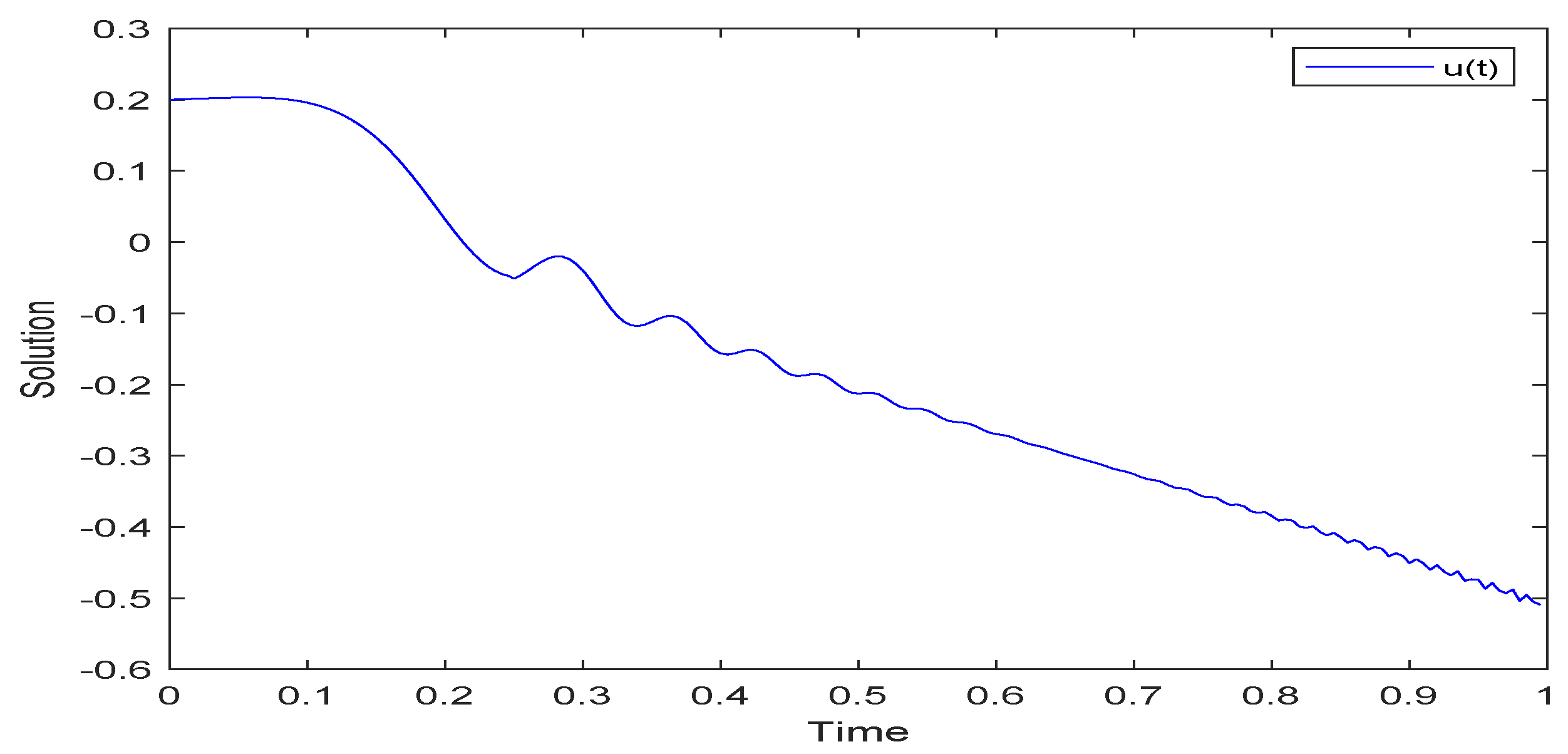
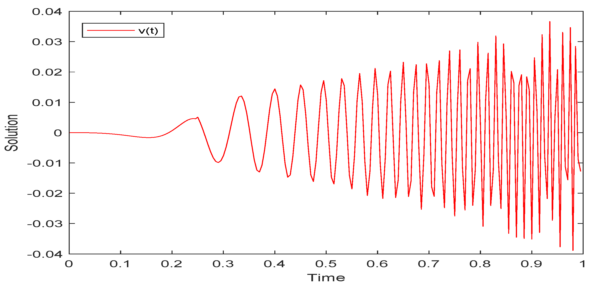
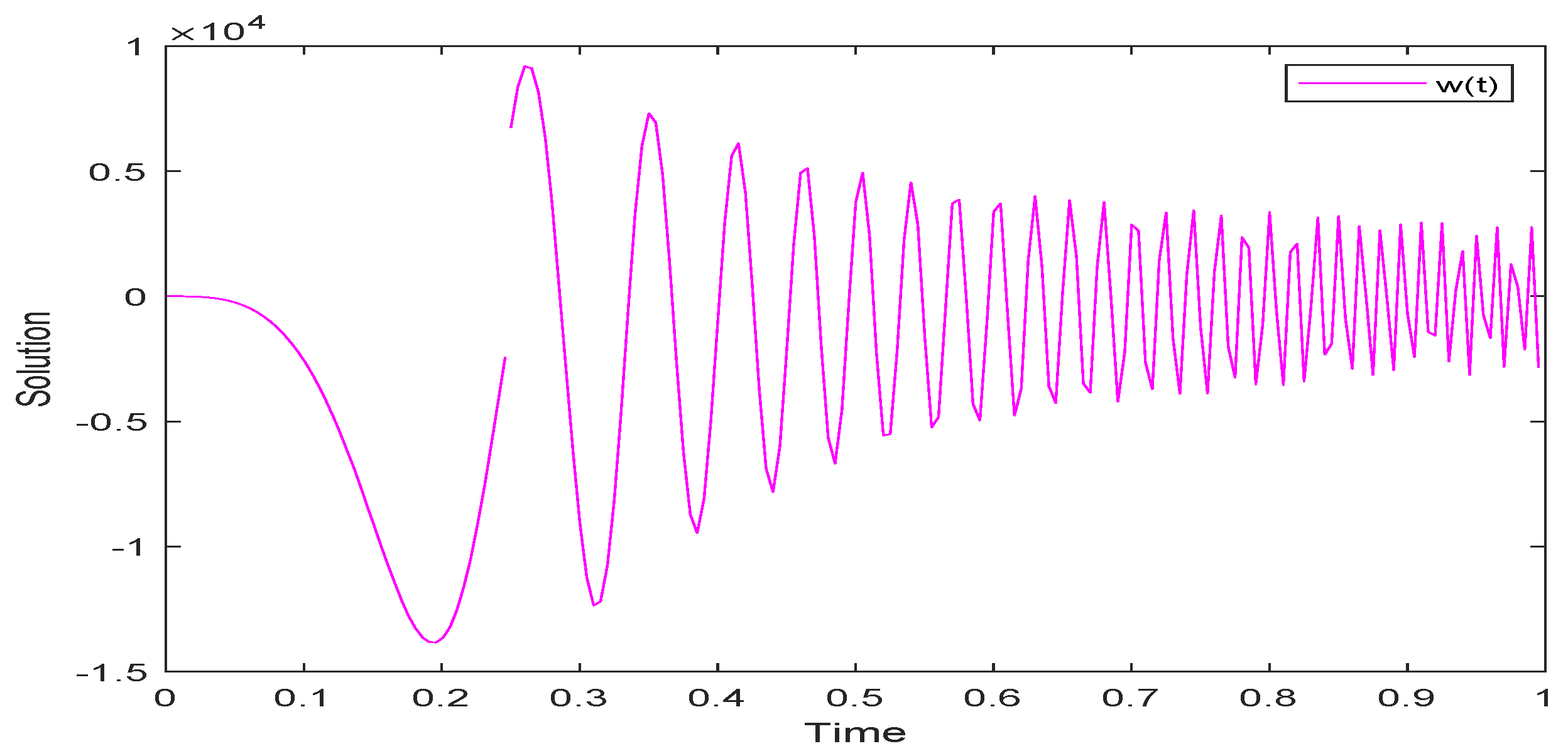
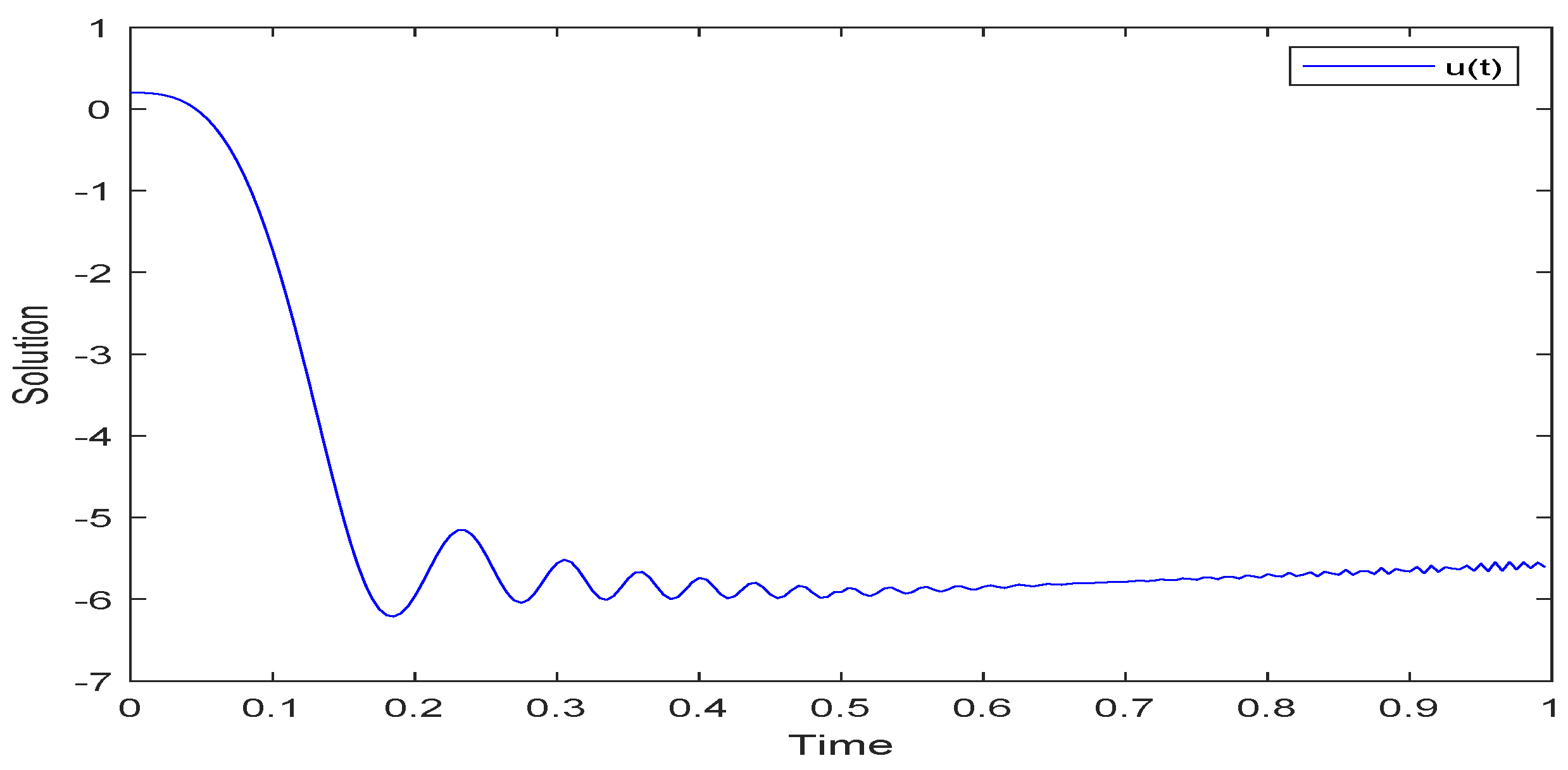
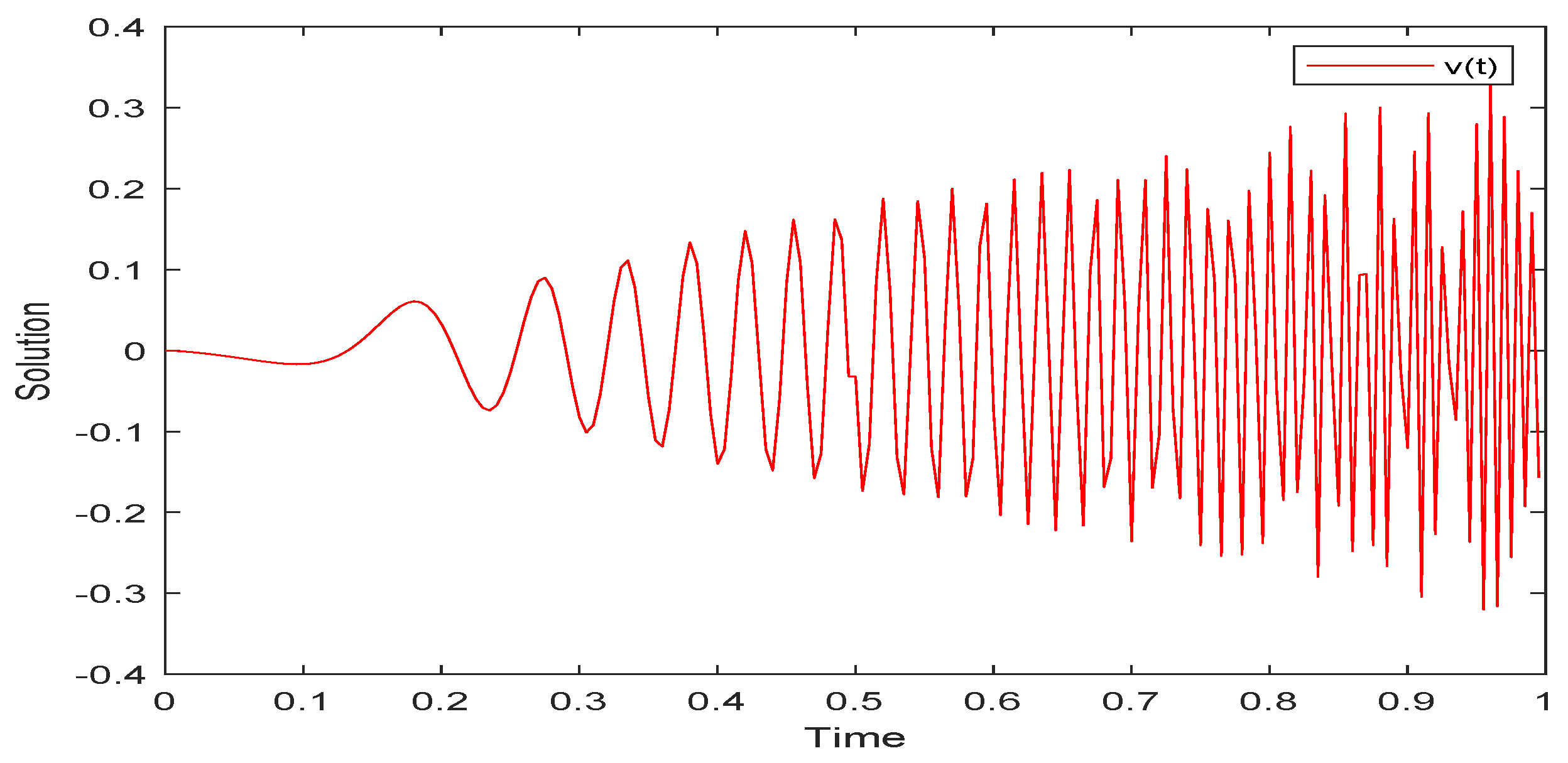
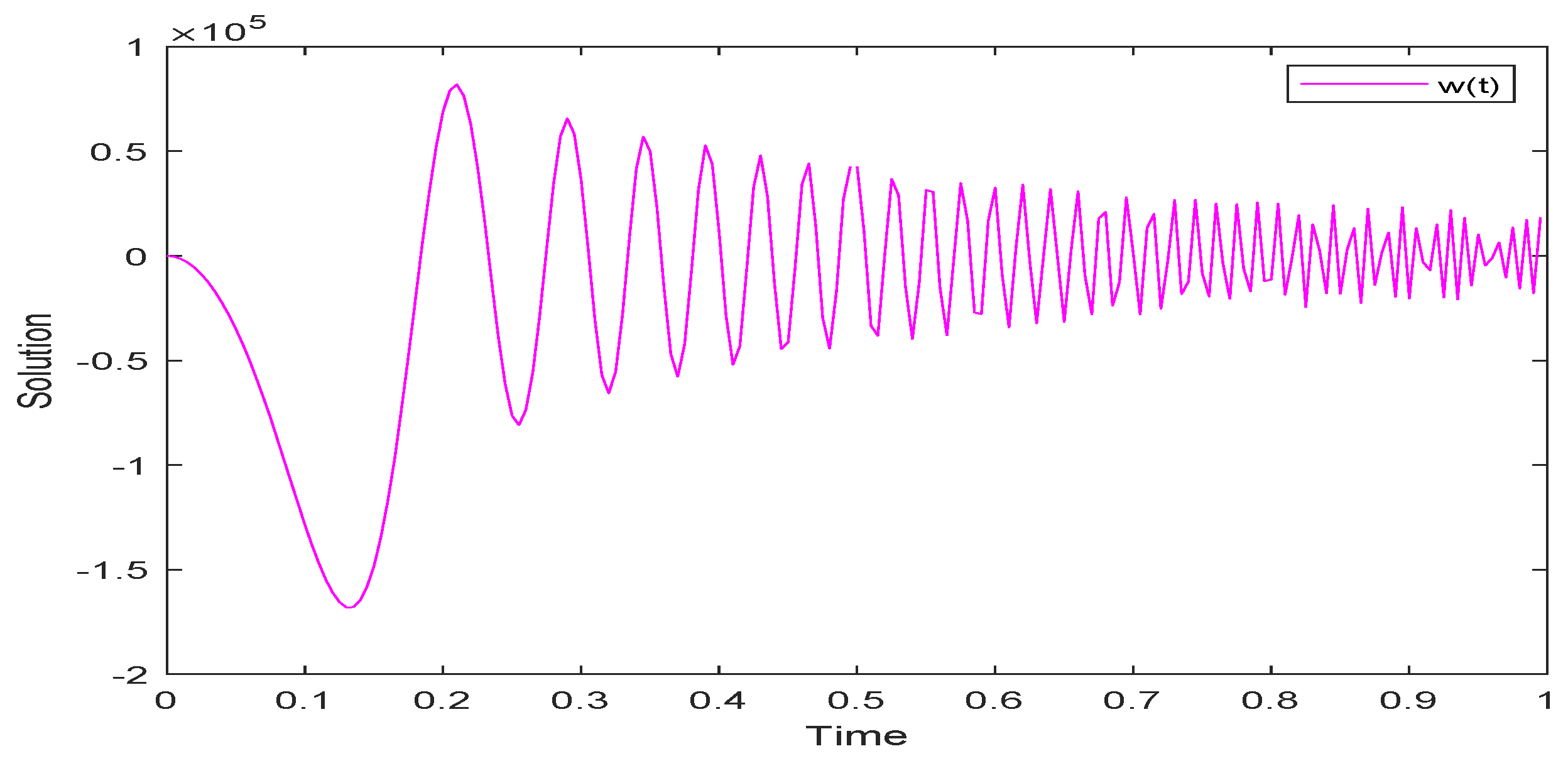
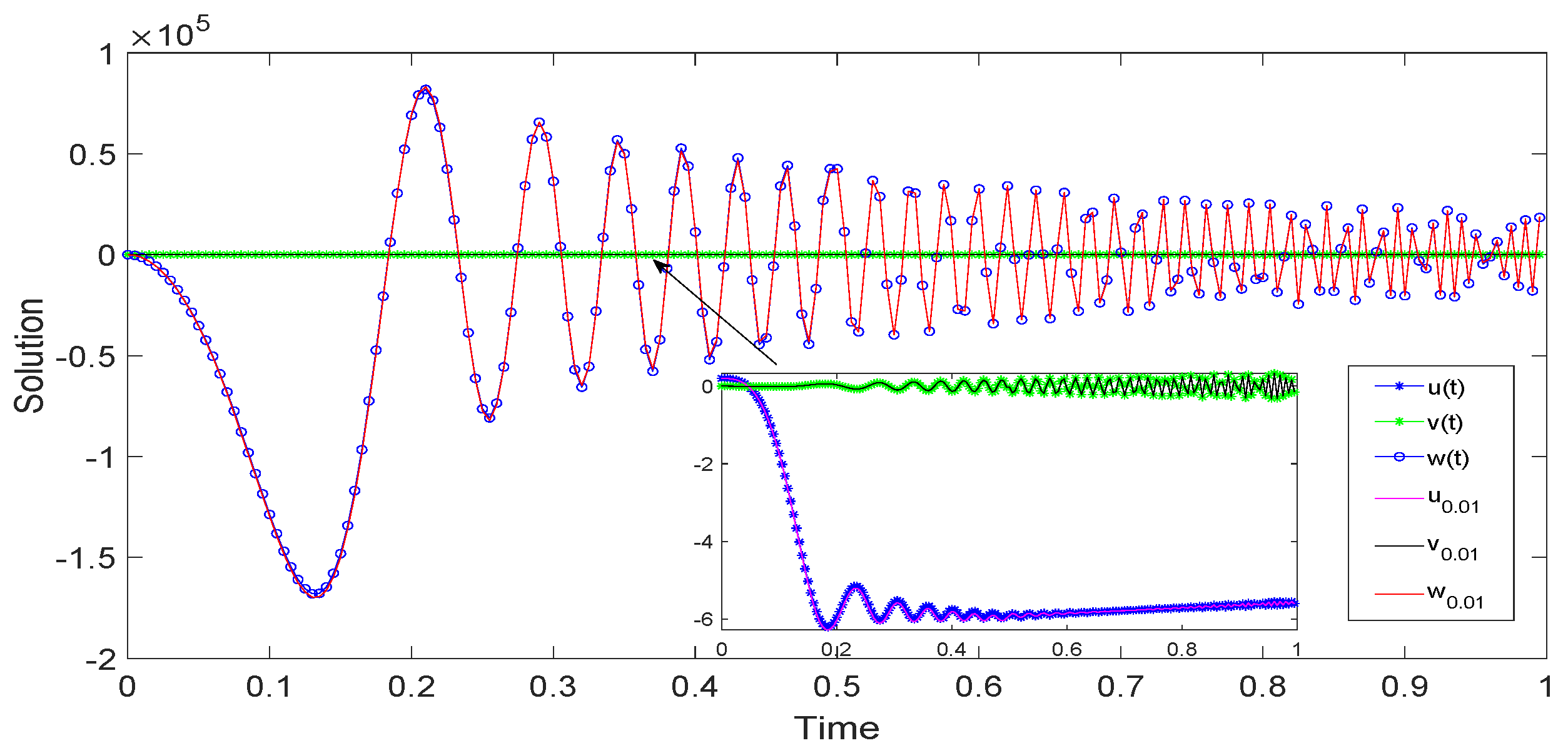
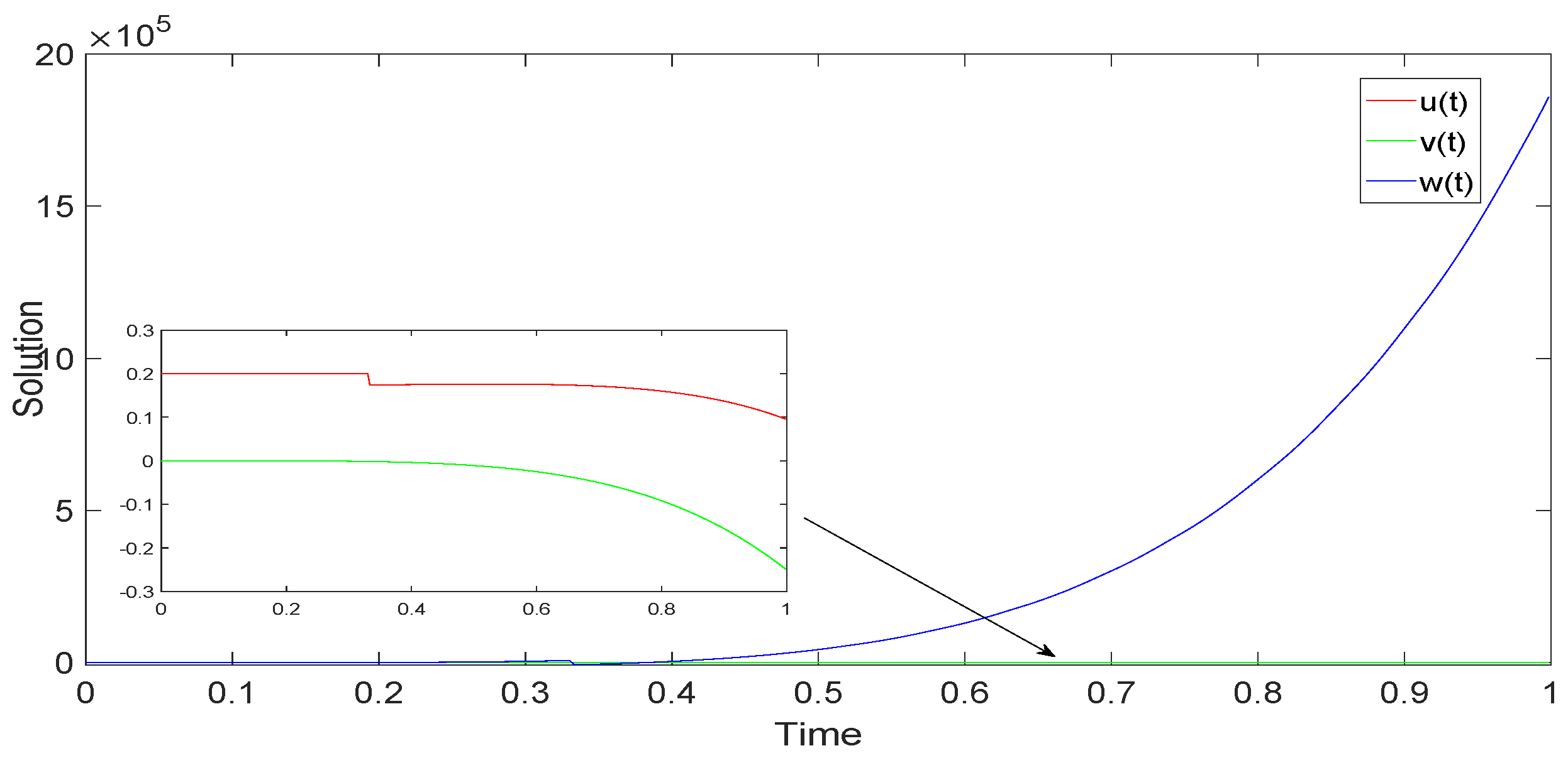
5. Examples and Simulations

Example 1.

Consider the following Riemann–Stieltjes IBVP:

$$\begin{array}{c}\hfill \left\{\begin{array}{c}{}^c\mathcal{D}_{0^{+}}^{2.9}u\left(t\right)+sin\left(\pi t\right)+{\displaystyle \frac{t}{30}}{u}_t+{\displaystyle \frac{t^2}{35}}{u}^{\prime }\left(t\right)+{\displaystyle \frac{t^3}{40}}{}^c\mathcal{D}_{0^{+}}^{{\displaystyle \frac{1}{2}}}u\left(t\right)=0,t\in [0,{\displaystyle \frac{1}{4}})\cup ({\displaystyle \frac{1}{4}},1],\hfill \\ {}^c\mathcal{D}_{0^{+}}^{{\displaystyle \frac{1}{2}}}u\left({{\displaystyle \frac{1}{4}}}^{+}\right)-{}^c\mathcal{D}_{0^{+}}^{{\displaystyle \frac{1}{2}}}u\left({{\displaystyle \frac{1}{4}}}^{-}\right)=I_1\left(u\left({\displaystyle \frac{1}{4}}\right)\right),\hfill \\ {\displaystyle \frac{1}{2}}u\left(0\right)-u^{\prime }\left(0\right)={\int }_0^1{h}_1(s,u\left(s\right))d{A}_1\left(s\right),\hfill \\ {\displaystyle \frac{1}{2}}u\left(1\right)+{\displaystyle \frac{2}{3}}{}^c\mathcal{D}_{0^{+}}^{{\displaystyle \frac{1}{3}}}u)\left(1\right)={\int }_0^1{h}_2(s,u\left(s\right))d{A}_2\left(s\right),\hfill \\ u^{\prime \prime }\left(0\right)=0,\hfill \\ u\left(s\right)=\varphi \left(s\right),s\in [-{\displaystyle \frac{1}{2}},0],\hfill \end{array}\right.\end{array}$$

(52)

where $q=2.9$, $p=\alpha =\gamma ={\displaystyle \frac{1}{2}}$, $\sigma ={\displaystyle \frac{1}{3}}$, $\beta =1$, $\delta ={\displaystyle \frac{2}{3}}$, $f(t,x,y,z)=sin\left(\pi t\right)+{\displaystyle \frac{tx}{30}}+{\displaystyle \frac{t^{2}y}{35}}+{\displaystyle \frac{t^{3}z}{40}}$, $h_1(s,u)={\displaystyle \frac{1}{3}}u$, $h_2(s,u)={\displaystyle \frac{1}{4}}u$, $A_1\left(s\right)=A_2\left(s\right)={\displaystyle \frac{1}{4}}s$, $I_1\left(u\right)={\displaystyle \frac{7}{10}}$, $\tau ={\displaystyle \frac{1}{2}}>0$, $\varphi \left(s\right)\in C_{{\displaystyle \frac{1}{2}}}$. By simple computation, we have ${\phi }_1={\displaystyle \frac{t}{30}}$, ${\phi }_2={\displaystyle \frac{t^2}{35}}$, ${\phi }_3={\displaystyle \frac{t^3}{40}}$, ${\varphi }_1={\displaystyle \frac{1}{3}}$, ${\varphi }_2={\displaystyle \frac{1}{4}}$, $L_1=0$, $\psi ={\displaystyle \frac{1}{30}}$,

$${\Delta }_1=\left|\begin{array}{cc}\alpha & -\beta \\ \gamma & \gamma +{\displaystyle \frac{\delta }{\Gamma (2-\sigma )}}\end{array}\right|=(\alpha +\beta )\gamma +{\displaystyle \frac{\alpha \delta }{\Gamma (2-\sigma )}}\approx 3.1284>0,$$

$$\tilde{M}={\displaystyle \frac{1}{\Gamma \left(q\right)}}+{\displaystyle \frac{\beta +\alpha }{{\Delta }_1-1}}\left[{\displaystyle \frac{\gamma }{\Gamma (q+1)}}+{\displaystyle \frac{\delta }{\Gamma (q-\sigma +1)}}\right]\approx 1.723,$$

$$\begin{array}{cc}\hfill {\kappa }_1=& {\displaystyle \frac{1}{{\Delta }_1}}(\gamma +{\displaystyle \frac{\delta }{\Gamma (2-\sigma )}}){\int }_0^1|{\varphi }_1\left(s\right)|d{A}_1\left(s\right)+{\displaystyle \frac{\beta +\alpha }{{\Delta }_1}}{\int }_0^1\left|{\varphi }_2\left(s\right)\right|d{A}_2\left(s\right)\hfill \\ & +\Gamma (2-p)\left[{\displaystyle \frac{\beta +\alpha }{{\Delta }_1}}(\gamma +{\displaystyle \frac{\delta }{\Gamma (2-\sigma )}})+1\right]t_1^{p-1}{L}_1\approx 0.0967,\hfill \end{array}$$

and

$${\vartheta }_1=3\psi \tilde{M}+{\kappa }_1\approx 0.269<1.$$

Thus, the conditions (H₁)–(H₄) are true. According to Theorem 1, we claim that system (52) has at least a solution on $I=[-{\displaystyle \frac{1}{2}},1]$.

Example 2.

Consider the Riemann–Stieltjes IBVP as follows:

$$\begin{array}{c}\hfill \left\{\begin{array}{c}{}^c\mathcal{D}_{0^{+}}^{{\displaystyle \frac{5}{2}}}u\left(t\right)+cos\left(\pi t\right)+{\displaystyle \frac{t}{30}}{u}_t+{\displaystyle \frac{t^2}{40}}{u}^{\prime }\left(t\right)+{\displaystyle \frac{t^3}{50}}{}^c\mathcal{D}_{0^{+}}^{{\displaystyle \frac{1}{2}}}u\left(t\right)=0,t\in [0,{\displaystyle \frac{1}{2}})\cup ({\displaystyle \frac{1}{2}},1],\hfill \\ {}^c\mathcal{D}_{0^{+}}^{{\displaystyle \frac{1}{2}}}u\left({{\displaystyle \frac{1}{2}}}^{+}\right)-{}^c\mathcal{D}_{0^{+}}^{{\displaystyle \frac{1}{2}}}u\left({{\displaystyle \frac{1}{2}}}^{-}\right)=I_1\left(u\left({\displaystyle \frac{1}{2}}\right)\right),\hfill \\ {\displaystyle \frac{1}{2}}u\left(0\right)-u^{\prime }\left(0\right)={\int }_0^1{h}_1(s,u\left(s\right))d{A}_1\left(s\right),\hfill \\ {\displaystyle \frac{1}{2}}u\left(1\right)+{\displaystyle \frac{4}{5}}({}^c\mathcal{D}_{0^{+}}^{{\displaystyle \frac{1}{2}}}u)\left(1\right)={\int }_0^1{h}_2(s,u\left(s\right))d{A}_2\left(s\right),\hfill \\ u^{\prime \prime }\left(0\right)=0,\hfill \\ u\left(s\right)=\varphi \left(s\right),s\in [-{\displaystyle \frac{1}{3}},0],\hfill \end{array}\right.\end{array}$$

(53)

where $q={\displaystyle \frac{5}{2}}$, $p=\alpha =\gamma =\sigma ={\displaystyle \frac{1}{2}}$, $\delta ={\displaystyle \frac{4}{5}}$, $\beta =1$, $f(t,x,y,z)=cos\left(\pi t\right)+{\displaystyle \frac{tx}{30}}+{\displaystyle \frac{t^{2}y}{40}}+{\displaystyle \frac{t^{3}z}{50}}$, $h_1(s,u)={\displaystyle \frac{1}{3}}u$, $h_2(s,u)={\displaystyle \frac{1}{4}}u$, $A_1\left(s\right)=A_2\left(s\right)={\displaystyle \frac{1}{4}}s$, $I_1\left(u\right)={\displaystyle \frac{9}{10}}$, $\tau ={\displaystyle \frac{1}{3}}>0$, $\varphi \left(s\right)\in C_{{\displaystyle \frac{1}{3}}}$. By simple computation, we have ${\phi }_1={\displaystyle \frac{t}{30}}$, ${\phi }_2={\displaystyle \frac{t^2}{40}}$, ${\phi }_3={\displaystyle \frac{t^3}{50}}$, ${\varphi }_1={\displaystyle \frac{1}{3}}$, ${\varphi }_2={\displaystyle \frac{1}{4}}$, $L_1=0$, $\psi ={\displaystyle \frac{1}{30}}$,

$${\Delta }_1=\left|\begin{array}{cc}\alpha & -\beta \\ \gamma & \gamma +{\displaystyle \frac{\delta }{\Gamma (2-\sigma )}}\end{array}\right|=(\alpha +\beta )\gamma +{\displaystyle \frac{\alpha \delta }{\Gamma (2-\sigma )}}\approx 1.2014>0,$$

$$\tilde{M}={\displaystyle \frac{1}{\Gamma \left(q\right)}}+{\displaystyle \frac{\beta +\alpha }{{\Delta }_1-1}}\left[{\displaystyle \frac{\gamma }{\Gamma (q+1)}}+{\displaystyle \frac{\delta }{\Gamma (q-\sigma +1)}}\right]\approx 4.8529,$$

$$\begin{array}{cc}\hfill {\kappa }_1=& {\displaystyle \frac{1}{{\Delta }_1}}(\gamma +{\displaystyle \frac{\delta }{\Gamma (2-\sigma )}}){\int }_0^1|{\varphi }_1\left(s\right)|d{A}_1\left(s\right)+{\displaystyle \frac{\beta +\alpha }{{\Delta }_1}}{\int }_0^1\left|{\varphi }_2\left(s\right)\right|d{A}_2\left(s\right)\hfill \\ & +\Gamma (2-p)\left[{\displaystyle \frac{\beta +\alpha }{{\Delta }_1}}(\gamma +{\displaystyle \frac{\delta }{\Gamma (2-\sigma )}})+1\right]t_1^{p-1}{L}_1\approx 0.1753,\hfill \end{array}$$

and

$${\vartheta }_1=3\psi \tilde{M}+{\kappa }_1\approx 0.6606<1.$$

So the conditions $\left({\mathrm{H}}_1\right)$-$\left({\mathrm{H}}_4\right)$ hold. One knows from Theorems 2 and 4 that IBVP (53) admits a UH-stable unique solution on $I=[-{\displaystyle \frac{1}{3}},1]$.

Example 3.

Consider the Riemann–Stieltjes IBVP for a delayed fractional differential equation with fractional-order impulses as follows:

$$\begin{array}{c}\hfill \left\{\begin{array}{c}{}^c\mathcal{D}_{0^{+}}^{{\displaystyle \frac{5}{2}}}u(t)+{\displaystyle \frac{t^3(u_t+u^{\prime }(t)+{}^c\mathcal{D}_{0^{+}}^{{\displaystyle \frac{1}{2}}}u(t){)}^2}{1+(u(t)+u^{\prime }(t)+{}^c\mathcal{D}_{0^{+}}^{{\displaystyle \frac{1}{2}}}u(t){)}^2}}=0,t\in [0,{\displaystyle \frac{1}{3}})\cup ({\displaystyle \frac{1}{3}},1],\hfill \\ {}^c\mathcal{D}_{0^{+}}^{{\displaystyle \frac{1}{2}}}u({{\displaystyle \frac{1}{3}}}^{+})-{}^c\mathcal{D}_{0^{+}}^{{\displaystyle \frac{1}{2}}}u({{\displaystyle \frac{1}{3}}}^{-})=I(u({\displaystyle \frac{1}{3}})),\hfill \\ {\displaystyle \frac{1}{2}}u(0)-u^{\prime }(0)={\int }_0^1{h}_1(s,u(s))d{A}_1(s),\hfill \\ {\displaystyle \frac{1}{2}}u(1)+{\displaystyle \frac{1}{2}}{(}^c{\mathcal{D}}_{0^{+}}^{{\displaystyle \frac{1}{2}}}u)(1)={\int }_0^1{h}_2(s,u(s))d{A}_2(s),\hfill \\ u^{\prime \prime }(0)=0,\hfill \\ u(s)=\varphi (s),s\in [-{\displaystyle \frac{1}{3}},0],\hfill \end{array}\right.\end{array}$$

(54)

where $q={\displaystyle \frac{5}{2}}$, $p=\alpha =\gamma =\delta =\sigma ={\displaystyle \frac{1}{2}}$, $\beta =1$, $f(t,x,y,z)={\displaystyle \frac{t^3{(x+y+z)}^2}{1+{(x+y+z)}^2}}$, $h_1(s,u)={\displaystyle \frac{1}{3}}su$, $h_2(s,u)={\displaystyle \frac{1}{4}}su$, $A_1\left(s\right)=A_2\left(s\right)={\displaystyle \frac{1}{4}}s$, $I_1\left(u\right)={\displaystyle \frac{1}{10}}u$, $\tau ={\displaystyle \frac{1}{3}}>0$, $\varphi \left(s\right)\in C_{{\displaystyle \frac{1}{3}}}$. Clearly, $\left|f(t,x,y,z)\right|⩽t^3=g\left(t\right)$, ${\rho }_1\left(s\right)={\displaystyle \frac{1}{3}}s$, ${\rho }_2\left(s\right)={\displaystyle \frac{1}{4}}s$, $H_1={\displaystyle \frac{1}{10}}$. By calculating, we obtain

$${\int }_0^1|{\rho }_1\left(s\right)|d{A}_1\left(s\right)={\displaystyle \frac{1}{24}},{\int }_0^1\left|{\rho }_2\left(s\right)\right|d{A}_2\left(s\right)={\displaystyle \frac{1}{32}},{\Delta }_1\approx 1.0321,$$

and

$$\begin{array}{cc}\hfill \zeta =& {\displaystyle \frac{1}{{\Delta }_1}}(\gamma +{\displaystyle \frac{\delta }{\Gamma (2-\sigma )}}){\int }_0^1|{\rho }_1\left(s\right)|d{A}_1\left(s\right)+{\displaystyle \frac{\alpha +\beta }{{\Delta }_1}}{\int }_0^1\left|{\rho }_2\left(s\right)\right|d{A}_2\left(s\right)\hfill \\ \hfill & +\Gamma (2-p)\left[{\displaystyle \frac{\alpha +\beta }{{\Delta }_1}}(\gamma +{\displaystyle \frac{\delta }{\Gamma (2-\sigma )}})+1\right]t_1^{p-1}{H}_1\approx 0.4793<1.\hfill \end{array}$$

Thus, all the conditions of Theorem 3 are satisfied. According to Theorem 3, we claim that system (54) has at least a solution on $I=[-{\displaystyle \frac{1}{3}},1]$.

To complete the numerical simulation of systems (52)–(54), a concise algorithm of (1) is outlined below:

Step 1: Let $v\left(t\right)=u^{\prime }\left(t\right)$ and $w\left(t\right))={}^c\mathcal{D}_{0^{+}}^{p}u\left(t\right)$, then (1) transforms into the impulsive integral nonlinear equations:

$$\begin{array}{c}\hfill \left\{\begin{array}{c}u\left(t\right)={\int }_0^{1}G(t,s)f(s,u_s,v\left(s\right),w\left(s\right))ds+{\displaystyle \frac{1}{{\Delta }_1}}[(1-t)\gamma +{\displaystyle \frac{\delta }{\Gamma (2-\sigma )}}]{\int }_0^1{h}_1(s,u\left(s\right))d{A}_1\left(s\right)\hfill \\ +{\displaystyle \frac{\beta +\alpha t}{{\Delta }_1}}{\int }_0^1{h}_2(s,u\left(s\right))d{A}_2\left(s\right)-{\displaystyle \frac{\Gamma (2-p)(\beta +\alpha t)}{{\Delta }_1}}[(\gamma +{\displaystyle \frac{\delta }{\Gamma (2-\sigma )}}){\displaystyle \sum _{j=1}^m}{t}_j^{p-1}{I}_j\left(u\left(t_j\right)\right)\hfill \\ -\gamma {\displaystyle \sum _{j=1}^m}{t}_j^p{I}_j\left(u\left(t_j\right)\right)]+\Gamma (2-p){\displaystyle \sum _{j=1}^l}{t}_j^{p-1}(t-t_j)I_j\left(u\left(t_j\right)\right),\hfill \\ v\left(t\right)={\int }_0^1{\displaystyle \frac{\partial G(t,s)}{\partial t}}f(s,u_s,v\left(s\right),w\left(s\right))ds-{\displaystyle \frac{\gamma }{{\Delta }_1}}{\int }_0^1{h}_1(s,u\left(s\right))d{A}_1\left(s\right)+{\displaystyle \frac{\alpha }{{\Delta }_1}}{\int }_0^1{h}_2(s,u\left(s\right))d{A}_2\left(s\right)\hfill \\ -{\displaystyle \frac{\Gamma (2-p)\alpha }{{\Delta }_1}}\left[(\gamma +{\displaystyle \frac{\delta }{\Gamma (2-\sigma )}}){\displaystyle \sum _{j=1}^m}{t}_j^{p-1}{I}_j\left(u\left(t_j\right)\right)-\gamma {\displaystyle \sum _{j=1}^m}{t}_j^p{I}_j\left(u\left(t_j\right)\right)\right]+\Gamma (2-p){\displaystyle \sum _{j=1}^l}{t}_j^{p-1}{I}_j\left(u\left(t_j\right)\right),\hfill \\ w\left(t\right)={\displaystyle \frac{1}{\Gamma (1-p)}}{\int }_0^t{(t-s)}^{-p}v\left(s\right)ds,t\in (t_l,t_{l+1}]\subset [0,1].\hfill \end{array}\right.\end{array}$$

(55)

Step 2: To take the derivative of system (55), one obtains the following nonlinear differential system (56). Next, numerical simulations can be conducted by applying ODE toolboxes in MATLAB.

$$\begin{array}{c}\hfill \left\{\begin{array}{c}{u}^{\prime }\left(t\right)=-{\displaystyle \frac{1}{\Gamma (q-1)}}{\int }_0^t{(t-s)}^{q-2}f(s,u_s,v\left(s\right),w\left(s\right))ds\hfill \\ +{\displaystyle \frac{\alpha }{{\Delta }_1}}{\int }_0^1\left[{\displaystyle \frac{\gamma }{\Gamma \left(q\right)}}{(1-s)}^{q-1}+{\displaystyle \frac{\delta }{\Gamma (q-\sigma )}}{(1-s)}^{q-\sigma -1}\right]f(s,u_s,v\left(s\right),w\left(s\right))ds\hfill \\ -{\displaystyle \frac{\gamma }{{\Delta }_1}}{\int }_0^1{h}_1(s,u\left(s\right))d{A}_1\left(s\right)+{\displaystyle \frac{\alpha }{{\Delta }_1}}{\int }_0^1{h}_2(s,u\left(s\right))d{A}_2\left(s\right)\hfill \\ -{\displaystyle \frac{\Gamma (2-p)\alpha }{{\Delta }_1}}\left[(\gamma +{\displaystyle \frac{\delta }{\Gamma (2-\sigma )}})\sum _{j=1}^m{t}_j^{p-1}{I}_j\left(u\left(t_j\right)\right)-\gamma \sum _{j=1}^m{t}_j^p{I}_j\left(u\left(t_j\right)\right)\right]\hfill \\ +\Gamma (2-p){\displaystyle \sum _{j=1}^l}{t}_j^{p-1}{I}_j\left(u\left(t_j\right)\right),\hfill \\ v^{\prime }\left(t\right)=-{\displaystyle \frac{1}{\Gamma (q-2)}}{\int }_0^t{(t-s)}^{q-3}f(s,u\left(s\right),v\left(s\right),w\left(s\right))ds,\hfill \\ w^{\prime }\left(t\right)=-{\displaystyle \frac{p}{\Gamma (1-p)}}{\int }_0^t{(t-s)}^{-p-1}v\left(s\right)ds,t\in (t_l,t_{l+1}]\subset [0,1].\hfill \end{array}\right.\end{array}$$

(56)

In line with the above algorithm, we have completed numerical simulations for three examples by ODE113 in MATLAB R2018b. The numerical simulation of system (52) is shown as Figure 1, Figure 2 and Figure 3. The numerical simulation and UH stability of system (53) are shown as Figure 4, Figure 5, Figure 6 and Figure 7. The numerical simulation of system (54) is shown as Figure 8. From Figure 1, Figure 2, Figure 3, Figure 4, Figure 5 and Figure 6, it can be seen that the solutions of systems (53) and (54) are oscillatory because the systems contain periodic terms $sin\left(\pi t\right)$ and $cos\left(\pi t\right)$. However, the solutions of system (52) do not oscillate.

6. Conclusions

In the manuscript, a delayed fractional system (1) and (2) with fractional-order impulses is studied. Compared with some previous studies, our system is a more complex functional differential equation that combines delay effects, fractional-order impulses, and Riemann–Stieltjes IBVPs. The system optimizes the nonlinear fractional differential system in reference [9]. By using differential inequality techniques and some fixed-point theorems, the existence and uniqueness of solutions are obtained. Meanwhile, we apply mathematical analysis to discuss the UH-stability of the system. Finally, we provide an algorithm and conduct numerical simulations on three examples to demonstrate the correctness and availability of our main results. In addition, there are two topics that need further study in the future. One is the general higher-order delayed fractional differential equation with different types of boundary value conditions and impulses. The other is the delayed coupled fractional differential system with different types of boundary value conditions and impulses.

References

1. Atangana, A.; Alkahtani, B. Extension of the resistance, inductance, capacitance electrical circuit to fractional derivative without singular kernel. Adv. Mech. Eng. 2015, 7, 1–6. [Google Scholar] [CrossRef]
2. Alizadeh, S.; Baleanu, D.; Rezapour, S. Analyzing transient response of the parallel RCL circuit by using the Caputo-Fabrizio fractional derivative. Adv. Differ. Equ. 2020, 2020, 55. [Google Scholar] [CrossRef]
3. Baleanu, D.; Jajarmi, A.; Mohammadi, H.; Rezapour, S. A new study on the mathematical modelling of human liver with Caputo-Fabrizio fractional derivative. Chaos Soliton. Fract. 2020, 134, 109705. [Google Scholar] [CrossRef]
4. Rahman, M.; Ahmad, S.; Matoog, R.; Alshehri, N.; Khan, T. Study on the mathematical modelling of COVID-19 with Caputo-Fabrizio operator. Chaos Soliton. Fract. 2021, 150, 111121. [Google Scholar] [CrossRef] [PubMed]
5. Javidi, M.; Ahmad, B. Dynamic analysis of time fractional order phytoplankton-toxic phytoplankton-zooplankton system. Ecol. Model. 2015, 318, 8–18. [Google Scholar] [CrossRef]
6. Chatterjee, A.; Ahmad, B. A fractional-order differential equation model of COVID-19 infection of epithelial cells. Chaos Soliton. Fract. 2021, 147, 110952. [Google Scholar] [CrossRef]
7. Zhao, K. Stability of a nonlinear ML-nonsingular kernel fractional Langevin system with distributed lags and integral control. Axioms 2022, 11, 350. [Google Scholar] [CrossRef]
8. Zhao, K. Stability of a nonlinear Langevin system of ML-type fractional derivative affected by time-varying delays and differential feedback control. Fractal Fract. 2022, 6, 725. [Google Scholar] [CrossRef]
9. Li, M.; Sun, J.; Zhao, Y. Existence of positive solution for BVP of nonlinear fractional differential equation with integral boundary conditions. Adv. Differ. Equ. 2020, 2020, 177. [Google Scholar] [CrossRef]
10. Zhang, X.; Liu, L.; Wu, Y. Multiple positive solutions of a singular fractional differential equation with negatively perturbed term. Math. Comput. Model. 2012, 55, 1263–1274. [Google Scholar] [CrossRef]
11. Zhao, Y.; Sun, S.; Han, Z.; Zhang, M. Positive solutions for boundary value problems of nonlinear fractional differential equations. Appl. Math. Comput. 2011, 217, 6950–6958. [Google Scholar]
12. Zhang, S. Positive solutions to singular boundary value problem for nonlinear fractional differential equation. Comput. Math. Appl. 2010, 59, 1300–1309. [Google Scholar] [CrossRef]
13. Wang, Y.; Liu, L.; Wu, Y. Positive solutions for a class of fractional boundary value problem with changing sign nonlinearity. Nonlinear Anal.-Theor. 2011, 74, 6434–6441. [Google Scholar] [CrossRef]
14. Liu, Y. Solvability of anti-periodic BVPs for impulsive fractional differential systems involving Caputo and Riemann-Liouville fractional derivatives. Int. J. Nonlinear Sci. Numer. Simul. 2018, 19, 125–152. [Google Scholar] [CrossRef]
15. Jiang, D.; Yuan, C. The positive properties of the green function for Dirichlet-type boundary value problems of nonlinear fractional differential equations and its application. Nonlinear Anal. TMA 2010, 72, 710–719. [Google Scholar] [CrossRef]
16. Wang, Y.; Liu, L. Positive properties of the green function for two-term fractional differential equations and its application. J. Nonlinear Sci. Appl. 2017, 10, 2094–2102. [Google Scholar] [CrossRef]
17. Cao, J.; Chen, H. Impulsive fractional differential equations with nonlinear boundary conditions. Math. Comput. Model. 2012, 55, 303–311. [Google Scholar] [CrossRef]
18. Bai, C. Impulsive periodic boundary value problems for fractional differential equation involving Riemann-Liouville sequential fractional derivative. J. Math. Anal. Appl. 2011, 384, 211–231. [Google Scholar] [CrossRef]
19. Wang, G.; Ahmad, B.; Zhang, L. Impulsive anti-periodic boundary value problem for nonlinear differential equations of fractional order. Nonlinear Anal.-Theor. 2011, 74, 792–804. [Google Scholar] [CrossRef]
20. Zhao, K. Existence and UH-stability of integral boundary problem for a class of nonlinear higher-order Hadamard fractional Langevin equation via Mittag-Leffler functions. Filomat 2023, 37, 1053–1063. [Google Scholar] [CrossRef]
21. Ahmad, B.; Alghanmi, M.; Ntouyas, S.; Alsaedi, A. Fractional differential equations involving generalized derivative with Stieltjes and fractional integral boundary conditions. Appl. Math. Lett. 2018, 84, 111–117. [Google Scholar] [CrossRef]
22. Ulam, S. A Collection of Mathematical Problems. Interscience Tracts in Pure and Applied Mathmatics; Interscience: New York, NY, USA, 1906. [Google Scholar]
23. Hyers, D. On the stability of the linear functional equation. Proc. Natl. Acad. Sci. USA 1941, 27, 2222–2240. [Google Scholar] [CrossRef] [PubMed]
24. Forti, G. Hyers-Ulam stability of functional equations in several variables. Aeq. Math. 1995, 50, 143–190. [Google Scholar] [CrossRef]
25. Brzdek, J.; Popa, D.; Raşa, I.; Xu, B. Ulam Stability of Operators; Academic Press: London, UK, 2018. [Google Scholar]
26. Hyers, D.; Isac, G.; Rassias, T. Stability of Functional Equations in Several Variables; Birkhäuser: Boston, MA, USA, 1998. [Google Scholar]
27. Czerwik, S. Functional Equations and Inequalities in Several Variables; World Scientific: Singapore, 2002. [Google Scholar]
28. Aderyani, S.; Saadati, R.; Li, C.; Allahviranloo, T. Towards Ulam Type Multi Stability Analysis; Springer: Cham, Switzerland, 2024. [Google Scholar]
29. Zhao, K. Solvability, Approximation and Stability of Periodic Boundary Value Problem for a Nonlinear Hadamard Fractional Differential Equation with p-Laplacian. Axioms 2023, 12, 733. [Google Scholar] [CrossRef]
30. Zhao, K.; Liu, J.; Lv, X. A Unified Approach to Solvability and Stability of Multipoint BVPs for Langevin and Sturm-Liouville Equations with CH-Fractional Derivatives and Impulses via Coincidence Theory. Fractal Fract. 2024, 8, 111. [Google Scholar] [CrossRef]
31. Rezaei, H.; Jung, S.; Rassias, T. Laplace transform and Hyers-Ulam stability of linear differential equations. J. Math. Anal. Appl. 2013, 403, 244–251. [Google Scholar] [CrossRef]
32. Lv, X.; Zhao, K.; Xie, H. Stability and Numerical Simulation of a Nonlinear Hadamard Fractional Coupling Laplacian System with Symmetric Periodic Boundary Conditions. Symmetry 2024, 16, 774. [Google Scholar] [CrossRef]
33. Zhao, K. Study on the stability and its simulation algorithm of a nonlinear impulsive ABC-fractional coupled system with a Laplacian operator via F-contractive mapping. Adv. Contin. Discret. Model. 2024, 2024, 5. [Google Scholar] [CrossRef]
34. Wang, C.; Xu, T. Hyers-Ulam stability of fractional linear differential equations involving Caputo fractional derivatives. Appl. Math. Comput. 2015, 60, 383–393. [Google Scholar] [CrossRef]
35. Wang, J.; Li, X. Ulam-Hyers stability of fractional Langevin equations. Appl. Math. Comput. 2015, 258, 72–83. [Google Scholar] [CrossRef]
36. Zhao, K. Existence, stability and simulation of a class of nonlinear fractional Langevin equations involving nonsingular Mittag-Leffler kernel. Fractal Fract. 2022, 6, 469. [Google Scholar] [CrossRef]
37. Podlubny, I. Fractional Differential Equations; Academic Press: New York, NY, USA, 1993. [Google Scholar]
38. Klbas, A.; Srivastava, H.; Trujillo, J. Theory and Applications of Fractional Differential Equation; Elsevier: Amsterdam, The Netherlands, 2006. [Google Scholar]
39. Guo, D.; Lakshmikantham, V. Nonlinear Problems in Abstract Cone; Academic Press: Orlando, FL, USA, 1988. [Google Scholar]
Figure 1. Simulation of solution u ( t ) for system (52).
Axioms 13 00682 g001
Figure 2. Simulation of solution v ( t ) for system (52).
Axioms 13 00682 g002
Figure 3. Simulation of solution w ( t ) for system (52).
Axioms 13 00682 g003
Figure 4. Simulation of solution u ( t ) for system (53).
Axioms 13 00682 g004
Figure 5. Simulation of solution v ( t ) for system (53).
Axioms 13 00682 g005
Figure 6. Simulation of solution w ( t ) for system (53).
Axioms 13 00682 g006
Figure 7. Evolution of UH-stability with ϵ = 0.01 for system (53).
Axioms 13 00682 g007
Figure 8. Evolution of dynamic behaviors for system (54).
Axioms 13 00682 g008
Disclaimer/Publisher’s Note: The statements, opinions and data contained in all publications are solely those of the individual author(s) and contributor(s) and not of MDPI and/or the editor(s). MDPI and/or the editor(s) disclaim responsibility for any injury to people or property resulting from any ideas, methods, instructions or products referred to in the content.