


An Analysis of Type-I Generalized Progressive Hybrid Censoring for the One Parameter Logistic-Geometry Lifetime Distribution with Applications


Abstract
1. Introduction
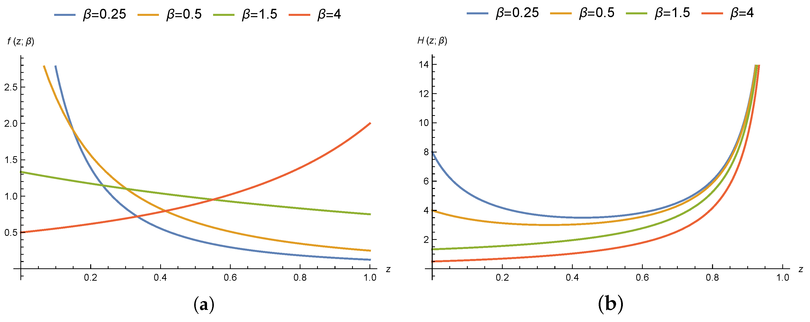
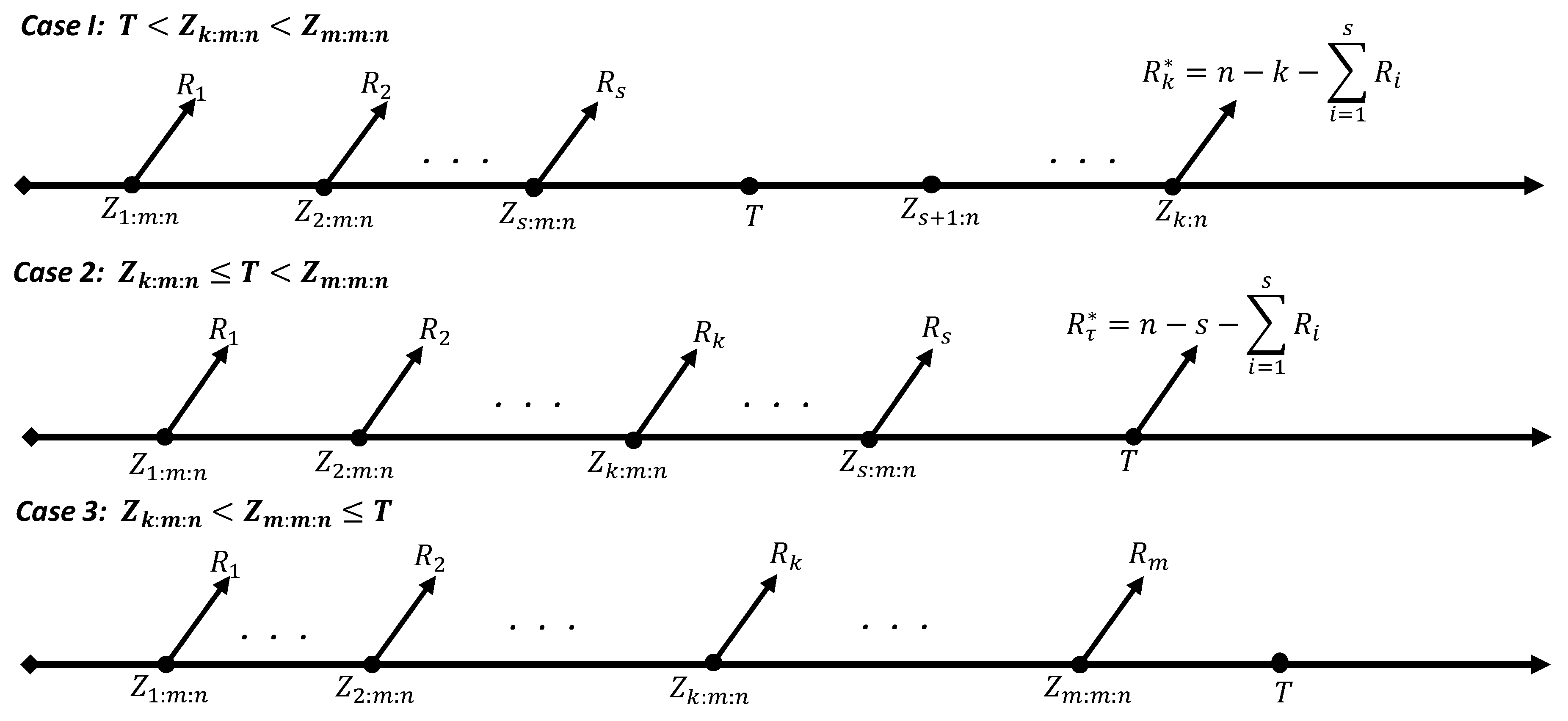
2. The Model Clarification
3. Maximum Likelihood Evaluation
- After setting , estimate the parameter using the moments technique or another way to serve as the starting value for iterations; the estimates are then denoted as ().
- Now, we can determine , along with the Fisher information matrix that was seen .
- Update as
- After setting , return to Step 1.
- Iterate repeatedly until is less than a predetermined threshold. The MLE of the parameters, represented as , represents the final estimations of .
Asymptotic Confidence Intervals
4. Bootstrap Interval Estimation
4.1. Bootstrap-p Interval Estimation
- Based on the original data , obtain by maximizing Equation (10).
- Based on the generalized progressive censoring scheme generate a type-II progressive censoring sample from the parameterized UHLG distribution , applying the method outlined in [19].
- Obtain the MLEs from the bootstrap sample and use to denote the bootstrap estimate. In this case, might be , , and .
- To obtain the intended results, steps (2) and (3) need be carried out N boot times.
- Arrange in ascending order.
4.2. Bootstrap-t Interval Estimation
- Equation (10) may be maximized to produce based on the original data.
- Based on the generalized progressive censoring scheme , generate a Type-II progressive censoring sample from the adjustable UHLG distribution , following the method stated in [19].
- A bootstrap estimate is indicated by (in our example, might) be , , and . Obtain the MLEs based on the bootstrap sample.
- Equation (10) may be maximized to produce based on the original data.
- The value of the statistic can be defined as
- Steps 2 through 5 should be repeated N times to obtain .
- Sort in ascending order to produce the sequences that are ordered. .
5. Bayes Estimation
| Algorithm 1: MCMC method |
|
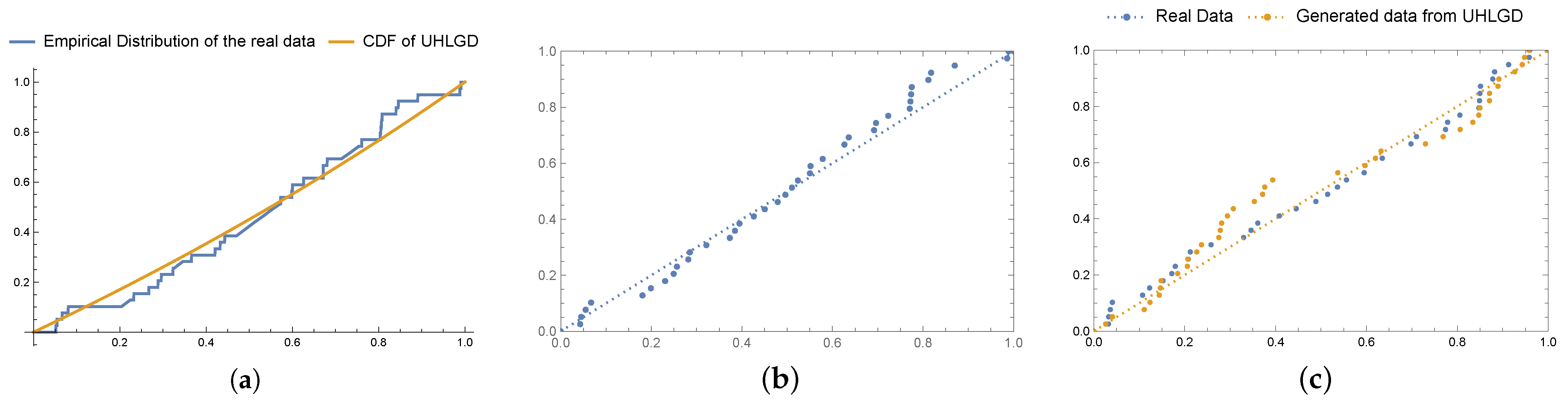
6. Real Data Application
7. Simulation Study
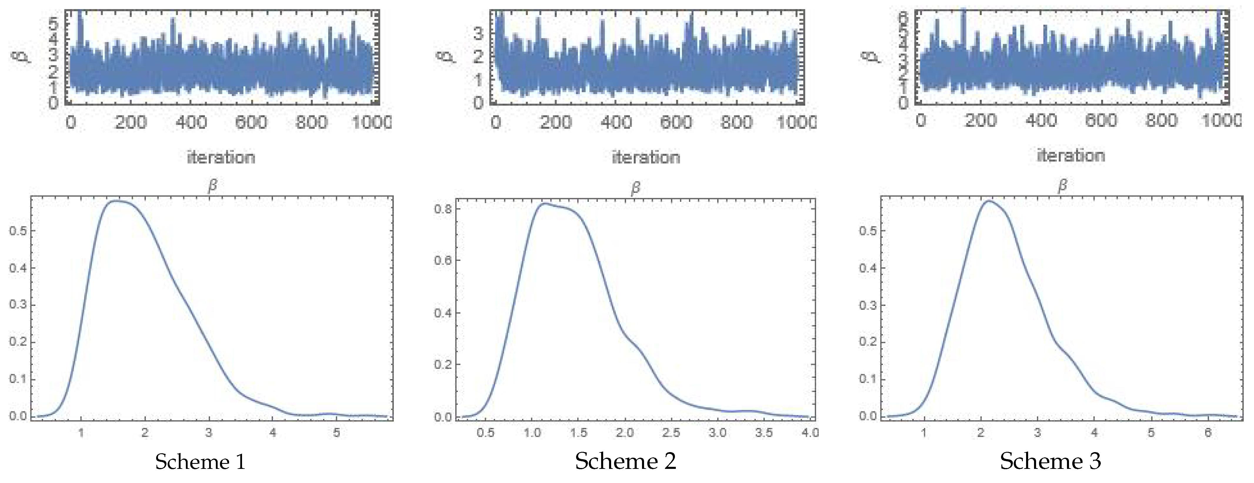
- Scheme 1: .
- Scheme 2: .
- Scheme 3: .
8. Conclusions and Discussion
- The MLEs and the Bayesian estimates based on the non-informative priors function semi-equally in most circumstances, as the MSE shows.
- We observed that the GEL outperforms the SEL and LINEX loss functions in the Bayesian estimation.
- Generally speaking, the MSE falls as n and m rise.
- As T increases, the average length of the confidence intervals decreases.
- The bootstrap-p confidence intervals have the highest coverage probability in a large proportion of situations.
- Compared to Schemes 2 and 3, censoring Scheme 1 performs better.
- We have observed that the projections are rather close to those of the entire sample because of the real data estimates.
Author Contributions
Funding
Data Availability Statement
Acknowledgments
Conflicts of Interest
References
- Epstein, B. Truncated life tests in the exponential case. Ann. Math. Stat. 1954, 25, 555–564. [Google Scholar] [CrossRef]
- Childs, A.; Chandrasekar, B.; Balakrishnan, N.; Kundu, D. Exact likelihood inference based on Type-I and Type-II hybrid censored samples from the exponential distribution. Ann. Inst. Stat. Math. 2003, 55, 319–330. [Google Scholar] [CrossRef]
- Balakrishnan, N.; Balakrishnan, N.; Aggarwala, R. Progressive Censoring: Theory, Methods, and Applications; Birkhäuser: Boston, UK, 2000. [Google Scholar]
- Cho, Y.; Sun, H.; Lee, K. Exact likelihood inference for an exponential parameter under generalized progressive hybrid censoring scheme. Stat. Methodol. 2015, 23, 18–34. [Google Scholar] [CrossRef]
- Lee, K.; Sun, H.; Cho, Y. Exact likelihood inference of the exponential parameter under generalized Type II progressive hybrid censoring. J. Korean Stat. Soc. 2016, 45, 123–136. [Google Scholar] [CrossRef]
- Nagy, M.; Sultan, K.S.; Abu-Moussa, M.H. Analysis of the generalized progressive hybrid censoring from Burr Type-XII lifetime model. AIMS Math. 2021, 6, 9675–9704. [Google Scholar] [CrossRef]
- Nagy, M.; Bakr, M.E.; Alrasheedi, A.F. Analysis with Applications of the Generalized Type-II Progressive Hybrid Censoring Sample from Burr Type-XII Model. Math. Probl. Eng. 2022, 2022, 1241303. [Google Scholar] [CrossRef]
- Nagy, M.; Alrasheedi, A.F. The lifetime analysis of the Weibull model based on Generalized Type-I progressive hybrid censoring schemes. Math. Biosci. Eng. 2022, 19, 2330–2354. [Google Scholar] [CrossRef]
- Nagy, M.; Alrasheedi, A.F. Estimations of generalized exponential distribution parameters based on type I generalized progressive hybrid censored data. Comput. Math. Methods Med. 2022, 2022, 8058473. [Google Scholar] [CrossRef]
- Varian, H.R. A Bayesian approach to real estate assessment. Stud. Bayesian Econom. Stat. Honor. Leonard J. Savage 1975, 195–208. [Google Scholar]
- Nagy, M.; Abu-Moussa, M.H.; Alrasheedi, A.F.; Rabie, A. Expected Bayesian estimation for exponential model based on simple step stress with Type-I hybrid censored data. Math. Biosci. Eng. 2022, 19, 9773–9791. [Google Scholar] [CrossRef]
- Ramadan, A.T.; Tolba, A.H.; El-Desouky, B.S. A unit half-logistic geometric distribution and its application in insurance. Axioms 2022, 11, 676. [Google Scholar] [CrossRef]
- Ahmed, E.A. Estimation of some lifetime parameters of generalized Gompertz distribution under progressively type-II censored data. Appl. Math. Model. 2015, 39, 5567–5578. [Google Scholar] [CrossRef]
- Mahmoud, M.A.W.; Ramadan, D.A.; Mansour, M.M.M. Estimation of lifetime parameters of the modified extended exponential distribution with application to a mechanical model. Commun. Stat. Simul. Comput. 2022, 51, 7005–7018. [Google Scholar] [CrossRef]
- Tolba, A. Bayesian and non-Bayesian estimation methods for simulating the parameter of the Akshaya distribution. Comput. J. Math. Stat. Sci. 2022, 1, 13–25. [Google Scholar] [CrossRef]
- Greene, W.H. Econometric Analysis, 4th ed.; International edition; Prentice Hall: Hoboken, NJ, USA, 2000; pp. 201–215. [Google Scholar]
- Efron, B. The Jackknife, The Bootstrap and Other Resampling Plans; Society for Industrial and Applied Mathematics: Philadelphia, PA, USA, 1982. [Google Scholar]
- Hall, P. Theoretical comparison of bootstrap confidence intervals. Ann. Stat. 1988, 16, 927–953. [Google Scholar] [CrossRef]
- Balakrishnan, N.; Sandhu, R.A. Best linear unbiased and maximum likelihood estimation for exponential distributions under general progressive type-II censored samples. Sankhyā Indian J. Stat. Ser. 1996, 58, 1–9. [Google Scholar]
- Dutta, S.; Ng, H.K.T.; Kayal, S. Inference for a general family of inverted exponentiated distributions under unified hybrid censoring with partially observed competing risks data. J. Comput. Appl. Math. 2023, 422, 114934. [Google Scholar] [CrossRef]
- Smith, A.F.; Roberts, G.O. Bayesian computation via the Gibbs sampler and related Markov chain Monte Carlo methods. J. R. Stat. Soc. Ser. B 1993, 55, 3–23. [Google Scholar] [CrossRef]
- Ahmed, E.A. Estimation and prediction for the generalized inverted exponential distribution based on progressively first-failure-censored data with application. J. Appl. Stat. 2017, 44, 1576–1608. [Google Scholar] [CrossRef]
- Panahi, H.; Asadi, S. On adaptive progressive hybrid censored Burr type III distribution: Application to the nano droplet dispersion data. Qual. Technol. Quant. Manag. 2021, 18, 179–201. [Google Scholar] [CrossRef]
- Abushal, T.A. Parametric inference of Akash distribution for Type-II censoring with analyzing of relief times of patients. Aims Math. 2021, 6, 10789–10801. [Google Scholar] [CrossRef]
- Xu, A.; Fang, G.; Zhuang, L.; Gu, C. A multivariate student-t process model for dependent tail-weighted degradation data. IISE Trans. 2024, 1–23. [Google Scholar] [CrossRef]
- Abd El-Raheem, A.E.; Hosny, M.; Abu-Moussa, M.H. On progressive censored competing risks data: Real data application and simulation study. Mathematics 2021, 9, 1805. [Google Scholar] [CrossRef]
- Hoel, D.G. A representation of mortality data by competing risks. Biometrics 1972, 28, 475–488. [Google Scholar] [CrossRef]

| 0.0519 | 0.0545 | 0.0662 | 0.0805 | 0.2117 | 0.2325 | 0.2675 | 0.2883 | 0.2961 |
| 0.3234 | 0.3273 | 0.3662 | 0.4207 | 0.4325 | 0.4428 | 0.4753 | 0.5000 | 0.5286 |
| 0.5454 | 0.5597 | 0.5727 | 0.5987 | 0.6000 | 0.6259 | 0.6714 | 0.6714 | 0.6805 |
| 0.7325 | 0.7364 | 0.7610 | 0.8038 | 0.8052 | 0.8065 | 0.8078 | 0.8403 | 0.8454 |
| 0.8909 | 0.9883 | 0.9909 |
| Statistic | p-Value | |
|---|---|---|
| Kolmogorov–Smirnov | 0.1053 | 0.7406 |
| Anderson–Darling | 0.5028 | 0.7426 |
| Cramér-von Mises | 0.0675 | 0.7668 |
| Pearson | 6.9231 | 0.5449 |
| Scheme | T | R and Sample |
|---|---|---|
| Sch. 1 | 0.3 | (1, 0, 0, 1, 0, 1, 0, 1, 0, 0, 0, 0, 0, 0, 0, 0, 0, 17), |
| x = (0.0519, 0.0545, 0.0662, 0.0805, 0.2324, 0.2675, 0.2883 | ||
| 0.2961, 0.3234, 0.3273, 0.3662, 0.4207, 0.4325, 0.4428 | ||
| 0.4753, 0.5000, 0.5286, 0.54545) | ||
| Sch. 2 | 0.7 | R = (1, 0, 0, 1, 0, 1, 0, 1, 0, 1, 0, 1, 0, 1, 0, 1, 0, 1, 0, 1, 0, 1), |
| x = (0.05194, 0.0545, 0.0662, 0.0805, 0.2324, 0.2675, 0.2883 | ||
| 0.2961, 0.3234, 0.3273, 0.3662, 0.4208, 0.4325, 0.4428 | ||
| 0.4753, 0.5000, 0.5286, 0.5454, 0.5597, 0.6000, 0.6714) | ||
| Sch. 3 | 0.9 | R = (1, 0, 0, 1, 0, 1, 0, 1, 0, 1, 0, 1, 0, 1, 0, 1, 0, 1, 0, 1, 0, |
| 1, 0, 1, 2), | ||
| (0.05194, 0.05454, 0.06623, 0.08052, 0.23247, 0.26753, 0.28831 | ||
| 0.2961, 0.3234, 0.3273, 0.3662, 0.4207, 0.4325, 0.4428 | ||
| 0.4753, 0.5000, 0.5286, 0.5454, 0.5597, 0.5727, 0.6000, | ||
| 0.6714, 0.7325, 0.7364, 0.7610) |
| Parameter | Scheme | MLE (Complete) | MLE | BNIFS | BNIFL | BNIFG |
|---|---|---|---|---|---|---|
| Sch. 1 | 2.6948 | 2.8581 | 2.6806 | 2.6640 | ||
| Sch. 2 | 2.4775 | 2.6045 | 2.4678 | 2.4424 | ||
| Sch. 3 | 2.3639 | 2.4737 | 2.3559 | 2.3273 | ||
| Sch. 1 | 0.4732 | 0.4766 | 0.4752 | 0.4677 | ||
| Sch. 2 | 0.4523 | 0.4550 | 0.4537 | 0.4464 | ||
| Sch. 3 | 0.4407 | 0.4430 | 0.4418 | 0.4347 | ||
| Sch. 1 | 2.1950 | 2.1807 | 2.1564 | 2.1459 | ||
| Sch. 2 | 2.2821 | 2.2710 | 2.2490 | 2.2408 | ||
| Sch. 3 | 2.3304 | 2.3210 | 2.3002 | 2.2932 |
| Parameter | Scheme | (L, U) | AL | (L, U) | AL | (L, U) | AL | (L, U) | AL |
| Sch. 1 | (1.098, 4.292) | 3.194 | (1.713, 4.422) | 2.710 | (0.988, 3.585) | 2.597 | (0.000, 3.367) | 5.316 | |
| Sch. 2 | (1.069, 3.886) | 2.816 | (1.385, 4.662) | 3.277 | (0.715, 2.661) | 1.946 | (0.000, 2.653) | 6.510 | |
| Sch. 3 | (1.052, 3.676) | 2.623 | (1.269, 4.448) | 3.179 | (1.294, 4.255) | 2.960 | (0.535, 3.361) | 2.826 | |
| Sch. 1 | (0.325, 0.621) | 0.295 | (0.363, 0.596) | 0.232 | (0.248, 0.544) | 0.297 | (0.173, 0.545) | 0.373 | |
| Sch. 2 | (0.311, 0.593) | 0.282 | (0.316, 0.608) | 0.293 | (0.192, 0.470) | 0.278 | (0.022, 0.470) | 0.449 | |
| Sch. 3 | (0.304, 0.577) | 0.274 | (0.297, 0.597) | 0.300 | (0.301, 0.587) | 0.285 | (0.288, 0.581) | 0.293 | |
| Sch. 1 | (1.580, 2.810) | 1.231 | (1.675, 2.646) | 0.971 | (1.897, 3.133) | 1.235 | (1.892, 3.447) | 1.555 | |
| Sch. 2 | (1.695, 2.869) | 1.173 | (1.631, 2.843) | 1.212 | (2.198, 3.362) | 1.164 | (2.200, 4.075) | 1.875 | |
| Sch. 3 | (1.761, 2.900) | 1.140 | (1.676, 2.928) | 1.252 | (1.722, 2.906) | 1.184 | (1.738, 2.966) | 1.228 | |
| Schemes | MLE | BNIFS | BNIFL | BNIFG | MLE | BNIFS | BNIFL | BNIFG | MLE | BNIFS | BNIFL | BNIFG | ||
| (50, 30, 20) | 0.2 | sch 1 | 0.5152 | 0.5385 | 0.5328 | 0.5104 | 0.0152 | 0.0385 | 0.0328 | 0.0104 | 0.0150 | 0.0182 | 0.0171 | 0.0148 |
| sch 2 | 0.5085 | 0.5381 | 0.5299 | 0.4988 | 0.0085 | 0.0381 | 0.0299 | 0.0012 | 0.0254 | 0.0298 | 0.0274 | 0.0243 | ||
| sch 3 | 0.5095 | 0.5376 | 0.5308 | 0.5047 | 0.0095 | 0.0376 | 0.0308 | 0.0047 | 0.0193 | 0.0229 | 0.0213 | 0.0189 | ||
| 0.8 | sch 1 | 0.5131 | 0.5322 | 0.5272 | 0.5069 | 0.0131 | 0.0322 | 0.0272 | 0.0069 | 0.0179 | 0.0201 | 0.0191 | 0.0173 | |
| sch 2 | 0.5294 | 0.5570 | 0.5484 | 0.5173 | 0.0294 | 0.0570 | 0.0484 | 0.0173 | 0.0313 | 0.0370 | 0.0339 | 0.0293 | ||
| sch 3 | 0.5334 | 0.5588 | 0.5520 | 0.5266 | 0.0334 | 0.0588 | 0.0520 | 0.0266 | 0.0225 | 0.0269 | 0.0250 | 0.0215 | ||
| 0.95 | sch 1 | 0.5174 | 0.5367 | 0.5316 | 0.5112 | 0.0174 | 0.0367 | 0.0316 | 0.0112 | 0.0166 | 0.0188 | 0.0178 | 0.0160 | |
| sch 2 | 0.5273 | 0.5548 | 0.5463 | 0.5153 | 0.0273 | 0.0548 | 0.0463 | 0.0153 | 0.0280 | 0.0333 | 0.0305 | 0.0262 | ||
| sch 3 | 0.5275 | 0.5529 | 0.5460 | 0.5208 | 0.0275 | 0.0529 | 0.0460 | 0.0208 | 0.0249 | 0.0294 | 0.0273 | 0.0240 | ||
| (70, 50, 30) | 0.2 | sch 1 | 0.5096 | 0.5255 | 0.5217 | 0.5062 | 0.0096 | 0.0255 | 0.0217 | 0.0062 | 0.0140 | 0.0157 | 0.0151 | 0.0138 |
| sch 2 | 0.5084 | 0.5273 | 0.5225 | 0.5027 | 0.0084 | 0.0273 | 0.0225 | 0.0027 | 0.0158 | 0.0176 | 0.0168 | 0.0154 | ||
| sch 3 | 0.4971 | 0.5153 | 0.5112 | 0.4935 | 0.0029 | 0.0153 | 0.0112 | 0.0065 | 0.0100 | 0.0109 | 0.0105 | 0.0098 | ||
| 0.8 | sch 1 | 0.5169 | 0.5291 | 0.5258 | 0.5118 | 0.0169 | 0.0291 | 0.0258 | 0.0118 | 0.0128 | 0.0139 | 0.0134 | 0.0124 | |
| sch 2 | 0.5193 | 0.5352 | 0.5306 | 0.5119 | 0.0193 | 0.0352 | 0.0306 | 0.0119 | 0.0162 | 0.0180 | 0.0172 | 0.0155 | ||
| sch 3 | 0.5176 | 0.5334 | 0.5292 | 0.5121 | 0.0176 | 0.0334 | 0.0292 | 0.0121 | 0.0155 | 0.0173 | 0.0165 | 0.0150 | ||
| 0.95 | sch 1 | 0.5183 | 0.5305 | 0.5272 | 0.5133 | 0.0183 | 0.0305 | 0.0272 | 0.0133 | 0.0135 | 0.0147 | 0.0142 | 0.0131 | |
| sch 2 | 0.5193 | 0.5352 | 0.5306 | 0.5119 | 0.0193 | 0.0352 | 0.0306 | 0.0119 | 0.0162 | 0.0180 | 0.0172 | 0.0155 | ||
| sch 3 | 0.5158 | 0.5314 | 0.5273 | 0.5103 | 0.0158 | 0.0314 | 0.0273 | 0.0103 | 0.0147 | 0.0163 | 0.0156 | 0.0142 | ||
| Schemes | MLE | BNIFS | BNIFL | BNIFG | MLE | BNIFS | BNIFL | BNIFG | MLE | BNIFS | BNIFL | BNIFG | ||
| (50, 30, 20) | 0.2 | Sch. 1 | 0.1456 | 0.1496 | 0.1493 | 0.1441 | 0.0027 | 0.0067 | 0.0064 | 0.0012 | 0.0009 | 0.0009 | 0.0009 | 0.0008 |
| Sch. 2 | 0.1433 | 0.1482 | 0.1478 | 0.1405 | 0.0004 | 0.0053 | 0.0049 | 0.0024 | 0.0014 | 0.0014 | 0.0014 | 0.0013 | ||
| Sch. 3 | 0.1439 | 0.1488 | 0.1485 | 0.1423 | 0.0010 | 0.0059 | 0.0056 | 0.0006 | 0.0011 | 0.0012 | 0.0012 | 0.0011 | ||
| 0.8 | Sch. 1 | 0.1449 | 0.1481 | 0.1479 | 0.1431 | 0.0020 | 0.0052 | 0.0050 | 0.0002 | 0.0010 | 0.0010 | 0.0010 | 0.0010 | |
| Sch. 2 | 0.1480 | 0.1524 | 0.1519 | 0.1447 | 0.0051 | 0.0095 | 0.0090 | 0.0018 | 0.0017 | 0.0017 | 0.0017 | 0.0016 | ||
| Sch. 3 | 0.1495 | 0.1538 | 0.1535 | 0.1475 | 0.0066 | 0.0109 | 0.0106 | 0.0046 | 0.0012 | 0.0013 | 0.0013 | 0.0012 | ||
| 0.95 | Sch. 1 | 0.1460 | 0.1493 | 0.1490 | 0.1442 | 0.0031 | 0.0064 | 0.0061 | 0.0013 | 0.0009 | 0.0010 | 0.0010 | 0.0009 | |
| Sch. 2 | 0.1477 | 0.1520 | 0.1516 | 0.1444 | 0.0048 | 0.0091 | 0.0087 | 0.0015 | 0.0015 | 0.0016 | 0.0016 | 0.0014 | ||
| Sch. 3 | 0.1480 | 0.1522 | 0.1519 | 0.1460 | 0.0051 | 0.0093 | 0.0090 | 0.0031 | 0.0013 | 0.0014 | 0.0014 | 0.0013 | ||
| (70, 50, 30) | 0.2 | Sch. 1 | 0.1443 | 0.1471 | 0.1469 | 0.1432 | 0.0014 | 0.0042 | 0.0040 | 0.0003 | 0.0008 | 0.0008 | 0.0008 | 0.0008 |
| Sch. 2 | 0.1438 | 0.1471 | 0.1469 | 0.1422 | 0.0009 | 0.0042 | 0.0040 | 0.0007 | 0.0009 | 0.0009 | 0.0009 | 0.0009 | ||
| Sch. 3 | 0.1415 | 0.1448 | 0.1446 | 0.1403 | 0.0014 | 0.0019 | 0.0017 | 0.0026 | 0.0006 | 0.0006 | 0.0006 | 0.0006 | ||
| 0.8 | Sch. 1 | 0.1461 | 0.1482 | 0.1480 | 0.1447 | 0.0032 | 0.0053 | 0.0051 | 0.0018 | 0.0007 | 0.0008 | 0.0007 | 0.0007 | |
| Sch. 2 | 0.1465 | 0.1491 | 0.1488 | 0.1444 | 0.0036 | 0.0062 | 0.0059 | 0.0015 | 0.0009 | 0.0010 | 0.0009 | 0.0009 | ||
| Sch. 3 | 0.1461 | 0.1488 | 0.1486 | 0.1445 | 0.0032 | 0.0059 | 0.0057 | 0.0016 | 0.0009 | 0.0009 | 0.0009 | 0.0008 | ||
| 0.95 | Sch. 1 | 0.1464 | 0.1485 | 0.1483 | 0.1450 | 0.0035 | 0.0056 | 0.0054 | 0.0021 | 0.0008 | 0.0008 | 0.0008 | 0.0007 | |
| Sch. 2 | 0.1465 | 0.1491 | 0.1488 | 0.1444 | 0.0036 | 0.0062 | 0.0059 | 0.0015 | 0.0009 | 0.0010 | 0.0009 | 0.0009 | ||
| Sch. 3 | 0.1457 | 0.1484 | 0.1482 | 0.1442 | 0.0028 | 0.0055 | 0.0053 | 0.0013 | 0.0008 | 0.0009 | 0.0009 | 0.0008 | ||
| Schemes | MLE | BNIFS | BNIFL | BNIFG | MLE | BNIFS | BNIFL | BNIFG | MLE | BNIFS | BNIFL | BNIFG | ||
| (50, 30, 20) | 0.2 | Sch. 1 | 3.5602 | 3.5433 | 3.5381 | 3.5388 | 0.0112 | 0.0281 | 0.0333 | 0.0326 | 0.0149 | 0.0164 | 0.0172 | 0.0172 |
| Sch. 2 | 3.5698 | 3.5491 | 3.5418 | 3.5427 | 0.0016 | 0.0223 | 0.0296 | 0.0287 | 0.0238 | 0.0249 | 0.0262 | 0.0262 | ||
| Sch. 3 | 3.5672 | 3.5466 | 3.5405 | 3.5413 | 0.0042 | 0.0248 | 0.0309 | 0.0301 | 0.0190 | 0.0203 | 0.0212 | 0.0212 | ||
| 0.8 | Sch. 1 | 3.5631 | 3.5495 | 3.5449 | 3.5455 | 0.0083 | 0.0219 | 0.0265 | 0.0259 | 0.0174 | 0.0182 | 0.0188 | 0.0188 | |
| Sch. 2 | 3.5500 | 3.5319 | 3.5245 | 3.5254 | 0.0214 | 0.0395 | 0.0469 | 0.0460 | 0.0286 | 0.0303 | 0.0320 | 0.0319 | ||
| Sch. 3 | 3.5436 | 3.5258 | 3.5198 | 3.5205 | 0.0278 | 0.0456 | 0.0516 | 0.0509 | 0.0212 | 0.0230 | 0.0242 | 0.0241 | ||
| 0.95 | Sch. 1 | 3.5583 | 3.5446 | 3.5400 | 3.5406 | 0.0131 | 0.0268 | 0.0314 | 0.0308 | 0.0161 | 0.0170 | 0.0177 | 0.0176 | |
| Sch. 2 | 3.5513 | 3.5332 | 3.5258 | 3.5267 | 0.0201 | 0.0382 | 0.0456 | 0.0447 | 0.0262 | 0.0278 | 0.0294 | 0.0293 | ||
| Sch. 3 | 3.5501 | 3.5324 | 3.5264 | 3.5271 | 0.0213 | 0.0390 | 0.0450 | 0.0443 | 0.0227 | 0.0243 | 0.0255 | 0.0254 | ||
| (70, 50, 30) | 0.2 | Sch. 1 | 3.5656 | 3.5538 | 3.5503 | 3.5508 | 0.0058 | 0.0176 | 0.0211 | 0.0206 | 0.0136 | 0.0144 | 0.0149 | 0.0148 |
| Sch. 2 | 3.5673 | 3.5537 | 3.5492 | 3.5498 | 0.0041 | 0.0177 | 0.0222 | 0.0216 | 0.0156 | 0.0163 | 0.0168 | 0.0168 | ||
| Sch. 3 | 3.5772 | 3.5634 | 3.5595 | 3.5600 | 0.0058 | 0.0080 | 0.0119 | 0.0114 | 0.0101 | 0.0104 | 0.0107 | 0.0107 | ||
| 0.8 | Sch. 1 | 3.5578 | 3.5492 | 3.5461 | 3.5466 | 0.0136 | 0.0222 | 0.0253 | 0.0248 | 0.0126 | 0.0131 | 0.0134 | 0.0134 | |
| Sch. 2 | 3.5563 | 3.5455 | 3.5413 | 3.5418 | 0.0151 | 0.0259 | 0.0301 | 0.0296 | 0.0160 | 0.0166 | 0.0172 | 0.0171 | ||
| Sch. 3 | 3.5579 | 3.5467 | 3.5428 | 3.5433 | 0.0135 | 0.0247 | 0.0286 | 0.0281 | 0.0151 | 0.0158 | 0.0163 | 0.0163 | ||
| 0.95 | Sch. 1 | 3.5565 | 3.5480 | 3.5449 | 3.5453 | 0.0149 | 0.0234 | 0.0265 | 0.0261 | 0.0133 | 0.0137 | 0.0141 | 0.0141 | |
| Sch. 2 | 3.5563 | 3.5455 | 3.5413 | 3.5418 | 0.0151 | 0.0259 | 0.0301 | 0.0296 | 0.0160 | 0.0166 | 0.0172 | 0.0171 | ||
| Sch. 3 | 3.5595 | 3.5483 | 3.5445 | 3.5450 | 0.0119 | 0.0231 | 0.0269 | 0.0264 | 0.0143 | 0.0149 | 0.0154 | 0.0153 | ||
| Schemes | AL | CP | AL | CP | AL | CP | AL | CP | ||
| (50, 30, 20) | 0.2 | Sch. 1 | 0.5338 | 0.952 | 0.5471 | 0.950 | 0.3692 | 0.982 | 0.8165 | 0.882 |
| Sch. 2 | 0.6283 | 0.924 | 0.6481 | 0.942 | 0.3678 | 0.750 | 0.6257 | 0.702 | ||
| Sch. 3 | 0.5730 | 0.932 | 0.5897 | 0.960 | 0.3840 | 0.745 | 0.7318 | 0.710 | ||
| 0.8 | Sch. 1 | 0.5085 | 0.941 | 0.4927 | 0.923 | 0.5245 | 0.951 | 0.5255 | 0.903 | |
| Sch. 2 | 0.6480 | 0.933 | 0.6381 | 0.905 | 0.6809 | 0.954 | 0.6683 | 0.885 | ||
| Sch. 3 | 0.5850 | 0.952 | 0.5758 | 0.932 | 0.6033 | 0.976 | 0.6005 | 0.898 | ||
| 0.95 | Sch. 1 | 0.5131 | 0.944 | 0.5059 | 0.921 | 0.5288 | 0.953 | 0.5447 | 0.910 | |
| Sch. 2 | 0.6454 | 0.935 | 0.6352 | 0.917 | 0.6765 | 0.967 | 0.6704 | 0.910 | ||
| Sch. 3 | 0.5801 | 0.955 | 0.5747 | 0.930 | 0.5954 | 0.956 | 0.5956 | 0.903 | ||
| (70, 50, 30) | 0.2 | Sch. 1 | 0.4435 | 0.933 | 0.4487 | 0.918 | 0.2336 | 0.213 | 0.6773 | 0.100 |
| Sch. 2 | 0.5002 | 0.943 | 0.5034 | 0.952 | 0.2443 | 0.400 | 0.5247 | 0.400 | ||
| Sch. 3 | 0.4653 | 0.960 | 0.4694 | 0.970 | 0.2611 | 0.393 | 0.6399 | 0.390 | ||
| 0.8 | Sch. 1 | 0.4245 | 0.938 | 0.4265 | 0.922 | 0.4355 | 0.949 | 0.4368 | 0.916 | |
| Sch. 2 | 0.4942 | 0.940 | 0.4951 | 0.922 | 0.5072 | 0.952 | 0.4932 | 0.900 | ||
| Sch. 3 | 0.4711 | 0.938 | 0.4677 | 0.933 | 0.4821 | 0.955 | 0.4835 | 0.918 | ||
| 0.95 | Sch. 1 | 0.4254 | 0.936 | 0.4268 | 0.922 | 0.4367 | 0.944 | 0.4376 | 0.912 | |
| Sch. 2 | 0.4942 | 0.940 | 0.4951 | 0.922 | 0.5072 | 0.952 | 0.4932 | 0.900 | ||
| Sch. 3 | 0.4685 | 0.946 | 0.4658 | 0.936 | 0.4789 | 0.960 | 0.4808 | 0.908 | ||
| Schemes | AL | CP | AL | CP | AL | CP | AL | CP | ||
| (50, 30, 20) | 0.2 | Sch. 1 | 0.1278 | 0.956 | 0.1260 | 0.950 | 0.0951 | 0.982 | 0.1756 | 0.918 |
| Sch. 2 | 0.1499 | 0.932 | 0.1469 | 0.942 | 0.0905 | 0.750 | 0.1337 | 0.710 | ||
| Sch. 3 | 0.1373 | 0.953 | 0.1352 | 0.960 | 0.0963 | 0.745 | 0.1593 | 0.723 | ||
| 0.8 | Sch. 1 | 0.1218 | 0.941 | 0.1149 | 0.923 | 0.1216 | 0.951 | 0.1253 | 0.919 | |
| Sch. 2 | 0.1523 | 0.935 | 0.1432 | 0.905 | 0.1518 | 0.954 | 0.1558 | 0.908 | ||
| Sch. 3 | 0.1382 | 0.954 | 0.1308 | 0.932 | 0.1369 | 0.976 | 0.1411 | 0.922 | ||
| 0.95 | Sch. 1 | 0.1227 | 0.948 | 0.1174 | 0.921 | 0.1226 | 0.953 | 0.1286 | 0.920 | |
| Sch. 2 | 0.1522 | 0.941 | 0.1436 | 0.917 | 0.1511 | 0.967 | 0.1567 | 0.920 | ||
| Sch. 3 | 0.1372 | 0.955 | 0.1307 | 0.930 | 0.1354 | 0.956 | 0.1403 | 0.920 | ||
| (70, 50, 30) | 0.2 | Sch. 1 | 0.1066 | 0.931 | 0.1049 | 0.918 | 0.0626 | 0.213 | 0.1438 | 0.118 |
| Sch. 2 | 0.1203 | 0.952 | 0.1174 | 0.952 | 0.0629 | 0.400 | 0.1121 | 0.400 | ||
| Sch. 3 | 0.1131 | 0.963 | 0.1106 | 0.970 | 0.0688 | 0.393 | 0.1399 | 0.390 | ||
| 0.8 | Sch. 1 | 0.1019 | 0.942 | 0.1000 | 0.922 | 0.1023 | 0.949 | 0.1047 | 0.927 | |
| Sch. 2 | 0.1181 | 0.940 | 0.1151 | 0.922 | 0.1172 | 0.952 | 0.1177 | 0.922 | ||
| Sch. 3 | 0.1128 | 0.945 | 0.1092 | 0.933 | 0.1124 | 0.955 | 0.1155 | 0.933 | ||
| 0.95 | Sch. 1 | 0.1020 | 0.938 | 0.1000 | 0.922 | 0.1025 | 0.944 | 0.1048 | 0.924 | |
| Sch. 2 | 0.1181 | 0.940 | 0.1151 | 0.922 | 0.1172 | 0.952 | 0.1177 | 0.922 | ||
| Sch. 3 | 0.1124 | 0.952 | 0.1090 | 0.936 | 0.1119 | 0.960 | 0.1151 | 0.920 | ||
| Schemes | AL | CP | AL | CP | AL | CP | AL | CP | ||
| (50, 30, 20) | 0.2 | Sch. 1 | 0.5323 | 0.956 | 0.5294 | 0.952 | 0.3961 | 0.982 | 0.7316 | 0.918 |
| Sch. 2 | 0.6248 | 0.932 | 0.6165 | 0.942 | 0.3773 | 0.750 | 0.5572 | 0.710 | ||
| Sch. 3 | 0.5720 | 0.953 | 0.5678 | 0.960 | 0.4014 | 0.745 | 0.6637 | 0.723 | ||
| 0.8 | Sch. 1 | 0.5074 | 0.941 | 0.4866 | 0.920 | 0.5067 | 0.951 | 0.5222 | 0.919 | |
| Sch. 2 | 0.6347 | 0.935 | 0.6077 | 0.896 | 0.6327 | 0.954 | 0.6492 | 0.908 | ||
| Sch. 3 | 0.5757 | 0.954 | 0.5537 | 0.926 | 0.5705 | 0.976 | 0.5881 | 0.922 | ||
| 0.95 | Sch. 1 | 0.5114 | 0.948 | 0.4977 | 0.921 | 0.5106 | 0.953 | 0.5359 | 0.920 | |
| Sch. 2 | 0.6342 | 0.941 | 0.6094 | 0.921 | 0.6298 | 0.967 | 0.6428 | 0.920 | ||
| Sch. 3 | 0.5717 | 0.955 | 0.5532 | 0.926 | 0.5642 | 0.956 | 0.5843 | 0.920 | ||
| (70, 50, 30) | 0.2 | Sch. 1 | 0.4442 | 0.931 | 0.4398 | 0.913 | 0.2608 | 0.213 | 0.5990 | 0.118 |
| Sch. 2 | 0.5012 | 0.952 | 0.4936 | 0.943 | 0.2620 | 0.400 | 0.4670 | 0.400 | ||
| Sch. 3 | 0.4714 | 0.963 | 0.4645 | 0.977 | 0.2867 | 0.393 | 0.5829 | 0.390 | ||
| 0.8 | Sch. 1 | 0.4246 | 0.942 | 0.4187 | 0.918 | 0.4263 | 0.949 | 0.4363 | 0.927 | |
| Sch. 2 | 0.4922 | 0.940 | 0.4827 | 0.922 | 0.4883 | 0.952 | 0.4903 | 0.922 | ||
| Sch. 3 | 0.4698 | 0.945 | 0.4587 | 0.930 | 0.4685 | 0.955 | 0.4813 | 0.933 | ||
| 0.95 | Sch. 1 | 0.4249 | 0.938 | 0.4183 | 0.914 | 0.4270 | 0.944 | 0.4366 | 0.924 | |
| Sch. 2 | 0.4922 | 0.940 | 0.4827 | 0.922 | 0.4883 | 0.952 | 0.4903 | 0.922 | ||
| Sch. 3 | 0.4681 | 0.952 | 0.4567 | 0.934 | 0.4664 | 0.960 | 0.4796 | 0.920 | ||
Disclaimer/Publisher’s Note: The statements, opinions and data contained in all publications are solely those of the individual author(s) and contributor(s) and not of MDPI and/or the editor(s). MDPI and/or the editor(s) disclaim responsibility for any injury to people or property resulting from any ideas, methods, instructions or products referred to in the content. |
© 2024 by the authors. Licensee MDPI, Basel, Switzerland. This article is an open access article distributed under the terms and conditions of the Creative Commons Attribution (CC BY) license (https://creativecommons.org/licenses/by/4.0/).
Share and Cite
Nagy, M.; Mosilhy, M.A.; Mansi, A.H.; Abu-Moussa, M.H. An Analysis of Type-I Generalized Progressive Hybrid Censoring for the One Parameter Logistic-Geometry Lifetime Distribution with Applications. Axioms 2024, 13, 692. https://doi.org/10.3390/axioms13100692
Nagy M, Mosilhy MA, Mansi AH, Abu-Moussa MH. An Analysis of Type-I Generalized Progressive Hybrid Censoring for the One Parameter Logistic-Geometry Lifetime Distribution with Applications. Axioms. 2024; 13(10):692. https://doi.org/10.3390/axioms13100692
Chicago/Turabian StyleNagy, Magdy, Mohamed Ahmed Mosilhy, Ahmed Hamdi Mansi, and Mahmoud Hamed Abu-Moussa. 2024. "An Analysis of Type-I Generalized Progressive Hybrid Censoring for the One Parameter Logistic-Geometry Lifetime Distribution with Applications" Axioms 13, no. 10: 692. https://doi.org/10.3390/axioms13100692
APA StyleNagy, M., Mosilhy, M. A., Mansi, A. H., & Abu-Moussa, M. H. (2024). An Analysis of Type-I Generalized Progressive Hybrid Censoring for the One Parameter Logistic-Geometry Lifetime Distribution with Applications. Axioms, 13(10), 692. https://doi.org/10.3390/axioms13100692