An Iterative Approach to Common Fixed Points of G-Nonexpansive Mappings with Applications in Solving the Heat Equation

Abstract

This study presents an iterative method for approximating common fixed points of a finite set of G-nonexpansive mappings within a real Hilbert space with a directed graph. We establish definitions for left and right coordinate convexity and demonstrate both weak and strong convergence results based on reasonable assumptions. Furthermore, our algorithm’s effectiveness in solving the heat equation is highlighted, contributing to energy optimization and sustainable development.

1. Introduction

Recent global challenges, particularly in urbanization and climate change, have intensified the urban heat island (UHI) effect. This phenomenon leads to significantly higher temperatures in cities compared to rural areas due to factors such as extensive concrete surfaces and reduced vegetation. UHI exacerbates energy consumption, increases pollution, and negatively impacts public health, especially during heatwaves. The heat equation offers a solution by modeling temperature dynamics to address these issues, see [1]. In smart cities, it helps mitigate the UHI effect by optimizing energy use in buildings and improving infrastructure resilience. In agriculture, the heat equation is used for precision farming, improving irrigation efficiency, and managing soil temperature to enhance crop yields and water conservation, see [2,3]. These applications, grounded in heat transfer modeling, are vital for climate resilience and sustainable development in the face of increasing environmental pressures. Algorithms used to solve the heat equation often rely on concepts from fixed point theorems. These theorems are central to the process, as they provide a framework, making them a fundamental tool in the development of algorithms for solving the heat equation, as seen in [4,5,6].

The study of fixed points is a rich field with applications not only in differential equations but also across various branches of mathematics, including geometry and algebra. In geometry, fixed point theorems have been instrumental in solving problems related to the behavior of transformations, such as automorphisms. For instance, Gamboa and Gromadzki [7] explored the fixed points of automorphisms on bordered Klein surfaces, further emphasizing the role of automorphisms in complex surface theory. In algebra, Cooper [8] focused on the fixed points of automorphisms in free groups, demonstrating that these fixed point sets are finitely generated. These applications highlight the importance of fixed point theorems in understanding transformations and algebraic structures across diverse mathematical fields.

The concept of a fixed point theorem for metric spaces endowed with graphs was first introduced by Jachymski [9] in 2008. Later, Aleomraninejad et al. [10] defined G-contractive and G-nonexpansive mappings within metric spaces that included directed graphs, providing convergence results for these types of mappings. Subsequently, numerous researchers have proposed various iterations for G-nonexpansive mappings in Hilbert spaces that involve a directed graph $G=\left(V\right(G),E(G\left)\right)$, see [11,12,13,14], for instance. The development of iterative processes that achieve faster convergence remains a significant challenge. Suparatulatorn et al. [11] presented the following lemma, which we will utilize in our findings:

Lemma 1 

([11]). Let C be a nonempty closed convex subset of a Hilbert space $\mathcal{H}$. Suppose that $V\left(G\right)=C$, and that $\mathcal{F}$ is a G-nonexpansive self-mapping on C. Given that $\left\{u_n\right\}$ is a sequence in C satisfying $u_n\rightharpoonup u$ (weak convergence) and $\{u_n-\mathcal{F}{u}_n\}\to v$ (strong convergence), where $u\in C$ and $v\in \mathcal{H}$, if there is a subsequence $\left\{u_{n_k}\right\}$ of $\left\{u_n\right\}$ satisfying $(u_{n_k},u)\in E\left(G\right)$ for all $k\in \mathbb{N}$, then $(I-\mathcal{F})u=v$.

Moreover, Karahan and Ozdemir [15] introduced an $S^{*}$ iteration for nonexpansive mappings T in a Banach space, demonstrating that their iteration method outperforms the Picard, Mann, and S iterations in terms of speed. The $S^{*}$ iteration is as follows:

$$\left\{\begin{array}{c}{x}_{n+1}=(1-{\alpha }_n)T{x}_n+{\alpha }_{n}T{y}_n\hfill \\ y_n=(1-{\beta }_n)T{x}_n+{\beta }_{n}T{z}_n\hfill \\ z_n=(1-{\gamma }_n)x_n+{\gamma }_{n}T{x}_n,\hfill \end{array}\right.$$

where $\left\{{\alpha }_n\right\},\left\{{\beta }_n\right\}$, and $\left\{{\gamma }_n\right\}$ are real sequences in $(0,1)$. Recently, Yambangwai and Thianwan [16] introduced a parallel inertial SP-iteration monotone hybrid algorithm (PISPMHA) for which a weak convergence theorem has been established in Hilbert spaces $\mathcal{H}$ endowed with graphs. Given initial points $x_0,x_1\in \mathcal{H}$ and $i=1,2,\dots ,N$, PISPMHA for G-nonexpansive mapping $T_i$ is presented as follows:

$$\left\{\begin{array}{c}{w}_n=x_n+{\theta }_n(x_n-x_{n-1})\hfill \\ z_n^i=(1-{\gamma }_n^i)w_n+{\gamma }_n^i{T}_i{w}_n\hfill \\ y_n^i=(1-{\beta }_n^i)z_n^i+{\beta }_n^i{T}_i{z}_n^i\hfill \\ h_n^i=(1-{\alpha }_n^i)y_n^i+{\alpha }_n^i{T}_i{y}_n^i\hfill \\ x_{n+1}=\mathrm{argmax}\{\parallel h_n^i-w_n\parallel ,i=1,2,\dots ,N\},\hfill \end{array}\right.$$

where $\left\{{\theta }_n\right\}\subset [0,\theta ]$ for each $\theta \in (0,1]$ and $\left\{{\alpha }_n^i\right\},\left\{{\beta }_n^i\right\},\left\{{\gamma }_n^i\right\}\subset [0,1]$. Inspired by prior research, our study introduces Algorithm for approximating a common fixed point of a finite family of G-nonexpansive mappings in a real Hilbert space with a directed graph G.

This paper is organized as follows: Section 2 outlines the definitions of left and right coordinate convexity and their properties while also presenting the weak and strong convergence results of the proposed algorithm based on reasonable assumptions. The final section applies our algorithm to solve linear systems in order to obtain the numerical solutions of the heat equation.

2. Main Results

Let $\mathcal{H}$ be a real Hilbert space with a directed graph $G=(\mathcal{H},E(G\left)\right)$, where $E\left(G\right)\subseteq \mathcal{H}\times \mathcal{H}$. Assume that for each $i=1,2,\dots ,N$, the mapping ${\mathcal{F}}_i:\mathcal{H}\to \mathcal{H}$ is G-nonexpansive, and that the set of common fixed points

$${\displaystyle \mathbb{F}:=\bigcap _{i=1}^{N}Fix\left({\mathcal{F}}_i\right)\ne \varnothing .}$$

We then introduce new definitions and their corresponding properties, followed by a review of key lemmas from the previous study.

Definition 1. 

Let X be a vector space and E be a nonempty subset of $X\times X$. For all $(u,p),(v,p)\in E$ and for all $\lambda \in [0,1]$, the set E is said to be left coordinate convex if

$$\lambda (u,p)+(1-\lambda )(v,p)\in E.$$

Definition 2. 

Let X be a vector space and E be a nonempty subset of $X\times X$. For all $(p,u),(p,v)\in E$ and for all $\lambda \in [0,1]$, the set E is said to be right coordinate convex if

$$\lambda (p,u)+(1-\lambda )(p,v)\in E.$$

Moreover, E is both left and right coordinate convex if and only if E is coordinate convex, as defined by Van Dung and Trung Hieu in [17].

Example 1. 

Suppose $E=[0,1]\times \left(\right[0,1]\cup [2,3\left]\right)$. Let $(u,p),(v,p)\in E$, and $\lambda \in [0,1]$. From the convexity of $[0,1]$ and the fact that $u,v\in [0,1]$, we obtain $\lambda u+(1-\lambda )v\in [0,1]$, which implies that $(\lambda u+(1-\lambda )v,p)\in E$. Thus,

$$\lambda (u,p)+(1-\lambda )(v,p)\in E,$$

so we can conclude that E is left coordinate convex. On the other hand, if we let $u=1,v=2$, and $\lambda =0.5$, then for any $p\in [0,1]$, we have $(p,u),(p,v)\in E$, but 

$$\lambda (p,u)+(1-\lambda )(p,v)=(p,1.5)\notin E.$$

Therefore, E is not right coordinate convex, and thus, E is not coordinate convex. Likewise, if we set $E=\left(\right[0,1]\cup [2,3\left]\right)\times [0,1]$, it follows that E is right coordinate convex, while it is not left coordinate convex.

In the Example 1, we observe that if the set E is generated by both convex and non-convex sets, then E is either left or right coordinate convex. This observation allows us to derive the following theorem:

Theorem 1. 

Let $E_1$ and $E_2$ be nonempty subsets of a vector space, and let $E=E_1\times E_2$. We obtain the following statements:

(i) 

If $E_1$ is convex, then E is left coordinate convex.

(ii) 

If $E_2$ is convex, then E is right coordinate convex.

(iii) 

If $E_1$ and $E_2$ are convex, then E is coordinate convex.

Proof. 

Assume that $E_1$ is convex. Let $(u,p),(v,p)\in E$, and $\lambda \in [0,1]$. Then, $u,v\in E_1$ and $p\in E_2$. By assumption, we have $\lambda u+(1-\lambda )v\in E_1$, so

$$\lambda (u,p)+(1-\lambda )(v,p)=(\lambda u+(1-\lambda )v,p)\in E.$$

Therefore, E is left coordinate convex, which means that the statement $\left(i\right)$ holds. We can verify statement $\left(ii\right)$ in a similar way. Additionally, statement $\left(iii\right)$ follows from combining statements $\left(i\right)$ and $\left(ii\right)$. □

Lemma 2 

([18], Lemma 1). Let $\left\{x_n\right\}$ and $\left\{y_n\right\}$ be nonnegative sequences of real numbers satisfying $x_{n+1}\le x_n+y_n$ and ${\displaystyle \sum _{n=1}^{\infty }{y}_n<\infty }$. Then, the sequence $\left\{x_n\right\}$ converges.

Lemma 3 

([19], Opial). Let C be a nonempty subset of a Hilbert space $\mathcal{H}$, and let $\left\{x_n\right\}$ be a sequence in $\mathcal{H}$. Suppose that

(i) 

the sequence $\left\{\parallel x_n-u\parallel \right\}$ converges for all $u\in C$,

(ii) 

all weak sequential cluster points of $\left\{x_n\right\}$ belong to C.

Then, $\left\{x_n\right\}$ converges weakly to some point in C.

We now present our iterative method, as described below (Algorithm 1).

Algorithm 1 Inertial $S^{*}$ parallel algorithm

1: Initialization: Choose $x_0,x_1\in \mathcal{H}$, and let $n:=1.$ 2: Iterative Steps: Construct a sequence $\left\{x_n\right\}$ as the following:     Step 1. Compute $$\begin{array}{c}\hfill p_n=x_n+{\alpha }_n(x_n-x_{n-1}),\end{array}$$ where $\left\{{\alpha }_n\right\}$ is a real sequence.     Step 2. Compute $$\begin{gathered} q_n^i=(1-{\rho }_n^i)p_n+{\rho }_n^i{\mathcal{F}}_i{p}_n, \\ {r}_n^i=(1-{\tau }_n^i){\mathcal{F}}_i{p}_n+{\tau }_n^i{\mathcal{F}}_i{q}_n^i, \\ {s}_n^i=(1-{\lambda }_n^i){\mathcal{F}}_i{p}_n+{\lambda }_n^i{\mathcal{F}}_i{r}_n^i, \end{gathered}$$ where $\left\{{\rho }_n^i\right\},\left\{{\tau }_n^i\right\},\left\{{\lambda }_n^i\right\}\subset [0,1]$ for all $i=1,2,\dots ,N$.     Step 3. Define $$\begin{array}{c}\hfill x_{n+1}=\arg \max \left\{∥s_n^i-p_n∥:i=1,2,\dots ,N\right\}.\end{array}$$ Repeat all steps by replacing n with $n+1$.

We will provide proofs for the lemmas that support our findings, assuming that $\left\{x_n\right\}$ is a sequence generated by Algorithm 1.

Lemma 4. 

Let $\mathcal{H}$ be a real Hilbert space with a directed graph $G=(\mathcal{H},E(G\left)\right)$. Suppose that $\left\{x_n\right\}$ is a sequence generated by Algorithm 1, satisfying the following conditions:

(i) 

${\displaystyle \sum _{n=1}^{\infty }|{\alpha }_n|\parallel x_n-x_{n-1}\parallel <\infty }$,

(ii) 

$E\left(G\right)$ is left coordinate convex, and $(p_n,x^{*})\in E\left(G\right)$.

Then, the sequence $\left\{x_n\right\}$ is bounded, and ${\displaystyle \underset{n\to \infty }{\lim }\parallel x_n-x^{*}\parallel }$ exists for all $x^{*}\in \mathbb{F}$.

Proof. 

Since $\mathbb{F}$ is nonempty, we can let $x^{*}\in \mathbb{F}$. Based on supposition $\left(ii\right)$ and the fact that ${\mathcal{F}}_i$ preserves edges, we have $({\mathcal{F}}_i{p}_n,x^{*})=({\mathcal{F}}_i{p}_n,{\mathcal{F}}_i{x}^{*})\in E\left(G\right)$ for every $i=1,2,\dots ,N$. The left coordinate convexity of $E\left(G\right)$ ensures that $(q_n^i,x^{*})=(1-{\rho }_n^i)(p_n,x^{*})+{\rho }_n^i({\mathcal{F}}_i{p}_n,x^{*})\in E\left(G\right)$. Similarly, we can conclude that $({\mathcal{F}}_i{q}_n^i,x^{*})$, $(r_n^i,x^{*})$, $({\mathcal{F}}_i{r}_n^i,x^{*})$, and $(s_n^i,x^{*})\in E\left(G\right)$, for all $i=1,2,\dots ,N$. Furthermore, we derive the following results by considering the fact that ${\mathcal{F}}_i$ is G-nonexpansive:

$$\begin{array}{cc}\hfill \parallel q_n^i-x^{*}\parallel & = \parallel (1-{\rho }_n^i)p_n+{\rho }_n^i{\mathcal{F}}_i{p}_n-x^{*}\parallel \hfill \\ & = \parallel (1-{\rho }_n^i)(p_n-x^{*})+{\rho }_n^i({\mathcal{F}}_i{p}_n-x^{*})\parallel \hfill \\ & \le (1-{\rho }_n^i)\parallel p_n-x^{*}\parallel +{\rho }_n^i\parallel {\mathcal{F}}_i{p}_n-x^{*}\parallel \hfill \\ & \le (1-{\rho }_n^i)\parallel p_n-x^{*}\parallel +{\rho }_n^i\parallel p_n-x^{*}\parallel \hfill \\ & = \parallel p_n-x^{*}\parallel ,\hfill \end{array}$$

$$\begin{array}{cc}\hfill \parallel r_n^i-x^{*}\parallel & = \parallel (1-{\tau }_n^i)({\mathcal{F}}_i{p}_n-x^{*})+{\tau }_n^i({\mathcal{F}}_i{q}_n^i-x^{*})\parallel \hfill \\ & \le (1-{\tau }_n^i)\parallel {\mathcal{F}}_i{p}_n-x^{*}\parallel +{\tau }_n^i\parallel {\mathcal{F}}_i{q}_n^i-x^{*}\parallel \hfill \\ & \le (1-{\tau }_n^i)\parallel p_n-x^{*}\parallel +{\tau }_n^i\parallel q_n^i-x^{*}\parallel \hfill \\ & \le (1-{\tau }_n^i)\parallel p_n-x^{*}\parallel +{\tau }_n^i\parallel p_n-x^{*}\parallel \hfill \\ & = \parallel p_n-x^{*}\parallel ,\hfill \end{array}$$

$$\begin{array}{cc}\hfill \parallel s_n^i-x^{*}\parallel & = \parallel (1-{\lambda }_n^i)({\mathcal{F}}_i{p}_n-x^{*})+{\lambda }_n^i({\mathcal{F}}_i{r}_n^i-x^{*})\parallel \hfill \\ & \le (1-{\lambda }_n^i)\parallel {\mathcal{F}}_i{p}_n-x^{*}\parallel +{\lambda }_n^i\parallel {\mathcal{F}}_i{r}_n^i-x^{*}\parallel \hfill \\ & \le (1-{\lambda }_n^i)\parallel p_n-x^{*}\parallel +{\lambda }_n^i\parallel r_n^i-x^{*}\parallel \hfill \\ & \le (1-{\lambda }_n^i)\parallel p_n-x^{*}\parallel +{\lambda }_n^i\parallel p_n-x^{*}\parallel \hfill \\ & = \parallel p_n-x^{*}\parallel \hfill \\ & = \parallel x_n+{\alpha }_n(x_n-x_{n-1})-x^{*}\parallel \hfill \\ & \le \parallel x_n-x^{*}\parallel +|{\alpha }_n|\parallel x_n-x_{n-1}\parallel ,\hfill \end{array}$$

for all $i=1,2,\dots ,N$. We can infer from the definition of $x_{n+1}$ that

$$\parallel x_{n+1}-x^{*}\parallel \le \parallel x_n-x^{*}\parallel + |{\alpha }_n|\parallel x_n-x_{n-1}\parallel .$$

From supposition $\left(i\right)$ and Lemma 2, it follows that ${\displaystyle \underset{n\to \infty }{\lim }\parallel x_n-x^{*}\parallel }$ exists, implying that the sequence $\left\{x_n\right\}$ is bounded. □

Lemma 5. 

Let $\mathcal{H}$ be a real Hilbert space with a directed graph $G=(\mathcal{H},E(G\left)\right)$. Suppose that $\left\{x_n\right\}$ is a sequence generated by Algorithm 1 satisfying the following conditions:

(i) 

${\displaystyle \sum _{n=1}^{\infty }|{\alpha }_n|\parallel x_n-x_{n-1}\parallel <\infty }$,

(ii) 

$E\left(G\right)$ is right coordinate convex, and  $(x^{*},p_n)\in E\left(G\right)$.

Then, the sequence $\left\{x_n\right\}$ is bounded, and ${\displaystyle \underset{n\to \infty }{\lim }\parallel x_n-x^{*}\parallel }$ exists for all $x^{*}\in \mathbb{F}$.

Proof. 

Since $\mathbb{F}$ is nonempty, we can let $x^{*}\in \mathbb{F}$. Based on supposition $\left(ii\right)$ and the fact that ${\mathcal{F}}_i$ preserves edges, we have $(x^{*},{\mathcal{F}}_i{p}_n)\in E\left(G\right)$ for every $i=1,2,\dots ,N$. The right coordinate convexity of $E\left(G\right)$ ensures that $(x^{*},q_n^i)\in E\left(G\right)$. Similarly, we can conclude that $(x^{*},{\mathcal{F}}_i{q}_n^i)$, $(x^{*},r_n^i)$, $(x^{*},{\mathcal{F}}_i{r}_n^i)$, and $(x^{*},s_n^i)\in E\left(G\right)$, for all $i=1,2,\dots ,N$. Using the same argument as in Lemma 4, we can determine that the sequence $\left\{x_n\right\}$ is bounded, and ${\displaystyle \underset{n\to \infty }{\lim }\parallel x_n-x^{*}\parallel }$ exists. □

Some helpful equalities and inequalities are presented below. For $x,y,z\in \mathcal{H}$,

$$\begin{array}{cc}\hfill {\parallel x+y\parallel }^2& ={\parallel x\parallel }^2+2⟨x,y⟩+{\parallel y\parallel }^2,\hfill \\ \hfill {\parallel x+y\parallel }^2& \le {\parallel x\parallel }^2+2⟨y,x+y⟩,\hfill \\ \hfill {\parallel \gamma x+(1-\gamma )y\parallel }^2& ={\gamma \parallel x\parallel }^2+{(1-\gamma )\parallel y\parallel }^2-\gamma (1-\gamma ){\parallel x-y\parallel }^2,\hfill \end{array}$$

for any $\gamma \in \mathbb{R}$.

Lemma 6. 

For all $i=1,2,\dots ,N$, let $\mathcal{H}$ be a real Hilbert space with a directed graph $G=(\mathcal{H},E(G\left)\right)$. Suppose that $\left\{x_n\right\}$ is a sequence generated by Algorithm 1, satisfying the following conditions:

(i) 

${\displaystyle \sum _{n=1}^{\infty }|{\alpha }_n|\parallel x_n-x_{n-1}\parallel <\infty }$,

(ii) 

$E\left(G\right)$ is left coordinate convex, and $(p_n,x^{*})\in E\left(G\right)$ for all $x^{*}\in \mathbb{F}$,

(iii) 

${\displaystyle 0<\underset{n\to \infty }{\lim \inf }{\rho }_n^i\le \underset{n\to \infty }{\lim \sup }{\rho }_n^i<1}$,

(iv) 

${\displaystyle \underset{n\to \infty }{\lim \inf }{\tau }_n^i>0}$, and ${\displaystyle \underset{n\to \infty }{\lim \inf }{\lambda }_n^i>0}$,

(v) 

G is transitive, and $(x^{*},p_n)\in E\left(G\right)$ for all $x^{*}\in \mathbb{F}$.

Then, ${\displaystyle \underset{n\to \infty }{\lim }\parallel p_n-{\mathcal{F}}_i{p}_n\parallel =0}$ for all $i=1,2,\dots ,N$.

Proof. 

Since $\mathbb{F}$ is nonempty, we can let $x^{*}\in \mathbb{F}$. According to Lemma 4, we can conclude that ${\displaystyle \underset{n\to \infty }{\lim }\parallel x_n-x^{*}\parallel }$ exists and the sequence $\left\{x_n\right\}$ is bounded. Consequently, the sequence $\left\{p_n\right\}$ is also bounded for all $i=1,2,\dots ,N$, and it yield the following:

$$\begin{array}{cc}\hfill \parallel q_n^i-x^{*}{\parallel }^2& = \parallel (1-{\rho }_n^i)(p_n-x^{*})+{\rho }_n^i({\mathcal{F}}_i{p}_n-x^{*}){\parallel }^2\hfill \\ & = (1-{\rho }_n^i)\parallel p_n-x^{*}{\parallel }^2+{\rho }_n^i\parallel {\mathcal{F}}_i{p}_n-x^{*}{\parallel }^2-(1-{\rho }_n^i){\rho }_n^i{\parallel p_n-{\mathcal{F}}_i{p}_n\parallel }^2\hfill \\ & \le (1-{\rho }_n^i)\parallel p_n-x^{*}{\parallel }^2+{\rho }_n^i\parallel p_n-x^{*}{\parallel }^2-(1-{\rho }_n^i){\rho }_n^i{\parallel p_n-{\mathcal{F}}_i{p}_n\parallel }^2\hfill \\ & = \parallel p_n-x^{*}{\parallel }^2-(1-{\rho }_n^i){\rho }_n^i{\parallel p_n-{\mathcal{F}}_i{p}_n\parallel }^2,\hfill \end{array}$$

$$\begin{array}{cc}\hfill \parallel r_n^i-x^{*}{\parallel }^2& = \parallel (1-{\tau }_n^i)({\mathcal{F}}_i{p}_n-x^{*})+{\tau }_n^i({\mathcal{F}}_i{q}_n^i-x^{*}){\parallel }^2\hfill \\ & = (1-{\tau }_n^i)\parallel {\mathcal{F}}_i{p}_n-x^{*}{\parallel }^2+{\tau }_n^i\parallel {\mathcal{F}}_i{q}_n^i-x^{*}{\parallel }^2-(1-{\tau }_n^i){\tau }_n^i{\parallel {\mathcal{F}}_i{p}_n-{\mathcal{F}}_i{q}_n^i\parallel }^2\hfill \\ & \le (1-{\tau }_n^i)\parallel {\mathcal{F}}_i{p}_n-x^{*}{\parallel }^2+{\tau }_n^i{\parallel {\mathcal{F}}_i{q}_n^i-x^{*}\parallel }^2\hfill \\ & \le (1-{\tau }_n^i)\parallel p_n-x^{*}{\parallel }^2+{\tau }_n^i{\parallel q_n^i-x^{*}\parallel }^2\hfill \\ & \le (1-{\tau }_n^i)\parallel p_n-x^{*}{\parallel }^2+{\tau }_n^i[\parallel p_n-x^{*}{\parallel }^2-(1-{\rho }_n^i){\rho }_n^i\parallel p_n-{\mathcal{F}}_i{p}_n{\parallel }^2]\hfill \\ & = \parallel p_n-x^{*}{\parallel }^2-{\tau }_n^i{\rho }_n^i(1-{\rho }_n^i){\parallel p_n-{\mathcal{F}}_i{p}_n\parallel }^2,\hfill \end{array}$$

$$\begin{array}{cc}\hfill \parallel s_n^i-x^{*}{\parallel }^2& = \parallel (1-{\lambda }_n^i)({\mathcal{F}}_i{p}_n-x^{*})+{\lambda }_n^i({\mathcal{F}}_i{r}_n^i-x^{*}){\parallel }^2\hfill \\ & = (1-{\lambda }_n^i)\parallel {\mathcal{F}}_i{p}_n-x^{*}{\parallel }^2+{\lambda }_n^i\parallel {\mathcal{F}}_i{r}_n^i-x^{*}{\parallel }^2-(1-{\lambda }_n^i){\lambda }_n^i{\parallel {\mathcal{F}}_i{p}_n-{\mathcal{F}}_i{r}_n^i\parallel }^2\hfill \\ & \le (1-{\lambda }_n^i)\parallel {\mathcal{F}}_i{p}_n-x^{*}{\parallel }^2+{\lambda }_n^i{\parallel {\mathcal{F}}_i{r}_n^i-x^{*}\parallel }^2\hfill \\ & \le (1-{\lambda }_n^i)\parallel p_n-x^{*}{\parallel }^2+{\lambda }_n^i{\parallel r_n^i-x^{*}\parallel }^2\hfill \\ & \le (1-{\lambda }_n^i)\parallel p_n-x^{*}{\parallel }^2+{\lambda }_n^i[\parallel p_n-x^{*}{\parallel }^2-{\tau }_n^i{\rho }_n^i(1-{\rho }_n^i)\parallel p_n-{\mathcal{F}}_i{p}_n{\parallel }^2]\hfill \\ & = \parallel p_n-x^{*}{\parallel }^2-{\lambda }_n^i{\tau }_n^i{\rho }_n^i(1-{\rho }_n^i){\parallel p_n-{\mathcal{F}}_i{p}_n\parallel }^2\hfill \\ & \le \parallel x_n-x^{*}{\parallel }^2+2|{\alpha }_n|⟨x_n-x_{n-1},p_n-x^{*}⟩-{\lambda }_n^i{\tau }_n^i{\rho }_n^i(1-{\rho }_n^i){\parallel p_n-{\mathcal{F}}_i{p}_n\parallel }^2.\hfill \end{array}$$

(1)

For some $K>0$, the following inequality can be obtained by rearranging the terms:

$${\lambda }_n^i{\tau }_n^i{\rho }_n^i(1-{\rho }_n^i)\parallel p_n-{\mathcal{F}}_i{p}_n{\parallel }^2 \le \parallel x_n-x^{*}{\parallel }^2- \parallel s_n^i-x^{*}{\parallel }^2+ 2K|{\alpha }_n|\parallel x_n-x_{n-1}\parallel .$$

Thus, there exists an $i_n\in \{1,2,\dots ,N\}$ such that

$${\lambda }_n^{i_n}{\tau }_n^{i_n}{\rho }_n^{i_n}(1-{\rho }_n^{i_n})\parallel p_n-{\mathcal{F}}_{i_n}{p}_n{\parallel }^2 \le \parallel x_n-x^{*}{\parallel }^2- \parallel x_{n+1}-x^{*}{\parallel }^2+ 2K|{\alpha }_n|\parallel x_n-x_{n-1}\parallel .$$

As ${\displaystyle \underset{n\to \infty }{\lim }\parallel x_n-x^{*}\parallel }$ exists, by combining it with suppositions $\left(i\right)$, $\left(iii\right)$, and $\left(iv\right)$, we obtain

$$\begin{array}{c}\hfill \underset{n\to \infty }{\lim }\parallel p_n-{\mathcal{F}}_{i_n}{p}_n\parallel =0.\end{array}$$

(2)

By referencing the proof of Lemma 4, we can see that $(q_n^i,x^{*}),(r_n^i,x^{*})\in E\left(G\right)$. Combining this with $\left(v\right)$ leads us to conclude that $(q_n^i,p_n),(r_n^i,p_n)\in E\left(G\right)$. We also obtain the following result by using Equation (2):

$$\begin{array}{cc}\hfill \parallel r_n^{i_n}-{\mathcal{F}}_{i_n}{p}_n\parallel & \le \parallel r_n^{i_n}-{\mathcal{F}}_{i_n}{q}_n^{i_n}\parallel + \parallel {\mathcal{F}}_{i_n}{q}_n^{i_n}-{\mathcal{F}}_{i_n}{p}_n\parallel \hfill \\ & = (2-{\tau }_n^{i_n})\parallel {\mathcal{F}}_{i_n}{q}_n^{i_n}-{\mathcal{F}}_{i_n}{p}_n\parallel \hfill \\ & \le (2-{\tau }_n^{i_n})\parallel q_n^{i_n}-p_n\parallel \hfill \\ & = (2-{\tau }_n^{i_n}){\rho }_n^{i_n}\parallel p_n-{\mathcal{F}}_{i_n}{p}_n\parallel \to 0\mathrm{as}n\to \infty ,\hfill \end{array}$$

which implies that

$$\begin{array}{cc}\hfill \parallel x_{n+1}-p_n\parallel & = \parallel (1-{\lambda }_n^{i_n})({\mathcal{F}}_{i_n}{p}_n-p_n)+{\lambda }_n^{i_n}({\mathcal{F}}_{i_n}{r}_n^{i_n}-p_n)\parallel \hfill \\ & \le (1-{\lambda }_n^{i_n})\parallel {\mathcal{F}}_{i_n}{p}_n-p_n\parallel + {\lambda }_n^{i_n}\parallel {\mathcal{F}}_{i_n}{r}_n^{i_n}-p_n\parallel \hfill \\ & \le (1-{\lambda }_n^{i_n})\parallel {\mathcal{F}}_{i_n}{p}_n-p_n\parallel + {\lambda }_n^{i_n}\parallel {\mathcal{F}}_{i_n}{r}_n^{i_n}-{\mathcal{F}}_{i_n}{p}_n\parallel + {\lambda }_n^{i_n}\parallel {\mathcal{F}}_{i_n}{p}_n-p_n\parallel \hfill \\ & \le \parallel {\mathcal{F}}_{i_n}{p}_n-p_n\parallel + {\lambda }_n^{i_n}\parallel r_n^{i_n}-p_n\parallel \hfill \\ & \le (1+{\lambda }_n^{i_n})\parallel {\mathcal{F}}_{i_n}{p}_n-p_n\parallel + {\lambda }_n^{i_n}\parallel r_n^{i_n}-{\mathcal{F}}_{i_n}{p}_n\parallel \to 0\mathrm{as}n\to \infty .\hfill \end{array}$$

(3)

From the definition of $x_{n+1}$ and Equation (3), we obtain

$$\begin{array}{c}\hfill \underset{n\to \infty }{\lim }\parallel s_n^i-p_n\parallel =0,\end{array}$$

(4)

for all $i=1,2,\dots ,N$. Equation (1) allows us to determine that, for some $P>0$,

$$\begin{array}{cc}\hfill {\lambda }_n^i{\tau }_n^i{\rho }_n^i(1- {\rho }_n^i){\parallel p_n-{\mathcal{F}}_i{p}_n\parallel }^2& \le \parallel p_n-x^{*}{\parallel }^2-{\parallel s_n^i-x^{*}\parallel }^2\hfill \\ & \le P(\parallel p_n-x^{*}\parallel -\parallel s_n^i-x^{*}\parallel )\hfill \\ & \le P\parallel p_n-s_n^i\parallel .\hfill \end{array}$$

(5)

Thus, by integrating inequality (5) with Equation (4), we have

$$\begin{array}{c}\hfill \underset{n\to \infty }{\lim }\parallel p_n-{\mathcal{F}}_i{p}_n\parallel =0,\end{array}$$

for all $i=1,2,\dots ,N$. □

Lemma 7. 

For all $i=1,2,\dots ,N$, let $\mathcal{H}$ be a real Hilbert space with a directed graph $G=(\mathcal{H},E(G\left)\right)$. Suppose that $\left\{x_n\right\}$ is a sequence generated by Algorithm 1, satisfying the following conditions:

(i) 

${\displaystyle \sum _{n=1}^{\infty }|{\alpha }_n|\parallel x_n-x_{n-1}\parallel <\infty }$,

(ii) 

$E\left(G\right)$ is right coordinate convex, and $(x^{*},p_n)\in E\left(G\right)$ for all $x^{*}\in \mathbb{F}$,

(iii) 

${\displaystyle 0<\underset{n\to \infty }{\lim \inf }{\rho }_n^i\le \underset{n\to \infty }{\lim \sup }{\rho }_n^i<1}$,

(iv) 

${\displaystyle \underset{n\to \infty }{\lim \inf }{\tau }_n^i>0}$, and ${\displaystyle \underset{n\to \infty }{\lim \inf }{\lambda }_n^i>0}$,

(v) 

G is transitive, and $(p_n,x^{*})\in E\left(G\right)$ for all $x^{*}\in \mathbb{F}$.

Then, ${\displaystyle \underset{n\to \infty }{\lim }\parallel p_n-{\mathcal{F}}_i{p}_n\parallel =0}$ for all $i=1,2,\dots ,N$.

Proof. 

By applying supposition $\left(ii\right)$ in the same way as in Lemma 6, there exists an $i_n\in \{1,2,\dots ,N\}$ such that

$${\lambda }_n^{i_n}{\tau }_n^{i_n}{\rho }_n^{i_n}(1-{\rho }_n^{i_n})\parallel p_n-{\mathcal{F}}_{i_n}{p}_n{\parallel }^2 \le \parallel x_n-x^{*}{\parallel }^2- \parallel x_{n+1}-x^{*}{\parallel }^2+ 2K|{\alpha }_n|\parallel x_n-x_{n-1}\parallel .$$

According to Lemma 5 and suppositions $\left(i\right)$, $\left(iii\right)$, and $\left(iv\right)$, we have

$$\begin{array}{c}\hfill \underset{n\to \infty }{\lim }\parallel p_n-{\mathcal{F}}_{i_n}{p}_n\parallel =0.\end{array}$$

By referencing the proof of Lemma 5, we can see that $(x^{*},q_n^i),(x^{*},r_n^i)\in E\left(G\right)$. Combining this with $\left(v\right)$ leads us to conclude that $(p_n,q_n^i),(p_n,r_n^i)\in E\left(G\right)$. Following the same steps in Lemma 6, we get

$$\begin{array}{c}\hfill \underset{n\to \infty }{\lim }\parallel p_n-{\mathcal{F}}_i{p}_n\parallel =0,\end{array}$$

for all $i=1,2,\dots ,N$. □

Lemma 8. 

For all $i=1,2,\dots ,N$, let $\mathcal{H}$ be a real Hilbert space with a directed graph $G=(\mathcal{H},E(G\left)\right)$. Suppose that $\left\{x_n\right\}$ is a sequence generated by Algorithm 1, satisfying the following conditions:

(i) 

${\displaystyle \sum _{n=1}^{\infty }|{\alpha }_n|\parallel x_n-x_{n-1}\parallel <\infty }$,

(ii) 

$E\left(G\right)$ is left coordinate convex, and $(p_n,x^{*})\in E\left(G\right)$ for all $x^{*}\in \mathbb{F}$,

(iii) 

${\displaystyle 0<\underset{n\to \infty }{\lim \inf }{\rho }_n^i\le \underset{n\to \infty }{\lim \sup }{\rho }_n^i<1}$,

(iv) 

${\displaystyle \underset{n\to \infty }{\lim \inf }{\tau }_n^i>0}$, and ${\displaystyle \underset{n\to \infty }{\lim \inf }{\lambda }_n^i>0}$,

(v) 

$(q_n^i,p_n),(r_n^i,p_n)\in E\left(G\right)$ for all $x^{*}\in \mathbb{F}$,

Then, ${\displaystyle \underset{n\to \infty }{\lim }\parallel p_n-{\mathcal{F}}_i{p}_n\parallel =0}$ for all $i=1,2,\dots ,N$.

Lemma 9. 

For all $i=1,2,\dots ,N$, let $\mathcal{H}$ be a real Hilbert space with a directed graph $G=(\mathcal{H},E(G\left)\right)$. Suppose that $\left\{x_n\right\}$ is a sequence generated by Algorithm 1, satisfying the following conditions:

(i) 

${\displaystyle \sum _{n=1}^{\infty }|{\alpha }_n|\parallel x_n-x_{n-1}\parallel <\infty }$,

(ii) 

$E\left(G\right)$ is right coordinate convex, and $(x^{*},p_n)\in E\left(G\right)$ for all $x^{*}\in \mathbb{F}$,

(iii) 

${\displaystyle 0<\underset{n\to \infty }{\lim \inf }{\rho }_n^i\le \underset{n\to \infty }{\lim \sup }{\rho }_n^i<1}$,

(iv) 

${\displaystyle \underset{n\to \infty }{\lim \inf }{\tau }_n^i>0}$, and ${\displaystyle \underset{n\to \infty }{\lim \inf }{\lambda }_n^i>0}$,

(v) 

$(p_n,q_n^i),(p_n,r_n^i)\in E\left(G\right)$ for all $x^{*}\in \mathbb{F}$,

Then, ${\displaystyle \underset{n\to \infty }{\lim }\parallel p_n-{\mathcal{F}}_i{p}_n\parallel =0}$ for all $i=1,2,\dots ,N$.

Next, we outline several weak convergence theorems pertaining to Algorithm 1.

Theorem 2. 

Suppose all conditions in Lemma 6 and condition A,

$$“\mathit{if}\mathit{there}\mathit{is}a\mathit{subsequence}\left\{p_{n_k}\right\}\mathit{of}\left\{p_n\right\},p_{n_k}\rightharpoonup u\mathit{for}\mathit{some}u\in \mathcal{H},\mathit{then}(p_{n_k},u)\in E\left(G\right)”,$$

hold. Then, the sequence $\left\{x_n\right\}$ converges weakly to an element in $\mathbb{F}$.

Proof. 

By applying Lemmas 4 and 6, it follows that ${\displaystyle \underset{n\to \infty }{\lim }\parallel x_n-x^{*}\parallel }$ exists for every $x^{*}\in \mathbb{F}$, and ${\displaystyle \underset{n\to \infty }{\lim }\parallel p_n-{\mathcal{F}}_i{p}_n\parallel =0}$ for each $i=1,2,\dots ,N$. We now show that all weak sequential cluster points of the sequence $\left\{x_n\right\}$ belong to $\mathbb{F}$. Let u be a weak sequential cluster point. This means that there exists a subsequence $\left\{x_{n_k}\right\}$ such that $x_{n_k}\rightharpoonup u$. From supposition $\left(i\right)$, we know that $\parallel p_n-x_n\parallel = \parallel x_n+{\alpha }_n(x_n-x_{n-1})-x_n\parallel = |{\alpha }_n|\parallel x_n-x_{n-1}\parallel \to 0$ as $n\to \infty$. Thus, $p_{n_k}\rightharpoonup u$. By condition A, we obtain that $(p_{n_k},u)\in E\left(G\right)$. Therefore, using Lemma 1, we conclude that $u\in \mathbb{F}$. Consequently, by Lemma 3, the sequence $\left\{x_n\right\}$ converges weakly to an element in $\mathbb{F}$. □

By applying Lemmas 7–9 along with the reasoning used in the proof of Theorem 2, we can derive the following theorems:

Theorem 3. 

Suppose all conditions in Lemma 7 and condition A hold. Then, the sequence $\left\{x_n\right\}$ converges weakly to an element in $\mathbb{F}$.

Theorem 4. 

Suppose all conditions in Lemma 8 and condition A hold. Then, the sequence $\left\{x_n\right\}$ converges weakly to an element in $\mathbb{F}$.

Theorem 5. 

Suppose all conditions in Lemma 9 the condition A hold. Then, the sequence $\left\{x_n\right\}$ converges weakly to an element in $\mathbb{F}$.

To reinforce our main theorems, we present the following example:

Example 2. 

Let $E\left(G\right)=[0,\infty )\times [0,\infty )\subseteq \mathbb{R}\times \mathbb{R}$. Define a mapping ${\mathcal{F}}_i:\mathbb{R}\to \mathbb{R}$ as follows:

$$\begin{array}{c}\hfill {\mathcal{F}}_{i}x=\left\{\begin{array}{cc}\pi +\sin \left(x\right)\hfill & \mathit{if}x\in [0,\infty )\mathit{and}i=1,\hfill \\ {\displaystyle \frac{\pi +x}{2}}\hfill & \mathit{if}x\in [0,\infty )\mathit{and}i=2,\hfill \\ (i+1)\sin \left(x\right)\hfill & \mathit{otherwise},\hfill \end{array}\right.\end{array}$$

for all $x\in \mathbb{R}$, and  $i=1,2$. Thus, ${\mathcal{F}}_i$ is G-nonexpansive, and the set of common fixed points is $\mathbb{F}=\left\{\pi \right\}$. If we take $x=-{\displaystyle \frac{\pi }{2}}$ and $y=-{\displaystyle \frac{3\pi }{2}}$, for $i=1,2,$ we have

$$|{\mathcal{F}}_{i}x-{\mathcal{F}}_{i}y|=2(i+1)>\pi =|x-y|,$$

which implies that ${\mathcal{F}}_i$ is not nonexpansive. Set the initial values $x_0=x_1=100$, and parameters ${\alpha }_n=0,{\rho }_n^i={\tau }_n^i={\lambda }_n^i=0.5$ for all $n\in \mathbb{N}$ and $i=1,2$. It is evident that the conditions $\left(i\right)-\left(v\right)$ of Lemma 6 hold. Now, suppose there exists a subsequence $\left\{p_{n_k}\right\}$ of $\left\{p_n\right\}$ such that $p_{n_k}\to u$ for some $u\in \mathbb{R}$. From this setting, it follows that $p_{n_k},u\in [0,\infty )$. Therefore, $(p_{n_k},u)\in E\left(G\right)$, and the condition A is satisfied. According to Theorem 2, the sequence $\left\{x_n\right\}$ converges to π in $\mathbb{F}$.

For a family of nonexpansive mappings on a real Hilbert space, we also obtain the following weak convergence theorem:

Theorem 6. 

Let $\{{\mathcal{F}}_i:i=1,2,\dots ,N\}$ be a family of nonexpansive mappings on a real Hilbert space $\mathcal{H}$ such that $\mathbb{F}\ne \varnothing$, and let $\left\{x_n\right\}$ be a sequence generated by Algorithm 1. Suppose that:

(i) 

${\displaystyle \sum _{n=1}^{\infty }|{\alpha }_n|\parallel x_n-x_{n-1}\parallel <\infty }$,

(ii) 

${\displaystyle 0<\underset{n\to \infty }{\lim \inf }{\rho }_n^i\le \underset{n\to \infty }{\lim \sup }{\rho }_n^i<1}$,

(iii) 

${\displaystyle \underset{n\to \infty }{\lim \inf }{\tau }_n^i>0}$, and ${\displaystyle \underset{n\to \infty }{\lim \inf }{\lambda }_n^i>0}$.

Then, the sequence $\left\{x_n\right\}$ converges weakly to an element in $\mathbb{F}$.

Before presenting the strong convergence theorems, we first recall condition $\left(SK\right)$, as introduced in [14].

Definition 3 

([14]). Let C be a nonempty subset of a metric space $(X,d)$. For each $i=1,2,\dots ,N$, suppose that ${\mathcal{F}}_i$ is a self-mapping on C. Then, the set $\{{\mathcal{F}}_i:i=1,2,\dots ,N\}$ is said to satisfy condition $\left(SK\right)$ if there is a non-decreasing function $\phi :[0,\infty )\to [0,\infty )$ with $\phi \left(0\right)=0$, and $\phi \left(r\right)>0$ for $r>0$ such that for each $c\in C$,

$$\phi \left(d(c,\mathbb{F})\right)\le \underset{1\le i\le N}{\max }d(c,{\mathcal{F}}_{i}c),$$

where $\mathbb{F}:=\bigcap _{i=1}^{N}Fix\left({\mathcal{F}}_i\right)$ and ${\displaystyle d(c,\mathbb{F})=\underset{v\in \mathbb{F}}{\inf }d(c,v)}$.

Theorem 7. 

Let $x^{*}\in \mathbb{F}$. Suppose all conditions in Lemma 6 hold, along with

$$\{(x_n,x^{*}),(x^{*},x_n)\}\cap E\left(G\right)\ne \varnothing ,$$

and that $\{{\mathcal{F}}_i:i=1,2,\dots ,N\}$ satisfies condition $\left(SK\right)$, where $\mathbb{F}$ is closed. Then, the sequence $\left\{x_n\right\}$ converges strongly to an element in $\mathbb{F}$.

Proof. 

Based on conditions $\left(ii\right)$ and $\left(v\right)$ in Lemma 6, it follows that either $(x_n,p_n)\in E\left(G\right)$ or $(p_n,x_n)\in E\left(G\right)$. Thus, we conclude that

$$\begin{array}{cc}\hfill \parallel {\mathcal{F}}_i{x}_n-x_n\parallel & \le \parallel {\mathcal{F}}_i{x}_n-{\mathcal{F}}_i{p}_n\parallel + \parallel {\mathcal{F}}_i{p}_n-p_n\parallel + \parallel p_n-x_n\parallel \hfill \\ & \le \parallel {\mathcal{F}}_i{p}_n-p_n\parallel + 2\parallel p_n-x_n\parallel \hfill \\ & \le \parallel {\mathcal{F}}_i{p}_n-p_n\parallel + 2|{\alpha }_n|\parallel x_n-x_{n-1}\parallel \to 0\mathrm{as}n\to \infty .\hfill \end{array}$$

(6)

In accordance with Lemma 4, ${\displaystyle \underset{n\to \infty }{\lim }\parallel x_n-x^{*}\parallel }$ exists for every $x^{*}\in \mathbb{F}$, which implies that ${\displaystyle \underset{n\to \infty }{\lim }d(x_n,\mathbb{F})}$ exists. According to condition $\left(SK\right)$, there is a nondecreasing function $\phi :[0,\infty )\to [0,\infty )$, such that $\phi \left(0\right)=0$, $\phi \left(r\right)>0$ for all $r>0$, and 

$${\displaystyle \phi \left(d(x_n,\mathbb{F})\right)\le \underset{1\le l\le N}{\max }∥{\mathcal{F}}_l{x}_n-x_n∥.}$$

From Equation (6), we obtain ${\displaystyle \underset{n\to \infty }{\lim }\phi \left(d(x_n,\mathbb{F})\right)=0}$. Utilizing the property of $\phi$, we get ${\displaystyle \underset{n\to \infty }{\lim }d(x_n,\mathbb{F})=0}$. As a result, we can identify a subsequence $\left\{x_{n_j}\right\}$ from $\left\{x_n\right\}$ and a corresponding sequence $\left\{m_j\right\}$ in $\mathbb{F}$ such that $\parallel x_{n_j}-m_j\parallel \le 2^{-j}$. We set $n_{j+1}=n_j+k$ for some $k\in \mathbb{N}$. From the proof of Lemma 4, we recall that $\parallel x_{n+1}-x^{*}\parallel \le \parallel x_n-x^{*}\parallel + |{\alpha }_n|\parallel x_n-x_{n-1}\parallel$. Thus, we can conclude that

$$\begin{array}{c}\parallel x_{n_{j+1}}-m_j\parallel \hfill \\ = \parallel x_{n_j+k}-m_j\parallel \hfill \\ \le \parallel x_{n_j+k-1}-m_j\parallel + |{\alpha }_{n_j+k-1}|\parallel x_{n_j+k-1}-x_{n_j+k-2}\parallel \hfill \\ ⋮\hfill \\ \le \parallel x_{n_j}-m_j\parallel + |{\alpha }_{n_j}|\parallel x_{n_j}-x_{n_j-1}\parallel +\dots +|{\alpha }_{n_j+k-1}|\parallel x_{n_j+k-1}-x_{n_j+k-2}\parallel \hfill \\ \le 2^{-j} + |{\alpha }_{n_j}|\parallel x_{n_j}-x_{n_j-1}\parallel +\dots +|{\alpha }_{n_j+k-1}|\parallel x_{n_j+k-1}-x_{n_j+k-2}\parallel .\hfill \end{array}$$

Additionally,

$$\parallel m_{j+1}-m_j\parallel \le {\displaystyle \frac{3}{2^{j+1}}} + |{\alpha }_{n_j}|\parallel x_{n_j}-x_{n_j-1}\parallel +\dots +|{\alpha }_{n_j+k-1}|\parallel x_{n_j+k-1}-x_{n_j+k-2}\parallel .$$

Condition $\left(i\right)$ in Lemma 6 indicates that the right-hand side of the inequality converges to zero as $j\to \infty$. This implies that the sequence $\left\{m_j\right\}$ is a Cauchy sequence in $\mathbb{F}$. Since $\mathbb{F}$ is closed, there exists an $\widehat{m}\in \mathbb{F}$ such that ${\displaystyle \underset{j\to \infty }{\lim }{m}_j=\widehat{m}}$. Furthermore, noting that $\parallel x_{n_j}-m_j\parallel \le 2^{-j}$, we obtain ${\displaystyle \underset{j\to \infty }{\lim }\parallel x_{n_j}-\widehat{m}\parallel =0}$. Moreover, since ${\displaystyle \underset{n\to \infty }{\lim }\parallel x_n-\widehat{m}\parallel }$ exists, it follows that ${\displaystyle \underset{n\to \infty }{\lim }\parallel x_n-\widehat{m}\parallel =0}$. Therefore, the sequence $\left\{x_n\right\}$ converges strongly to $\widehat{m}\in \mathbb{F}$. □

Theorem 8. 

Let $x^{*}\in \mathbb{F}$. Suppose all conditions in Lemma 7 hold, along with

$$\{(x_n,x^{*}),(x^{*},x_n)\}\cap E\left(G\right)\ne \varnothing ,$$

and that $\{{\mathcal{F}}_i:i=1,2,\dots ,N\}$ satisfies condition $\left(SK\right)$, where $\mathbb{F}$ is closed. Then, the sequence $\left\{x_n\right\}$ converges strongly to an element in $\mathbb{F}$.

Theorem 9. 

Let $x^{*}\in \mathbb{F}$. Suppose all conditions in Lemma 8 hold, along with

$$\{(x_n,p_n),(p_n,x_n)\}\cap E\left(G\right)\ne \varnothing ,$$

and that $\{{\mathcal{F}}_i:i=1,2,\dots ,N\}$ satisfies condition $\left(SK\right)$, where $\mathbb{F}$ is closed. Then, the sequence $\left\{x_n\right\}$ converges strongly to an element in $\mathbb{F}$.

Theorem 10. 

Let $x^{*}\in \mathbb{F}$. Suppose all conditions in Lemma 9 hold, along with

$$\{(x_n,p_n),(p_n,x_n)\}\cap E\left(G\right)\ne \varnothing ,$$

and that $\{{\mathcal{F}}_i:i=1,2,\dots ,N\}$ satisfies condition $\left(SK\right)$, where $\mathbb{F}$ is closed. Then, the sequence $\left\{x_n\right\}$ converges strongly to an element in $\mathbb{F}$.

Finally, we establish the following strong convergence theorem for a family of nonexpansive mappings on a real Hilbert space.

Theorem 11. 

Let $\{{\mathcal{F}}_i:i=1,2,\dots ,N\}$ be a family of nonexpansive mappings on a real Hilbert space $\mathcal{H}$ such that $\mathbb{F}\ne \varnothing$, and let $\left\{x_n\right\}$ be a sequence generated by Algorithm 1. Suppose all conditions in Theorem 6 hold, and that $\{{\mathcal{F}}_i:i=1,2,\dots ,N\}$ satisfies condition $\left(SK\right)$. Then, the sequence $\left\{x_n\right\}$ converges strongly to an element in $\mathbb{F}$.

3. Application in Numerical Method

Efficient and accurate numerical methods for solving equations are an important tool in science and engineering. The heat equation is a fundamental partial differential equation (PDE) that describes the distribution and flow of heat in a material or system over time. To evaluate the efficacy of the proposed algorithm, we apply it to find the numerical solution of the heat equation using Crank–Nicolson scheme [20] described as follows:

$$\begin{array}{cc}\hfill u_t(x,t)=\kappa u_{xx}(x,t)+f(x,t),& x\in [0,l],t>0,\hfill \\ \hfill u(x,0)=u_0\left(x\right),& x\in (0,l),\hfill \\ \hfill u(0,t)={\varphi }_0\left(t\right),& t>0,\hfill \\ \hfill u(l,t)={\varphi }_l\left(t\right),& t>0,\hfill \end{array}$$

where

• $u(x,t)$ is the temperature distribution function over space x and time t,
• $\kappa$ is the thermal diffusivity constant,
• $f(x,t),u_0\left(x\right),{\varphi }_0\left(t\right),{\varphi }_l\left(t\right)$ are sufficiently smooth functions.

Due to the complexity of most PDEs, exact solutions are often unattainable. Consequently, numerical methods are employed to approximate these solutions. In this context, the Crank–Nicolson scheme is utilized to approximate the solution to the heat equation. This method involves discretizing the space x with a step size $\Delta x$ and the time t with a step size $\Delta t$. The solution at position $i=1,2,\dots ,N$ and time step $n=1,2,\dots ,T$, where N and T represent total number of the discretizing in space and time, respectively. Then, $u(x_i,t^n)$, we write $u_i^n$ for short, is the approximation solution for space $x_i$ at time $t^n=n\Delta t$. For each point $i\in \{1,2,\dots ,N\}$ and time step $n\in \{1,2,3,4,\dots ,T\}$, the scheme based on Crank–Nicolson can be written as

$${\displaystyle \frac{u_i^{n+1}-u_i^n}{\Delta t}}={\displaystyle \frac{\kappa }{2}}\left({\displaystyle \frac{u_{i+1}^n-2u_i^n+u_{i-1}^n}{{(\Delta x)}^2}}+{\displaystyle \frac{u_{i+1}^{n+1}-2u_i^{n+1}+u_{i-1}^{n+1}}{{(\Delta x)}^2}}\right)+f_i^{n+{\displaystyle \frac{1}{2}}},$$

where

$$f_i^{n+{\displaystyle \frac{1}{2}}}=f\left(x_i,\left(n+{\displaystyle \frac{1}{2}}\right)\Delta t\right).$$

The initial conditions are defined as follows:

$$u_i^0=u_0\left(x_i\right),i=1,2,\dots ,N,$$

$$u_1^n={\varphi }_0\left(t^n\right),n=1,2,\dots ,T,$$

$$u_N^n={\varphi }_l\left(t^n\right),n=1,2,\dots ,T.$$

By rearranging terms, the scheme can be written in a tridiagonal matrix form as follows:

$$A{u}^{n+1}=B{u}^n+F^{n+{\displaystyle \frac{1}{2}}},$$

where

$$A=\left[\begin{array}{ccccc}1+2r& -r& & & \\ -r& 1+2r& -r& & \\ & -r& 1+2r& -r& \\ & \ddots & \ddots & \ddots & \\ & & & & \\ & & -r& 1+2r& -r\\ & & & -r& 1+2r\end{array}\right],$$

$$B=\left[\begin{array}{ccccc}1-2r& r& & & \\ r& 1-2r& r& & \\ & r& 1-2r& r& \\ & \ddots & \ddots & \ddots & \\ & & & & \\ & & r& 1-2r& r\\ & & & r& 1-2r\end{array}\right],$$

$$F^{n+{\displaystyle \frac{1}{2}}}=\left[\begin{array}{c}r{\varphi }_0(n+{\displaystyle \frac{1}{2}})+\Delta t{f}_2^{n+{\displaystyle \frac{1}{2}}}\\ \Delta t{f}_3^{n+{\displaystyle \frac{1}{2}}}\\ ⋮\\ \Delta t{f}_{N-2}^{n+{\displaystyle \frac{1}{2}}}\\ r{\varphi }_l(n+{\displaystyle \frac{1}{2}})+\Delta t{f}_{N-1}^{n+{\displaystyle \frac{1}{2}}}\end{array}\right],$$

$$u^n=\left[\begin{array}{c}{u}_2^n\\ u_3^n\\ ⋮\\ u_{N-2}^n\\ u_{N-1}^n\end{array}\right],$$

$$r={\displaystyle \frac{\kappa \Delta t}{2{(\Delta x)}^2}}.$$

Therefore, to find the next time step $\left(u^{n+1}\right)$, the linear system needs to be solved. In this case, due to the advantages in speed of convergence, iterative methods are often used to solve the linear systems, particularly for large and sparse matrices. The general form of the linear system can be written as

$$Au=b,$$

where A is an $N\times N$ matrix, u is an $N\times 1$ unknown vector, and b is an $N\times 1$ constant vector. In particular, for each time step, our algorithm can alternatively be applied to solve the linear system with $u=u^n$ and $b=B{u}^n+F^{n+{\displaystyle \frac{1}{2}}}$.

Solving linear systems of the form $Au=b$ is a fundamental step for obtaining the solution in various scientific and engineering domains. Direct methods, such as Gaussian elimination, LU decomposition, etc., are well known and efficient, but they can be computationally costly and impractical for large linear systems. In practice, the linear system must be solved multiple times when addressing a problem. For this reason, iterative methods provide an efficient alternative approach by utilizing iterative calculations that converge to the solution. Specifically, the iterative method is a form of the fixed point method. When converted to a fixed point approach, the problem is transformed into $\mathcal{F}\left(u\right)=u$, where $\mathcal{F}$ is a mapping or function that satisfies the fixed point properties. There are different ways to define fixed point mapping for solving linear system, as follows:

• Gauss–Seidel: ${\mathcal{F}}_{\mathrm{GS}}\left(u\right)=\left(I-\omega {(D-\omega L)}^{-1}A\right)u+\omega {(D-\omega L)}^{-1}b$,
• Jacobi: ${\mathcal{F}}_{\mathrm{WJ}}\left(u\right)=(I-\omega D^{-1}A)u+\omega D^{-1}b$,
• Successive over relaxation: ${\mathcal{F}}_{\mathrm{SOR}}\left(u\right)=\left(I-\omega {(D-\omega L)}^{-1}A\right)u+\omega {(D-\omega L)}^{-1}b$,
  where $\omega$ is a weight parameter, D is the diagonal part of matrix A, and L is the upper part of matrix A.

From PISPMHA, we can solve the linear system by integrating the fixed point approaches followed from the proposed algorithm. The Algorithm 2 aims to solve the linear system using the proposed fixed point iteration, starting with two vectors through the set of fixed point mapping $\mathcal{F}$. Note that we can choose $\mathcal{I}$ to be any subset of $\left\{\mathrm{WJ},\mathrm{GS},\mathrm{SOR}\right\}$. Consequently, there are seven possible subsets. The generated sequence is defined as follows. Note that the parameters $\alpha ,\rho ,\tau ,\lambda$ (lines 6, 7, 8, and 9) can be any sequence that satisfies the conditions.

Algorithm 2 Inertial $S^{*}$ parallel algorithm

1:  Input: Matrix A, vector b, initial guess $u^{\left(0\right)},u^{\left(1\right)}$, tolerance $ϵ$, and the set of fixed point mapping $\mathcal{F}$ 2:  Output: Approximate solution u 3:  Initialize $k\leftarrow 0$ 4:  repeat 5:     $k\leftarrow k+1$ 6:     $\mathrm{Set}{\alpha }^{\left(k\right)}\leftarrow \left\{\begin{array}{c}\min \left\{{\displaystyle \frac{1}{k^2\left|\right|u^{(k+1)}-u^{\left(k\right)}{\left|\right|}_2^2}},0.1\right\},\hspace{1em}\hspace{1em}\mathrm{if}{u}^{(k+1)}\ne u^{\left(k\right)}\\ 0.15,\hspace{1em}\hspace{1em}\hspace{1em}\hspace{1em}\hspace{1em}\hspace{1em}\hspace{1em}\hspace{1em}\hspace{1em}\hspace{1em}\hspace{1em}\hspace{0.17em}\mathrm{otherwise}\end{array}\right.$ 7:     Set ${\rho }^{\left(k\right)}\leftarrow 0.5$ 8:     Set ${\tau }^{\left(k\right)}\leftarrow 0.5$ 9:     Set ${\lambda }^{\left(k\right)}\leftarrow 0.5$ 10:    Compute $p^{\left(k\right)}=u^{\left(k\right)}+{\alpha }^{\left(k\right)}(u^{\left(k\right)}-u^{(k-1)})$ 11:    Compute $q_i^{\left(k\right)}=(1-{\rho }_i^{\left(k\right)})p^{\left(k\right)}+{\rho }_i^{\left(k\right)}{\mathcal{F}}_i\left(p^{\left(k\right)}\right)\mathrm{for}i\in \mathcal{I}$ 12:    Compute $r_i^{\left(k\right)}=(1-{\tau }_i^{\left(k\right)}){\mathcal{F}}_i\left(p^{\left(k\right)}\right)+{\tau }_i^{\left(k\right)}{\mathcal{F}}_i\left(q^{\left(k\right)}\right)\mathrm{for}i\in \mathcal{I}$ 13:    Compute $s_i^{\left(k\right)}=(1-{\lambda }_i^{\left(k\right)}){\mathcal{F}}_i\left(p^{\left(k\right)}\right)+{\lambda }_i^{\left(k\right)}{\mathcal{F}}_i\left(r^{\left(k\right)}\right)\mathrm{for}i\in \mathcal{I}$ 14:    Compute $u^{(k+1)}=\arg \max \left\{\right||s_i^{\left(k\right)}-p^{\left(k\right)}\left|\right|,i\in \mathcal{I}\}$ 15: until $\parallel u^{(k+1)}-u^{\left(k\right)}\parallel <ϵ$ 16: return $u^{(k+1)}$

To better assess performance, we compare our algorithm to two other algorithms from the literature, referred to as “Pd” and “Drs”, which correspond to [12] and [16], respectively. Note that the sequences within the algorithms have been adjusted and differ from those originally proposed in the references. Additionally, to facilitate comparison, the symbols used in the references have been changed to match those in our Algorithms 3 and 4.

Algorithm 3 Pd

1:  Input: Matrix A, vector b, initial guess $u^{\left(0\right)},u^{\left(1\right)}$, tolerance $ϵ$, and the set of fixed point mapping $\mathcal{F}$ 2:  Output: Approximate solution u 3:  Initialize $k\leftarrow 0$ 4:  repeat 5:     $k\leftarrow k+1$ 6:     Set ${\alpha }^{\left(k\right)}\leftarrow \left\{\begin{array}{c}\min \left\{{\displaystyle \frac{1}{k^2\left|\right|u^{(k+1)}-u^{\left(k\right)}{\left|\right|}_2^2}},0.1\right\},\hspace{1em}\hspace{1em}\hspace{1em}\mathrm{if}{u}^{(k+1)}\ne u^{\left(k\right)}\hfill \\ 0.15,\hspace{1em}\hspace{1em}\hspace{1em}\hspace{1em}\hspace{1em}\hspace{1em}\hspace{1em}\hspace{1em}\hspace{1em}\hspace{1em}\hspace{1em}\hspace{1em}\hspace{1em}\hspace{1em}\hspace{0.17em}\mathrm{otherwise}\hfill \end{array}\right.$ 7:     Set ${\rho }^{\left(k\right)}\leftarrow 0.5$ 8:     Set ${\tau }^{\left(k\right)}\leftarrow 0.5$ 9:     Set ${\lambda }^{\left(k\right)}\leftarrow 0.5$ 10:    Compute $p^{\left(k\right)}=u^{\left(k\right)}+{\alpha }^{\left(k\right)}(u^{\left(k\right)}-u^{(k-1)})$ 11:    Compute $q_i^{\left(k\right)}=(1-{\rho }_i^{\left(k\right)})p^{\left(k\right)}+{\rho }_i^{\left(k\right)}{\mathcal{F}}_i\left(p^{\left(k\right)}\right)\mathrm{for}i\in \mathcal{I}$ 12:    Compute $s_i^{\left(k\right)}=(1-{\lambda }_i^{\left(k\right)})p^{\left(k\right)}+{\lambda }_i^{\left(k\right)}{\mathcal{F}}_i\left(q^{\left(k\right)}\right)\mathrm{for}i\in \mathcal{I}$ 13:    Compute $u^{(k+1)}=\arg \max \left\{\right||s_i^{\left(k\right)}-p^{\left(k\right)}\left|\right|,i\in \mathcal{I}\}$ 14: until $\parallel u^{(k+1)}-u^{\left(k\right)}\parallel <ϵ$ 15: return $u^{(k+1)}$

Algorithm 4 Drs

1:  Input: Matrix A, vector b, initial guess $u^{\left(0\right)},u^{\left(1\right)}$, tolerance $ϵ$, and the set of fixed point mapping $\mathcal{F}$ 2:  Output: Approximate solution u 3:  Initialize $k\leftarrow 0$ 4:  repeat 5:     $k\leftarrow k+1$ 6:     Set ${\alpha }^{\left(k\right)}\leftarrow \left\{\begin{array}{c}\min \left\{{\displaystyle \frac{1}{k^2\left|\right|u^{(k+1)}-u^{\left(k\right)}{\left|\right|}_2^2}},0.1\right\},\hspace{1em}\hspace{1em}\hspace{1em}\mathrm{if}{u}^{(k+1)}\ne u^{\left(k\right)}\hfill \\ 0.15,\hspace{1em}\hspace{1em}\hspace{1em}\hspace{1em}\hspace{1em}\hspace{1em}\hspace{1em}\hspace{1em}\hspace{1em}\hspace{1em}\hspace{1em}\hspace{1em}\hspace{1em}\hspace{1em}\hspace{0.17em}\mathrm{otherwise}\hfill \end{array}\right.$ 7:     Set ${\rho }^{\left(k\right)}\leftarrow 0.5$ 8:     Set ${\tau }^{\left(k\right)}\leftarrow 0.5$ 9:     Set ${\lambda }^{\left(k\right)}\leftarrow 0.5$ 10:    Compute $p^{\left(k\right)}=u^{\left(k\right)}+{\alpha }^{\left(k\right)}(u^{\left(k\right)}-u^{(k-1)})$ 11:    Compute $q_i^{\left(k\right)}=(1-{\rho }_i^{\left(k\right)})p^{\left(k\right)}+{\rho }_i^{\left(k\right)}{\mathcal{F}}_i\left(p^{\left(k\right)}\right)\mathrm{for}i\in \mathcal{I}$ 12:    Compute $r_i^{\left(k\right)}=(1-{\tau }_i^{\left(k\right)})q_i^{\left(k\right)}+{\tau }_i^{\left(k\right)}{\mathcal{F}}_i\left(q^{\left(k\right)}\right)\mathrm{for}i\in \mathcal{I}$ 13:    Compute $s_i^{\left(k\right)}=(1-{\lambda }_i^{\left(k\right)})r_i^{\left(k\right)}+{\lambda }_i^{\left(k\right)}{\mathcal{F}}_i\left(r^{\left(k\right)}\right)\mathrm{for}i\in \mathcal{I}$ 14:    Compute $u^{(k+1)}=\arg \max \left\{\right||s_i^{\left(k\right)}-p^{\left(k\right)}\left|\right|,i\in \mathcal{I}\}$ 15: until $\parallel u^{(k+1)}-u^{\left(k\right)}\parallel <ϵ$ 16: return $u^{(k+1)}$

In this case, we consider the heat equation defined in interval $[0,1]$, and we aim to approximate the solution at time $0.1$ using a time step of $\Delta t=0.01$. To ensure fairness, the sequences and parameter settings for each algorithm are identical. All algorithms in this study are implemented in the Julia programming language [21,22] and execute on an M2 processor. The parameters are set as follows: $\kappa =25,\Delta t=\Delta x^2$, and $ϵ={10}^{-10}$,

$$\begin{array}{cc}\hfill u_t(x,t)=\alpha u_{xx}(x,t)+0.4\kappa (4{\pi }^2-1)e^{-4\alpha t}\cos \left(4\pi x\right),& x\in [0,1],t>0,\hfill \\ \hfill u(x,0)=0.1\cos \left(4\pi x\right),& x\in [0,1],\hfill \\ \hfill u(0,t)=0.1e^{-4\alpha t},& t>0,\hfill \\ \hfill u(1,t)=0.1e^{-4\alpha t},& t>0,\hfill \end{array}$$

where the system has the exact solution $u(x,t)=0.1e^{-4\alpha t}\cos \left(4\pi x\right)$.

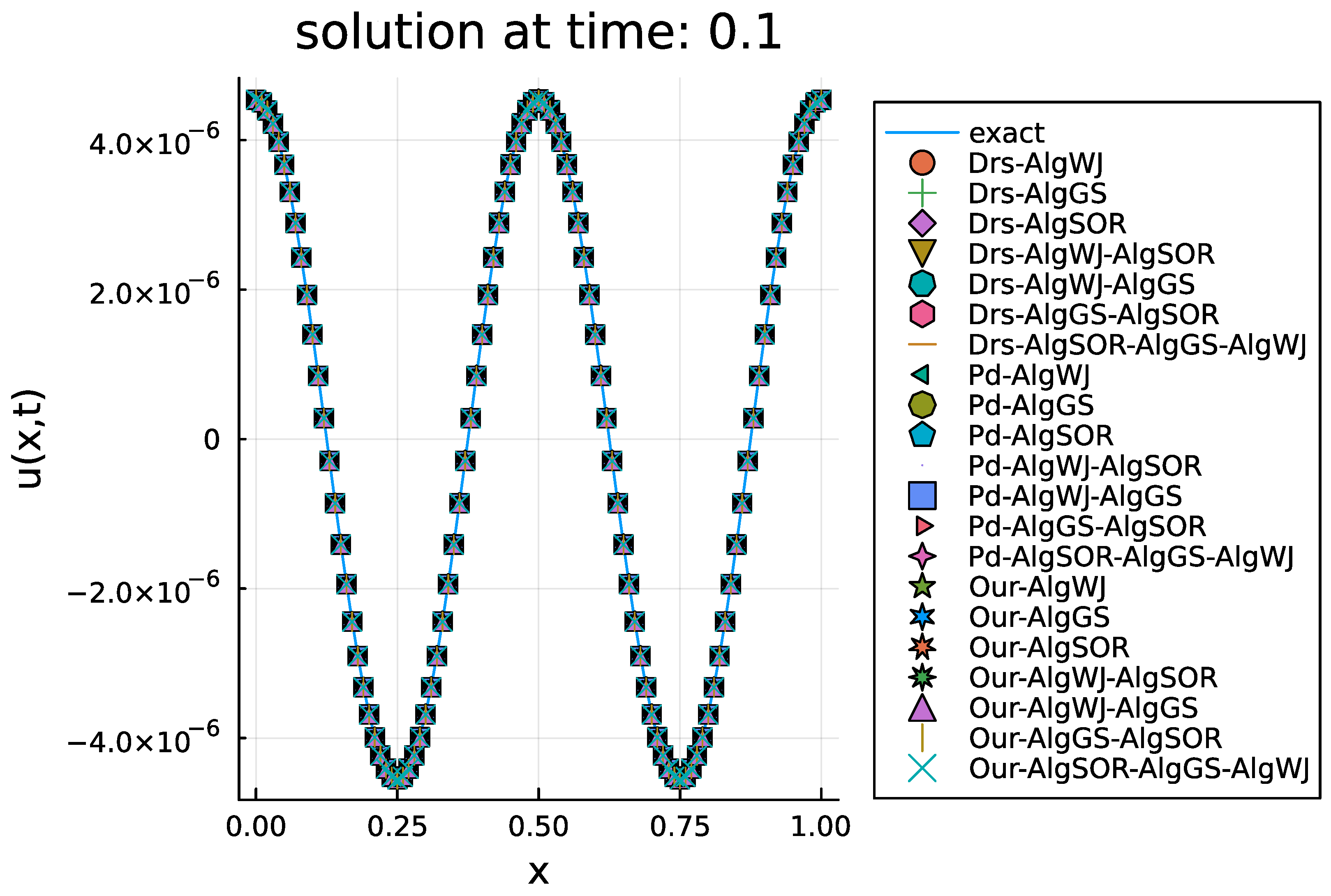
Figure 1 shows the comparison between the exact solution and numerical solutions. To clarify the labels in Figure 1, “Our” refers to our proposed algorithm. In this figure, “Alg” followed by the name of the iterative method, such as WJ, GS, or SOR, represents the fixed point iteration used in the main algorithm for solving linear systems at each time step. We can see from this figure that every method produces almost the same solution. Therefore, our algorithm is capable of solving the linear system effectively.

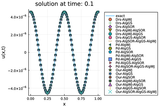
Figure 1. The exact and approximate solutions for the heat equation at time $t=0.1$ and $\Delta x=0.1$.

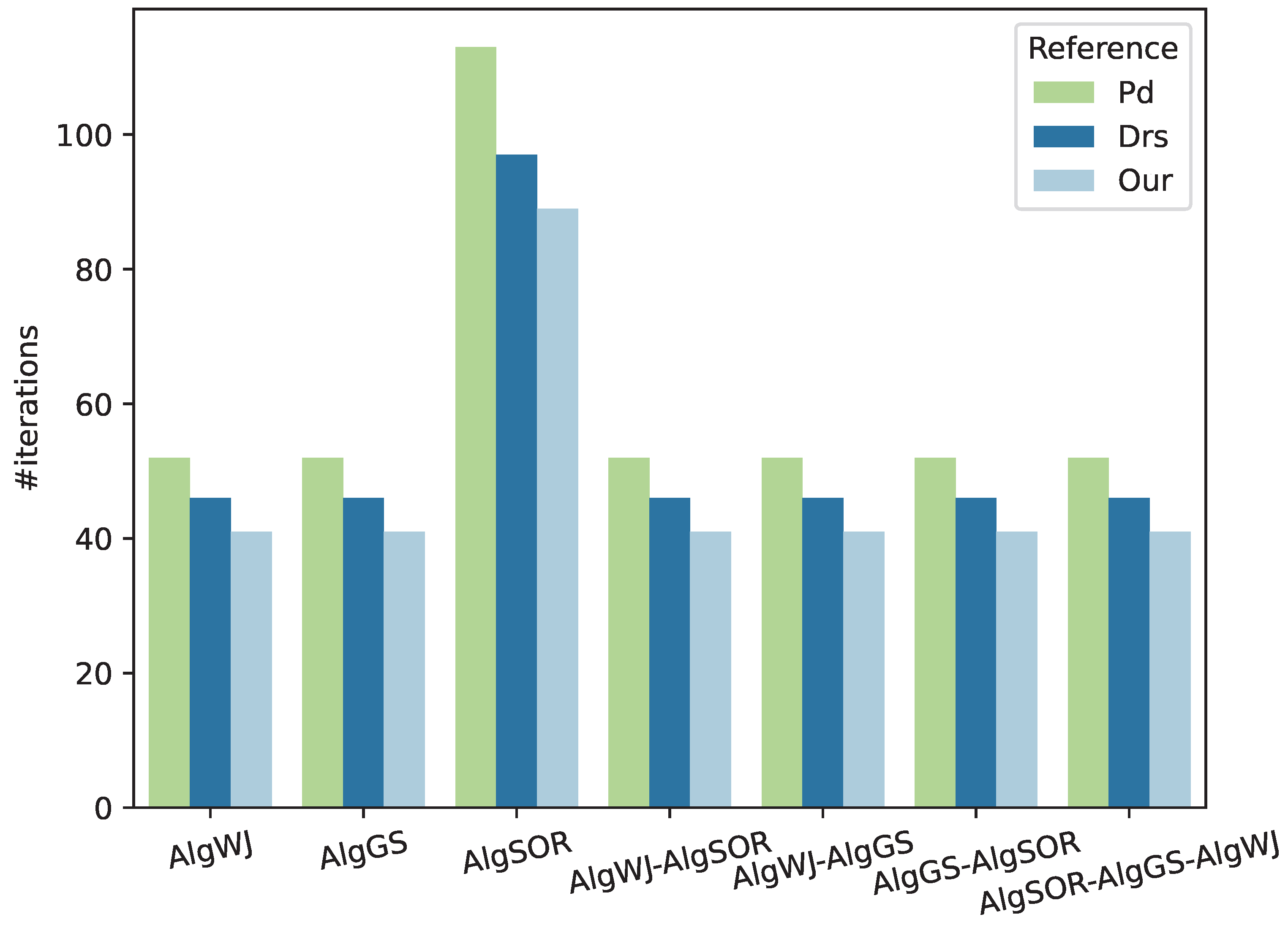
Figure 2 displays a bar plot showing the number of iterations for both the proposed and existing algorithms. The results clearly demonstrate that our algorithm requires fewer iterations to solve the linear system compared to existing algorithms, highlighting the efficiency of our approach. Furthermore, the performance of different fixed point iterations is consistent across each algorithm, suggesting that lower-complexity fixed point iterations can yield the same results. This consistency reduces overall computational time. Additionally, the SOR algorithm, when used alone, has the highest average number of iterations. However, when SOR is combined with another algorithm, the number of iterations decreases to match that of the other algorithm, indicating that SOR is not efficient in this context. Moreover, SOR performs the worst even when combined with other algorithms.

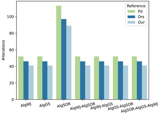
Figure 2. The comparison of the average number of iterations between the literature and our proposed algorithm.

4. Conclusions

This study introduces a novel iterative method for approximating common fixed points of G-nonexpansive mappings in real Hilbert spaces structured by directed graphs. The introduction of left and right coordinate convexity concepts proved crucial in establishing both weak and strong convergence under reasonable assumptions. The proposed algorithm demonstrated its effectiveness in addressing real-world problems, notably in solving the heat equation through linear systems, highlighting its potential application in energy optimization. The results contribute to advancements in computational methods that support sustainable development by offering improved tools for energy-efficient solutions.

References

- Dudorova, N.V.; Belan, B.D. The Energy Model of Urban Heat Island. Atmosphere 2022, 13, 457. [Google Scholar] [CrossRef]
- Allahem, A.; Boulaaras, S.; Zennir, K.; Haiour, M. A new mathematical model of heat equations and its application on the agriculture soil. Eur. J. Pure Appl. Math. 2018, 11, 110–137. [Google Scholar] [CrossRef]
- Ruby, T.; Sutrisno, A. Mathematical modeling of heat transper in agricultural drying machine room (box dryer). J. Phys. Conf. Ser. 2021, 1751, 012029. [Google Scholar] [CrossRef]
- Emmanuel, E.C.; Chinelo, A. On the Numerical Fixed Point Iterative Methods of Solution for the Boundary Value Problems of Elliptic Partial Differential Equation Types. Asian J. Math. Sci. 2018, 2. Available online: https://papers.ssrn.com/sol3/papers.cfm?abstract_id=3812257 (accessed on 29 September 2024).
- Atangana, A.; Araz, S.I. An Accurate Iterative Method for Ordinary Differential Equations with Classical and Caputo-Fabrizio Derivatives; Hindustan Aeronautics Limited: Bangalore, India, 2023. [Google Scholar]
- Young, D. Iterative methods for solving partial difference equations of elliptic type. Trans. Am. Math. Soc. 1954, 76, 92–111. [Google Scholar] [CrossRef]
- Gamboa, J.M.; Gromadzki, G. On the set of fixed points of automorphisms of bordered Klein surfaces. Rev. Mat. Iberoam. 2012, 28, 113–126. [Google Scholar] [CrossRef]
- Cooper, D. Automorphisms of free groups have finitely generated fixed point sets. J. Algebra 1987, 111, 453–456. [Google Scholar] [CrossRef]
- Jachymski, J. The contraction principle for mappings on a metric space with a graph. Proc. Am. Math. Soc. 2008, 136, 1359–1373. [Google Scholar] [CrossRef]
- Aleomraninejad, S.M.A.; Rezapour, S.; Shahzad, N. Some fixed point results on a metric space with a graph. Topol. Its Appl. 2012, 159, 659–663. [Google Scholar] [CrossRef]
- Suparatulatorn, R.; Suantai, S.; Cholamjiak, W. Hybrid methods for a finite family of G-nonexpansive mappings in Hilbert spaces endowed with graphs. AKCE Int. J. Graphs Comb. 2017, 14, 101–111. [Google Scholar] [CrossRef]
- Charoensawan, P.; Yambangwai, D.; Cholamjiak, W.; Suparatulatorn, R. An inertial parallel algorithm for a finite family of G-nonexpansive mappings with application to the diffusion problem. Adv. Differ. Equ. 2021, 2021, 1–13. [Google Scholar] [CrossRef]
- Jun-On, N.; Suparatulatorn, R.; Gamal, M.; Cholamjiak, W. An inertial parallel algorithm for a finite family of G-nonexpansive mappings applied to signal recovery. AIMS Math 2022, 7, 1775–1790. [Google Scholar] [CrossRef]
- Khemphet, A.; Suparatulatorn, R.; Varnakovida, P.; Charoensawan, P. A Modified Parallel Algorithm for a Common Fixed-Point Problem with Application to Signal Recovery. Symmetry 2023, 15, 1464. [Google Scholar] [CrossRef]
- Karahan, I.; Ozdemir, M. A general iterative method for approximation of fixed points and their applications. Adv. Fixed Point Theory 2013, 3, 510–526. [Google Scholar]
- Yambangwai, D.; Thianwan, T. A parallel inertial SP-iteration monotone hybrid algorithm for a finite family of G-nonexpansive mappings and its application in linear system, differential, and signal recovery problems. Carpathian J. Math. 2024, 40, 535–557. [Google Scholar] [CrossRef]
- Van Dung, N.; Trung Hieu, N. Convergence of a new three-step iteration process to common fixed points of three G-nonexpansive mappings in Banach spaces with directed graphs. RACSAM 2020, 114, 140. [Google Scholar] [CrossRef]
- Auslender, A.; Teboulle, M.; Ben-Tiba, S. A Logarithmic-Quadratic Proximal Method for Variational Inequalities. Comput. Optim. Appl. 1999, 12, 31–40. [Google Scholar] [CrossRef]
- Bauschke, H.H.; Combettes, P.L. Convex Analysis and Monotone Operator Theory in Hilbert Spaces; CMS Books in Mathematics; Springer: New York, NY, USA, 2011. [Google Scholar]
- Yambangwai, D.; Cholamjiak, W.; Thianwan, T.; Dutta, H. On a new weight tri-diagonal iterative method and its applications. Soft Comput. 2021, 25, 725–740. [Google Scholar] [CrossRef]
- Bezanson, J.; Karpinski, S.; Shah, V.B.; Edelman, A. Julia: A fast dynamic language for technical computing. arXiv 2012, arXiv:1209.5145. [Google Scholar]
- Bezanson, J.; Edelman, A.; Karpinski, S.; Shah, V.B. Julia: A fresh approach to numerical computing. SIAM Rev. 2017, 59, 65–98. [Google Scholar] [CrossRef]
Disclaimer/Publisher’s Note: The statements, opinions and data contained in all publications are solely those of the individual author(s) and contributor(s) and not of MDPI and/or the editor(s). MDPI and/or the editor(s) disclaim responsibility for any injury to people or property resulting from any ideas, methods, instructions or products referred to in the content. |
© 2024 by the authors. Licensee MDPI, Basel, Switzerland. This article is an open access article distributed under the terms and conditions of the Creative Commons Attribution (CC BY) license (https://creativecommons.org/licenses/by/4.0/).