Elliptic Quaternion Matrices: A MATLAB Toolbox and Applications for Image Processing

Abstract

In this study, we developed a MATLAB 2024a toolbox that performs advanced algebraic calculations in the algebra of elliptic numbers and elliptic quaternions. Additionally, we introduce color image processing methods, such as principal component analysis, image compression, image restoration, and watermarking, based on singular-value decomposition theory for elliptic quaternion matrices; we added these to the newly developed toolbox. The experimental results demonstrate that elliptic quaternionic methods yield better image analysis and processing performance compared to other hypercomplex number-based methods.

1. Introduction

In 1843, Hamilton introduced the concept of real quaternions, expressed as

$$q_{\left(R\right)}=q_{\left(R\right),r}+q_{\left(R\right),i}i+q_{\left(R\right),j}j+q_{\left(R\right),k}k,$$

where $q_{\left(R\right),r}$, $q_{\left(R\right),i}$, $q_{\left(R\right),j}$, and $q_{\left(R\right),k}$ are real-valued components, and the imaginary units i, j, and k satisfy the relations

$$i^2=j^2=k^2=-1,ij=-ji=k,jk=-kj=i,ki=-ik=j.$$

The absence of the commutative property in quaternion multiplication classifies real quaternions as a division ring or, more specifically, a skew field [1]. This mathematical structure finds its application across a broad spectrum of disciplines, including but not limited to quantum mechanics [2], computer graphics [3], signal and image processing [4], and the study of neural networks [5]. In 2005, Sangwine and Bihan introduced a MATLAB toolbox designed to facilitate the computational demands associated with real quaternions and their matrices. This toolbox, notable for its inclusion of image processing functionalities, has been subject to continuous refinement, with its most recent update occurring in February 2024 [6]. MATLAB introduced quaternion support in the R2018b release as part of the Aerospace Toolbox and, after that, incorporated it into several pivotal MATLAB toolboxes such as the Sensor Fusion and Tracking Toolbox, the Robotics System Toolbox, and the Navigation Toolbox. This expansion highlights the importance and applicability of real quaternions in various technological and scientific areas. However, the noncommutative nature of real quaternion multiplication not only introduces certain constraints in various applications but also causes difficulties in calculations. For instance, the inherent complexity in performing the singular-value decomposition of a real quaternion matrix is notably high, registering a computational complexity of $O\left(8n^3\right)$ for an $n\times n$ real quaternion matrix, considering that its complex representation is of size $2n\times 2n$. Additionally, the convolution theorem does not hold for real quaternion-valued signals; that is, the Fourier transform of the convolution products of two such signals does not equate to the dot products of their respective Fourier transforms. This deviation from the convolution theorem implies that the fast Fourier transform algorithm remains undeveloped for real quaternion-valued linear time-invariant systems, presenting challenges in their analysis [7].

As the need for more efficient and versatile algebraic structures grew, researchers sought alternatives to real quaternions that retained the benefits of hypercomplex numbers while mitigating some of the associated limitations. This search led to the development of generalized Segre quaternions, a class of four-dimensional commutative hypercomplex numbers. These quaternions have been gaining attention due to their ability to extend methodologies from the real and complex number domains to more versatile four-dimensional counterparts [8,9]. The definition of generalized Segre quaternions is as follows:

$$q_{\left(\mathrm{GS}\right)}=q_{\left(\mathrm{GS}\right),r}+q_{\left(\mathrm{GS}\right),i}i+q_{\left(\mathrm{GS}\right),j}j+q_{\left(\mathrm{GS}\right),k}k,$$

where $q_{\left(\mathrm{GS}\right),r}, q_{\left(\mathrm{GS}\right),i}, q_{\left(\mathrm{GS}\right),j}, q_{\left(\mathrm{GS}\right),k}\in \mathbb{R}$ and $i,j,k\notin \mathbb{R}$. The multiplication rules for the units $i,j,k$ are given by

$$i^2=k^2=p,j^2=1,ij=ji=k,jk=kj=i,ki=ik=pj,$$

where $p\in \mathbb{R}$. Based on the value of p, generalized Segre quaternions are classified into three categories: hyperbolic quaternions ($p>0$), parabolic quaternions ($p=0$), and elliptic quaternions ($p<0$) [9]. Each of these systems has specific scientific and technological applications. For example, hyperbolic quaternions are used to solve problems in non-Euclidean geometry [10,11], while parabolic quaternions are applied in robotic control and spatial mechanics [10,12]. Due to the elliptic behavior of many physical systems, elliptic quaternions have significant practical applications in applied science. Additionally, elliptic quaternions offer a notable improvement over real quaternions, especially with their commutative multiplication and enhanced generalization capability [9,10,13,14]. These properties result in reduced computational complexity and improved performance across a range of computational tasks. Specifically, the process of singular-value decomposition within the context of elliptic quaternion matrices is characterized by an algorithmic complexity of $O\left(2n^3\right)$, as detailed in [15]. Furthermore, the applicability of the convolution theorem within this mathematical framework enables the formulation of a fast Fourier transform algorithm specifically designed for elliptic quaternion spaces. Consequently, recent developments in elliptic quaternion-valued methodologies have demonstrated their superiority over conventional real quaternion approaches in critical fields such as image processing, signal processing, and deep learning, as evidenced by [7,14,15,16,17].

In this paper, we present a MATLAB toolbox that we developed for performing advanced calculations in elliptic numbers and elliptic quaternions. The aim of this toolbox is to address and provide solutions to the computational challenges associated with these algebraic structures, thereby facilitating further scientific and technological research in this field. This development is fundamentally rooted in the theoretical framework and algorithms delineated in references [9,15,18]. Furthermore, by leveraging mathematical theory and algorithms elucidated in [15], we have enriched this toolbox with advanced color image processing methodologies, including but not limited to principal component analysis, image compression, image restoration, and watermarking techniques. We have observed that the proposed methods for image compression, image restoration, and watermarking exhibit better performance than existing techniques based on separable, real quaternions and reduced biquaternions (for comparison results, see Tables 4–8). Moreover, our performance analyses reveal that the p-value of elliptic quaternions directly affects the solution of the problem, with better results obtained by adjusting this p-value (for optimal p-value results, see Figures 11, 13 and 19).

Within the context of this paper, the following notations are employed. Let $\mathbb{R}$, $\mathbb{C}$, ${\mathbb{C}}_p$, and ${\mathbb{H}}_p$ denote the sets of real numbers, complex numbers, elliptic numbers, and elliptic quaternions, respectively. ${\mathbb{R}}^{m\times n}$, ${\mathbb{C}}^{m\times n}$, ${\mathbb{C}}_p^{m\times n}$, and ${\mathbb{H}}_p^{m\times n}$ denote the set of all $m\times n$ matrices on $\mathbb{R}$, $\mathbb{C}$, ${\mathbb{C}}_p$, and ${\mathbb{H}}_p$, respectively. Throughout the study, we use the following notations: $q_{\left(\square \right)}$ represents a complex number when $\square =c$, an elliptic number when $\square =e$, and an elliptic quaternion when $\square =E$. Similarly, $Q_{\left(\square \right)}$ denotes a complex matrix when $\square =c$, an elliptic matrix when $\square =e$, and an elliptic quaternion matrix when $\square =E$. This study was conducted using MATLAB 2024a (64-bit) on a system equipped with an Intel^® Raptor Lake Core™ i7-13700H 14C/20T, NVIDIA^® GeForce^® RTX4060 and 32 GB of DDR5 RAM.

2. Mathematical Preliminaries

This section establishes the fundamental algebraic properties and the notations for elliptic numbers and elliptic quaternions.

2.1. Elliptic Numbers

An elliptic number $q_{\left(e\right)}$ is denoted by $q_{\left(e\right)}=q_{\left(e\right),r}+q_{\left(e\right),i}i$, where $i^2=p<0$ and $q_{\left(e\right),r},q_{\left(e\right),i},p\in \mathbb{R}$. The conjugate and norm of $q_{\left(e\right)}\in {\mathbb{C}}_p$ are defined as $\overline{q_{\left(e\right)}}=q_{\left(e\right),r}-q_{\left(e\right),i}i\mathrm{and}{∥q_{\left(e\right)}∥}_p=\sqrt{q_{\left(e\right),r}^2-p{q}_{\left(e\right),i}^2},$ respectively [19]. The multiplication of the elliptic numbers $q_{1,\left(e\right)}=q_{1,\left(e\right),r}+q_{1,\left(e\right),i}i$ and $q_{2,\left(e\right)}=q_{2,\left(e\right),r}+q_{2,\left(e\right),i}i$ is defined as

$$q_{1,\left(e\right)}{q}_{2,\left(e\right)}=\left(q_{1,\left(e\right),r}{q}_{2,\left(e\right),r}+p{q}_{1,\left(e\right),i}{q}_{2,\left(e\right),i}\right)+i\left(q_{1,\left(e\right),r}{q}_{2,\left(e\right),i}+q_{2,\left(e\right),r}{q}_{1,\left(e\right),i}\right).$$

An elliptic matrix $Q_{\left(e\right)}$ is denoted as $Q_{\left(e\right)}=Q_{\left(e\right),r}+Q_{\left(e\right),i}i$, where $i^2=p<0$, $p\in \mathbb{R}$, and $Q_{\left(e\right),r}$, $Q_{\left(e\right),i}\in {\mathbb{R}}^{m\times n}$. The conjugate, transpose, conjugate transpose, and Frobenius norm of $Q_{\left(e\right)}\in {\mathbb{C}}_p^{m\times n}$ are defined by $\overline{Q_{\left(e\right)}}=Q_{\left(e\right),r}-Q_{\left(e\right),i}i$, $Q_{\left(e\right)}^T=Q_{\left(e\right),r}^T+Q_{\left(e\right),i}^{T}i,Q_{\left(e\right)}^{*}=Q_{\left(e\right),r}^T-Q_{\left(e\right),i}^{T}i,$ and $\parallel Q_{\left(e\right)}{\parallel }_p = \sqrt{\parallel Q_{\left(e\right),r}{\parallel }^2 - p{\parallel Q_{\left(e\right),i}\parallel }^2}$, respectively [15,19]. The multiplication of two elliptic matrices $Q_{1,\left(e\right)}=Q_{1,\left(e\right),r}+Q_{1,\left(e\right),i}i$ and $Q_{2,\left(e\right)}=Q_{2,\left(e\right),r}+Q_{2,\left(e\right),i}i$ is defined as

$$Q_{1,\left(e\right)}{Q}_{2,\left(e\right)}=\left(Q_{1,\left(e\right),r}{Q}_{2,\left(e\right),r}+p{Q}_{1,\left(e\right),i}{Q}_{2,\left(e\right),i}\right)+i\left(Q_{1,\left(e\right),r}{Q}_{2,\left(e\right),i}+Q_{2,\left(e\right),r}{Q}_{1,\left(e\right),i}\right).$$

There exists an isomorphism between elliptic matrices and complex matrices, as depicted in the following:

$$\begin{array}{c}{\mathrm{H}}_p:{\mathbb{C}}_p^{m\times n}\to {\mathbb{C}}^{m\times n}\hfill \\ Q_{\left(e\right)}=Q_{\left(e\right),r}+Q_{\left(e\right),i}i\to {\mathrm{H}}_p\left(Q_{\left(e\right)}\right)=Q_{\left(c\right)}=Q_{\left(e\right),r}+I\sqrt{-p}{Q}_{\left(e\right),i},\hfill \end{array}$$

where I represents the complex unit ($I^2=-1$) [15].

Lemma 1

([15]). Let the eigenvalues of a complex matrix ${\mathrm{H}}_p\left(Q_{\left(e\right)}\right)$ be denoted by ${\lambda }_{{\mathrm{H}}_p\left(Q_{\left(e\right)}\right)}$, and let the corresponding eigenvectors be represented by $x_{{\mathrm{H}}_p\left(Q_{\left(e\right)}\right)}.$ Then, the eigenvalues of the elliptic matrix $Q_{\left(e\right)}\in {\mathbb{C}}_p^{n\times n}$ are given by

$${\lambda }_{(e)}=Re({\lambda }_{{\mathrm{H}}_p(Q_{(e)})})+{\displaystyle \frac{i}{\sqrt{-p}}}Im({\lambda }_{{\mathrm{H}}_p(Q_{(e)})})$$

and the corresponding eigenvectors are given by

$$x_{(e)}=Re(x_{{\mathrm{H}}_p(Q_{(e)})})+{\displaystyle \frac{i}{\sqrt{-p}}}Im(x_{{\mathrm{H}}_p(Q_{(e)})}).$$

Lemma 2

([15]). Let $Q_{\left(e\right)}\in {\mathbb{C}}_p^{m\times n}$. The pseudoinverse of $Q_{\left(e\right)}$ is given by

$${\left(Q_{\left(e\right)}\right)}^{†}=\mathrm{Re}\left({\left({\mathrm{H}}_{\mathrm{p}}\left(Q_{\left(e\right)}\right)\right)}^{†}\right)+{\displaystyle \frac{i}{\sqrt{-p}}}\mathrm{Im}\left({\left({\mathrm{H}}_{\mathrm{p}}\left(Q_{\left(e\right)}\right)\right)}^{†}\right),$$

where ${\left({\mathrm{H}}_{\mathrm{p}}\left(Q_{\left(e\right)}\right)\right)}^{†}$ is the pseudoinverse of the complex matrix ${\mathrm{H}}_{\mathrm{p}}\left({\mathrm{Q}}_{\left(\mathrm{e}\right)}\right)$.

Lemma 3

([15]). Let $Q_{\left(e\right)}\in {\mathbb{C}}_p^{m\times n}$. Suppose that the singular-value decomposition of the complex matrix ${\mathrm{H}}_p\left(Q_{\left(e\right)}\right)$ is given by ${\mathrm{H}}_{\mathrm{p}}\left(Q_{\left(e\right)}\right)=U_{\left(c\right)}\mathsf{\Sigma }{V}_{\left(c\right)}^{*}.$ Then, the singular-value decomposition of the elliptic matrix $Q_{\left(e\right)}$ is $Q_{\left(e\right)}=U_{\left(e\right)}\mathsf{\Sigma }{V}_{\left(e\right)}^{*},$ where

$$U_{\left(e\right)}=\left(Re\left(U_{\left(c\right)}\right)+{\displaystyle \frac{i}{\sqrt{-p}}}Im\left(U_{\left(c\right)}\right)\right)and{V}_{\left(e\right)}=\left(Re\left(U_{\left(c\right)}\right)+{\displaystyle \frac{i}{\sqrt{-p}}}Im\left(U_{\left(c\right)}\right)\right).$$

Lemma 4

([15]). Let $Q_{1,\left(e\right)}\in {\mathbb{C}}_p^{m\times n}$ and $Q_{2,\left(e\right)}\in {\mathbb{C}}_p^{m\times q}$. Suppose that ${\mathrm{H}}_{\mathrm{p}}\left(Q_{1,\left(e\right)}\right)=U_{\left(c\right)}\mathsf{\Sigma }{V}_{\left(c\right)}^{*}.$ In this case, the least squares solution with the minimum norm $X_{\left(e\right)}$ of the elliptic matrix equation $Q_{1,\left(e\right)}{X}_{\left(e\right)}=Q_{2,\left(e\right)}$ is given by

$$X_{\left(e\right)}=\left(\mathrm{Re}\left(V_{\left(e\right)}\right)+{\displaystyle \frac{i}{\sqrt{-p}}}\mathrm{Im}\left(V_{\left(e\right)}\right)\right){\mathsf{\Sigma }}^{†}{\left(\mathrm{Re}\left(U_{\left(e\right)}\right)+{\displaystyle \frac{i}{\sqrt{-p}}}\mathrm{Im}\left(U_{\left(e\right)}\right)\right)}^{*}{Q}_{2,\left(e\right)}.$$

2.2. Elliptic Quaternions

An elliptic quaternion $q_{\left(E\right)}$ is denoted as $q_{\left(E\right)}=q_{\left(E\right),r}+q_{\left(E\right),i}i+q_{\left(E\right),j}j+q_{\left(E\right),k}k$, where $i^2=k^2=p<0$, $j^2=1$, $ij=ji=k$, $jk=kj=i$, $ki=ik=pj$, and $q_{\left(E\right),r}, q_{\left(E\right),i}, q_{\left(E\right),j}, q_{\left(E\right),k}, p\in \mathbb{R}$. An elliptic quaternion $q_{\left(E\right)}$ is denoted in the following forms:

$$q_{\left(E\right)}=\left(q_{\left(E\right),r}+i{q}_{\left(E\right),i}\right)+\left(q_{\left(E\right),j}+i{q}_{\left(E\right),k}\right)j=q_{\left(e\right),1}{e}_1+q_{\left(e\right),2}{e}_2,$$

where

$$q_{\left(e\right),1}=\left(q_{\left(E\right),r}+q_{\left(E\right),j}\right)+\left(q_{\left(E\right),i}+q_{\left(E\right),k}\right)i$$

and

$$q_{\left(e\right),2}=\left(q_{\left(E\right),r}-q_{\left(E\right),j}\right)+\left(q_{\left(E\right),i}-q_{\left(E\right),k}\right)i$$

are elliptic numbers and $e_1={\displaystyle \frac{1+j}{2}}$ and $e_2={\displaystyle \frac{1-j}{2}}.$ Clearly, $e_1{e}_2=0$, $e_1+e_2=1$, $e_1-e_2=j$ and $e_1^2=e_1,e_2^2=e_2.$ As a result, $e_1$ and $e_2$ are disjoint idempotent units.

The multiplication of the two elliptic quaternions $q_{1,\left(E\right)}=q_{1,\left(e\right),1}{e}_1+q_{1,\left(e\right),2}{e}_2$ and $q_{2,\left(E\right)}=q_{2,\left(e\right),1}{e}_1+q_{2,\left(e\right),2}{e}_2$ is defined by

$$\begin{array}{c}{q}_{1,\left(E\right)}{q}_{2,\left(E\right)}=\left(q_{1,\left(e\right),1}{q}_{2,\left(e\right),1}\right)e_1+\left(q_{1,\left(e\right),2}{q}_{2,\left(e\right),2}\right)e_2.\hfill \end{array}$$

The conjugate and norm of the elliptic quaternion $q_{\left(E\right)}=q_{\left(e\right),1}{e}_1+q_{\left(e\right),2}{e}_2$ are defined by $\overline{q_{\left(E\right)}}=\overline{q_{\left(e\right),1}}{e}_1+\overline{q_{\left(e\right),2}}{e}_2$ and ${∥q_{\left(E\right)}∥}_p={\displaystyle \frac{1}{\sqrt{2}}}\sqrt{\left({∥q_{\left(e\right),1}∥}_p^2+{∥q_{\left(e\right),2}∥}_p^2\right)},$ respectively [10].

An elliptic quaternion matrix $Q_{\left(E\right)}$ is represented

$$\begin{array}{c}{Q}_{\left(E\right)}=Q_{\left(E\right),r}+Q_{\left(E\right),i}i+Q_{\left(E\right),j}j+Q_{\left(E\right),k}k=\left(Q_{\left(E\right),r}+Q_{\left(E\right),i}i\right)+\left(Q_{\left(E\right),j}+Q_{\left(E\right),k}i\right)j\hfill \\ =Q_{\left(e\right),1}{e}_1+Q_{\left(e\right),2}{e}_2,\hfill \end{array}$$

where

$$Q_{\left(e\right),1}=\left(Q_{\left(E\right),r}+Q_{\left(E\right),j}\right)+\left(Q_{\left(E\right),i}+Q_{\left(E\right),k}\right)i$$

and

$$Q_{\left(e\right),2}=\left(Q_{\left(E\right),r}-Q_{\left(E\right),j}\right)+\left(Q_{\left(E\right),i}-Q_{\left(E\right),k}\right)i$$

are elliptic matrices, and $Q_{\left(E\right),r},Q_{\left(E\right),i},Q_{\left(E\right),j},Q_{\left(E\right),k}\in {\mathbb{R}}^{m\times n}$. The multiplication of the two elliptic quaternion matrices $Q_{1,\left(E\right)}=Q_{1,\left(e\right),1}{e}_1+Q_{1,\left(e\right),2}{e}_2$ and $Q_{2,\left(E\right)}=Q_{2,\left(e\right),1}{e}_1+Q_{2,\left(e\right),2}{e}_2$ is defined by

$$\begin{array}{c}{Q}_{1,\left(E\right)}{Q}_{2,\left(E\right)}=\left(Q_{1,\left(e\right),1}{Q}_{2,\left(e\right),1}\right)e_1+\left(Q_{1,\left(e\right),2}{Q}_{2,\left(e\right),2}\right)e_2.\hfill \end{array}$$

The conjugate, transpose, conjugate transpose, and Frobenius norm of elliptic quaternion matrix $Q_{\left(E\right)}=Q_{\left(e\right),1}{e}_1+Q_{\left(e\right),2}{e}_2\in {\mathbb{H}}_p^{m\times n}$ are defined by $\overline{Q_{\left(E\right)}}=\overline{Q_{\left(e\right),1}}{e}_1+\overline{Q_{\left(e\right),2}}{e}_2$, $Q_{\left(E\right)}^T=Q_{\left(e\right),1}^T{e}_1+Q_{\left(e\right),2}^T{e}_2$, $Q_{\left(E\right)}^{*}=\overline{Q_{\left(e\right),1}^T}{e}_1+\overline{Q_{\left(e\right),2}^T}{e}_2$ and ${∥Q_{\left(E\right)}∥}_p={\displaystyle \frac{1}{\sqrt{2}}}\sqrt{{∥Q_{\left(e\right),1}∥}_p^2+{∥Q_{\left(e\right),2}∥}_p^2},$ respectively [18,20].

Theorem 1

([15]). Let $Q_{\left(E\right)}=Q_{\left(e\right),1}{e}_1+Q_{\left(e\right),2}{e}_2\in {\mathbb{H}}_p^{n\times n}$. Suppose that ${\lambda }_{\left(e\right),1}$ and ${\lambda }_{\left(e\right),2}$ are eigenvalues of elliptic matrices $Q_{\left(e\right),1}$ and $Q_{\left(e\right),2}$ corresponding to the eigenvectors $x_{\left(e\right),1}$ and $x_{\left(e\right),2},$ respectively. Then, ${\lambda }_{\left(E\right)}={\lambda }_{\left(e\right),1}{e}_1+{\lambda }_{\left(e\right),2}{e}_2$ is an eigenvalue of $Q_{\left(E\right)}$ corresponding to the eigenvector $x_{\left(E\right)}=x_{\left(e\right),1}{e}_1+x_{\left(e\right),2}{e}_2$.

Theorem 2

([15]). Let $Q_{\left(E\right)}=Q_{\left(e\right),1}{e}_1+Q_{\left(e\right),2}{e}_2\in {\mathbb{H}}_p^{m\times n}$. Suppose that singular-value decompositions of $Q_{\left(e\right),1}$ and $Q_{\left(e\right),2}$ are $Q_{\left(e\right),1}=U_{\left(e\right),1}{\mathsf{\Sigma }}_1{V}_{\left(e\right),1}^{*}$ and $Q_{\left(e\right),2}=U_{\left(e\right),2}{\mathsf{\Sigma }}_2{V}_{\left(e\right),2}^{*}$, respectively. Then, the singular-value decomposition of the elliptic quaternion matrix $Q_{\left(E\right)}$ is given by $Q_{\left(E\right)}=U_{\left(E\right)}{\mathsf{\Sigma }}_{\left(E\right)}{V}_{\left(E\right)}^{*},$ where ${\mathsf{\Sigma }}_{\left(E\right)}={\mathsf{\Sigma }}_1{e}_1+{\mathsf{\Sigma }}_2{e}_2$ is hyperbolic matrix since ${\mathsf{\Sigma }}_1$ and ${\mathsf{\Sigma }}_2$ are real matrices (${\mathsf{\Sigma }}_{\left(E\right)}$ is real matrix if and only if ${\mathsf{\Sigma }}_1={\mathsf{\Sigma }}_2$). Moreover $U_{\left(E\right)}=U_{\left(e\right),1}{e}_1+U_{\left(e\right),2}{e}_2$ and $V_{\left(E\right)}=V_{\left(e\right),1}{e}_1+V_{\left(e\right),2}{e}_2$ are unitary matrices.

Corollary 1

([15]). Let $Q_{\left(E\right)}=Q_{\left(e\right),1}{e}_1+Q_{\left(e\right),2}{e}_2\in {\mathbb{H}}_p^{m\times n}$ and $Q_{\left(E\right)}=U_{\left(E\right)}{\mathsf{\Sigma }}_{\left(E\right)}{V}_{\left(E\right)}^{*}.$ Then, the pseudoinverse of $Q_{\left(E\right)}$ is $Q_{\left(E\right)}^{†}=V_{\left(E\right)}{\mathsf{\Sigma }}_{\left(E\right)}^{†}{U}_{\left(E\right)}^{*}$, where ${\mathsf{\Sigma }}_{\left(E\right)}^{†}={\mathsf{\Sigma }}_1^{†}{e}_1+{\mathsf{\Sigma }}_2^{†}{e}_2$ and ${\mathsf{\Sigma }}_1,{\mathsf{\Sigma }}_2\in {\mathbb{R}}^{m\times n}.$

Theorem 3

([15]). The least squares solution with the minimum norm of the elliptic quaternion matrix equation $Q_{1,\left(E\right)}{X}_{\left(E\right)}=Q_{2,\left(E\right)}$ is $X_{\left(E\right)}=Q_{1,\left(E\right)}^{†}{Q}_{2,\left(E\right)}=V_{\left(E\right)}{\mathsf{\Sigma }}_{\left(E\right)}^{†}{U}_{\left(E\right)}^{*}{Q}_{2,\left(E\right)},$ where $Q_{1,\left(E\right)}\in {\mathbb{H}}_p^{m\times n}$ and $Q_{2,\left(E\right)}\in {\mathbb{H}}_p^{m\times q}$.

3. MATLAB Toolbox for Elliptic Numbers and Elliptic Quaternions

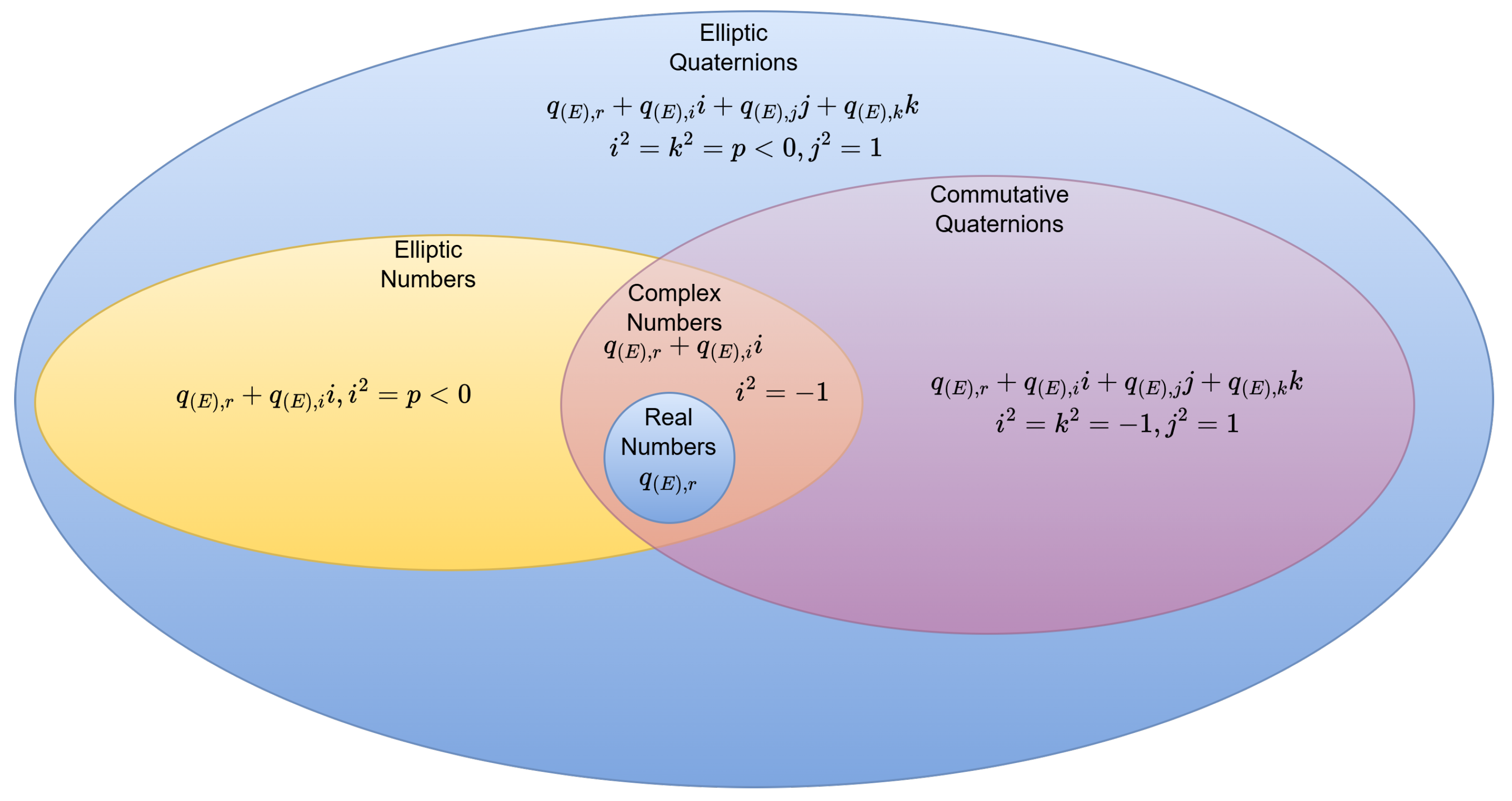
Elliptic numbers and elliptic quaternions are number systems that confer significant advantages in solving certain mathematical and physical problems. In this section, we introduce a MATLAB toolbox (version 0.1) developed to facilitate computations involving these systems. As illustrated in Figure 1, elliptic quaternions generalize elliptic numbers, reduced biquaternions (commutative quaternions), complex numbers, and real numbers, thereby providing a more expansive computational framework. This generalization enhances the versatility and applicability of the developed toolbox.

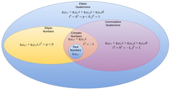
Figure 1. The set of elliptic quaternions and the number sets it contains.

Table 1 and Table 2 show the signatures and their descriptions of the functions of the elliptic numbers and elliptic quaternions, respectively, in the toolbox.

Table 1. Key functions of the elliptic numbers.

Function Name	Description
ellipticcomplex2complexnumber($q_{\left(e\right)}$)	Returns the complex number (or matrix) to which the elliptic number (or matrix) is isomorphic.
complexnumber2ellipticcomplex($p$-value, complex)	Returns the elliptic number (or matrix) to which the complex number (or matrix) is isomorphic.
elliptic_n_addition($q_{\left(e\right)}$,$p_{\left(e\right)}$)	Returns the sum of two elliptic numbers (or matrices).
elliptic_n_subtraction($q_{\left(e\right)}$,$p_{\left(e\right)}$)	Returns the difference of two elliptic numbers (or matrices).
elliptic_n_product($q_{\left(e\right)}$,$p_{\left(e\right)}$)	Returns the product of two elliptic numbers (or matrices).
elliptic_n_transpose($Q_{\left(e\right)}$)	Returns the transpose of the elliptic matrix $Q_{\left(e\right)}$.
elliptic_n_conjugate($Q_{\left(e\right)}$)	Returns the conjugate of the elliptic matrix $Q_{\left(e\right)}$.
elliptic_n_hermitianconjugate($Q_{\left(e\right)}$)	Returns the Hermitian conjugate of the elliptic matrix $Q_{\left(e\right)}$.
elliptic_n_eig($Q_{\left(e\right)}$)	[$D_{\left(e\right)}$,$V_{\left(e\right)}$] = elliptic_n_eig($Q_{\left(e\right)}$) returns diagonal matrix $D_{\left(e\right)}$ of eigenvalues and matrix $V_{\left(e\right)}$ whose columns are the corresponding eigenvectors, so that $Q_{\left(e\right)}{V}_{\left(e\right)}=V_{\left(e\right)}{D}_{\left(e\right)}$.
elliptic_n_svd($Q_{\left(e\right)}$)	[$U_e$,$S_e$,$V_e$] = elliptic_n_svd($Q_{\left(e\right)}$) performs a singular-value decomposition of elliptic matrix $Q_{\left(e\right)}$, such that $Q_{\left(e\right)}=U_{\left(e\right)}{S}_{\left(e\right)}{V}_{\left(e\right)}^{*}$.
elliptic_n_pinv($Q_{\left(e\right)}$)	Returns the pseudoinverse of the elliptic matrix $Q_{\left(e\right)}$.
elliptic_n_rank($Q_{\left(e\right)}$)	Returns the rank of the elliptic matrix $Q_{\left(e\right)}$.
elliptic_n_lss($Q_{\left(e\right)},P_{\left(e\right)}$)	Returns the least squares solution of the elliptic matrix equation $Q_{\left(e\right)}{X}_{\left(e\right)}=P_{\left(e\right)}$ and the least squares error.

Table 2. Key functions of the elliptic quaternions.

Function Name	Description
e1e2form($q_{\left(E\right)}$)	Returns the elliptic quaternion (or elliptic quaternion matrix) given in ijk-form in $e_1$-$e_2$ form.
ijkform(e1_part,e2_part)	Returns the elliptic quaternion (or elliptic quaternion matrix) given in $e_1$-$e_2$ form in ijk form.
elliptic_q_conjugate_1($q_{\left(E\right)}$)	Returns the 1st conjugate of the elliptic quaternion (or elliptic quaternion matrix).
elliptic_q_conjugate_2($q_{\left(E\right)}$)	Returns the 2nd conjugate of the elliptic quaternion (or elliptic quaternion matrix).
elliptic_q_conjugate_3($q_{\left(E\right)}$)	Returns the 3rd conjugate of the elliptic quaternion (or elliptic quaternion matrix).
elliptic_q_addition($q_{\left(E\right)}$,$p_{\left(E\right)}$)	Returns the sum of two elliptic quaternions (or elliptic quaternion matrices).
elliptic_q_subtraction($q_{\left(E\right)}$,$p_{\left(E\right)}$)	Returns the difference of two elliptic quaternions (or elliptic quaternion matrices).
elliptic_q_product($q_{\left(E\right)}$,$p_{\left(E\right)}$)	Returns the product of two elliptic quaternions (or elliptic quaternion matrices).
elliptic_q_scalar(lamda,$q_{\left(E\right)}$)	Returns the lambda scalar multiple of the elliptic quaternion (or elliptic quaternion matrix).
elliptic_q_norm($q_{\left(E\right)}$)	Returns the norm of the elliptic quaternion (or elliptic quaternion matrix).
elliptic_q_transpose($Q_{\left(E\right)}$)	Returns the transpose of the elliptic quaternion matrix.
elliptic_q_hermitianconjugate($Q_{\left(E\right)}$)	Returns the conjugate transpose of the elliptic quaternion matrix.
elliptic_q_eig($Q_{\left(E\right)}$)	[$D_{\left(E\right)}$,$V_{\left(E\right)}$] = elliptic_q_eig($Q_{\left(E\right)}$) returns diagonal matrix $D_{\left(E\right)}$ of eigenvalues and matrix $V_{\left(E\right)}$ whose columns are the corresponding eigenvectors, so that $Q_{\left(E\right)}{V}_{\left(E\right)}=V_{\left(E\right)}{D}_{\left(E\right)}$.
elliptic_q_svd($Q_{\left(E\right)}$)	[$U_{\left(E\right)}$,$S_{\left(E\right)}$,$V_{\left(E\right)}$] = elliptic_q_svd($Q_{\left(E\right)}$) performs a singular-value decomposition of elliptic quaternion matrix $Q_{\left(E\right)}$, such that $Q_{\left(E\right)}=U_{\left(E\right)}{S}_{\left(E\right)}{V}_{\left(E\right)}^{*}$.
elliptic_q_pseudoinverse($Q_{\left(E\right)}$)	Returns the pseudoinverse of the elliptic quaternion matrix.
elliptic_q_lss($Q_{\left(E\right)}$,$P_{\left(E\right)}$)	Returns the least squares solution of the elliptic quaternion matrix equation $Q_{\left(E\right)}{X}_{\left(E\right)}=P_{\left(E\right)}$ and the least squares error.
elliptic_q_qrank($Q_{\left(E\right)}$)	Returns the rank of the elliptic matrix.

To enable the toolbox to process any elliptic number, the user must specify its real part, imaginary part, and the associated p-value. For example, to initialize the elliptic number $q_{\left(e\right)}=1+2i$ and the elliptic matrix $Q_{\left(e\right)}\in {\mathbb{C}}_{-5}^{3\times 3}$ (initialized with random numbers) for $p=-5$, the functions in the Listing 1 should be invoke.

Listing 1. MATLAB console output of the function elliptic_number().

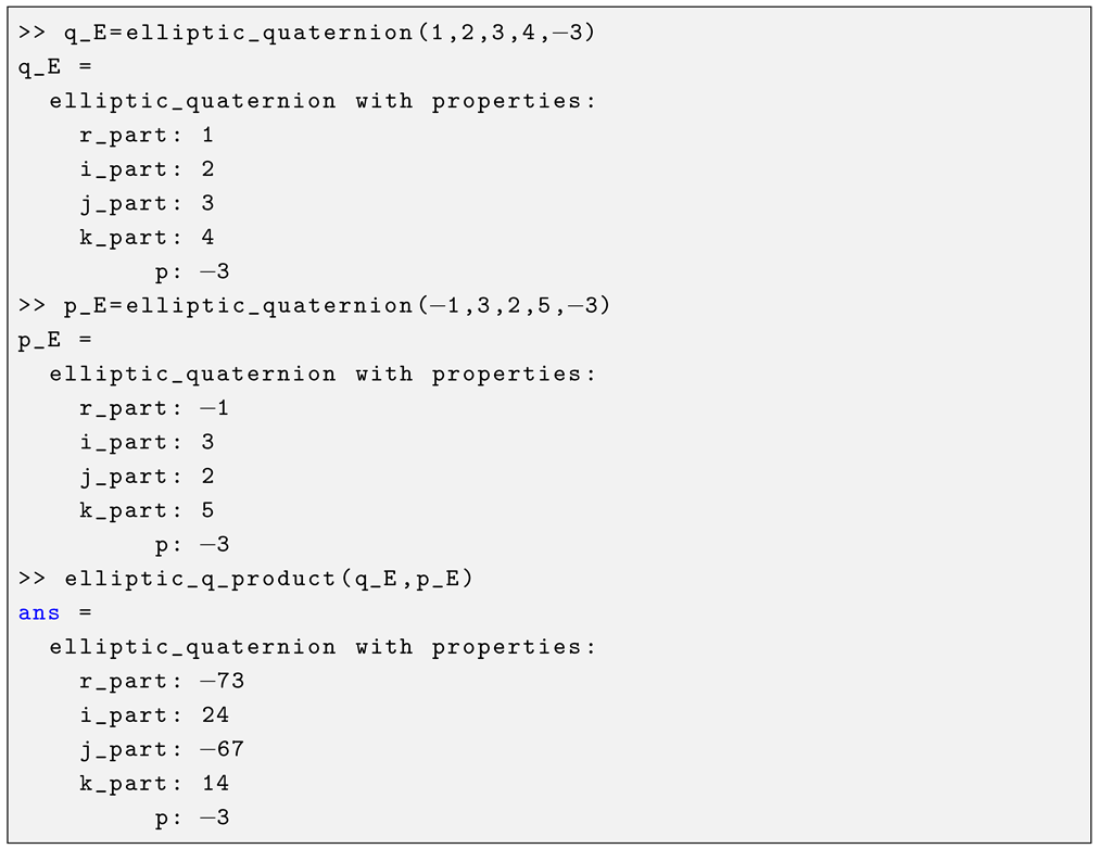
Initializing the elliptic quaternions $q_{\left(E\right)}=1+2i+3j+4k$ and $p_{\left(E\right)}=-1+3i+2j+5k$ for $p=-3$ and their multiplication is carried out as in the Listing 2:

Listing 2. MATLAB console output of the functions elliptic_quaternion() and elliptic_q_product().

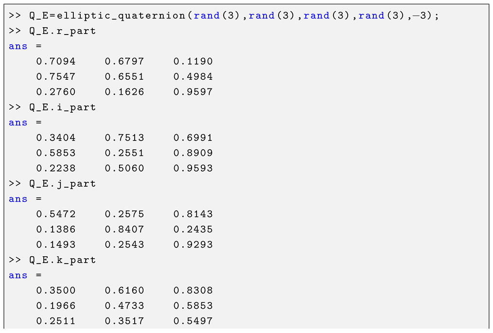
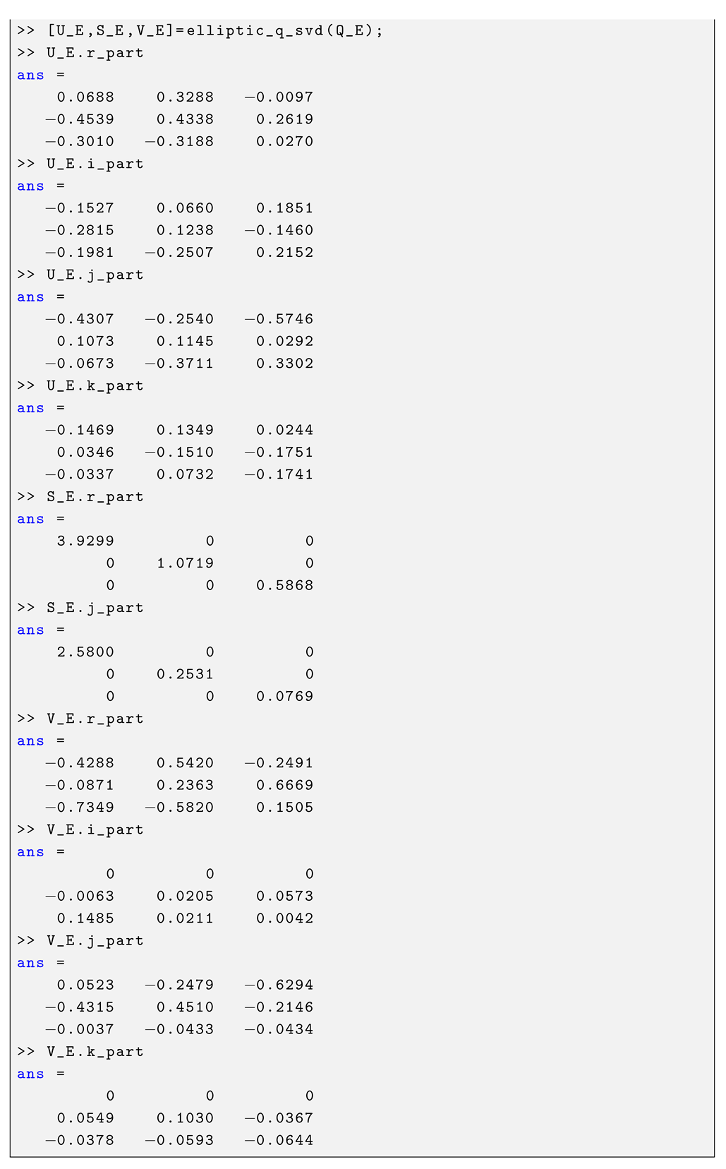
The singular-value decomposition of the elliptic quaternion matrix $Q_{\left(E\right)}\in {\mathbb{H}}_{-3}^{3\times 3}$, initialized with random numbers for $p=-3$, is conducted as in the Listing 3:

Listing 3. MATLAB console output of the functions elliptic_quaternion() and elliptic_q_svd().

The minimum error and least squares solution of the matrix equation $Q_{\left(E\right)}{X}_{\left(E\right)}=P_{\left(E\right)}$, where $P_{\left(E\right)}\in {\mathbb{H}}_{-3}^{3\times 5}$ is initialized with random numbers for $p=-3$, are carried out as in the Listing 4:

Listing 4. MATLAB console output of the functions elliptic_quaternion() and elliptic_q_lss().

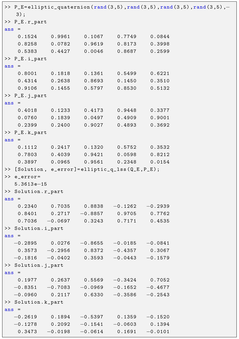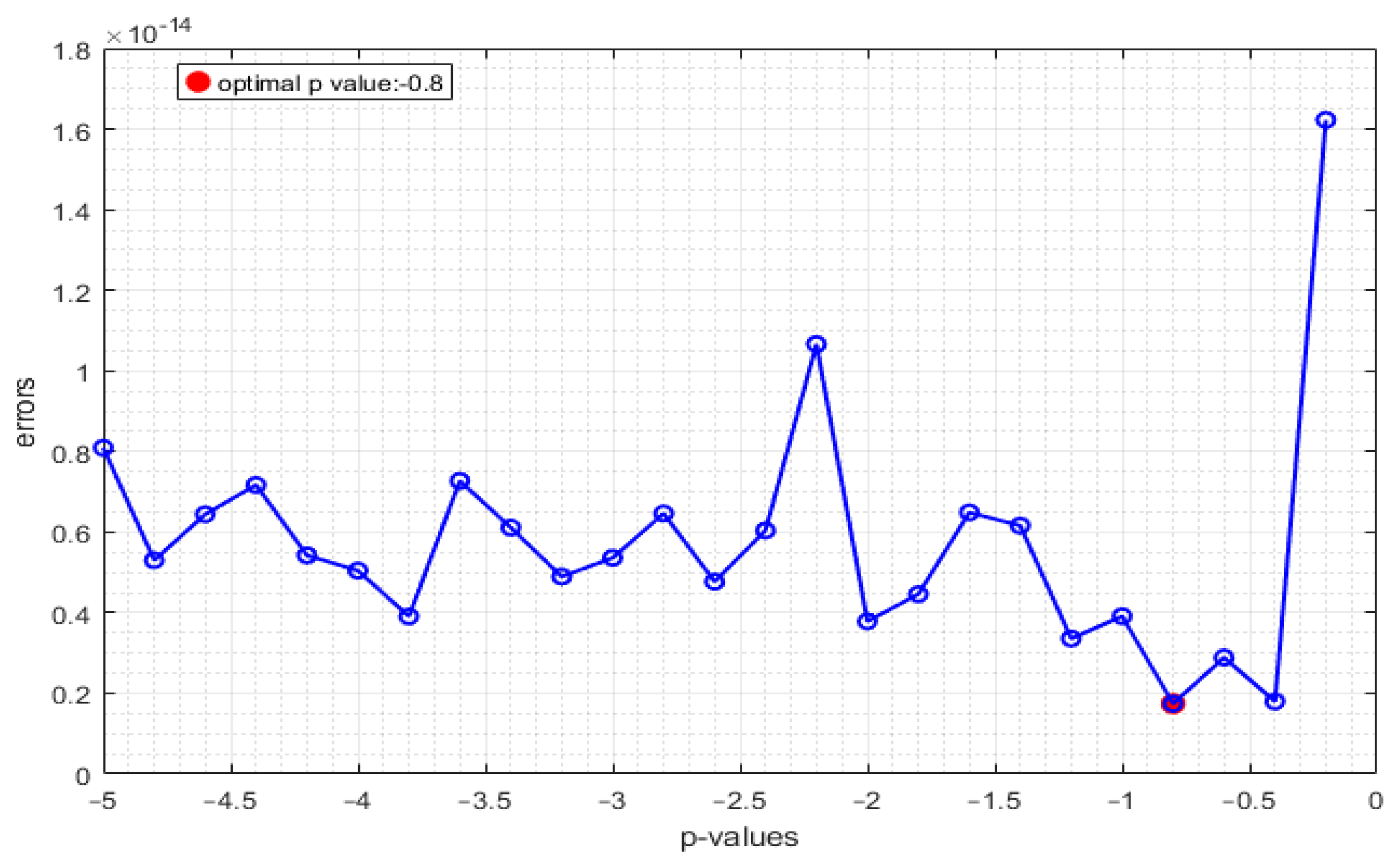
In the example above, the obtained minimum error value is 5.3613 × ${10}^{-15}$ for $p=-3$. However, changing the value of p can further reduce the minimum error. Figure 2 shows the minimum errors corresponding to p-values of the range $-5\le p\le -0.1$ with a step size $0.2$. The graph demonstrates that the minimum error 1.2057 × ${10}^{-15}$ obtained for $p=-0.8$ is smaller than the minimum error obtained for $p=-3$.

Figure 2. Minimum errors of least squares solution of the matrix equation $Q_{\left(E\right)}{X}_{\left(E\right)}=P_{\left(E\right)}$ according to p-values.

In conclusion, the value of p in the elliptic quaternion space emerges as a critical hyperparameter that directly affects the solution to a problem addressed in this space. This finding highlights the significant role of selecting the appropriate p-value in solving any problem and emphasizes that it is a key factor in reducing the error rate. Therefore, optimizing the p-value is important in enhancing solution quality and achieving lower error rates.

4. Color Image Processing Using Singular-Value Decomposition of Elliptic Quaternion Matrices

Elliptic quaternions are distinguished by their composition, comprising one real part alongside three imaginary counterparts. Within the realm of color imagery, particularly in the RGB color space framework, each pixel is constituted by three primary color components, namely red, green, and blue. By drawing an analogy from this, it can be postulated that each pixel within a color image can be analogously represented as a purely imaginary elliptic quaternion, wherein the real component is nullified. In such a representational schema, the red, green, and blue color components are analogically mapped to the i, j, and k components of the purely imaginary elliptic quaternions, respectively. By following this premise, it is possible to articulate that a color image, defined by a dimensional matrix of $m\times n$ pixels, can be succinctly expressed through an elliptic quaternion matrix:

$$f_{\left(E\right)}=R_{\left(E\right),i}i+G_{\left(E\right),j}j+B_{\left(E\right),k}k,$$

where the matrices $R_{\left(E\right),i}$, $G_{\left(E\right),j}$, and $B_{\left(E\right),k}\in {\mathbb{R}}^{m\times n}$ represent the red, green, and blue component matrices of a color image, respectively. This representation is visually illustrated in Figure 3 [18].

Figure 3. Elliptic quaternion matrix representation of the color image airplane.png.

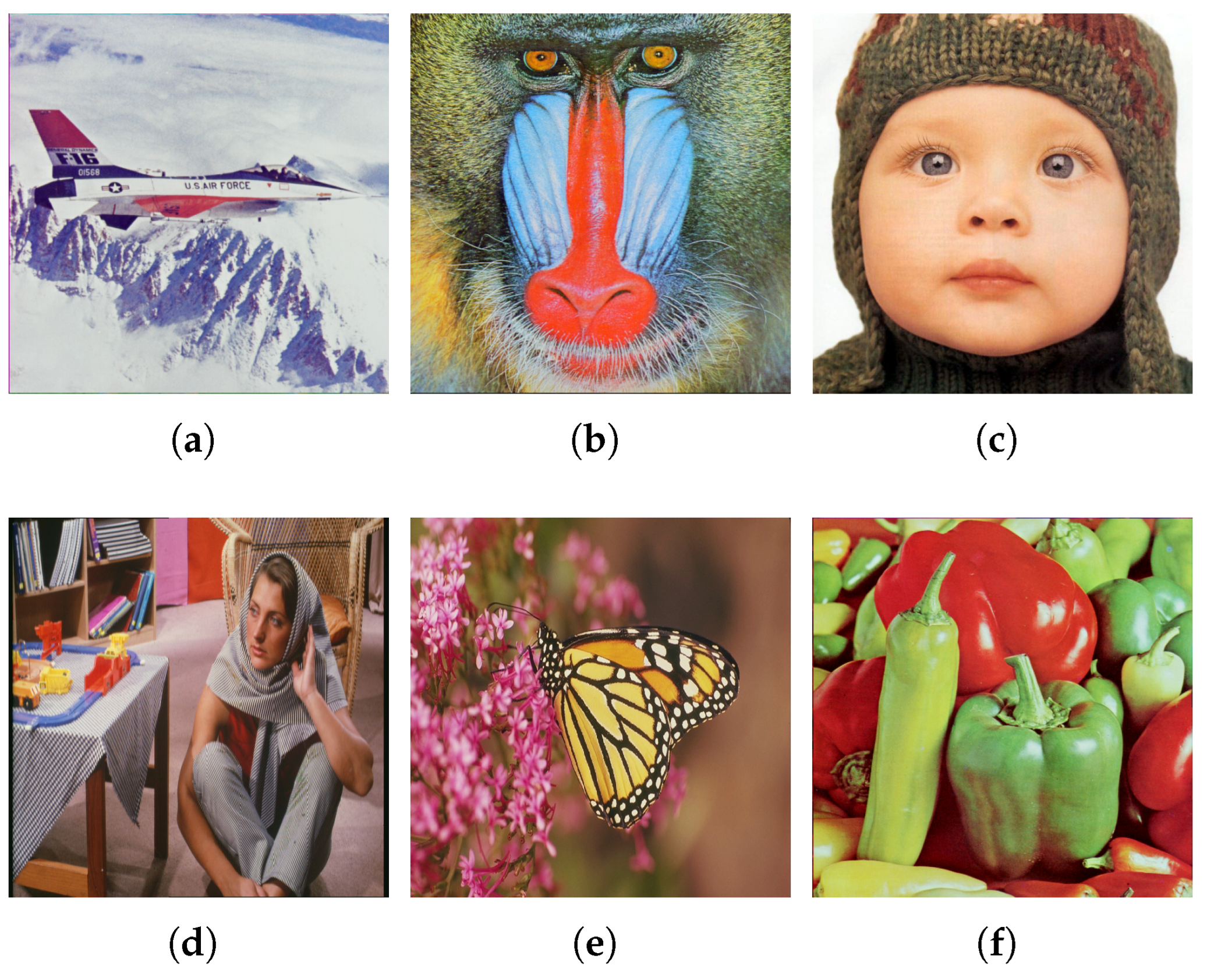
The signatures and descriptions of the image processing functions in the Toolbox are presented in Table 3. The experimental results in this work demonstrate that elliptic quaternion methods outperform other hypercomplex number-based approaches in image analysis and processing (Tables 4–8). The test images used in the experiments of the developed techniques are given in Figure 4. On the other hand, the p-value in the algebra of elliptic quaternions directly affects the performance of the problem modeled in this space (see Figures 11, 13 and 19). As a result, choosing the most appropriate elliptic quaternion space for the problem under consideration (choosing the p-value that gives the most optimal solution to the problem) and the elliptical behavior of many physical systems make this number system more advantageous in image processing. Therefore, incorporating the elliptic quaternion number system into image processing may solve various problems related to time, memory, and performance.

Table 3. Key image processing functions in the toolbox.

Function Name	Description
image2elliptic_q(I,$p$-value)	Returns the elliptic quaternion matrix representation of the image.
	I (Type: uint8, array): The input image in RGB color space
	p-value (Type: negative double)
elliptic_q2image($f_{\left(E\right)}$)	Returns the RGB space representation of an image represented by an elliptical quaternion matrix.
	$f_{\left(E\right)}$ (Type: Object): The elliptic quaternion matrix representation of the image.
elliptic_q_eigenimage($f_{\left(E\right)}$,h)	Returns the desired eigenimages of the image in the elliptic quaternion matrix space.
	h (Type: integer): Specifies the index of the eigenimage to be computed.
elliptic_q_singularvalues($f_{\left(E\right)}$)	It shows the change of singular values of the image in the elliptical quaternion matrix space.
elliptic_q_image_reconstruction($f_{\left(E\right)}$,k)	It compresses the image according to the desired k value in the elliptical quaternion matrix space.
	k (Type: integer): The number of singular values to retain for the reconstruction.
elliptic_q_optimal_p_for_psnr($f_{\left(E\right)}$)	Returns the optimal p (for psnr) value for image compression performed in elliptic quaternion matrix space.
elliptic_q_optimal_p_for_mse($f_{\left(E\right)}$)	Returns the optimal p (for mse) value for image compression performed in elliptic quaternion matrix space.
elliptic_q_embedding_watermarking($f_{\left(E\right)}$,$g_{\left(E\right)}$,alpha)	The embedding_elliptic_watermarking function embeds a watermark into an object using elliptic quaternion matrix algebra.
	$f_{\left(E\right)}$ (Type: Object): The primary object to be watermarked.
	$g_{\left(E\right)}$ (Type: Object): The watermark object to be embedded.
	alpha (Type: Double): The embedding strength parameter.
elliptic_q_extraction_watermarking($f_{\left(E\right)}$,$g_{\left(E\right)}$,U_w,V_w,alpha)	The extraction_elliptic_watermarking function extracts a watermark from a watermarked object using the elliptic quaternion matrix algebra.
	$f_{\left(E\right)}$ (Type: Object): The watermarked object from which the watermark is to be extracted.
	$g_{\left(E\right)}$ (Type: Object): The original, unwatermarked object.
	U_w (Type: Object): The U component of the watermark’s singular-value decomposition.
	V_w (Type: Object): The V component of the watermark’s singular-value decomposition.
elliptic_q_watermarking_optimal_p_for_psnr($f_{\left(E\right)}$,$g_{\left(E\right)}$,alpha)	Finds the optimal p (for psnr) for watermarking using the elliptic quaternion matrix algebra
	$f_{\left(E\right)}$ (Type: Object): The primary object to be watermarked.
	$g_{\left(E\right)}$ (Type: Object): The watermark object to be embedded.
elliptic_q_watermarking_optimal_p_for_mse($f_{\left(E\right)}$,$g_{\left(E\right)}$,alpha)	Finds the optimal p (for mse) for watermarking using the elliptic quaternion matrix algebra.
	$f_{\left(E\right)}$ (Type: Object): The primary object to be watermarked.
	$g_{\left(E\right)}$ (Type: Object): The watermark object to be embedded.

Figure 4. All experimental test images: (a) airplane.png ($512 \times 512$), (b) baboon.png ($512 \times 512$), (c) baby.png ($512 \times 512$), (d) Barbara.png ($576 \times 720$), (e) monarch.png ($512 \times 768$), and (f) peppers.png ($512 \times 512$).

For $p = -0.5$, the elliptic quaternion matrix representation of the test image airplane.png with a resolution of $512 \times 512$ pixels is obtained as in the Listing 5:

Listing 5. MATLAB console output of the function image2elliptic().

On the other hand, a color image can also be represented using elliptic quaternionic singular-value decomposition (ESVD) as

$$f_{\left(E\right)}=U_{\left(E\right)}{\mathsf{\Sigma }}_{\left(E\right)}{V}_{\left(E\right)}^{*},$$

where the matrices $U_{\left(E\right)}$ and $V_{\left(E\right)}$ are unitary matrices and ${\mathsf{\Sigma }}_{\left(E\right)}$ is a hyperbolic matrix. Various image processing techniques can be applied to a color image after applying ESVD without decomposing it into three-channel images. In the subsequent section, principal component analysis, image compression, image restoration, and watermarking techniques were applied to a color image using ESVD.

4.1. Eigenimages of Color Images

The ESVD of any color image can be expressed as

$$f_{\left(E\right)}=U_{\left(E\right)}{\mathsf{\Sigma }}_{\left(E\right)}{V}_{\left(E\right)}^{*}=\sum _{i=1}^R{\sigma }_{i\left(E\right)}\left(u_{i\left(E\right)}\otimes v_{i\left(E\right)}^{*}\right),$$

(1)

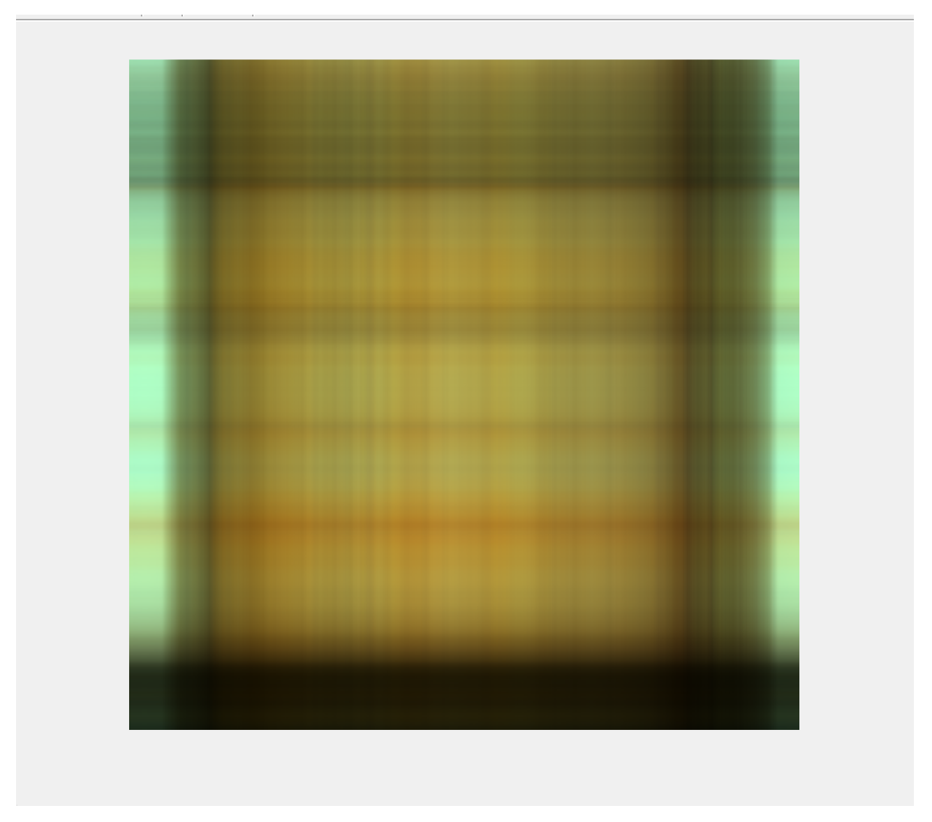
where $u_{i\left(E\right)}\in {\mathbb{H}}_p^{m\times 1}$ and $v_{i\left(E\right)}\in {\mathbb{H}}_p^{n\times 1}$ are elliptic quaternionic vectors, and R represents the rank of the elliptic quaternion matrix $f_{\left(E\right)}$. Each term $u_{i\left(E\right)}\otimes v_{i\left(E\right)}^{*}$ is called an elliptic quaternion-valued eigenimage of the image. Consequently, the color image $f_{\left(E\right)}$ can be thought of as a linear combination of R eigenimages. The first eigenimage, shown in Figure 5, of the test image baby.png is obtained with the function in Listing 6:

Listing 6. MATLAB console output of the functions image2elliptic() and elliptic_q_eigenimage().

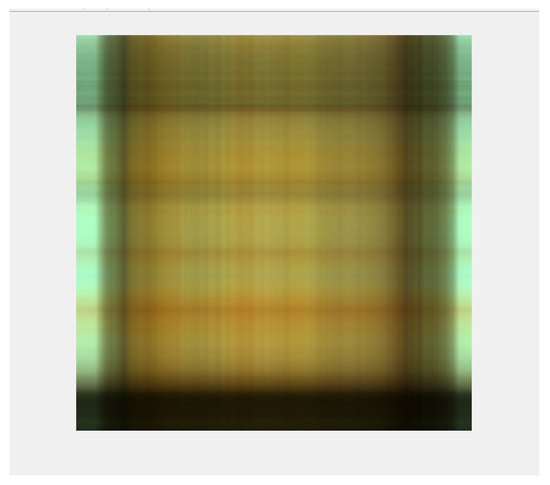
Figure 5. The first eigenimage of the test image baby.png.

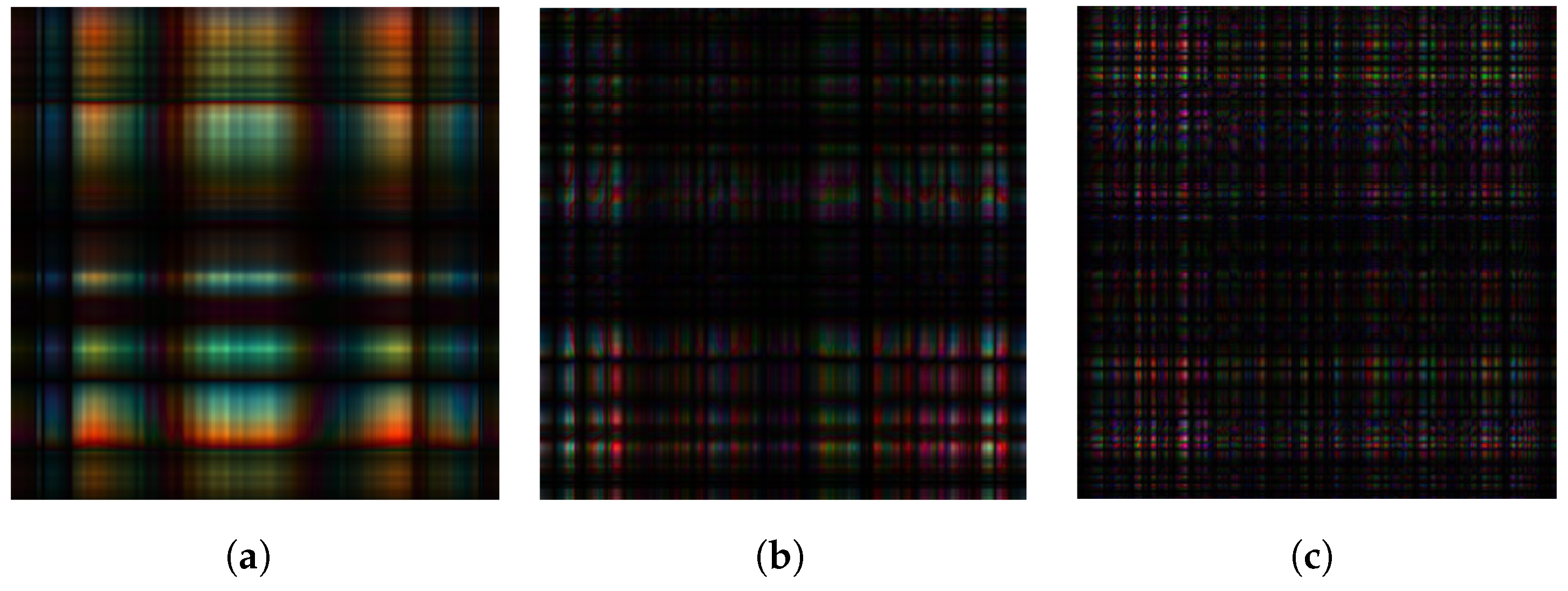
Moreover, normalized absolute versions of the third, tenth, and twenty-fifth eigenimages of the test image baby.png are also given in Figure 6.

Figure 6. Third, tenth, and twenty-fifth eigenimages of the test image baby.png. (a) $u_{3\left(E\right)}\otimes v_{3\left(E\right)}^{*}$. (b) $u_{10\left(E\right)}\otimes v_{10\left(E\right)}^{*}$. (c) $u_{25\left(E\right)}\otimes v_{25\left(E\right)}^{*}$.

As seen in Figure 6, the initial eigenimages correspond to the low-frequency components of the original image, capturing the broad, smooth variations and overall structure. In contrast, the subsequent eigenimages represent the high-frequency components, which detail the finer, more intricate features and textures. This distinction between low- and high-frequency components allows for a more subtle analysis and manipulation of the image data.

4.2. Color Image Compression with ESVD

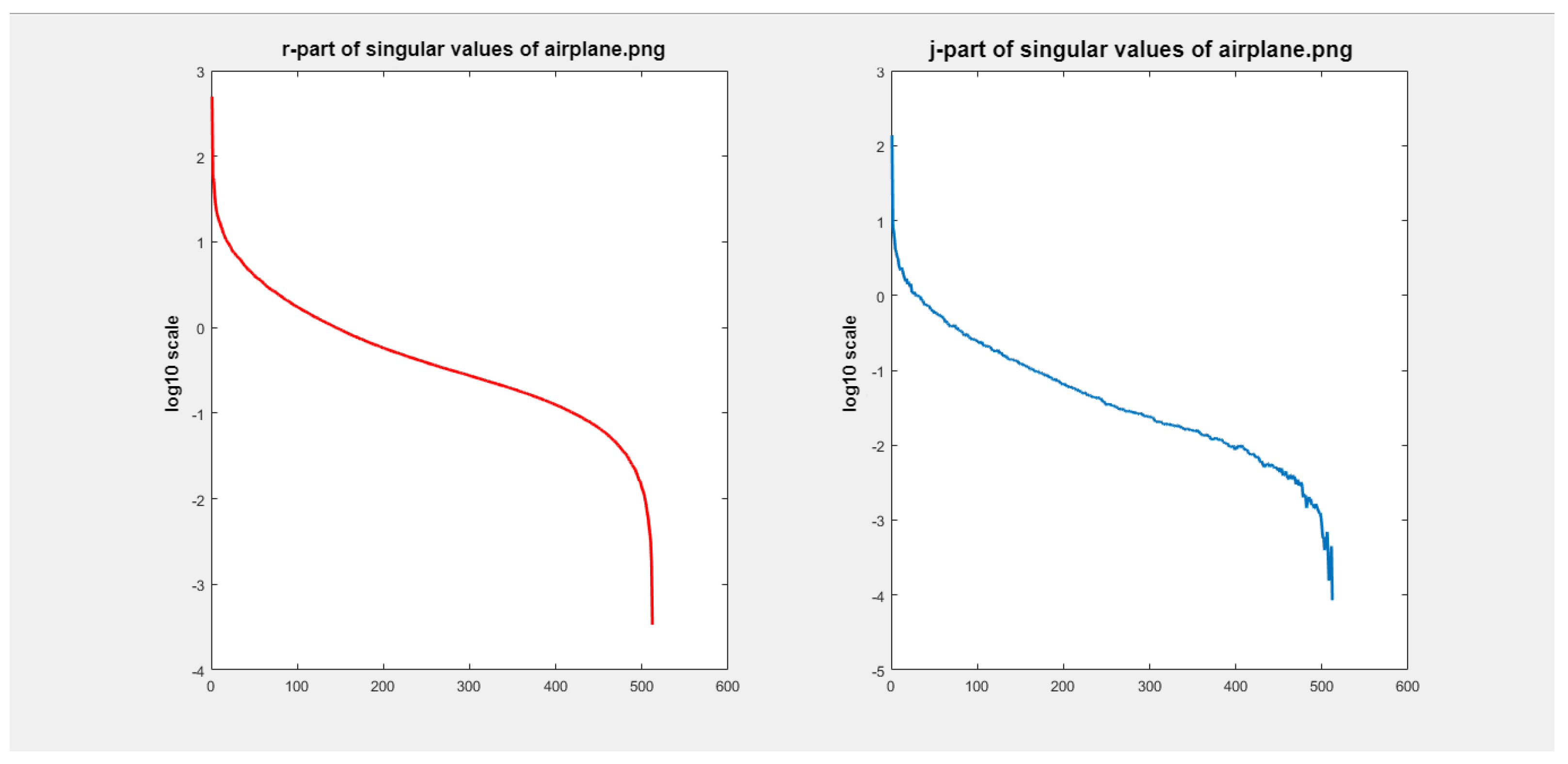
When color images are represented as illustrated in Equation (1), the variation in their singular values can be examined using the function provided in Listing 7. The graph depicted in Figure 7, generated by the function elliptic_q_singularvalues(), demonstrates the variation of the singular values for the test image airplane.png:

Listing 7. MATLAB console output of the functions image2elliptic() and elliptic_q_singularvalues().

Figure 7. Graphs of singular values of the test images airplane.png.

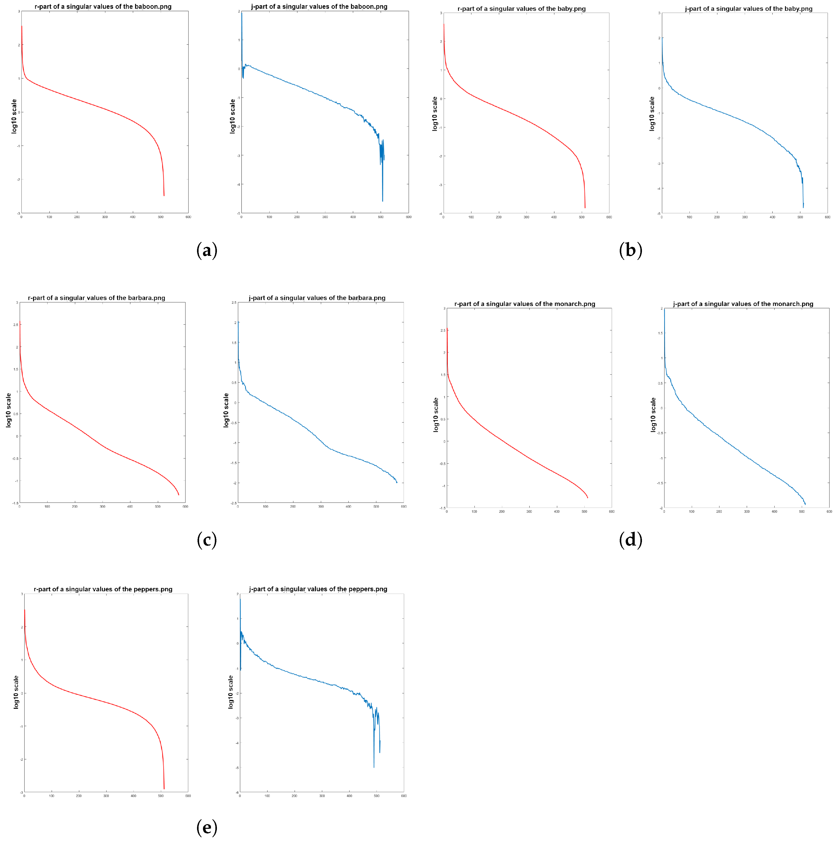
The graphs of singular values of other test images for $p=-0.5$ are shown in Figure 8:

Figure 8. Graphs of singular values of test images: (a) baboon.png, (b) baby.png, (c) Barbara.png, (d) monarch.png, and (e) pepper.png.

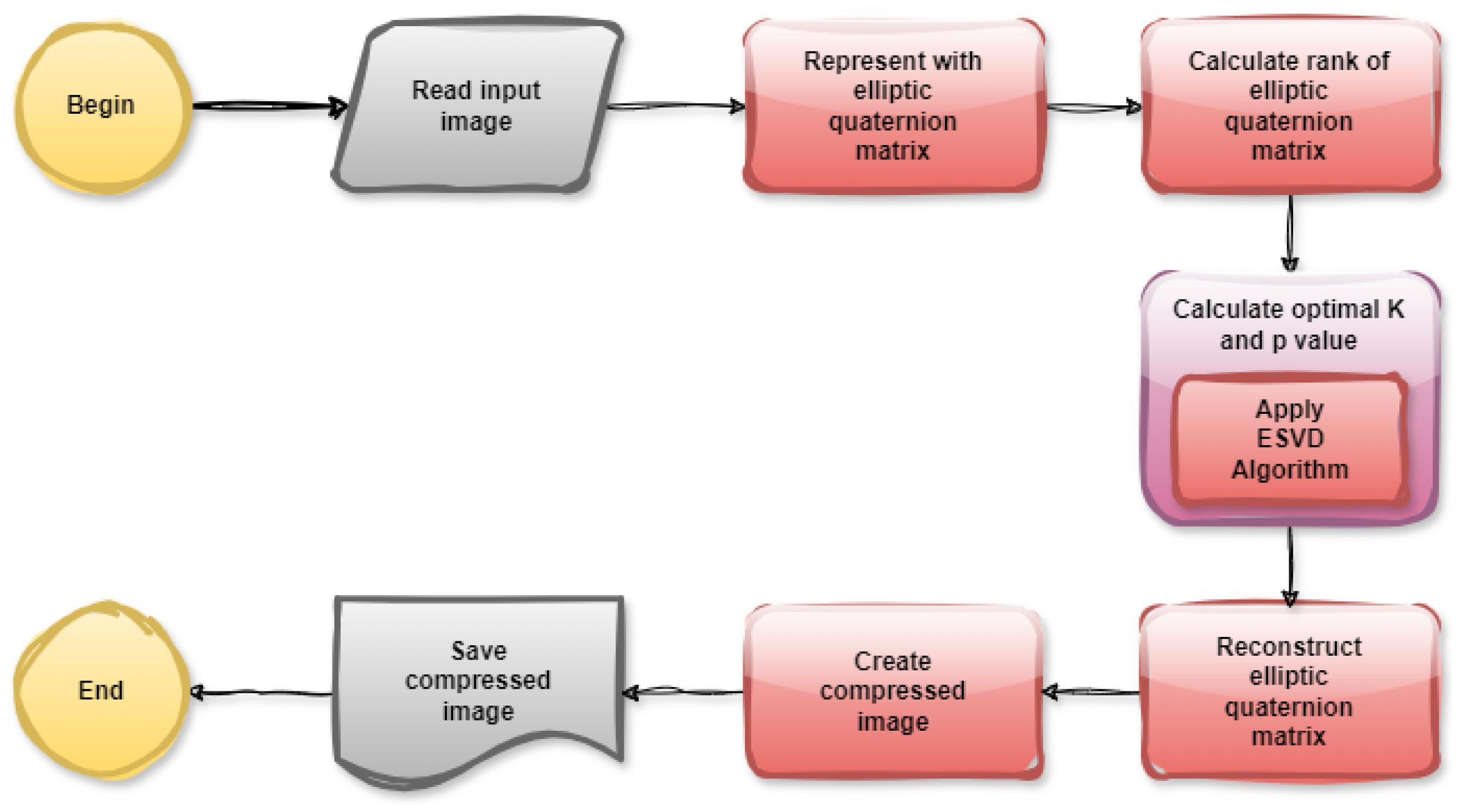
As seen in Figure 7 and Figure 8, the singular values of test images decrease very rapidly. Therefore, even for small values of K satisfying $K<R$, a good approximation of a color image can be achieved. To approximate the matrix $f_{\left(E\right)}$ in Equation (1) for $K<R$, the equation

$$f_{\left(E\right)}=\sum _{i=1}^K{\sigma }_{i\left(E\right)}\left(u_{i\left(E\right)}\otimes v_{i\left(E\right)}^{*}\right)$$

can be used. In this case, the storage space required to store a color image reduces from $3mn$ to $K(m+n+2)$. The steps for image compression with ESVD are provided in Figure 9:

Figure 9. Flowchart of image compression using ESVD.

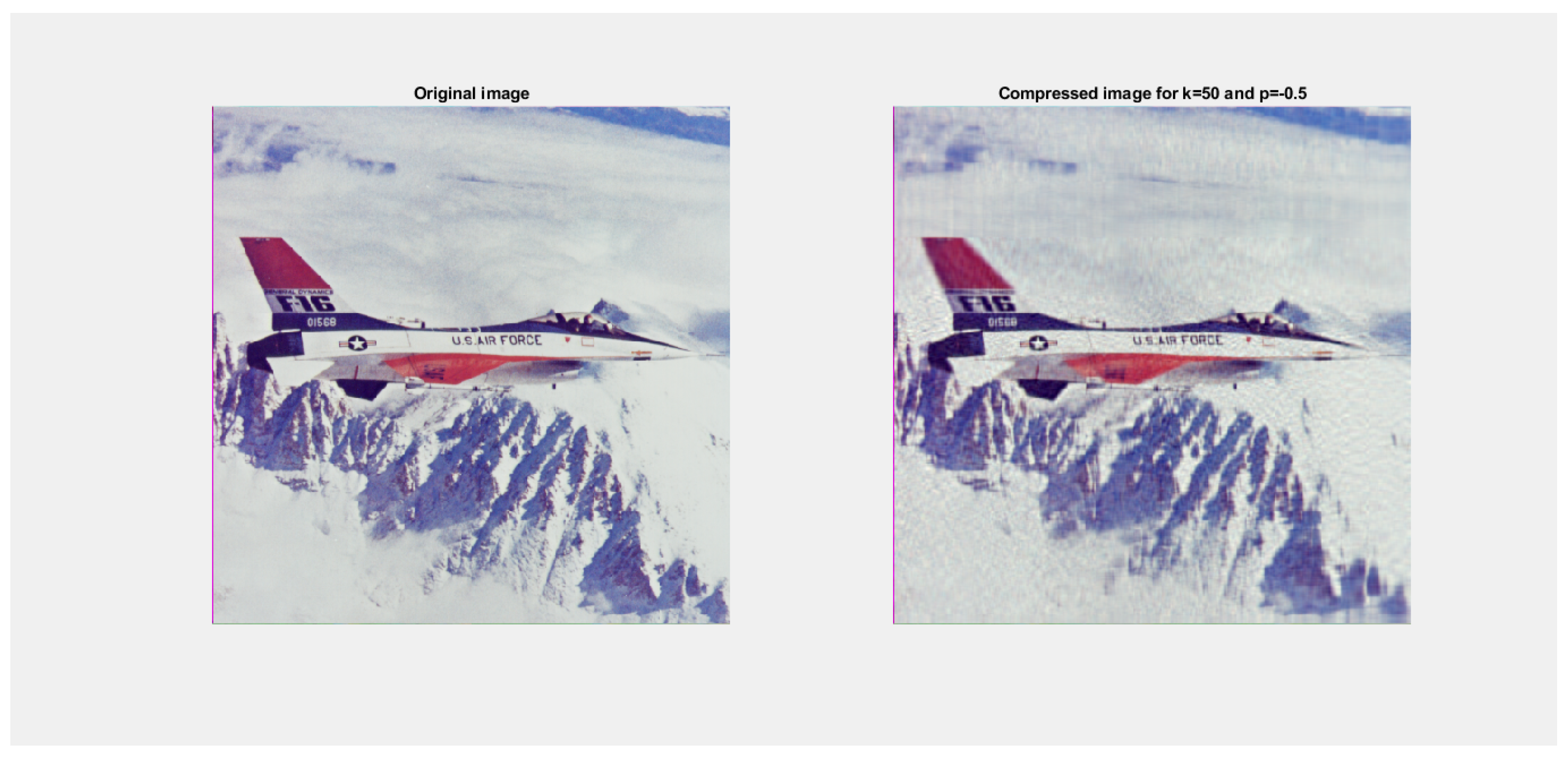
The function in Listing 8 reconstructs the test image airplane.png for $p=-0.5$ and $K=50$. Figure 10 shows the original image airplane.png and the compressed version side-by-side.

Listing 8. MATLAB console output of the function elliptic_q_image_reconstruction().

Figure 10. PSNR and MSE results of the reconstruction of the test image airplane.png for $p = -0.5$ and $K = 50$: PSNR = 30.4527; MSE = 9.0100 × ${10}^{-4}$.

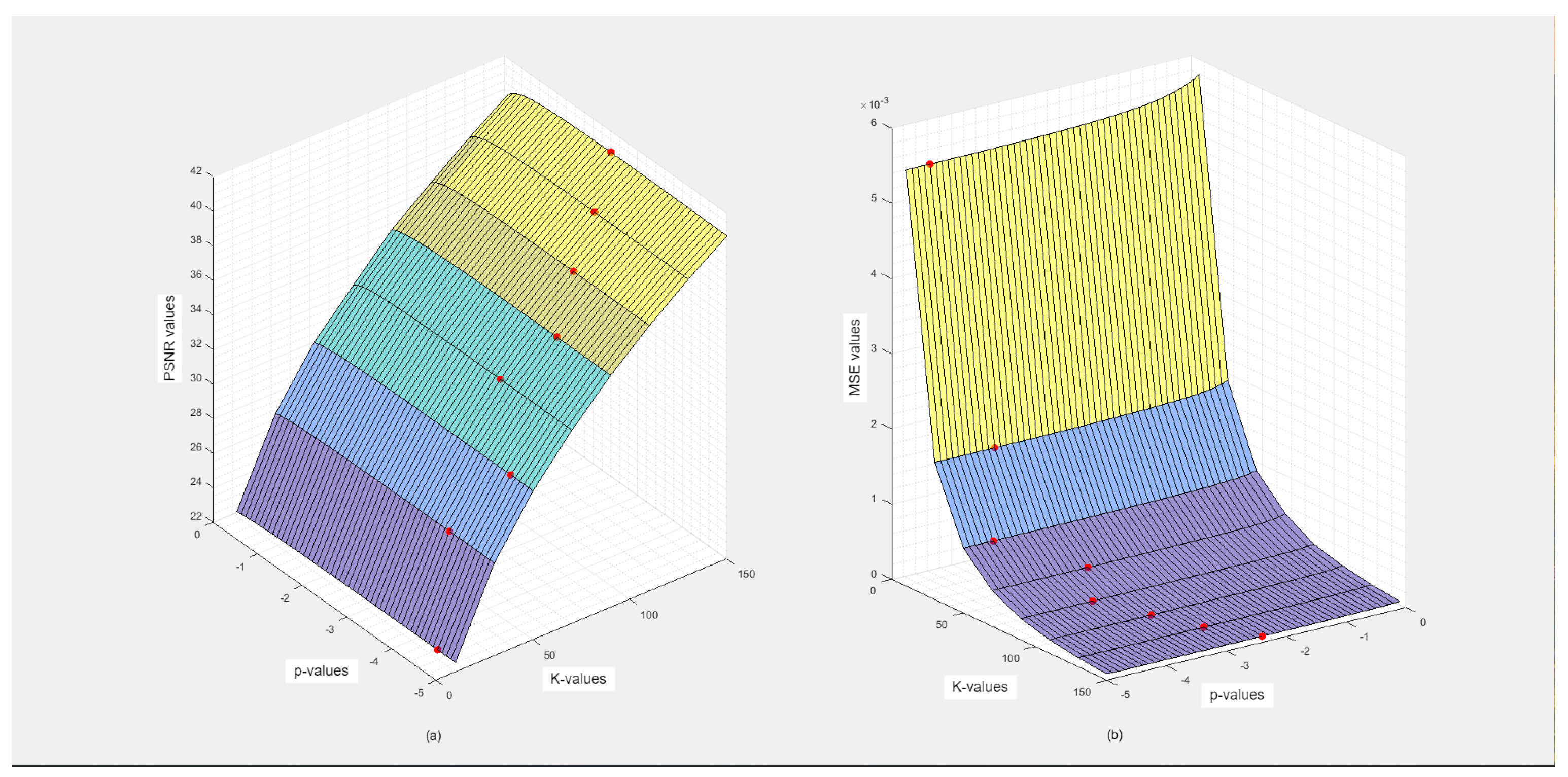
The functions in Listing 9 draw surfaces, which are represented in Figure 11, showing the PSNR (peak signal-to-noise ratio) and MSE (mean squared error) values corresponding to each K and p-value of the test image airplane.png for $K=10:20:150$ and $p=-5:0.1:-0.1$. The red dots indicate optimal p-values.

Listing 9. MATLAB console output of the functions elliptic_q_optimal_p_for_psnr() and optimal_p_for_mse().

Figure 11. Optimal p-values for PSNR and MSE for the test image aiplane.png.

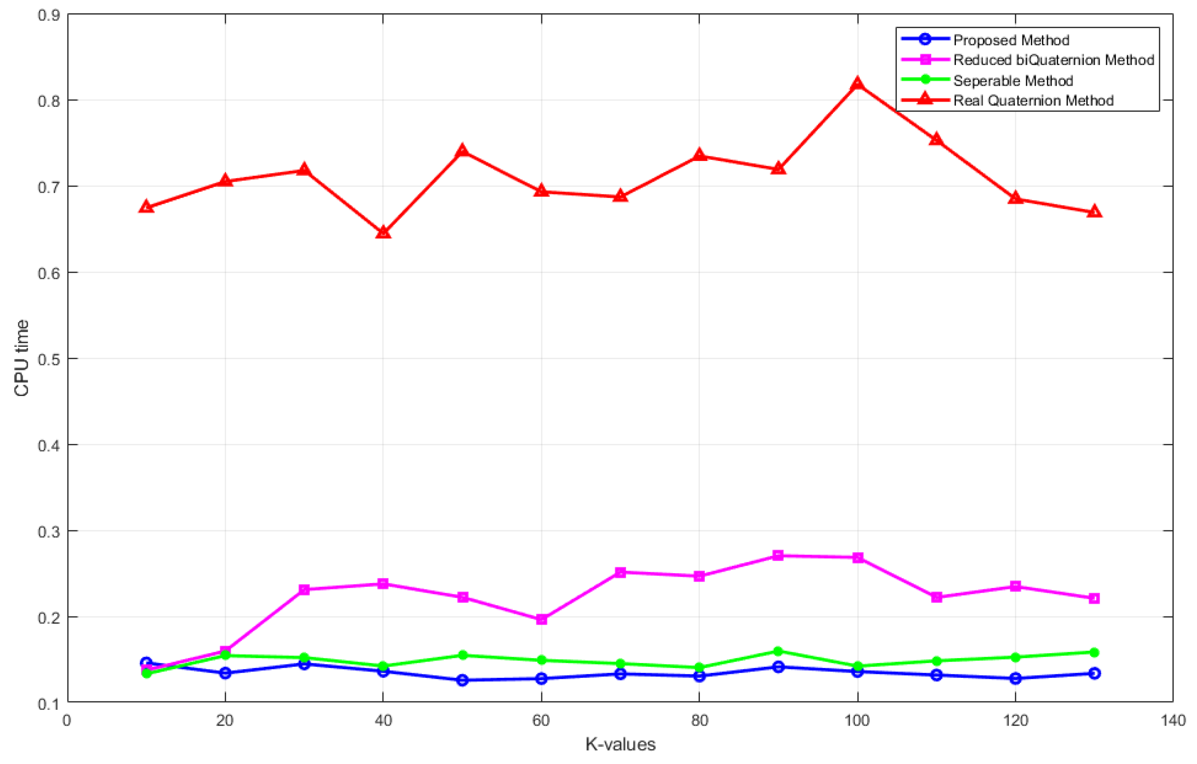
The run time comparison of the proposed ESVD compression method along with the Separable method (compression method obtained by applying singular-value decomposition separately to R, G, and B components) and hypercomplex-based compression methods, such as QSVD (performs singular-value decomposition on real quaternion matrices [21]) and RBSVD (performs singular-value decomposition on reduced biquaternion matrices [22]), on the test images are provided in Figure 12.

Figure 12. Run time comparison of the methods: Separable, QSVD, RBSVD, and ESVD (proposed method) on the test image airplane.png.

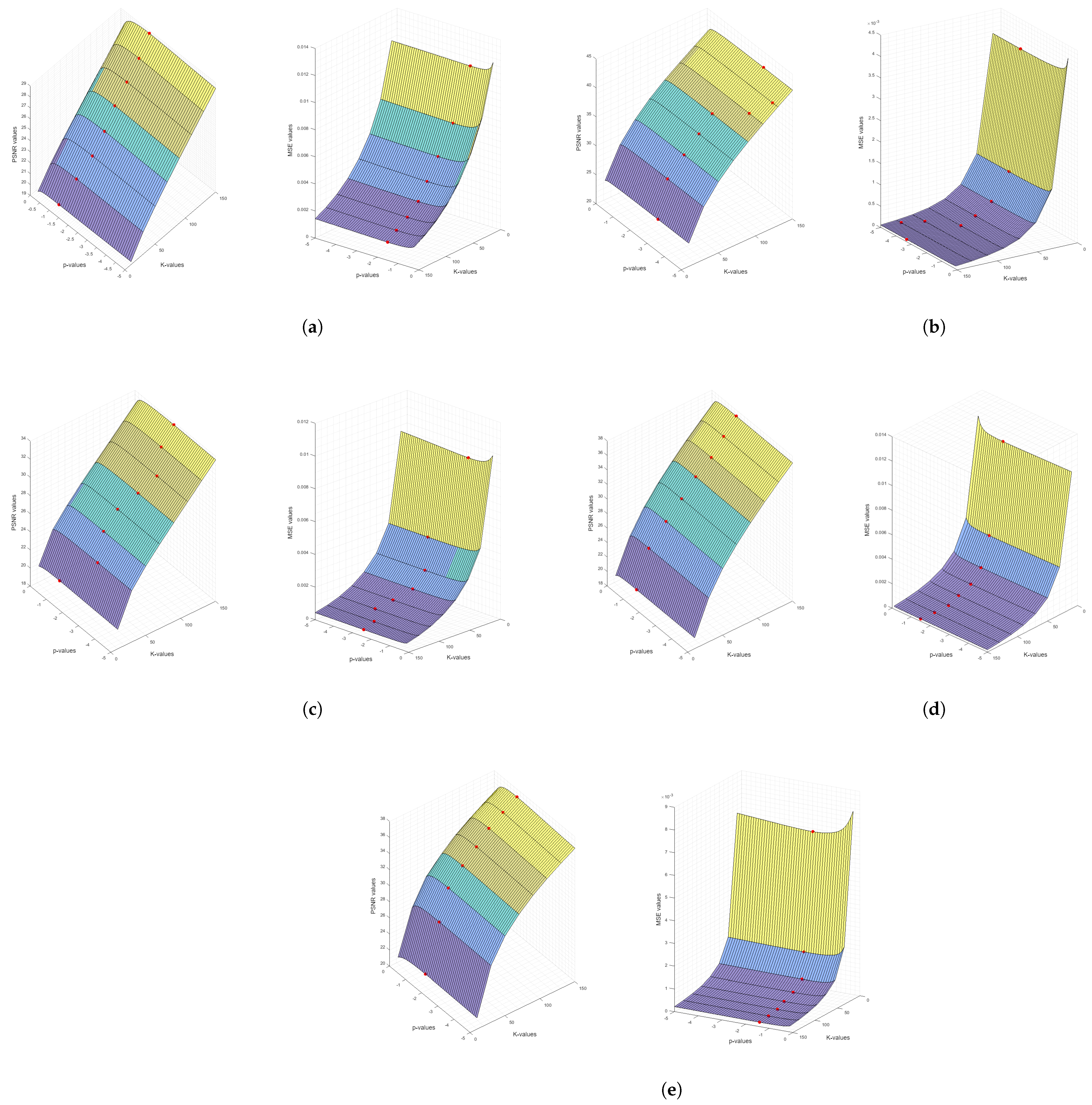
The PSNR and MSE values of all other test images according to the given K and p-values are given in Figure 13.

Figure 13. Optimal p-values for the PSNR and MSE values of the test images: (a) baboon.png, (b) baby.png, (c) Barbara.png, (d) monarch.png, and (e) pepper.png.

The PSNR and MSE values of the proposed ESVD compression method, along with the Separable method and hypercomplex-based compression methods, such as QSVD and RBSVD, on the test images are provided in Table 4 and Table 5.

Table 4. Compression results (PSNR) of Separable, QSVD, RBSVD, and ESVD (proposed method) methods on the test images.

Methods	K	airplane.png	baboon.png	baby.png	Barbara.png	monarch.png	peppers.png
Seperable	10	22.47626	19.22365	23.97807	20.17889	19.47392	21.49341
QSVD	10	22.4593	19.2345	23.9613	20.1977	19.4925	21.4130
RBSVD	10	22.5009	19.3129	24.0043	20.2469	19.561	21.4875
ESVD (Proposed Method)	10	22.5705 ($p=-4.6$)	19.3139 ($p=-1.2$)	24.0406 ($p=-3.2$)	20.2534 ($p=-1.4$)	19.5665 ($p=-1.4$)	21.5484 ($p=-1.8$)
Seperable	50	30.53264	22.36072	32.18642	25.47954	27.17356	29.93859
QSVD	50	30.5012	22.3650	32.2036	25.5249	27.1818	29.9245
RBSVD	50	30.5456	22.504	32.2748	25.6348	27.2814	30.0184
ESVD (Proposed Method)	50	30.6426 ($p=-4.5$)	22.5321 ($p=-1.7$)	32.3295 ($p=-3$)	25.6730 ($p=-2.4$)	27.2899 ($p=-1.5$)	30.0510 ($p=-1.5$)
Seperable	90	35.29278	24.87109	36.67848	28.73954	31.59597	33.3296
QSVD	90	35.2712	24.8850	36.7164	28.7752	31.6127	33.3777
RBSVD	90	35.3386	25.0464	36.8034	28.9119	31.7219	33.4616
ESVD (Proposed Method)	90	35.4537 ($p=-3.8$)	25.0826 ($p=-1.7$)	36.8688 ($p=-2.9$)	28.9695 ($p=-2.8$)	31.7322 ($p=-1.6$)	33.4848 ($p=-1.5$)
Seperable	130	38.97289	27.25229	40.30344	31.8519	35.26918	35.70147
QSVD	130	38.9621	27.2877	40.3574	31.8910	35.3170	35.8012
RBSVD	130	39.0576	27.4817	40.4524	32.0467	35.4109	35.891
ESVD (Proposed Method)	130	39.1724 ($p=-2.9$)	27.5193 ($p=-1.6$)	40.5347 ($p=-4.7$)	32.1148 ($p=-2.5$)	35.4245 ($p=-1.6$)	35.9194 ($p=-1.4$)

Table 5. Compression results (MSE) of Separable, QSVD, RBSVD, and ESVD (proposed method) methods on the test images.

Methods	K	airplane.png	baboon.png	baby.png	Barbara.png	monarch.png	peppers.png
Seperable	10	0.00565	0.01196	0.004	0.0096	0.01129	0.00709
QSVD	10	0.0057	0.0119	0.0040	0.0096	0.0112	0.0072
RBSVD	10	0.0056	0.011714	0.004	0.00944	0.0111	0.0071
ESVD (Proposed Method)	10	0.00553 ($p=-4.6$)	0.011711 ($p=-1.2$)	0.00394 ($p=-3.2$)	0.00943 ($p=-1.4$)	0.01104 ($p=-1.4$)	0.00700 ($p=-1.8$)
Seperable	50	0.00088	0.00581	0.0006	0.00283	0.00192	0.00101
QSVD	50	0.00089	0.0058	0.000602	0.0028	0.0019	0.0010
RBSVD	50	0.00088	0.0056	0.00059	0.00273	0.0019	0.00099
ESVD (Proposed Method)	50	0.00086 ($p=-4.5$)	0.0055 ($p=-1.7$)	0.00058 ($p=-3$)	0.00270 ($p=-2.4$)	0.00186 ($p=-1.5$)	0.00098 ($p=-1.5$)
Seperable	90	0.0003	0.00326	0.00021	0.00134	0.00069	0.00046
QSVD	90	0.000297	0.0032	0.000212	0.0013	0.00068	0.000459
RBSVD	90	0.00029	0.00312	0.000208	0.0013	0.000672	0.00045
ESVD (Proposed Method)	90	0.00028 ($p=-3.8$)	0.00310 ($p=-1.7$)	0.000205 ($p=-2.9$)	0.00126 ($p=-2.8$)	0.000671 ($p=-1.6$)	0.00044 ($p=-1.5$)
Seperable	130	0.00013	0.00188	0.00009	0.00065	0.0003	0.0003
QSVD	130	0.000127	0.0019	0.000092	0.00064	0.000293	0.00026
RBSVD	130	0.000124	0.0018	0.00009	0.00062	0.000287	0.000257
ESVD (Proposed Method)	130	0.00012 ($p=-2.9$)	0.0017 ($p=-1.6$)	0.00008 ($p=-4.7$)	0.00061 ($p=-2.5$)	0.000286 ($p=-1.6$)	0.000256 ($p=-1.4$)

4.3. Color Image Restoration with ESVD

Image restoration is a significant concept in the field of image processing. It entails the estimation of a desired, enhanced image from its degraded version. By utilizing prior knowledge of the degradation phenomena, image restoration techniques aim to remove or reduce degradations introduced during image acquisition—such as noise, pixel value errors, out-of-focus blurring, or camera motion blurring. Generally, the degradation process of an image is nonlinear and spatially variant. However, in applied sciences, this process is often considered linear and spatially invariant, allowing it to be examined using the linear shift invariant (LSI) image restoration model [23].

For an LSI system, f is the original image, g is the observed image, H is the point spread function (PSF) of the imaging system, and n is the additional noise; the following matrix-vector formula expresses the process of image degradation: $g=Hf+n$. Image restoration methods attempt to construct an approximation to f from the observation $g=Hf$. The method of least squares estimator minimizes the sum of squared differences between the real observation g and the predicted observation $Hf.$ The function to be minimized can be equivalently written as ${\Vert g-Hf\Vert }^2$ in matrix-vector notation [23].

Since the color image can be represented by the elliptic quaternion matrix, the image restoration problem is transformed into the elliptic least squares problem of the elliptic quaternion matrix equation $g_{\left(E\right)}=H_{\left(E\right)}{f}_{\left(E\right)}$. As a result, this subsection will present an image restoration model, referred to as ESVD-LSI, based on the singular-value decomposition theory of elliptic quaternion matrices.

In our simulation, Gaussian blur PSFs are employed. Gaussian blur is one of the most prevalent types of blurring that degrades images. It depends on two parameters: the kernel size (hsize) and the standard deviation sigma ($\sigma$) of the Gaussian function in MATLAB. The kernel size determines the dimensions of the pixel area considered during the application of the filter, while the sigma value dictates the amount of blurring; higher sigma values produce a more pronounced blurring effect. These parameters are utilized to simulate the effect of an out-of-focus image or to smooth fine details. The simulation steps are as follows:

• Step 1: An experimental test image is acquired for the ESVD-LSI image restoration method.
• Step 2: PSF is selected manually.
• Step 3: The range of p and step size are selected.
• Step 4: A degraded image is obtained.

In the backend coding, we denote the image matrix of the input image as f. In this case, the elliptic quaternion matrix representation matrix of f is $f_{\left(E\right)}=R_{\left(E\right),i}i+G_{\left(E\right),j}j+B_{\left(E\right),k}k$. The image matrix $R_{\left(E\right),i}$ was degraded with the 2-D Gaussian blur (hsize = 15, $\sigma$ = 1) PSF H to obtain the degraded image matrix $R_{\left(E\right),i}^{\prime }.$ Let $H_{\left(E\right)}=R_{\left(E\right),i}^{\prime }{\left(R_{\left(E\right),i}\right)}^{†}$. In this case, with the help of $H_{\left(E\right)}$, we obtain the elliptic quaternion representation of the degraded image in the form of $g_{\left(E\right)}=H_{\left(E\right)}{f}_{\left(E\right)}$.

• Step 5: According to Theorem 3, the least squares solution with the minimum norm of the elliptic quaternion matrix equation $H_{\left(E\right)}{f}_{\left(E\right)}=g_{\left(E\right)}$ is

$$f_{\left(E\right)}^{\prime }=H_{\left(E\right)}^{†}{g}_{\left(E\right)}=V_{\left(E\right)}{\mathsf{\Sigma }}_{\left(E\right)}^{†}{U}_{\left(E\right)}^{*}{Q}_{2,\left(E\right)},$$

where $H_{\left(E\right)}=U_{\left(E\right)}{\mathsf{\Sigma }}_{\left(E\right)}{V}_{\left(E\right)}^{*}$.

• Step 6: By using the step size and the range of p, the optimal p-value is obtained.
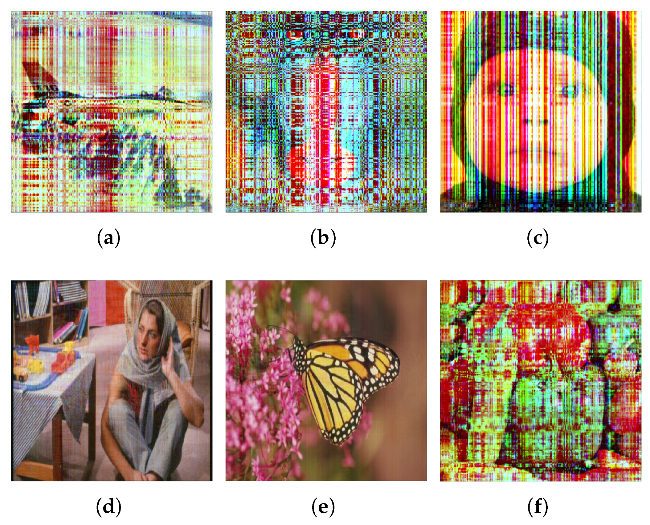
• Step 7: Finally, the enhanced image is obtained by reverse sampling from the elliptic quaternion matrices, which will be obtained by choosing the optimal p-value that makes the least squares error the smallest for ${\Vert g_{\left(E\right)}-H_{\left(E\right)}{f}_{\left(E\right)}\Vert }^2$.

For the results of the simulation system, the test images are degraded according to the instructions in Step 4 for 2-D Gaussian blur (hsize = 15 and $\sigma$ = 1). The degraded images are shown in Figure 14.

Figure 14. Degraded Images: (a) airplane.png, (b) baboon.png, (c) baby.png, (d) Barbara.png, (e) monarch.png, and (f) peppers.png.

After steps 5, 6, and 7, the restored test images according to optimal p-values are given in Figure 15.

Figure 15. Restored images: (a) airplane.png, (b) baboon.png, (c) baby.png, (d) Barbara.png, (e) monarch.png, and (f) peppers.png.

The least squares errors of the QSVD-LSI and RBSVD-LSI restoration methods using the ESVD-LSI restoration method on the test images are provided in Table 6.

Table 6. Comparison of the least squares errors of QSVD-LSI, RBSVD-LSI, and ESVD-LSI (proposed method) on test images.

Methods	airplane.png	baboon.png	baby.png	Barbara.png	monarch.png	peppers.png
QSVD-LSI	$4.1089 \times {10}^{-8}$	$5.6875 \times {10}^{-8}$	$8.9857 \times {10}^{-6}$	$5.5693 \times {10}^{-10}$	$1.7255 \times {10}^{-10}$	$1.1666 \times {10}^{-8}$
RBSVD-LSI	$4.1351 \times {10}^{-8}$	$4.4554 \times {10}^{-8}$	$8.6843 \times {10}^{-6}$	$6.6432 \times {10}^{-10}$	$1.4722 \times {10}^{-10}$	$8.7254 \times {10}^{-9}$
ESVD-LSI (Proposed Method)	$2.9479 \times {10}^{-8}$	$2.9227 \times {10}^{-8}$	$5.6462 \times {10}^{-6}$	$4.0293 \times {10}^{-16}$	$8.3596 \times {10}^{-11}$	$6.2201 \times {10}^{-9}$

4.4. Color Image Watermarking with ESVD

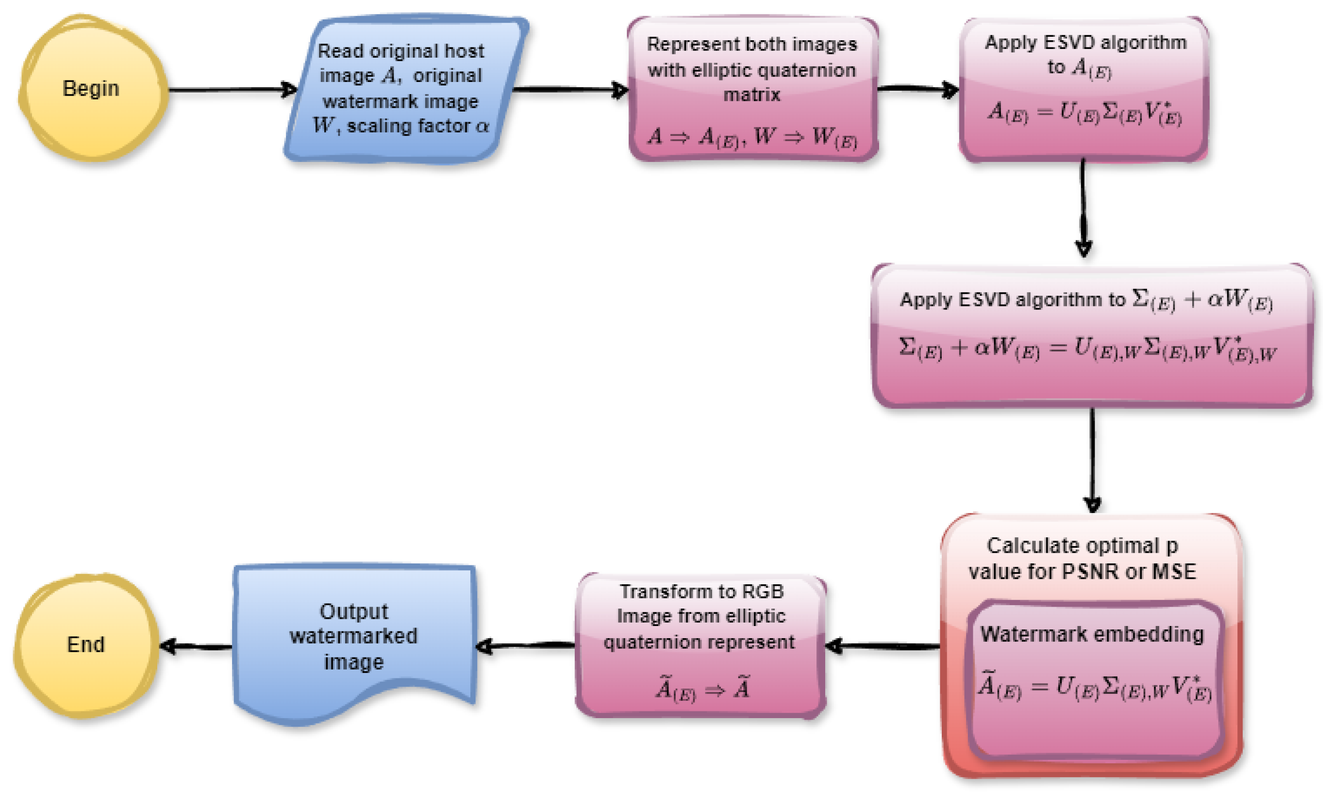
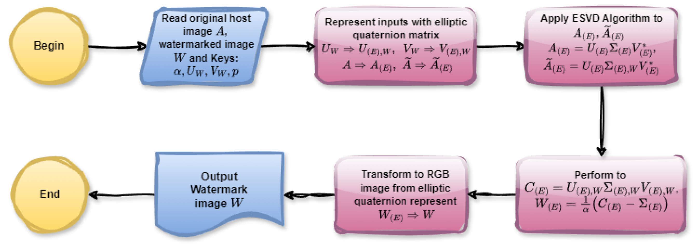
Watermarking is a crucial technique in the field of digital image processing, used extensively for copyright protection, authentication, and data integrity verification. By embedding a watermark into a digital image, one can ensure the traceability and rightful ownership of the content. This technique finds applications in various domains, including media, healthcare, and secure communications. According to the algorithm in [24], we can give a similar algorithm for color image watermarking by using elliptic quaternion matrix algebra. The flowcharts in Figure 16 and Figure 17 illustrate the elliptical quaternion matrix-based color image watermark embedding and extraction procedures, respectively.

Figure 16. The flowchart of watermark embedding.

Figure 17. The flowchart of watermark extracting.

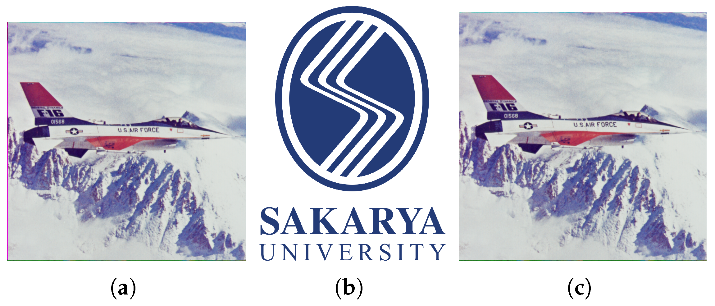
The watermark image sau.png in Figure 18b is embedded in the host image airplane.png via the function elliptic_q_embedding_watermarking() as represented in Listing 10

Listing 10. MATLAB console output of the functions image2elliptic() and elliptic_q_embedding_watermarking().

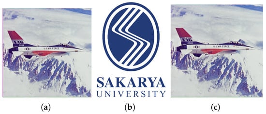
Figure 18. (a) Host image; (b) watermark image; (c) watermarked image.

With the parameters $p=-0.5$ and $\alpha =0.05$. The watermarked image is as in Figure 18c. The PSNR and MSE values between the host and the watermarked images are $59.4340$ and $1.1392\times {10}^{-6}$, respectively.

Figure 19 shows the MSE and PSNR values between the host image and a watermarked image corresponding to p-values given in the range of $-1\le p\le -0.001$ with a step size of $0.001$ ($\alpha =0.05$). According to the graphs, the least MSE is $7.03352\times {10}^{-7}$, and the maximum PSNR is $61.5283$ for the optimal $p=-0.059$.

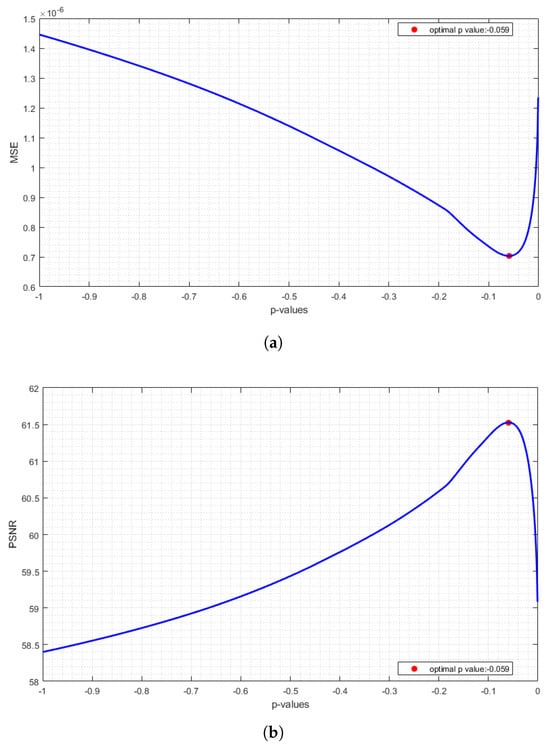
Figure 19. Change in the MSE (a) and PSNR (b) values between the host image and a watermarked image according to p-values.

A comparison of the watermarking methods based on Separable, QSVD, RBSVD, and ESVD in terms of PSNR and MSE on test images are given in Table 7 and Table 8. The proposed method demonstrates better performance than the other approaches.

Table 7. PSNR comparison for the watermarking methods based on Separable, QSVD, RBSVD, and ESVD on the test images.

Methods	$\mathit{\alpha }$	airplane.png	baboon.png	baby.png	Barbara.png	monarch.png	peppers.png
Seperable	0.05	56.9556	62.3572	56.5094	59.5572	58.6407	57.7683
QSVD	0.05	58.3759	65.2280	57.4869	60.8656	59.3973	59.7142
RBSVD	0.05	58.3989	64.8821	57.3881	60.6836	59.2756	59.7100
ESVD (Proposed Method)	0.05	61.5283 optimal $p=-0.059$	66.2703 optimal $p=-0.199$	58.9558 optimal $p=-0.075$	61.5525 optimal $p=-0.093$	60.9556 optimal $p=-0.099$	61.8606 optimal $p=-0.116$

Table 8. MSE comparison for the watermarking methods based on Separable, QSVD, RBSVD, and ESVD on the test images.

Methods	$\mathit{\alpha }$	airplane.png	baboon.png	baby.png	Barbara.png	monarch.png	peppers.png
Separable	0.05	$2.0158 \times {10}^{-6}$	$5.8114 \times {10}^{-7}$	$2.2339 \times {10}^{-6}$	$1.1073 \times {10}^{-6}$	$1.3675 \times {10}^{-6}$	$1.6717 \times {10}^{-6}$
QSVD	0.05	$1.4534 \times {10}^{-6}$	$3.0005 \times {10}^{-7}$	$1.7836 \times {10}^{-6}$	$8.1929 \times {10}^{-7}$	$1.1488 \times {10}^{-6}$	$1.0680 \times {10}^{-6}$
RBSVD	0.05	$1.4458 \times {10}^{-6}$	$3.2493 \times {10}^{-7}$	$1.8247 \times {10}^{-6}$	$8.5435 \times {10}^{-7}$	$1.1815 \times {10}^{-6}$	$1.0691 \times {10}^{-6}$
ESVD (Proposed Method)	0.05	$7.0335 \times {10}^{-7}$ optimal $p=-0.059$	$2.3603 \times {10}^{-7}$ optimal $p=-0.199$	$1.2718 \times {10}^{-6}$ optimal $p=-0.075$	$6.9945 \times {10}^{-7}$ optimal $p=-0.093$	$8.0249 \times {10}^{-7}$ optimal $p=-0.099$	$6.5154 \times {10}^{-7}$ optimal $p=-0.116$

To evaluate the robustness of the proposed watermarking scheme, several attacks, including adding 2% Gaussian noise, cropping one-fourth of the upper-left area of the watermarked image, sharpening, and their sequential application, were performed. The robustness of the watermarking scheme was evaluated using the MSE between the extracted and original watermarks. Table 9 shows the results of the watermarked images for the test images after different attacks. From Table 9, it can be seen that the MSE error values are very small. This result demonstrates the robustness of the proposed scheme against attacks. The watermarks shown in Figure 20 were obtained from the test image airplane.png as a result of the attacks we considered.

Table 9. Results of the MSE of the extracted watermark after different attacks.

Test Images	$\mathit{\alpha }$	Noise 2% Gaussian	Cropping 25%	Noise + Cropping	Sharpening	Noise + Sharpening	Noise + Cropping + Sharpening
airplane.png	0.5	0.0142	0.0010	0.0086	0.0007	0.0396	0.0250
baby.png	0.5	0.0027	0.0017	0.0022	0.0018	0.0123	0.0071
baboon.png	0.5	0.0167	0.0005	0.0099	0.0006	0.0448	0.0281
Barbara.png	0.5	0.0104	0.0015	0.0072	0.0015	0.0313	0.0202
monarch.png	0.5	0.0131	0.0010	0.0077	0.0009	0.0354	0.0214
peppers.png	0.5	0.0088	0.0017	0.0066	0.0005	0.0256	0.0174

Figure 20. The extracted watermarks from the test image airplane.png: (a) Noise, (b) Cropping, (c) Noise + Cropping, (d) Sharpening, (e) Noise + Sharpening, and (f) Noise + Cropping + Sharpening.

5. Conclusions

In color image processing, conventional sparse matrix models employed for representing color images often neglect the interdependencies among the three distinct color channels RGB. Consequently, in numerous image processing tasks, these channels are either processed separately, or the image is converted to grayscale. Such an approach can significantly limit the effectiveness of various image processing techniques, particularly those that rely on the complex interactions of color data. In this study, we applied various color image processing techniques—including principal component analysis, image compression, image restoration, and watermarking—directly to color images represented in the elliptic quaternion algebra without decomposing them into separate RGB channels. These methods were integrated into the MATLAB toolbox developed for this purpose. Extensive experiments were conducted on image compression, reconstruction, image restoration, and watermarking. A comparative performance analysis between the proposed method and other hypercomplex-based compression techniques demonstrated that our method outperformed existing approaches. The experiments also revealed that the choice of the p-value in the algebra of elliptic quaternions directly affects the performance of the solution of the problem under consideration. Selecting an optimal p-value for problem-solving, combined with the elliptic characteristics exhibited by many physical systems, renders this number system advantageous in image processing and other applied fields. Therefore, integrating the elliptic quaternions system into the image processing process can effectively address various challenges related to computational time, memory usage, and overall performance in fields such as machine learning, convolutional neural networks, etc.

On the other hand, the optimal p-values for the problems considered were selected via a brute-force approach by searching in a specific range with a certain step size. It was observed that, in certain cases, the optimal p-values clustered at specific points. Investigating the underlying reasons for this clustering, elucidating the relationship between the optimal p-values and the problems discussed, and developing analytical methods for determining the optimal p-values are proposed as subjects for future research in this article.

References

- Hamilton, W.R. On a new species of imaginary quantities, connected with the theory of quaternions. Proc. R. Ir. Acad. 1840, 2, 424–434. [Google Scholar]
- Adler, S. Quaternionic Quantum Mechanics and Quantum Fields; Oxford University Press: New York, NY, USA, 1995. [Google Scholar]
- Mukundan, R. Quaternions. Advanced Methods in Computer Graphics: With Examples in OpenGL; Springer-Verlag London Limited: London, UK, 2012. [Google Scholar]
- Ell, T.A.; Bihan, N.L.; Sangwine, S.J. Quaternion Fourier Transforms for Signal and Image Processing; Wiley: Hoboken, NJ, USA, 2014. [Google Scholar]
- Parcollet, T.; Morchid, M.; Linares, G. A survey of quaternion neural networks. Artif. Intell. Rev. 2020, 53, 2957–2982. [Google Scholar] [CrossRef]
- Sangwine, S.J.; Bihan, N.L. Quaternion Toolbox for Matlab. Available online: http://qtfm.sourceforge.net/ (accessed on 22 August 2024).
- Pei, S.C.; Chang, J.H.; Ding, J.J. Commutative Reduced Biquaternions and Their Fourier Transform for Signal and Image Processing Applications. IEEE Trans. Signal Process 2004, 52, 2012–2031. [Google Scholar] [CrossRef]
- Navarro-Moreno, J.; Fernández-Alcalá, R.M.; Ruiz-Molina, J.C. Proper ARMA Modeling and Forecasting in the Generalized Segre’s Quaternions Domain. Mathematics 2022, 10, 1083. [Google Scholar] [CrossRef]
- Catoni, F.; Cannata, R.; Zampetti, P. An introduction to commutative quaternions. Adv. Appl. Clifford Algebr. 2006, 16, 1–28. [Google Scholar] [CrossRef]
- Catoni, F.; Boccaletti, D.; Cannata, R.; Catoni, V.; Nichelatti, E.; Zampetti, P. The Mathematics of Minkowski Space–Time: With an Introduction to Commutative Hypercomplex Numbers; Birkhäuser: Basel, Switzerland, 2008. [Google Scholar]
- Yaglom, I.M. A Simple Non-Euclidean Geometry and Its Physical Basis; Springer: New York, NY, USA, 1979. [Google Scholar]
- Condurache, D.; Burlacu, A. Dual tensors based solutions for rigid body motion parameterization. Mech. Mach. Theory 2014, 74, 390–412. [Google Scholar] [CrossRef]
- Catoni, F.; Cannata, R.; Zampetti, P. An introduction to constant curvature spaces in the commutative (Segre) quaternion geometry. Adv. Appl. Clifford Algebr. 2006, 16, 85–101. [Google Scholar] [CrossRef]
- Gai, S. Theory of reduced biquaternion sparse representation and its applications. Expert Syst. Appl. 2023, 213, 119245. [Google Scholar] [CrossRef]
- Kosal, H.H.; Kisi, E.; Akyigit, M.; Celik, B. Elliptic Quaternion Matrices: Theory and Algorithms. Axioms 2024, 13, 656. [Google Scholar] [CrossRef]
- Gai, S.; Huang, X. Reduced biquaternion convolutional neural network for color image processing. IEEE Trans. Circuits Syst. Video Technol. 2022, 32, 1061–1075. [Google Scholar] [CrossRef]
- Kobayashi, M. Twin-multistate commutative quaternion Hopfield neural networks. Neurocomputing 2018, 320, 150–156. [Google Scholar] [CrossRef]
- Atali, G.; Kosal, H.H.; Pekyaman, M. A new image restoration model associated with special elliptic quaternionic least-squares solutions based on LabVIEW. J. Comput. Appl. Math. 2023, 425, 115071. [Google Scholar] [CrossRef]
- Harkin, A.A.; Harkin, J.B. Geometry of generalized complex numbers. Math. Mag. 2004, 77, 118–129. [Google Scholar] [CrossRef]
- Tosun, M.; Kösal, H.H. An Algorithm for Solving the Sylvester s-Conjugate Elliptic Quaternion Matrix Equations. In Algorithms as a Basis of Modern Applied Mathematics. Studies in Fuzziness and Soft Computing; Hošková-Mayerová, Š., Flaut, C., Maturo, F., Eds.; Springer: Cham, Switzerland, 2021; Volume 404. [Google Scholar]
- Chang, J.H.; Ding, J.J. Quaternion matrix singular value decomposition and its applications for color image processing. In Proceedings of the 2003 International Conference on Image Processing (Cat. No. 03CH37429), Barcelona, Spain, 14–17 September 2003; Volume 1, p. I-805. [Google Scholar]
- Pei, S.C.; Chang, J.H.; Ding, J.J.; Chen, M.Y. Eigenvalues and singular value decompositions of reduced biquaternion matrices. IEEE Trans. Circuits Syst. I Regul. Pap. 2008, 55, 2673–2685. [Google Scholar]
- Gunturk, B.K. Fundamental of image restoration. In Image Restoration Fundamentals and Advances; Gunturk, B.K., Li, X., Eds.; CRC Press: New York, NY, USA, 2013; pp. 25–61. [Google Scholar]
- Abd El-Samie, F.E. An efficient singular value decomposition algorithm for digital audio watermarking. Int. J. Speech Technol. 2009, 12, 27–45. [Google Scholar] [CrossRef]
Disclaimer/Publisher’s Note: The statements, opinions and data contained in all publications are solely those of the individual author(s) and contributor(s) and not of MDPI and/or the editor(s). MDPI and/or the editor(s) disclaim responsibility for any injury to people or property resulting from any ideas, methods, instructions or products referred to in the content. |
© 2024 by the authors. Licensee MDPI, Basel, Switzerland. This article is an open access article distributed under the terms and conditions of the Creative Commons Attribution (CC BY) license (https://creativecommons.org/licenses/by/4.0/).