Smoothed Weighted Quantile Regression for Censored Data in Survival Analysis

Abstract

In this study, we propose a smoothed weighted quantile regression (SWQR), which combines convolution smoothing with a weighted framework to address the limitations. By smoothing the non-differentiable quantile regression loss function, SWQR can improve computational efficiency and allow for more stable model estimation in complex datasets. We construct an efficient optimization process based on gradient-based algorithms by introducing weight refinement and iterative parameter estimation methods to minimize the smoothed weighted quantile regression loss function. In the simulation studies, we compare the proposed method with two existing methods, including martingale-based quantile regression (MartingaleQR) and weighted quantile regression (WeightedQR). The results emphasize the superior computational efficiency of SWQR, outperforming other methods, particularly WeightedQR, by requiring significantly less runtime, especially in settings with large sample sizes. Additionally, SWQR maintains robust performance, achieving competitive accuracy and handling the challenges of right censoring effectively, particularly at higher quantiles. We further illustrate the proposed method using a real dataset on primary biliary cirrhosis, where it exhibits stable coefficient estimates and robust performance across quantile levels with different censoring rates. These findings highlight the potential of SWQR as a flexible and robust method for analyzing censored data in survival analysis, particularly in scenarios where computational efficiency is a key concern.

1. Introduction

Survival analysis, a statistical method used to study the time until the occurrence of an event of interest, often faces the challenge of censoring, which occurs when the exact survival time is unknown [1]. Censoring arises in many real-world applications, such as medical studies where some patients may leave the study early, or their event of interest (e.g., death) may not have occurred by the study’s conclusion [2]. Right-censoring, where only the lower bound of the survival time is observed, is the most common type. As noted by Shedden et al. [3], right-censoring was present in 46.6% of patients in their lung cancer study due to factors like transfer to other hospitals or death unrelated to lung cancer. Understanding and addressing this phenomenon is critical for accurate survival time modeling, particularly in clinical trials where survival times are frequently subject to censoring [4,5].

Traditional methods, such as the Cox proportional hazards model and the accelerated failure time (AFT) model, have been widely employed to estimate the conditional distribution of survival time [6,7,8]. However, both approaches rely on the homogeneity assumption, which posits that covariates affect only the expected survival time but not its distributional shape. While these models are computationally convenient and have strong asymptotic properties, they offer limited insights because they primarily focus on the conditional mean of survival time [1,9]. In many practical applications, such as drug efficacy trials, it is more relevant to focus on the tail behavior of the survival distribution, for instance, on the longest surviving patients [10,11]. This limitation of traditional models has prompted the introduction of quantile regression into survival analysis, where the objective is to model the conditional quantiles of the survival time distribution rather than just its mean [12]. Quantile regression offers a comprehensive and flexible alternative to traditional survival analysis methods, enabling the evaluation of covariate effects across the entire distribution of survival times while maintaining interpretable results, as comprehensively reviewed by Peng [13].

Quantile regression, developed by Koenker and Bassett Jr. [14], provides a method to estimate the conditional quantiles of a response variable based on covariates. Powell [12] extended this method to censored data, specifically focusing on the right-censoring scenario. In this case, the observed data are a combination of the minimum of the actual survival time and the censoring time. Powell [12]’s approach provided a way to estimate the quantile regression parameters under right-censoring by modifying the original quantile regression loss function. Subsequent research has expanded upon this work, offering alternative perspectives for handling censored data. One such perspective is the weighted quantile regression approach, as proposed by Portnoy [15] and Wang and Wang [16], which introduces weights to handle different types of censored and uncensored observations. Meanwhile, Peng and Huang [17] approached the problem from a martingale perspective, developing an estimating equation that uses a series of quantile levels to approximate the cumulative effect of censoring on the survival time distribution. However, even with these advances, challenges remain, especially when dealing with censored data and high-dimensional settings [15]. Wang et al. [18] introduced a variable selection method for censored quantile regression, addressing the challenge of identifying significant predictors in survival analysis under censoring. Furthermore, Fei et al. [19] proposed a method for high-dimensional censored quantile regression, enabling improved inference in settings where covariates far exceed the sample size. However, another major hurdle is that the traditional quantile regression loss function is non-differentiable, making it difficult to apply gradient-based optimization techniques, which are commonly used in high-dimensional data analysis [14,20]. In response to these challenges, convolution smoothing has emerged as a powerful technique [21,22]. By smoothing the non-differentiable quantile regression loss function, convolution smoothing transforms the optimization problem into a smooth one, allowing for the use of efficient gradient-based methods [20,23,24]. This approach has garnered significant attention in recent years for its ability to handle both computational complexity and non-smooth optimization issues. Fernandes et al. [20] demonstrated the effectiveness of convolution smoothing in quantile regression without censoring, showing that this method could greatly improve convergence rates while maintaining estimation accuracy. Building on this foundation, He et al. [23] and He et al. [24] extended convolution smoothing techniques to high-dimensional data and censored data using martingale-based approaches, significantly enhancing the scalability of quantile regression in survival analysis. Yan et al. [25] further advanced this area by introducing inference techniques for high-dimensional quantile regression, leveraging convolution smoothing and debiasing to enhance estimation accuracy and hypothesis testing.

In this study, we propose a smoothed weighted quantile regression method based on the framework introduced by Portnoy [15]. The primary objective is to develop an approach that efficiently estimates quantile-specific effects in censored survival data by integrating convolution smoothing into a weighted quantile regression framework. This method addresses the non-differentiability of weighted quantile regression loss functions, enabling stable and computationally efficient estimation, particularly for datasets with varying degrees of censoring. By incorporating convolution smoothing into a weighted quantile regression framework, our method not only resolves the optimization challenges posed by non-smooth loss functions but also leverages adaptive weighting to effectively account for censoring mechanisms. One of the key advantages of our method is its ability to balance accuracy and computational feasibility. In contrast to existing techniques, our method offers superior performance in terms of estimation accuracy across a wide range of quantile levels. By introducing convolution smoothing, we ensure that the optimization problem is smooth and differentiable, which facilitates the use of quasi-Newton and other gradient-based algorithms. This leads to faster convergence and more stable estimates, even in complex survival datasets.

The rest of the paper is organized as follows. In Section 2, we present the methodological framework, including the formulation of the smoothed weighted quantile regression. The algorithm and optimization approach are illustrated in Section 3. Section 4.1 describes the simulation study setup and provides a comparative analysis of SWQR against existing methods. The real data application, which demonstrates the practical effectiveness of SWQR in modeling censored survival data, is detailed in Section 4.2. Discussions and conclusions are provided in Section 5.

2. Methodology

In quantile regression, the conditional quantile function of the response variable Y given covariates X is expressed as

$$F_{Y|X}^{-1}\left(\tau \right)=X^{\top }\beta \left(\tau \right),$$

where $\tau \in (0,1)$ is the quantile level, and $\beta \left(\tau \right)$ represents the quantile-specific regression coefficients. Suppose there are n independent individuals, let $Y_i$ and $X_i={(X_{i1},\dots ,X_{ip})}^{\top }$ denote the response variable and $p\times 1$ vector of covariates for ith individual. For uncensored data, given the observations $(y_i,x_i)$ with $i=1,\dots ,n$, the quantile regression coefficients $\beta \left(\tau \right)$ are estimated by minimizing the following objective function

$$\widehat{\beta }\left(\tau \right)=arg\underset{\beta }{min}{\displaystyle \frac{1}{n}}\sum _{i=1}^n{\rho }_{\tau }(y_i-x_i^{\top }\beta ),$$

where ${\rho }_{\tau }\left(u\right)$ is defined as

$${\rho }_{\tau }\left(u\right)=u(\tau -I(u\le 0)),$$

with $I(u\le 0)$ being the indicator function [26]. This approach works well for uncensored data but cannot handle right-censored observations directly.

This study focuses on estimating the parameters of quantile regression models when the response variable is subject to right-censoring, a common issue in survival analysis and biomedical research. However, when censoring occurs, we only observe ${\tilde{y}}_i=min(y_i,C_i)$, where $C_i$ is the censoring time, and ${\delta }_i=I(y_i\le C_i)$ indicates whether the observation is censored. In the presence of right-censoring, the weights are introduced to account for censored observations [15]. To address the censoring, we first partition the quantile range $(0,\tau )$ into segments as follows

$$0<{\tau }_1<{\tau }_2<\cdots <{\tau }_K=\tau ,$$

which divides the quantile levels into K steps. For each quantile level ${\tau }_k$, according to Portnoy [15], the weighted quantile regression estimator is given by

$${\widehat{\beta }}_w\left({\tau }_k\right)=arg\underset{\beta }{min}{\displaystyle \frac{1}{n}}\sum _{i=1}^n{w}_{i,k}{\rho }_{{\tau }_k}({\tilde{y}}_i-x_i^{\top }\beta )+(1-w_{i,k}){\rho }_{{\tau }_k}(y^M-x_i^{\top }\beta ),$$

(1)

where $w_{i,k}$ are weights for censored and uncensored observations, ${\rho }_{{\tau }_k}\left(u\right)$ is the check function for quantile level ${\tau }_k$, and $y^M$ is a large constant. The weights $w_{i,k}$ are computed based on the censoring status    

$$w_{i,k}=\left\{\begin{array}{cc}1,\hfill & {\delta }_i=1\mathrm{or}({\delta }_i=0\mathrm{and}{\tilde{y}}_i>x_i^{\top }{\widehat{\beta }}_w\left({\tau }_{k-1}\right)),\hfill \\ {\displaystyle \frac{{\tau }_k-{\tau }_{l\left(i\right)}}{1-{\tau }_{l\left(i\right)}}},\hfill & {\delta }_i=0\mathrm{and}{\tilde{y}}_i\le x_i^{\top }{\widehat{\beta }}_w\left({\tau }_{k-1}\right),\hfill \end{array}\right.$$

(2)

where ${\tau }_{l\left(i\right)}$ with $l=1,\dots ,k-1$ and $i=1,\dots ,n$ is the smallest quantile level such that $x_i^{\top }{\widehat{\beta }}_w\left({\tau }_l\right)\ge {\tilde{y}}_i$ for ith individual.

The function ${\rho }_{\tau }\left(u\right)$, known as the check function, is non-smooth at $u=0$, which introduces challenges in optimization since gradient-based methods struggle with non-differentiable points. This non-smoothness often leads to slow convergence or difficulty in obtaining precise parameter estimates. To address this challenge, inspired by the work of [20], we introduce convolution smoothing as a solution. This technique involves applying a smoothing kernel to the check function, effectively transforming it into a smooth and differentiable function, which allows us to leverage gradient-based optimization methods more efficiently. By smoothing the original check function of Equation (1), the optimization becomes more stable and converges more rapidly. The loss function of the smoothed quantile regression can then be expressed as

$$\begin{array}{cc}{R}_{ws}=\hfill & {\displaystyle \frac{1}{n}}\sum _{i=1}^n\left\{w_{i,k}{\int }_{-\infty }^{+\infty }{\rho }_{{\tau }_k}\left(u\right)K_h\left(({\tilde{y}}_i-x_i^{\top }\beta )-u\right)du\right.\hfill \\ \hfill & +\left.(1-w_{i,k}){\int }_{-\infty }^{+\infty }{\rho }_{{\tau }_k}\left(u\right)K_h\left((y^M-x_i^{\top }\beta )-u\right)du\right\},\hfill \end{array}$$

(3)

where $K_h\left(u\right)$ is a kernel function with bandwidth h that controls the level of smoothing. The corresponding regression estimator ${\widehat{\beta }}_{ws}\left({\tau }_k\right)$ can be obtained by minimizing the loss function. In this study, we use the Gaussian kernel, defined as

$$K_h\left(u\right)={\displaystyle \frac{1}{h}}K\left({\displaystyle \frac{u}{h}}\right),K\left(u\right)={\displaystyle \frac{1}{\sqrt{2\pi }}}{e}^{-u^2/2}.$$

The bandwidth h controls the degree of smoothing: a smaller h results in minimal smoothing, while a larger h produces greater smoothing.

The convolution process integrates the check function with the kernel, spreading the residuals ${\tilde{y}}_i-x_i^{\top }\beta$ over a range

$${\int }_{-\infty }^{\infty }{\rho }_{{\tau }_k}\left(u\right)K_h\left(({\tilde{y}}_i-x_i^{\top }\beta )-u\right)du.$$

This smoothing ensures that the resulting objective function is continuously differentiable. This approach maintains the essential properties of the quantile regression model while enabling efficient computation of gradients and Hessians, facilitating faster and more reliable convergence during the optimization process. The gradient of the smoothed loss function is computed as

$${\displaystyle \frac{\partial R_{ws}}{\partial \beta }}={\displaystyle \frac{1}{n}}\sum _{i=1}^n\left[w_{i,k}\left({\int }_{-\infty }^{x_i^{\top }\beta -{\tilde{y}}_i}{K}_h\left(u\right)du-{\tau }_k\right)+(1-w_{i,k})\left({\int }_{-\infty }^{x_i^{\top }\beta -y^M}{K}_h\left(u\right)du-{\tau }_k\right)\right]x_i.$$

(4)

Similarly, the Hessian matrix, representing the second-order derivatives of the smoothed loss function, is given by

$${\displaystyle \frac{{\partial }^2{R}_{ws}}{\partial \beta \partial {\beta }^{\top }}}={\displaystyle \frac{1}{n}}\sum _{i=1}^n\left[w_{i,k}{K}_h(x_i^{\top }\beta -{\tilde{y}}_i)+(1-w_{i,k})K_h(x_i^{\top }\beta -y^M)\right]x_i{x}_i^{\top }.$$

(5)

This smoothed approach not only ensures the differentiability of the loss function but also facilitates the computation of gradients and Hessians, which are essential for efficient optimization using quasi-Newton methods or other gradient-based algorithms. This methodology integrates convolution smoothing and weighted quantile regression to efficiently estimate parameters in the presence of right-censored data. By smoothing the check function, the optimization process is made more efficient while retaining the key properties of quantile regression. Translation tools, including Youdao Dictionary software and Google Translate, were used to assist in grammar correction and language refinement during the preparation of this study.

3. Computational Algorithm

In this study, we employ a line search method combined with a quasi-Newton approach [24]. Specifically, we utilize the Barzilai-Borwein (BB) step size method, first introduced by Barzilai and Borwein [27]. This method has been proven to enhance the efficiency of gradient-based algorithms, particularly in large-scale optimization problems. In this context, the gradient $g^{\left(t\right)}$, step direction $d^{\left(t\right)}$, and Hessian approximation $H^{\left(t\right)}$ are computed at each iteration t. We define ${\delta }^{\left(t\right)}={\beta }^{(t+1)}-{\beta }^{\left(t\right)}$, representing the change in the estimated parameters between iterations. Similarly, $g^{\left(t\right)}=d^{\left(t\right)}-d^{(t-1)}$, denotes the difference between successive gradients. The method satisfies the secant Equation ${\delta }^{\left(t\right)}\approx {\eta }^{\left(t\right)}{g}^{\left(t\right)}$, where the scalar ${\eta }^{\left(t\right)}$ is determined by minimizing the following least squares problem

$${\eta }^{\left(t\right)}=arg\underset{\eta }{min}{∥{\delta }^t-\eta g^{\left(t\right)}∥}_2^2.$$

That is, ${\eta }^{\left(t\right)}$ can be calculated as

$${\eta }^{\left(t\right)}={\displaystyle \frac{\langle {\delta }^{\left(t\right)},g^{\left(t\right)}\rangle }{\langle g^{\left(t\right)},g^{\left(t\right)}\rangle }}.$$

The quasi-Newton algorithm (Algorithm 1) with Barzilai-Borwein step size method is as follows.

Algorithm 1: BB-Quasi–Newton Algorithm

To solve the optimization problem presented in Equation (3), we introduce a weight refinement and iterative parameter estimation methods into gradient-based algorithms to minimize the smoothed weighted quantile regression loss function. Compared to traditional linear programming optimization models, this approach significantly improves computational efficiency. The optimization process is based on the above BB-Quasi–Newton algorithm. Assume we have sample observations ${\left\{({\tilde{y}}_i,{\delta }_i,x_i)\right\}}_{i=1}^n$, quantile levels ${\tau }_1<{\tau }_2<\cdots <{\tau }_K$, initial value ${\beta }^{\left(0\right)}$, initial learning rate ${\eta }^{\left(0\right)}$, maximum iterations maxTime and tolerance tol, the optimization process is as follows.

Step 1: 

For the first quantile level ${\tau }_1$, directly set $w_{i,1}^{\mathrm{c}}=1$, substitute into Line 17, and calculate the initial estimate ${\widehat{\beta }}_{ws}^{\mathrm{c}}\left({\tau }_1\right)$.

Step 2: 

Assume we have obtained ${\widehat{\beta }}_{ws}^{\mathrm{c}}\left({\tau }_l\right)$, for $l=1,\dots ,k-1$. For each $i=1,2,\dots ,n$, if $x_i^{\top }{\widehat{\beta }}_{ws}^{\mathrm{c}}\left({\tau }_{k-1}\right)\ge {\tilde{y}}_i$, calculate the temporary quantile level

$${\tau }_{l\left(i\right)}^t={\displaystyle \frac{\left[x_i^{\top }{\widehat{\beta }}_{ws}^{\mathrm{c}}\left({\tau }_{l\left(i\right)}\right)-{\tilde{y}}_i\right]{\tau }_{l\left(i\right)}+\left[{\tilde{y}}_i-x_i^{\top }{\widehat{\beta }}_{ws}^c\left({\tau }_{l\left(i\right)-1}\right)\right]{\tau }_{l\left(i\right)-1}}{x_i^{\top }{\widehat{\beta }}_{ws}^c\left({\tau }_{l\left(i\right)}\right)-x_i^{\top }{\widehat{\beta }}_{ws}^c\left({\tau }_{l\left(i\right)-1}\right)}}.$$

Step 3: 

Use ${\tau }_{l\left(i\right)}^t$ from Step 2, substitute into the following equation, and calculate the temporary weight $w_{i,k}^t$ with $i=1,\dots ,n$,

$$w_{i,k}^t=\left\{\begin{array}{cc}1,\hfill & {\delta }_i=1\mathrm{or}({\delta }_i=0\mathrm{and}{\tilde{y}}_i>x_i^{\top }{\widehat{\beta }}_{ws}^{\mathrm{c}}\left({\tau }_{k-1}\right)),\hfill \\ {\displaystyle \frac{{\tau }_k-{\tau }_{l\left(i\right)}^t}{1-{\tau }_{l\left(i\right)}^t}},\hfill & {\delta }_i=0\mathrm{and}{\tilde{y}}_i\le x_i^{\top }{\widehat{\beta }}_{ws}^{\mathrm{c}}\left({\tau }_{k-1}\right).\hfill \end{array}\right.$$

Step 4: 

Substitute the temporary weight $w_{i,k}^t$ from Step 3 into Equation (3), and apply the BB-Quasi–Newton algorithm to compute ${\widehat{\beta }}_{ws}^t\left({\tau }_k\right)$.

Step 5: 

For observations where $x_i^{\top }{\widehat{\beta }}_{ws}^{\mathrm{c}}\left({\tau }_{k-1}\right)<{\tilde{y}}_i<x_i^{\top }{\widehat{\beta }}_{ws}^t\left({\tau }_k\right)$, recompute ${\tau }_{l\left(i\right)}^{\mathrm{c}}$ using the following formula

$${\tau }_{l\left(i\right)}^{\mathrm{c}}={\displaystyle \frac{(x_i^{\top }{\widehat{\beta }}_{ws}^t\left({\tau }_k\right)-{\tilde{y}}_i){\tau }_k+({\tilde{y}}_i-x_i^{\top }{\widehat{\beta }}_{ws}^c\left({\tau }_{k-1}\right)){\tau }_{k-1}}{x_i^{\top }{\widehat{\beta }}_{ws}^t\left({\tau }_k\right)-x_i^{\top }{\widehat{\beta }}_{ws}^c\left({\tau }_{k-1}\right)}}.$$

Step 6: 

Substitute the results from Steps 5 and 2 into the following equation to recalculate the weight $w_{i,k}^{\mathrm{c}}$,

$$w_{i,k}^{\mathrm{c}}=\left\{\begin{array}{cc}1,\hfill & {\delta }_i=1\mathrm{or}({\delta }_i=0\mathrm{and}{\tilde{y}}_i>x_i^{\top }{\widehat{\beta }}_{ws}^t\left({\tau }_k\right)),\hfill \\ {\displaystyle \frac{{\tau }_k-{\tau }_{l\left(i\right)}^{\mathrm{c}}}{1-{\tau }_{l\left(i\right)}^{\mathrm{c}}}},\hfill & {\delta }_i=0\mathrm{and}{\tilde{y}}_i\le x_i^{\top }{\widehat{\beta }}_{ws}^t\left({\tau }_k\right).\hfill \end{array}\right.$$

Step 7: 

Finally, substitute the updated weight $w_{i,k}^{\mathrm{c}}$ into the following equation and use the BB-Quasi–Newton algorithm to compute the final estimate ${\widehat{\beta }}_{ws}^{\mathrm{c}}\left({\tau }_k\right)$,

$$\begin{array}{c}\hfill {\widehat{\beta }}_{ws}^{\mathrm{c}}\left({\tau }_k\right)=arg\underset{\beta }{min}{\displaystyle \frac{1}{n}}\sum _{i=1}^n\left\{w_{i,k}^{\mathrm{c}}{\int }_{-\infty }^{+\infty }{\rho }_{{\tau }_k}\left(u\right)K_h\left(({\tilde{y}}_i-x_i^{\top }\beta )-u\right)du\right.\\ \hfill +\left.(1-w_{i,k}^{\mathrm{c}}){\int }_{-\infty }^{+\infty }{\rho }_{{\tau }_k}\left(u\right)K_h\left((y^M-x_i^{\top }\beta )-u\right)du\right\}.\end{array}$$

4. Results

4.1. Simulation Study

In this section, we present a detailed simulation study to evaluate the performance of the proposed smoothed weighted quantile regression method for censored data. We compare our approach with two existing methods, including the weighted quantile regression method and martingale-based quantile regression method [15,17]. Portnoy [15] proposed a recursively reweighted estimation procedure for censored quantile regression, extending the Kaplan–Meier estimator to handle more complex regression settings involving censoring. On the other hand, Peng and Huang [17] developed a martingale-based estimating equation, which simplifies quantile regression with survival data by minimizing $\mathrm{L}1$-type convex functions, ensuring computational efficiency and robustness. For the comparison methods, the quantreg package in R is used, employing the crq.fit.por and crq.fit.pen functions for Portnoy [15]’s and Peng and Huang [17]’s methods, respectively. All simulations were executed on a workstation equipped with two 24-core 2.99 GHz CPUs and 128 GB of memory. Each simulation run utilized 8 CPU cores concurrently.

In the simulation study, the covariates $x_i\in {\mathbb{R}}^p$ are split into three groups

$$\begin{array}{c}{x}_i=(x_{i,1},\cdots ,x_{i,p_1},x_{i,p_1+1},\dots ,x_{i,p_2},x_{i,p_2+1},\dots ,x_{i,p}),\hfill \end{array}$$

where the first $p_1$ covariates $x_{i,j}$ with $j=1,\dots ,p_1$ follow a multivariate normal distribution $N(0,\Sigma )$, and the remaining covariates come from a mixture of normal and binomial distributions. Specifically, $x_{i,j}$ with $j=1,\dots ,p_1$ follow a multivariate normal distribution $N(0,\Sigma )$, where $\Sigma$ is a $p_1\times p_1$ covariance matrix with ${\sigma }_{j,k}=0.5^{|j-k|}$, for $1\le j,k\le p_1$. The second group of covariates, $x_{i,j}$ with $j=p_1+1,\dots ,p_2$, follows a multivariate uniform distribution on the interval ${[-2,2]}^{p_2-p_1}$ with covariance matrix $\Sigma$, and the final group $x_{i,j}$ with $j=p_2+1,\dots ,p$ consists of binary variables drawn from a Bernoulli distribution with probability 0.5. The response variable $y_i={\tilde{x}}_i^{\top }\gamma +{ϵ}_i$, where ${\gamma }_j\sim \mathrm{U}(-2,2),j=1,2,\dots ,p$, ${ϵ}_i\sim t_2$. Let $Q_{t_2}\left(\tau \right)$ represent the quantile function of the t-distribution with 2 degrees of freedom and denote $x_i={(1,{\tilde{x}}_i^{\top })}^{\top }$, the response variable $y_i$ is generated according to the following model

$$y_i=x_i^{\top }{\beta }^{*}\left(\tau \right)+({ϵ}_i-Q_{t_2}\left(\tau \right)),$$

where ${\beta }^{★}\left(\tau \right)={\left(Q_{t_2}\left(\tau \right),{\gamma }^{\top }\right)}^{\top }$, $\gamma ={({\gamma }_1,\dots ,{\gamma }_p)}^{\top }$ with ${\gamma }_i$ follows a uniform distribution on interval $[-2,2]$ and ${ϵ}_i$ follows t-distribution with 2 degrees of freedom. Random censoring $C_i$ is introduced by sampling censoring times from a mixture distribution:

$$C_i=I(u_i=1)N(0,16)+I(u_i=2)N(5,1)+I(u_i=3)N(10,0.25),i=1,\dots ,n,$$

where $u_i$ are randomly drawn from the set $\{1,2,3\}$. The observed response ${\tilde{y}}_i$ is then the minimum of the true response and the censoring time, ${\tilde{y}}_i=min(y_i,C_i)$. Furthermore, the bandwidth of the Gaussian kernel for our method is selected as $h=0.035$.

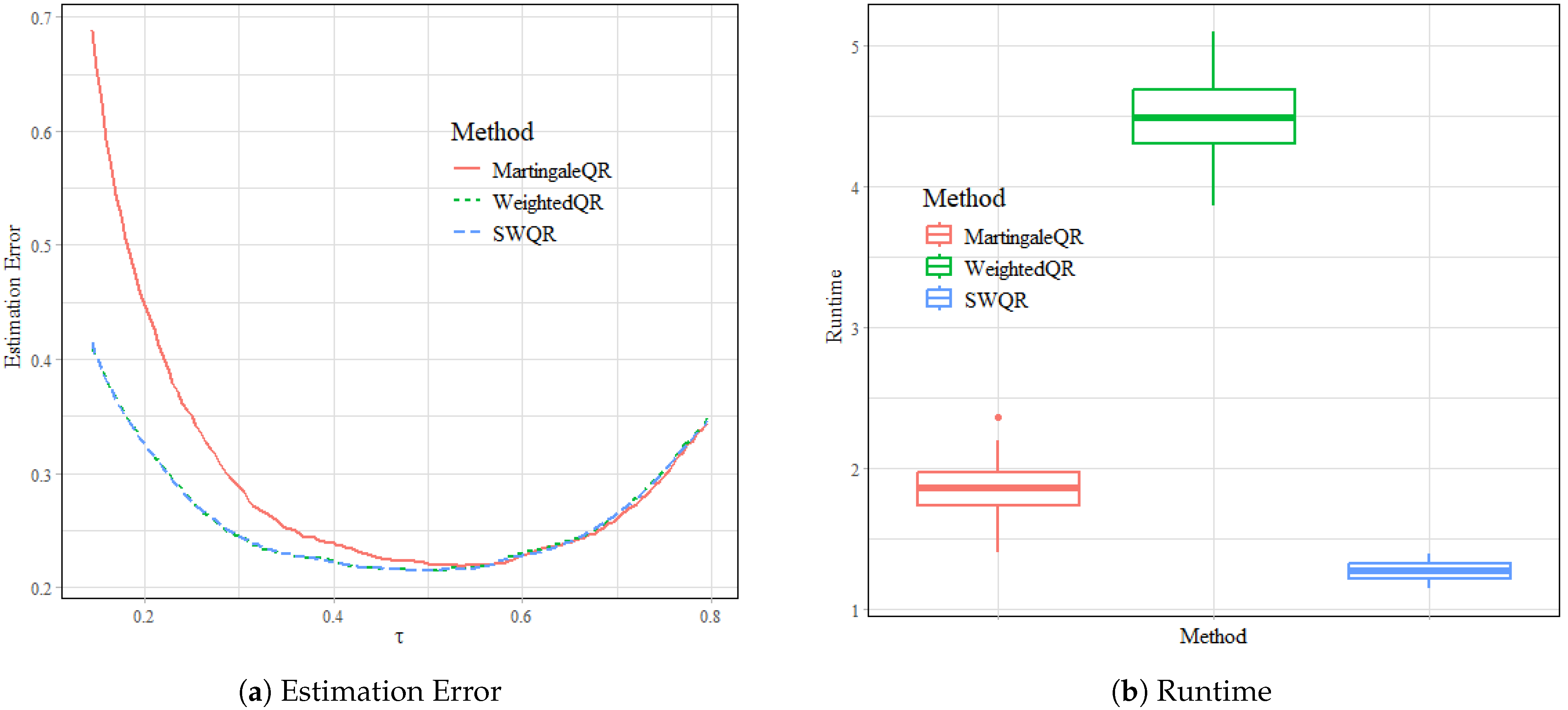
For each quantile level ${\tau }_k$, the estimation is conducted using a quantile grid of ${\left\{{\tau }_k\right\}}_{k=1}^m$ with values ranging from $\{0.05,0.055,0.060,\dots ,0.8\}$. The performance of each method is assessed at every quantile level based on the estimation error, average quantile loss, and runtime.The estimation error is quantified using $\parallel \widehat{\beta }\left({\tau }_k\right)-{\beta }^{*}\left({\tau }_k\right){\parallel }_2$, while the average quantile loss is given by calculating ${\displaystyle \frac{1}{n}}{\sum }_{i=1}^n{\rho }_{{\tau }_k}(y_i-{\widehat{y}}_i)$. We consider three main scenarios (1–3) with different sample sizes and numbers of covariates, each replicated 1000 times. Specifically, we have $n=3000,p=25$ with $p_1=10$ and $p_2=20$, $n=4000,p=35$ with $p_1=14$ and $p_2=28$, and $n=6000,p=50$ with $p_1=20$ and $p_2=40$. In addition to these primary settings, we introduce Scenario 4 specifically designed to evaluate the performance of the proposed method under varying censoring rates. This scenario considers a sample size of $n=4000$ and $p=60$, with $p_1=24$ and $p_2=48$, and examines three censoring levels, 20%, 35%, and 50%. This scenario provides insight into how the degree of censoring impacts estimation accuracy and runtime, further testing the robustness of the proposed method. The acronyms used for the methods are: “SWQR” for our proposed Smoothed Weighted Quantile Regression method, “WeightedQR” for Peng and Huang’s method, and “MartingaleQR” for Portnoy’s method. The results are summarized in the following figures and tables, which show the performance of the three methods.

Figure 1, Figure 2 and Figure 3 provide a comprehensive comparison of estimation error trends and runtimes across the Scenarios 1–3 with varying sample sizes ($n=3000,4000,6000$) and covariate dimensions ($p=25,35,50$). Across all scenarios, SWQR consistently demonstrates competitive performance, achieving estimation errors comparable to or slightly better than WeightedQR and significantly outperforming MartingaleQR, particularly at mid-range quantile levels ($\tau =0.3$ to $\tau =0.6$). The trends indicate that MartingaleQR suffers from higher errors, especially for lower and upper quantile levels, which could be attributed to its less robust handling of censoring effects. These findings confirm that SWQR balances both robustness and accuracy in quantile estimation across all tested conditions. The runtime analysis, as summarized in the corresponding figures, highlights the computational efficiency of SWQR. SWQR consistently requires the least runtime among the three methods, making it the most efficient in scenarios involving larger datasets. WeightedQR, while competitive in terms of estimation error, incurs substantially higher computational costs, particularly as the sample size and covariate dimensionality grow. MartingaleQR exhibits moderate runtimes but suffers from higher estimation errors, making it less suitable for practical applications.

Table 1. Estimation errors and average quantile losses for Scenario 1 with $n=3000$ and $p=25$ at different quantile levels.

$\mathit{\tau }$	Estimation Error			Average Quantile Loss
	MartingaleQR	WeightedQR	SWQR	MartingaleQR	WeightedQR	SWQR
0.2	0.4476	0.3255	0.3257	0.5693	0.5652	0.5658
0.3	0.2882	0.2455	0.2453	0.6494	0.6476	0.6479
0.4	0.2386	0.2230	0.2222	0.6928	0.6919	0.6921
0.5	0.2210	0.2144	0.2151	0.7059	0.7055	0.7056
0.6	0.2287	0.2299	0.2280	0.6907	0.6905	0.6906
0.7	0.2611	0.2656	0.2652	0.6448	0.6447	0.6448

,

Table 2. Estimation errors and average quantile losses for Scenario 2 with $n=4000$ and $p=35$ at different quantile levels.

$\mathit{\tau }$	Estimation Error			Average Quantile Loss
	MartingaleQR	WeightedQR	SWQR	MartingaleQR	WeightedQR	SWQR
0.2	0.4485	0.3442	0.3586	0.5605	0.5565	0.5577
0.3	0.3038	0.2670	0.2733	0.6401	0.6384	0.6389
0.4	0.2494	0.2349	0.2363	0.6838	0.6829	0.6833
0.5	0.2322	0.2237	0.2237	0.6975	0.6970	0.6972
0.6	0.2330	0.2307	0.2309	0.6828	0.6826	0.6826
0.7	0.2646	0.2691	0.2700	0.6379	0.6379	0.6379

and

Table 3. Estimation errors and average quantile losses for Scenario 3 with $n=6000$ and $p=50$ at different quantile levels.

$\mathit{\tau }$	Estimation Error			Average Quantile Loss
	MartingaleQR	WeightedQR	SWQR	MartingaleQR	WeightedQR	SWQR
0.2	0.4563	0.3432	0.3497	0.5542	0.5503	0.5512
0.3	0.3064	0.2650	0.2674	0.6332	0.6316	0.6321
0.4	0.2512	0.2343	0.2369	0.6766	0.6757	0.6762
0.5	0.2317	0.2254	0.2260	0.6906	0.6902	0.6905
0.6	0.2371	0.2378	0.2386	0.6768	0.6766	0.6768
0.7	0.2651	0.2675	0.2674	0.6332	0.6331	0.6333

, featuring estimation errors and average quantile losses, provide insights into the comparative performance of the methods across different scenarios. SWQR achieves average quantile loss values closely aligned with, and often slightly lower than, those of WeightedQR, showcasing its robustness and accuracy in quantile estimation. Notably, in Scenario 3 ($n=6000,p=50$), SWQR maintains its effectiveness despite the increased dataset size, demonstrating scalability and suitability for handling large-scale survival data. MartingaleQR, on the other hand, consistently shows higher average quantile losses and estimation errors. The runtime analysis is summarized in

Table 4. Average runtimes for Scenarios 1–3 with different sample sizes and covariate dimensions.

Average Runtime (in Seconds)	MartingaleQR	WeightedQR	SWQR
$n=3000,p=25$	1.8564	4.4825	1.2736
$n=4000,p=35$	4.2152	10.8706	2.2430
$n=6000,p=50$	11.2568	41.0936	4.4198

. SWQR demonstrates a significant computational advantage over WeightedQR, requiring substantially less time to complete estimation tasks across all scenarios. This is particularly evident in Scenarios 2 and 3, where WeightedQR exhibits a steep increase in runtime as the sample size and covariate dimensionality grow. Although MartingaleQR is computationally efficient, its higher average quantile losses and estimation errors make it less favorable for practical use. The overall balance of accuracy and computational efficiency achieved by SWQR underscores its suitability for large-scale survival analysis, offering a reliable alternative to existing methods when both precision and speed are critical considerations.

In Scenario 4, we evaluated the performance of MartingaleQR, WeightedQR, and SWQR under varying censoring rates (20%, 35%, and 50%, respectively) with $n=4000$ and $p=60$. Figure 4, Figure 5 and Figure 6 depict the estimation errors and runtimes across quantile levels. The results reveal that SWQR consistently outperforms MartingaleQR in terms of estimation error, particularly at lower quantile levels. Compared to WeightedQR, SWQR demonstrates comparable or slightly better estimation performance across all censoring rates, maintaining its robustness even under higher levels of censoring. Furthermore, the increase in censoring rate slightly elevates the estimation error for all methods; however, the relative performance among the methods remains consistent. Regarding runtime, SWQR achieves the lowest computational time across all scenarios, maintaining efficiency regardless of the censoring rate. WeightedQR, in contrast, exhibits significantly higher runtimes, especially under lower censoring rates.

Table 5. Estimation errors and average quantile losses for Scenario 4 with $n=4000$, $p=60$, and 20% censoring at different quantile levels.

$\mathit{\tau }$	Estimation Error			Average Quantile Loss
	MartingaleQR	WeightedQR	SWQR	MartingaleQR	WeightedQR	SWQR
0.2	0.5284	0.4141	0.4098	0.5590	0.5549	0.5550
0.3	0.3643	0.3211	0.3183	0.6399	0.6382	0.6382
0.4	0.2998	0.2806	0.2772	0.6845	0.6836	0.6836
0.5	0.2713	0.2692	0.2672	0.6987	0.6983	0.6983
0.6	0.2829	0.2839	0.2824	0.6847	0.6844	0.6845
0.7	0.3235	0.3294	0.3271	0.6401	0.6400	0.6400

,

Table 6. Estimation errors and average quantile losses for Scenario 4 with $n=4000$, $p=60$, and 35% censoring at different quantile levels.

$\mathit{\tau }$	Estimation Error			Average Quantile Loss
	MartingaleQR	WeightedQR	SWQR	MartingaleQR	WeightedQR	SWQR
0.2	0.5392	0.4231	0.4276	0.5646	0.5606	0.5607
0.3	0.3763	0.3397	0.3394	0.6465	0.6449	0.6449
0.4	0.3147	0.2992	0.2973	0.6917	0.6910	0.6910
0.5	0.2964	0.2937	0.2938	0.7064	0.7060	0.7061
0.6	0.3127	0.3178	0.3169	0.6925	0.6924	0.6924
0.7	0.3736	0.3759	0.3776	0.6481	0.6481	0.6481

,

Table 7. Estimation errors and average quantile losses for Scenario 4 with $n=4000$, $p=60$, and 50% censoring at different quantile levels.

$\mathit{\tau }$	Estimation Error			Average Quantile Loss
	MartingaleQR	WeightedQR	SWQR	MartingaleQR	WeightedQR	SWQR
0.2	0.5593	0.4504	0.4688	0.5652	0.5616	0.5625
0.3	0.4016	0.3688	0.3747	0.6475	0.6462	0.6468
0.4	0.3449	0.3313	0.3359	0.6931	0.6926	0.6929
0.5	0.3285	0.3269	0.3326	0.7081	0.7079	0.7082
0.6	0.3611	0.3614	0.3729	0.6947	0.6948	0.6952
0.7	0.4380	0.4345	0.4538	0.6511	0.6513	0.6517

and

Table 8. Average runtimes for Scenario 4 with $n=4000$ and $p=60$ at different censoring rates.

Average Runtime (in Seconds)	MartingaleQR	WeightedQR	SWQR
20% censoring	11.9355	30.7947	4.2853
35% censoring	9.9623	28.2293	4.5146
50% censoring	7.6677	26.9169	4.8053

provide a detailed numerical comparison, highlighting the estimation errors, average quantile losses, and runtimes for each censoring rate. The average quantile losses for SWQR are closely aligned with those of WeightedQR and remain consistently lower than those of MartingaleQR. This indicates SWQR’s ability to handle data with varying censoring rates effectively. Notably, as the censoring rate increases, the performance gap between WeightedQR and SWQR narrows, with SWQR maintaining its advantage in computational efficiency. In terms of recorded runtime in Table 8, SWQR consistently demonstrates the fastest execution across all censoring levels, highlighting its computational efficiency, while WeightedQR offers competitive accuracy, it suffers from considerably higher computational costs, making it less practical for large-scale applications. MartingaleQR, on the other hand, achieves moderate runtime but struggles with reduced estimation accuracy, particularly under higher censoring rates. This analysis underscores SWQR’s strong balance between speed and accuracy, showcasing its robustness and scalability for datasets with different censoring rates.

In conclusion, the simulation results highlight that the proposed SWQR method consistently surpasses MartingaleQR in estimation accuracy across various quantile levels, particularly as the sample size and number of covariates increase. SWQR balances computational efficiency and estimation accuracy, outperforming WeightedQR, which is limited by its high computational cost in large-scale settings. According to the results, the disparity in runtimes becomes increasingly evident with higher dimensionality, emphasizing SWQR’s capability to deliver reliable performance with minimal computational burden. These results underscore the practicality of SWQR, making it an effective solution for large-scale survival data analysis where both accuracy and resource efficiency are critical considerations.

4.2. Real Data Application

To further evaluate the performance of the proposed smoothed weighted quantile regression method, we applied it to a dataset on primary biliary cirrhosis (PBC), a liver disease dataset extensively used in survival analysis literature [28]. This dataset consists of information on 418 patients, with their survival times either observed or right-censored. The data include clinical measurements such as age, edema status, and biochemical markers (serum bilirubin, albumin, and prothrombin time). Approximately 40% of the patients in the dataset are censored, making it a suitable candidate for testing the robustness and accuracy of censored quantile regression methods. Our aim is to model the relationship between the logarithm of survival time and the selected covariates at different quantile levels. The response variable of interest is the logarithm of survival time, $Y=ln\left(T\right)$, and the covariates include: age of the patient (in years) ($X_1$), edema status ($X_2$), Logarithm of serum bilirubin concentration (mg/dL) ($X_3$), Logarithm of albumin concentration (gm/dL) ($X_4$), Logarithm of prothrombin time (in seconds) ($X_5$). We model the conditional quantile function of the logarithm of survival time at each quantile level $\tau$ as:

$$F_{Y|X}^{-1}\left(\tau \right)={\beta }_0+{\beta }_1{X}_1+{\beta }_2{X}_2+{\beta }_3{X}_3+{\beta }_4{X}_4+{\beta }_5{X}_5,$$

where the regression coefficients ${\beta }_j\left(\tau \right)$ represent the effect of each covariate on the quantile $\tau$ of the survival time distribution. To compare the performance of the SWQR method, we apply MartingleQR and WeightedQR [15,17]. For the SWQR method, a quantile grid ${\left\{{\tau }_k\right\}}_{k=1}^m$ is selected, ranging from 0.05 to 0.80 in increments of 0.05. The estimation of coefficients is performed for each quantile level, and the performance of all three methods was assessed based on the estimated coefficients.

The estimated regression coefficients for each method are computed across the quantile grid, with the results compared in

Table 9. Estimated regression coefficients at different quantile levels.

Estimated Coefficients	MartingleQR	WeightedQR	SWQR
${\widehat{\beta }}_1(\tau =0.2)$	−0.0242	−0.0248	−0.0315
${\widehat{\beta }}_1(\tau =0.3)$	−0.0247	−0.0217	−0.0271
${\widehat{\beta }}_1(\tau =0.4)$	−0.0247	−0.0251	−0.0272
${\widehat{\beta }}_1(\tau =0.5)$	−0.0314	−0.0320	−0.0319
${\widehat{\beta }}_1(\tau =0.6)$	−0.0294	−0.0334	−0.0287
${\widehat{\beta }}_1(\tau =0.7)$	−0.0241	−0.0235	−0.0262
${\widehat{\beta }}_2(\tau =0.2)$	−0.8194	−0.8309	−0.7714
${\widehat{\beta }}_2(\tau =0.3)$	−0.8565	−0.9189	−0.8974
${\widehat{\beta }}_2(\tau =0.4)$	−0.9623	−0.9629	−1.0515
${\widehat{\beta }}_2(\tau =0.5)$	−0.8513	−0.7693	−0.9534
${\widehat{\beta }}_2(\tau =0.6)$	−0.6393	−0.5547	−0.5323
${\widehat{\beta }}_2(\tau =0.7)$	−0.6384	−0.4901	−0.6046
${\widehat{\beta }}_3(\tau =0.2)$	−0.5543	−0.5881	−0.6682
${\widehat{\beta }}_3(\tau =0.3)$	−0.5842	−0.5738	−0.6463
${\widehat{\beta }}_3(\tau =0.4)$	−0.5776	−0.5564	−0.6280
${\widehat{\beta }}_3(\tau =0.5)$	−0.5365	−0.5030	−0.5899
${\widehat{\beta }}_3(\tau =0.6)$	−0.4969	−0.4778	−0.5551
${\widehat{\beta }}_3(\tau =0.7)$	−0.5626	−0.4953	−0.5648
${\widehat{\beta }}_4(\tau =0.2)$	1.7351	1.4623	1.6809
${\widehat{\beta }}_4(\tau =0.3)$	1.7709	1.5881	1.4501
${\widehat{\beta }}_4(\tau =0.4)$	0.9546	0.9600	0.9270
${\widehat{\beta }}_4(\tau =0.5)$	1.2977	1.5140	0.9674
${\widehat{\beta }}_4(\tau =0.6)$	1.3242	1.2769	1.5422
${\widehat{\beta }}_4(\tau =0.7)$	1.3222	1.5836	1.4378
${\widehat{\beta }}_5(\tau =0.2)$	−3.4812	−3.2869	−3.3993
${\widehat{\beta }}_5(\tau =0.3)$	−2.3751	−2.7282	−2.6992
${\widehat{\beta }}_5(\tau =0.4)$	−2.5118	−2.6874	−2.3583
${\widehat{\beta }}_5(\tau =0.5)$	−1.0635	−1.3906	−1.0801
${\widehat{\beta }}_5(\tau =0.6)$	−0.8393	−1.8940	−1.5616
${\widehat{\beta }}_5(\tau =0.7)$	−0.8966	−1.3901	−1.0299

and Figure 7. Each covariate’s impact on survival time was examined, highlighting differences in how the methods handle censored observations. For lower quantiles ($\tau =0.1$ to $\tau =0.3$), the SWQR method closely matches the results from Portnoy [15]’s method in terms of coefficient magnitude and direction, while showing slightly more stability compared to Peng and Huang [17]’s method. For example, the effect of serum bilirubin ($X_3$) on survival time diminishes as we move toward higher quantiles, reflecting how severe cases impact survival time differently across the population. Similarly, the impact of age on survival ($X_1$) shows consistent trends across all methods, with SWQR capturing the effects more consistently across quantiles. At higher quantiles ($\tau =0.6$ and above), the SWQR method continues to provide reliable coefficient estimates, while the performance of Portnoy [15]’s method starts to deteriorate due to challenges with higher censoring. Peng and Huang [17]’s method also encounters computational difficulties, particularly with respect to estimating coefficients for $X_2$ (edema status), as its estimates fluctuate more erratically at these higher quantiles.

In this real-data application, the SWQR method demonstrated its robustness and flexibility in handling censored survival data across a wide range of quantile levels. The method not only provided stable and accurate coefficient estimates, particularly in higher quantiles where censoring becomes more pronounced. The consistent performance of SWQR across different quantile levels, coupled with its computational advantages, makes it a valuable tool for analyzing censored survival data in medical and other applied fields.

5. Discussion and Conclusions

In this study, we introduced smoothed weighted quantile regression, a novel approach designed to address the challenge of right-censored data, commonly encountered in survival analysis. SWQR combines convolution smoothing with quantile regression, offering an efficient solution to the non-differentiability issues inherent in traditional methods, thus enabling gradient-based optimization. By comparing SWQR with two widely used methods, including MartingaleQR and WeightedQR, our findings demonstrate that SWQR is both computationally efficient and robust across various settings.

The results from the simulation study reveal that SWQR generally performs better than MartingaleQR in terms of estimation accuracy, particularly at certain quantile levels and as the sample size and number of covariates increase. Across different quantile levels, SWQR exhibits superior performance, particularly at higher quantiles where the presence of right-censoring can severely degrade the accuracy of other methods. While WeightedQR performs slightly better in terms of accuracy at certain quantiles, it comes at a high computational cost, making it impractical for large-scale data. In contrast, SWQR strikes a balance, maintaining high levels of accuracy while remaining computationally feasible. This balance becomes more evident in large-scale settings, as shown in the simulations with $n=6000$ and $p=50$, where the runtime of WeightedQR increases dramatically, whereas SWQR continues to perform efficiently. These results confirm that SWQR is a scalable and practical method for handling large datasets, making it a valuable tool in applications where computational resources are a constraint. Furthermore, the method’s ability to provide reliable estimates across a broad range of quantile levels is especially advantageous when analyzing the tails of a distribution, where outliers or extreme values may carry significant importance. Additionally, SWQR consistently achieves average quantile losses similar to or slightly lower than those of WeightedQR across different scenarios, highlighting its ability to maintain accuracy while balancing computational costs. This performance is especially notable in Scenario 4, where censoring rates are varied. Under higher censoring rates, SWQR demonstrates robustness and stability in estimation accuracy compared to MartingaleQR, which struggles significantly. WeightedQR maintains high accuracy but with a steep increase in runtime, further emphasizing the advantage of SWQR in practical applications.

The real data application using the PBC dataset provided further validation of SWQR’s practical utility, but its results were relatively consistent with those observed in simulations. While the dataset is of moderate size, SWQR demonstrated stable performance across the quantile spectrum, particularly in cases with heavy censoring. The differences between SWQR, WeightedQR, and MartingaleQR in real data echoed the patterns found in the simulations. SWQR provided more reliable estimates at higher quantiles compared to MartingaleQR, which struggled with heavily censored data. The average quantile loss confirms the utility of SWQR in real-world scenarios, showing its ability to handle heavy censoring without sacrificing estimation quality. The flexibility of SWQR in modeling the distribution of survival times across different quantiles shows its capability for clinical applications where extreme outcomes are crucial, such as identifying high-risk patients. However, since the patterns of covariate effects, such as the diminishing influence of serum bilirubin at higher quantiles, align with known clinical behaviors, the real data application primarily reinforced the findings from the simulations rather than presenting novel insights.

Despite the strengths of SWQR, there remain areas for future research. One notable challenge is the selection of the bandwidth parameter for the smoothing kernel; while the chosen bandwidth performed well in our simulations, more systematic approaches for optimizing this parameter may yield further improvements. Additionally, investigating the performance of SWQR in high-dimensional settings, especially in ultra-high-dimensional scenarios where $p\gg n$, would be a valuable direction for future research to assess its robustness. Furthermore, developing and reporting theoretical results, such as the asymptotic properties of SWQR, could also provide a stronger foundation for its application in survival analysis.

In conclusion, the proposed SWQR method offers a practical and robust approach for quantile regression in the presence of right-censored data. Its ability to balance computational efficiency with high estimation accuracy, even in large-scale settings, makes it a valuable tool in fields such as biomedicine, economics, and beyond. As data complexity continues to grow, the flexibility and scalability of SWQR will be critical for advancing statistical modeling and decision-making in a wide range of applications.