Article

A B-Polynomial Approach to Approximate Solutions of PDEs with Multiple Initial Conditions

by
Muhammad I. Bhatti
1,* and
Md. Habibur Rahman
2
1
Department of Physics and Astronomy, University of Texas Rio Grande Valley, Edinburg, TX 78539, USA
2
Physical Science, West Valley College, Saratoga, CA 95070, USA
*
Author to whom correspondence should be addressed.
Axioms 2024, 13(12), 833; https://doi.org/10.3390/axioms13120833
Submission received: 25 October 2024 / Revised: 22 November 2024 / Accepted: 24 November 2024 / Published: 27 November 2024
(This article belongs to the Special Issue Differential Equations and Related Topics, 2nd Edition)

Abstract

:
In this article, we present a novel B-Polynomial Approach for approximating solutions to partial differential equations (PDEs), addressing the multiple initial conditions. Our method stands out by utilizing two-dimensional Bernstein polynomials (B-polynomials) in conjunction with their operational matrices to effectively manage the complexity associated with PDEs. This approach not only enhances the accuracy of solutions but also provides a structured framework for tackling various boundary conditions. The PDE is transformed into a system of algebraic equations, which are then solved to approximate the PDE solution. The process is divided into two main steps: First, the PDE is integrated to incorporate all initial and boundary conditions. Second, we express the approximate solution using B-polynomials and determine the unknown expansion coefficients via the Galerkin finite element method. The accuracy of the solution is assessed by adjusting the number of B-polynomials used in the expansion. The absolute error is estimated by comparing the exact and semi-numerical solutions. We apply this method to several examples, presenting results in tables and visualizing them with graphs. The approach demonstrates improved accuracy as the number of B-polynomials increases, with CPU time increasing linearly. Additionally, we compare our results with other methods, highlighting that our approach is both simple and effective for solving multidimensional PDEs imposed with multiple initial and boundary conditions.

1. Introduction

We aim to explore and enhance solutions for partial differential equations (PDEs) by addressing their modeling challenges and improving our understanding of complex systems. Our work introduces a novel technique that aims to achieve greater accuracy in solving PDEs and develops efficient numerical methods to tackle the difficulties of finding exact solutions. We seek to provide new insights into modeling dynamic systems, applying our approach to a range of various PDEs, including applications in chaotic systems, financial models, and social issues like poverty. By validating our method through comparisons with exact solutions, we intend to demonstrate its accuracy and reliability, thereby contributing to the advancement of PDE solution techniques and expanding their applications.
Partial differential equations (PDEs) have garnered significant attention due to their versatile applications across various fields such as physics [1], biology [2,3], finance [4], and engineering [5]. This branch of mathematics extends traditional calculus by studying derivatives and integrals of PDEs, which can model complex systems with memory and hereditary properties [6,7]. PDEs are non-local, meaning that the future state of a system depends on both its current and past states. They are particularly useful for modeling dynamic systems, such as falling objects [8,9], disease spread (e.g., COVID-19 and influenza) [10,11], tumor growth [12], and physical systems like the Duffing oscillator [13]. Despite their utility, finding exact solutions to PDEs and related integral equations is challenging, necessitating the development of various numerical methods. Common approaches include the Finite Difference Method (FDM), Finite Element Method (FEM), Finite Volume Method (FVM), and Spectral Methods [14,15]. Additionally, PDEs are applied in fields such as photoelasticity [16], geophysics [17], finance [18], and wind speed data analysis [19], among others [20]. Researchers have also developed numerical techniques like the Method of Lines (MOL), Lattice Boltzmann Method (LBM), Multigrid Method, and Pseudo-Spectral Methods to solve PDEs [21,22,23]. For instance, coupled Burger’s equations [24] deliver more accurate modeling of phenomena such as sedimentation and wave processes [25,26]. The existence and uniqueness of solutions for PDEs are crucial topics, extensively studied through both analytical and numerical methods. Advanced techniques, including sliding mode control (SMC), are employed to handle nonlinear models and ensure stability [27]. PDEs also play a significant role in signal processing [28], statistics [29], and biology [30], with methods like the Monte Carlo Method and Discontinuous Galerkin Method (DGM) developed to address these equations [31]. Spectral methods are powerful tools for finding approximate solutions to PDEs, often utilizing orthogonal polynomials such as Chebyshev polynomials (CPs) [32]. Overall, PDEs have become a vital tool in modern mathematics and computational physics, offering robust methods for modeling and solving complex problems across various disciplines [33].
Chaotic systems, which exhibit complex behavior, have applications in electrical engineering, biology, and physics [20,28,29,34]. PDEs provide new insights into modeling and understanding these chaotic systems. The study of PDEs has been extended to chaotic models in electrical circuits and other dynamic systems [35]. PDEs are also used in biology, physics, chemistry, and engineering [1,36]. The relationship between corruption and poverty has been explored using mathematical models [37,38,39], with PDEs offering new methodologies for understanding and simulating the impact of corruption on poverty [37,39]. Nonlinear science, which studies phenomena unique to nonlinear systems, includes research on solutions, bifurcation behavior, and chaotic periodic behavior of nonlinear PDEs [40]. The Gerdjikov–Ivanov equation, for example, is studied for its applications in optics, water waves, and quantum field theory [41,42,43]. Integrating PDEs with chaos theory has expanded the scope of mathematical modeling, providing deeper insight into complex and dynamic systems [40,41,44]. This integration has significant implications for both theoretical research and practical applications in science and engineering [44].
This paper presents an approach to solving PDEs and applies this method to five different examples of PDEs. In a previous study [45,46,47], we explored various approaches to solving both linear and nonlinear partial and fractional differential equations. Building on that foundation, we now use our innovative technique to tackle these PDEs. Each example has an exact solution, and we will compare our estimated solutions with these exact ones. For each example, we present tables and graphs to illustrate the comparison between estimated and exact solutions, demonstrating the accuracy of our approach to solving PDEs.

2. Methodology

The proposed approach unfolds in two main steps:
  • Integration and Condition Incorporation: The first step involves systematically integrating the linear PDE while accommodating all specified initial and boundary conditions. This integration is crucial as it reformulates the problem, allowing the conditions to be incorporated into the structure of the equation, thus ensuring that the solutions adhere to these constraints.
  • Approximation via B-Polynomials: The second step entails expressing the approximate solution using B-polynomials. B-polynomials are particularly advantageous due to their properties of preservation under linear transformations and their ability to provide good approximations for smooth functions. We formulate the approximate solution as a linear combination of B-polynomials, where the unknown coefficients are then determined using the Galerkin finite element method (FEM). This method involves projecting the PDE onto a finite-dimensional space spanned by the B-polynomials, leading to a system of algebraic equations that can be solved efficiently using modern computers. The Bernstein basis polynomials of degree n are defined as follows [46]:
    B i , n = n i x i R x n i R n ,               0 i n
    where n i denotes the binomial coefficient:
    n i = n ! i ! n i !
Here, n ! represents the factorial n, and i ! denotes the factorial of i , for values of i ranging from 0 to n . The parameter R indicates the upper limit of the interval 0 , R , within which the polynomials are defined, thereby forming a complete basis set. For any degree n, there are n + 1 Bernstein polynomials. For simplicity, we define B i , n x = 0 when i < 0 or i > n . A straightforward coding in Mathematica or Maple can be used to generate all non-zero Bernstein polynomials of any degree n that are supported within this interval. The approximate solution to the partial differential equation can be expressed as a linear combination of Bernstein polynomials.
y   x ,   t = i , j n , m C i j   B i x   B j t .
3.
We consider the following equation as a typical partial differential equation [48].
U t + 1 2 U x = 0 .
The above equation is subject to an initial condition,   U x , 0 , to ensure a unique solution. As the first step, we integrate both sides of Equation (2) with respect to the variable t . This integration accounts for both terms and incorporates the given initial condition.
0 t U t d t + 1 2   0 t U x   d t = 0 U x , t U x , 0 + 1 2   0 t U x   d t = 0 U x , t + 1 2   0 t U x   d t = U x , 0
By substituting Equation (1) into Equation (3), we derive the operational matrix equation M   C = W . This equation is solved numerically to find the unknown coefficients C, which are then substituted back into Equation (1) to obtain the final numerical solution.

3. Application

We shall apply our approach to approximate solutions of various PDEs considered below. The results of these examples are presented in tables and graphs to illustrate accuracy. All calculations and graphs are carried out with Mathematica 14.1 [49]. An approximate solution and error analysis are provided for each example considered.
Example 1. 
Let us analyze the following partial differential equation:
y t + 1 2 y x = 0 .
This is specified with an initial condition  y x , 0 = x 3  to obtain a unique solution. The exact solution of Equation (4) is given by    y e x a c t x ,   t = ( x t 2 ) 3 . As a first step, we integrate both sides of Equation (4). The integration of both terms with respect to the variable  t  is provided, along with incorporating one initial condition:
y   x , t + 1 2   0 t y x   d t = x 3 .
By substituting Equation (1) into Equation (5), we obtain the following:
C i j   B i x   B j t + 1 2   0 t C i j   B i x B i t   d t = x 3 .
By taking the scalar product with B-polys   B k x   B l t and integrating on both sides, we obtain the following:
C i j   B i x B k x B j t B l t + 1 2   B i x B k x B j ¯ t B l t                                                                                                 = x 3     B k x     B l t   .
where the matrices are defined below:
M = M x   M t + 1 2   N x   N t M x = B i x B k x M t = B i t B l t N x = B i x B k x N t = B j ¯ t B l x B ¯ t = 0 t B j t d t     W = x 3     B k x     B l t   .
Eventually, the equation  M   C = W  is solved numerically for unknown coefficients C, which are inserted in Equation (1) to determine the solution. The final numerical solution of Equation (4) is provided:
y x ,   t = C i j   B i x   B j t = 1.0 x 3 ± 1.5 x 2 t 0.125   t 3 + 0.75 x t 2 .
This solution precisely matches the exact solution, illustrating the effectiveness of the current approach. For this example, we also present the tables related to this solution and a graph to compare with the exact solution of the example.
In Table 1 and Table 2, the approximate solution calculated using our proposed method for various values of x and at fixed values of t = 1 and t = 0.5 closely align with the exact solution. This strong correspondence demonstrates the accuracy of our technique and its ability to deliver precise results. The consistent agreement between the approximate and exact values under different conditions further highlights the effectiveness of our method in yielding reliable outcomes.
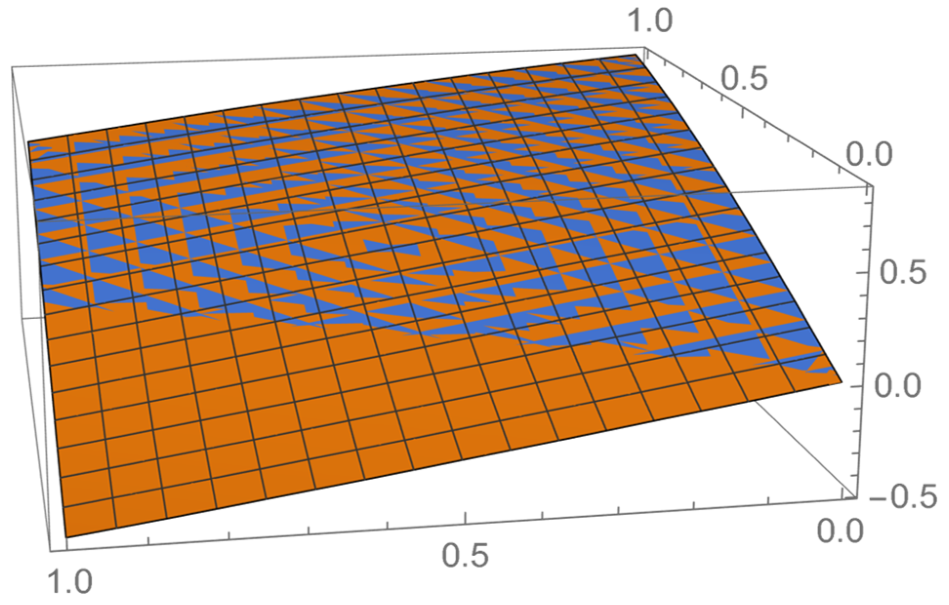
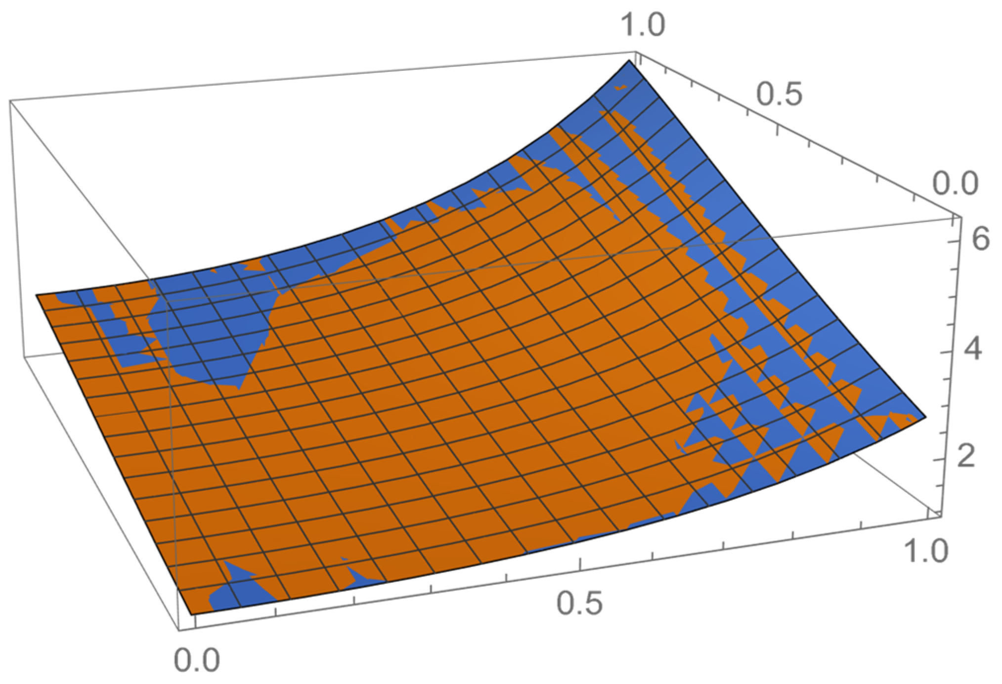
The approximate 3D solution, U(x), and the exact solution are depicted in Figure 1. This visual representation highlights the significant overlap between the two solutions, which is an indication that the solution is accurate.
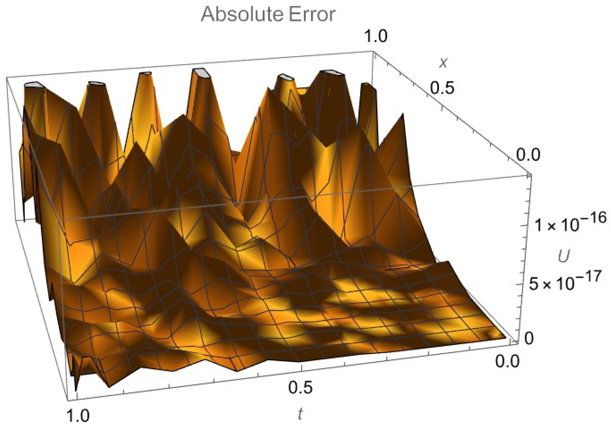
In Figure 1 and Figure 2, the graph produced by our approximate approach closely aligns with the exact solution for various values of x and t , with both graphs nearly overlapping. The error margin, approximately 10−17, underscores the high accuracy of our method. This exceptionally small error margin highlights the precision of our technique, demonstrating its ability to deliver remarkably accurate and reliable results.
Example 2. 
Let us investigate the solution of another partial differential equation in the interval [0, 1]:
2 y t + y x = 0 ,
This is subjected to an initial condition,  y x , 0 = sin x . The exact solution of Equation (8) is given by  y e x a c t x ,   t = sin x t 2 . Let us integrate the equation on both sides with respect to variable t   as given below:
2   y   x , t 2   y   x , 0 +   0 t y x   d t = 0 .
This equation can be further simplified after applying the initial condition:
2 y   x , t + 0 t y x   d t = 2 sin x .
We approximate the solution of this equation using the B-polys in two variables  ( x ,   t )  as we did in Example 1,  y   x ,   t = i , j n , m C i j   B i x   B j t . By substituting this approximate solution into Equation (12), we may obtain the following:
2 C i j   B i x   B j t +   0 t C i j   B i x B i t   d t = 2 sin x .
By taking the scalar product with B-polys   B k x   B l t  and integrating on both sides, we obtain the following:
C i j   2 B i x B k x   B j t B l t +   B i x B k x   B j ¯ t B l t = 2 sin x   B k x     B l t   .
where matrices are defined as follows:
M = M x   M t + N x   N t M x = B i x B k x M t = B i t B l t N x = B i x B k x N t = B j ¯ t B l x B ¯ t = 0 t B j t d t W = 2 sin x     B k x     B l t   .
Eventually, Equation (14),  M   C = W , is solved numerically for unknown coefficients C, which are inserted back in Equation (1) to determine the numerical solution. The final numerical solution of Equation (10) is provided:
y a p p r o x x ,   t = 0.999999 x 0.16667 x 3 + 5 × 10 5 x 4 + 0.00832 x 5 + 2.2 × 10 5 x 6 2.2 × 10 4 x 7 + 1.2 × 10 5 x 8 + t ( 0.499999 + 0.2500 x 2 9 × 10 6 x 3 0.020801 x 4 6.5 × 10 5 x 5 + 7.70 × 10 4 x 6 4.7 × 10 5 x 7 ) + t 3 ( 0.020833 2.2949 × 10 6 x 0.0104 x 2 5.4502 × 10 5 x 3 + 9.6293 × 10 4 x 4 8.2688 × 10 5 x 5 ) + t 5 2.600121 × 10 4 4.0877 × 10 6 x + 1.4444 × 10 4 x 2 2.067191 × 10 5 x 3 + 1.7195 × 10 6 + t 6 2.4073 × 10 5 x + 5.167977 × 10 6 x 2 + t 4 ( 0.0026 x + 2.0438 × 10 5 x 2 4.8146 × 10 4 x 3 + 5.1680 × 10 5 x 4 ) + t 2 ( 0.1250 x + 0.020801 x 3 + 8.1753 × 10 5 x 4 0.001156 x 5 + 8.2688 × 10 5 x 6 )
The solution of Example 2 is compared with the exact solution, illustrating the effectiveness of the current approach. We also present the tables related to this solution and a graph to compare with the exact solution of the example.
In Table 3 and Table 4, for a range of x values and fixed t values of 1   and 0.5 , the approximate results produced by our proposed method closely correspond to the exact solutions. This close alignment demonstrates the precision of our technique, confirming that it delivers highly accurate results. The consistency between the approximate and exact values across different conditions highlights the reliability and effectiveness of our approach in generating precise outcomes. A similar type of observation is made in the simulations of the graphs presented in Figure 3 and Figure 4.
In Figure 3 and Figure 4, for various values of x and t , the graph produced by our approximate method shows both graphs almost completely overlapping the solutions. The error margin is approximately 10 6 , which affirms that our technique achieves accuracy as we increase the number of B-polys in the expansion Equation (1). This small error margin highlights the precision of our method, demonstrating its effectiveness in providing highly accurate results even in complex scenarios.
Example 3. 
Let us consider a partial differential equation subjected to two initial conditions:
2 y t 2 2 y x 2 = 0 ,
The initial conditions are  y x , 0 = x 2  and  y x , 0 t = 4   x 3 . The exact solution to Equation (17) is given by  y e x a c t x ,   t = x 2 + t 2 + 4 x 2 t + 4 x   t 3 . Let us integrate Equation (17) twice with respect to   t  on both sides. By implementing both initial conditions, we obtain the following:
y   x , t   0 t 0 t 2 y x 2 d t d t = x 2 4 x 3 t .
We approximate the solution of this equation using the B-polys in two variables  ( x ,   t )  as we did in Example 1,  y   x ,   t = i , j n , m C i j   B i x   B j t . By substituting this approximate solution into Equation (18), we may obtain the following
C i j   B i x   B j t C i j     0 t 0 t B i x B j t d t d t = x 2 4 x 3 t .
By taking the scalar product with B-polys   B k x   B l t  and integrating on both sides, we obtain the following
C i j   B i x B k x B j t B l t   B i x B k x   B j ¯ ¯ t B l t = x 2 4 x 3 t     B k x     B l t .
where matrices are defined as follows:
M = [ M x   M t   N x   N t ]   M x = B i x B k x M t = B i t B l t N x = B i x B k x N t =   B j ¯ ¯ t B l t B ¯ ¯ t = 0 t d t   0 t B j t t d t W = x 2 4 x 3 t     B k x     B l t   .
Eventually, Equation (20),  M   C = W , is solved numerically for unknown coefficients C, which are inserted back in Equation (1) to determine the numerical solution. The final numerical solution of Equation (17) is provided:
y a p p r o x x ,   t = 1.0 x 2 + 4.0 x 3 t + t 2 + 4.0 x t 3 .
The solution of Example 3 is compared with the exact solution, illustrating the effectiveness of the current approach. We also present Table 5 and Table 6 related to this solution and graphs to compare with the exact solution of this example.
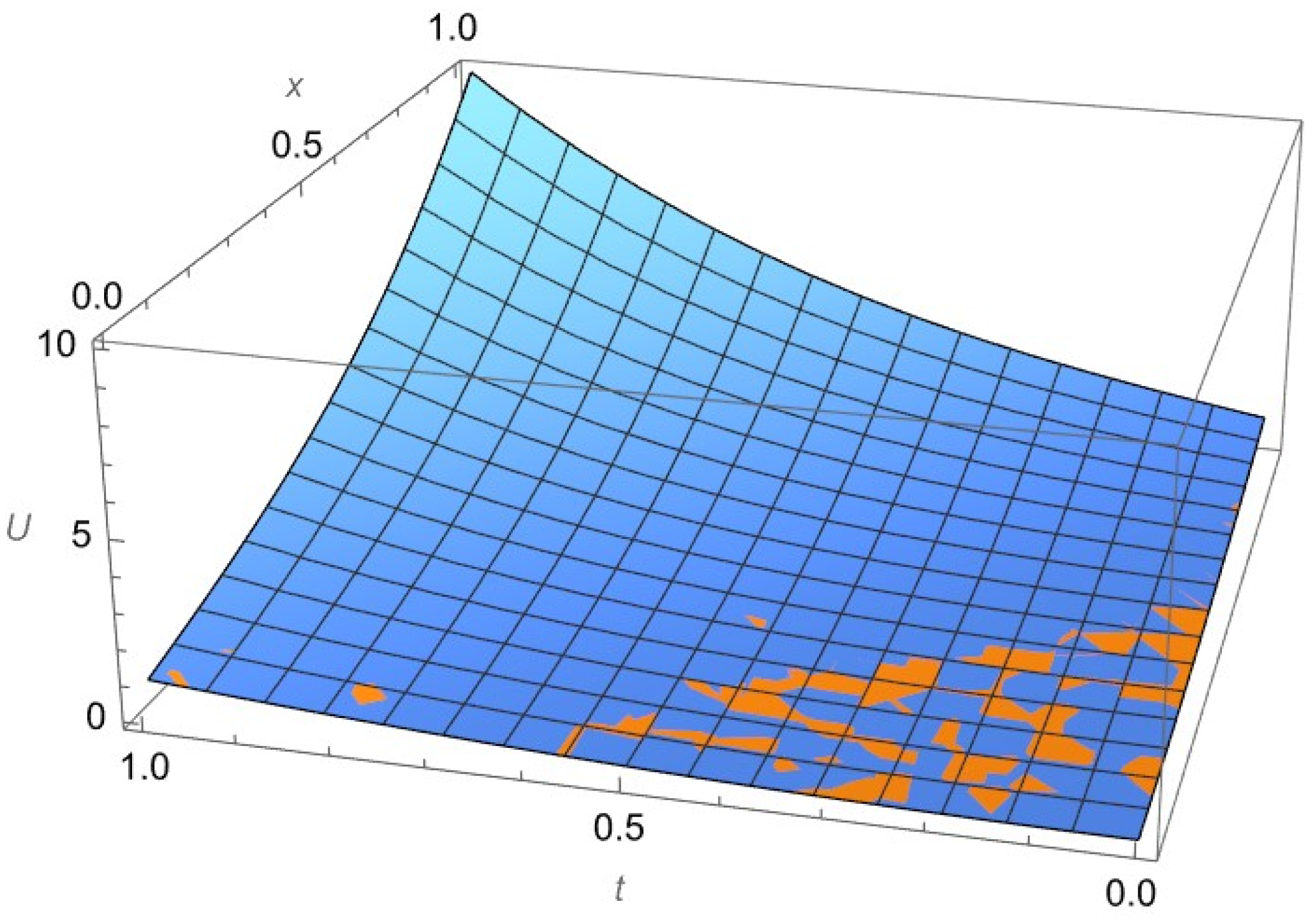
In Table 5 and Table 6, for a range of x values and fixed t values of 1 and 0.5 , the approximate results produced by our proposed method closely correspond to the exact solutions. This close alignment demonstrates the precision of our technique, confirming that it delivers highly accurate results. The consistency between the approximate and exact values across different conditions highlights the reliability and effectiveness of our approach in generating precise outcomes. A similar type of observation is made in the simulations of the presented graphs in Figure 5 and Figure 6.
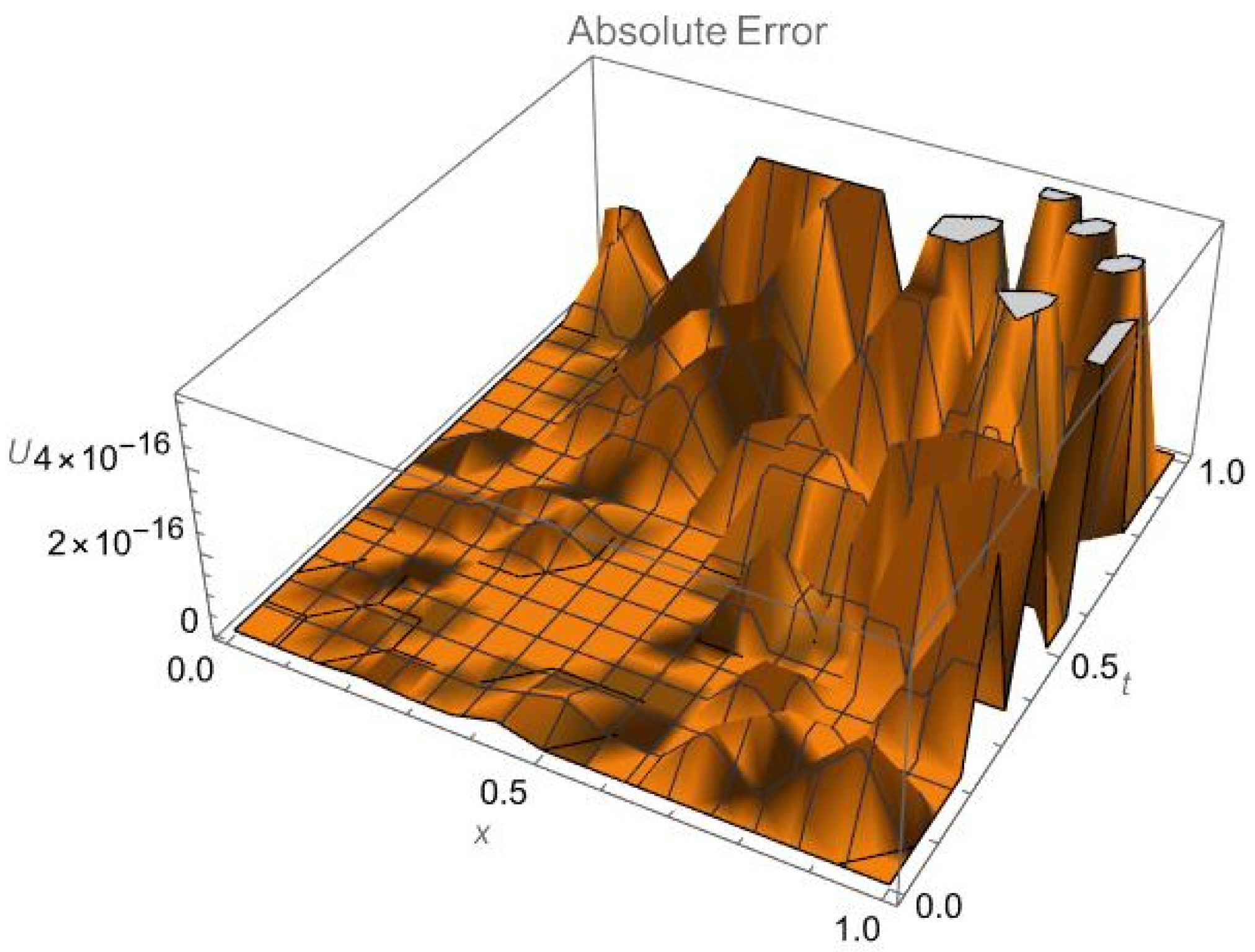
In Figure 5 and Figure 6, for various values of x and t , the graph produced by our approximate method shows both graphs almost completely overlapping the solutions. The error margin is approximately 10 16 , which affirms that our technique achieves accuracy as we increase the number of B-polys in the expansion Equation (1). This small error margin highlights the precision of our method, demonstrating its effectiveness in providing highly accurate results, even in complex scenarios.
Example 4. 
Consider a partial differential equation subjected to two initial conditions:
2 y x 2 + 2 x   y x 6 + 4 x 2 cos t y d y d t = 0 ,
The initial conditions are  y 0 , t = e sin t  and  y 0 , t t = 0 . The exact solution of Equation (23) is known,  y e x a c t x ,   t = e x 2 + sin t . To implement these two initial conditions, we shall integrate Equation (23) twice with respect to variable  x  on both sides to obtain the following:
x   y x , t 0 x d x 0 x 6   x + 4   x 3 x cos t y x , t d x 0 x d x 0 x y t d x = x   e sin t .
We approximate the solution of Equation (21) using the 2D B-polys in two variables  ( x ,   t )  by substituting Equation (1) into Equation (24); we obtain the following:
C i j   x   B i x B k x B j t B l t B ~ i x B k x B j t B l t B i ¯ x B k x B ˙ j t B l t = x   e sin t   B k x     B l t .
Let us consider the following:
M = [ M x   M t N x   M t M x   N t ] M x = x   B i x B k x M t = B i t B l t N x = B ¯ i x B k x N t = B ˙ j t B l x B ¯ x = 0 x d x 0 x x   B i x d x     B ~ x = 0 x d x 0 x 6   x + 4   x 3 x cos t B i x d x     W = x   e sin t   B k x     B l t   .
Equation (23),  M   C = W , is solved numerically for unknown coefficients C, which are inserted back in Equation (1) to determine the numerical solution. The final numerical solution of Equation (23) is provided:
y a p p x ,   t = 1   1.5337 × 10 5 x + 1.0003 x 2 0.0038166 x 3 + 0.523579 x 4 0.089481 x 5 + 0.383877 x 6 0.340612 x 7 + 0.378973 x 8 0.195371 x 9 + 0.060799 x 10 + t 7 ( 1.9903 × 10 3 + 1.4262 × 10 2 x 0.2476 x 2 + 1.4980 x 3 7.159592 x 4 + 24.3382 x 5 51.5538 x 6 + 66.4255 x 7 50.8696 x 8 + 21.3534 x 9 3.7930 x 10 ) + t 5 ( 6.8923 × 10 2 + 9.2563 × 10 3 x 0.2322 x 2 + 0.9766 x 3 4.0170 x 4 + 11.4046 x 5 21.6208 x 6 + 26.2868 x 7 19.7453 x 8 + 8.3355 x 9 1.5141 x 10 ) + t 9 ( 4.7210 × 10 3 + 1.8164 × 10 3 x 3.5166 × 10 2 x 2 + 0.1982 x 3 1.0419 x 4 + 3.6543 x 5 7.7393 x 6 + 9.8216 x 7 7.3552 x 8 + 3.0070 x 9 0.51917 x 10 ) + t 3 ( 9.1306 × 10 5 + 8.3258 × 10 4 x 1.6402 × 10 2 x 2 + 1.2477 × 10 1 x 3 5.3865 × 10 1 x 4 + 1.4841 x 5 2.6714 x 6 + 3.1080 x 7 2.2458 x 8 + 9.1521 × 10 1 x 9 1.6065 × 10 1 x 10 ) + t ( 9.999999 × 10 1   1.067340 × 10 5 x + 1.000237 x 2 2.907322 × 10 3 x 3 + 5.197151 × 10 1 x 4 7.781846 × 10 2 x 5 + 3.595589 × 10 1 x 6 3.0859569 × 10 1 x 7 + 3.540284 × 10 1 x 8 1.848975 × 10 1 x 9 + 5.897159 × 10 2 x 10 ) + t 2 ( 5.0001 × 10 1 8.2944 × 10 5 x + 5.0223 × 10 1 x 2 2.063 × 10 2 x 3 + 3.511569 × 10 1 x 4 3.1266 × 10 1 x 5 + 7.0819 × 10 1 x 6 7.9842 × 10 1 x 7 + 6.5310 × 10 1 x 8 2.8693 × 10 1 x 9 + 6.3182 × 10 2 x 10 ) + t 4 ( 1.2442 × 10 1 3.698945 × 10 3 x 5.8433 × 10 2 x 2 4.328532 × 10 1 x 3 + 1.676118 x 4 4.609897 x 5 + 8.060321 x 6 9.265422 x 7 + 6.684240 x 8 2.757139 x 9 + 4.922808 × 10 1 x 10 ) + t 8 ( 1.444032 × 10 2   7.819558 × 10 3 x + 1.486302 × 10 1 x 2 8.394227 × 10 1 x 3 + 4.258852 x 4 14.853298 x 5 + 31.6631537 x 6 40.635425 x 7 + 30.836015 x 8 12.787505 x 9 + 2.240430 x 10 ) + t 6 ( 1.496595 × 10 3   1.457529 × 10 2 x + 2.589747 × 10 1 x 2 1.506723 x 3 + 6.642227 x 4 21.145270 x 5 + 43.300027 x 6 55.082780 x 7 + 42.188095 x 8 17.852263 x 9 + 3.212182 x 10 ) .
The solution of Example 4 is compared with the exact solution, illustrating the effectiveness of the current approach. We also present Table 7 and Table 8 related to this solution and the graphs to compare with the exact solution of Example 4.
In both Table 7 and Table 8, we observe that for a range of x values and fixed values of t at 0.5 and 1.0 , the approximate results obtained using our proposed method are in close agreement with the exact solution. This close correspondence between the calculated values and the exact results illustrates the precision and reliability of our approach. The method’s effectiveness in consistently yielding such accurate results across different parameters further emphasizes its robustness and potential for solving similar problems. Overall, the data confirms that the proposed technique delivers results with a high degree of accuracy.
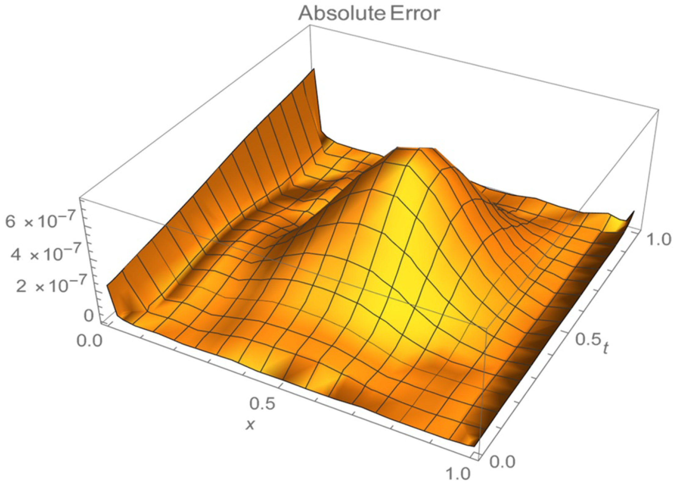
In Figure 7 and Figure 8, the graphs generated by our approach show a remarkable alignment with the exact solution across different values of x and t. The close overlap between the two graphs indicates that our method produces results almost indistinguishable from the exact ones. The error margin is very small, on the order of 10 7 , which underscores the precision of our approach only using 10 B-polys. Such a minimal error range demonstrates the technique’s capability to generate highly accurate outcomes, making it a reliable tool for solving complex problems where precision is critical. This level of accuracy further validates the robustness and effectiveness of the method.
Example 5. 
Finally, let us consider a partial differential equation subjected to two initial conditions:
2 y x 2 + 2 x   y x 5 + 4 x 2 y 2 y t 2 = 0 ,
where the initial conditions are  y ( 0 , t ) = e t  and  y ( 0 , t ) t = 0 . The exact solution of Equation (27) is well known,  y e x a c t x ,   t = e x 2 t . Furthermore, in order to implement two initial conditions, we need to integrate Equation (27) twice with respect to variable x on both sides to obtain the following:
x   y   x , t 0 x d x   0 x 5   x + 4   x 3 y x , t d x 0 x d x   0 x x   2 y t 2   d x = x   e t .
We approximate the solution of Equation (27) using the 2D B-polys in two variables  ( x ,   t )  and by substitute Equation (1) into Equation (28), we obtain the following:
C i j   [ x   B i x B k x B j t B l t B ~ i x B k x B j t B l t   B i ¯ x B k x B ¨ j t B l t ] = x   e t   B k x     B l t   .
where
M = [ M x   M t N x   M t N N x   N t ] M x = x   B i x B k x M t = B i t B l t N x = B ¯ i ( x ) B k x N N x = B ~ i ( x ) B k x N t = B ¨ j ( t ) B l x B ¯ x = 0 x d x 0 x x   B i x d x     B ~ x = 0 x d x 0 x ( 5   x + 4   x 3 )   B i x d x     W = x   e t   B k x     B l t   .
Equation (29),  M   C = W , is solved numerically for unknown coefficients C, which are inserted in Equation (1) to determine the numerical solution. The final numerical solution of Equation (27) is provided:
y e s t i m a t e x ,   t = 1   1.5307 × 10 5 x + 1.0003 x 2 3.8115 × 10 3 x 3 + 5.2355 × 10 1 x 4 8.9367 × 10 2 x 5 + 3.8362 × 10 1 x 6 3.4027 × 10 1 x 7 + 3.7871 × 10 1 x 8 1.9526 × 10 1 x 9 + 6.0779 × 10 2 x 10 + t 6 ( 1.3827 × 10 3 + 2.5764 × 10 3 x + 2.7753 × 10 2 x 2 2.6650 × 10 1 x 3 + 8.6113 × 10 1 x 4 6.1690 × 10 1 x 5 2.7592 x 6 + 7.6330 x 7 8.3219 x 8 + 4.3349 x 9 0.8925 x 10 ) + t 8 ( 1.4911 × 10 5   + 8.2808 × 10 4 x + 1.1583 × 10 2 x 2 1.3686 × 10 1 x 3 + 4.4215 × 10 1 x 4 2.4383 × 10 1 x 5 1.6538 x 6 + 4.3088 x 7 4.6792 x 8 + 2.4717 x 9 0.5212 x 10 ) + t 4 ( 4.1656 × 10 2   + 7.5081 × 10 4 x + 5.1498 × 10 2 x 2 7.3228 × 10 2 x 3 + 2.5474 × 10 1 x 4 3.2729 × 10 1 x 5 8.3619 × 10 2 x 6 + 9.0175 × 10 1 x 7 1.1633 x 8 + 6.4634 × 10 1 x 9 1.3615 × 10 1 x 10 ) + t ( 1 + 1.5482 × 10 5 x 1.0003 x 2 + 3.7612 × 10 3 x 3 5.2330 × 10 1 x 4 + 8.8756 × 10 2 x 5 3.8267 × 10 1 x 6 + 3.3929 × 10 1 x 7 3.7801 × 10 1 x 8 + 1.9496 × 10 1 x 9 6.0721 × 10 2 x 10 ) + t 3 ( 1.6666 × 10 1 1.6549 × 10 4 x 1.6882 × 10 1 x 2 + 1.4763 × 10 2 x 3 1.3818 × 10 1 x 4 + 1.3484 × 10 1 x 5 2.2391 × 10 1 x 6 + 1.5206 × 10 1 x 7 5.5219 × 10 2 x 8 3.6389 × 10 3 x 9 + 2.0082 × 10 3 x 10 ) + t 2 ( 4.999996 × 10 1   + 6.7792 × 10 6 x + 5.0022 × 10 1 x 2 1.8090 × 10 3 x 3 + 2.6235 × 10 1 x 4 5.5427 × 10 2 x 5 + 2.2719 × 10 1 x 6 2.2255 × 10 1 x 7 + 2.2886 × 10 1 x 8 1.1202 × 10 1 x 9 + 3.2267 × 10 2 x 10 ) + t 9 ( 1.1383 × 10 6 1.2495 × 10 4 x 2.7674 × 10 3 x 2 + 3.1234 × 10 2 x 3 9.5808 × 10 2 x 4 + 3.6723 × 10 2 x 5 + 4.0160 × 10 1 x 6 9.9298 × 10 1 x 7 + 1.0657 x 8 5.6300 × 10 1 x 9 + 1.1942 × 10 1 x 10 ) + t 5 ( 8.3233 × 10 3 1.8273 × 10 3 x 2.9144 × 10 2 x 2 + 1.7729 × 10 1 x 3 5.5883 × 10 1 x 4 + 4.9753 × 10 1 x 5 + 1.3306 x 6 4.0847 x 7 + 4.5375 x 8 2.3662 x 9 + 4.8359 × 10 1 x 10 ) + t 7 ( 1.8928 × 10 1 2.0502 × 10 3 x 2.2313 × 10 2 x 2 + 2.5376 × 10 1 x 3 8.3520 × 10 1 x 4 + 5.4209 × 10 1 x 5 + 2.9014 x 6 7.8195 x 7 + 8.5263 x 8 4.4796 x 9 + 9.3494 × 10 1 x 10 ) .
In both Table 9 and Table 10, for a range of x values and fixed t   values of 0.5 and 1.0 , the approximate values derived from our proposed method show a strong correspondence with the exact solutions. The overlap between the calculated and exact values highlights the precision of our approach. This consistency across different parameters reinforces the reliability of the technique, demonstrating its ability to maintain accuracy even when applied to varying conditions. The close alignment of results serves as clear evidence that our method is not only effective but also highly accurate, making it a valuable tool for solving complex problems with confidence.
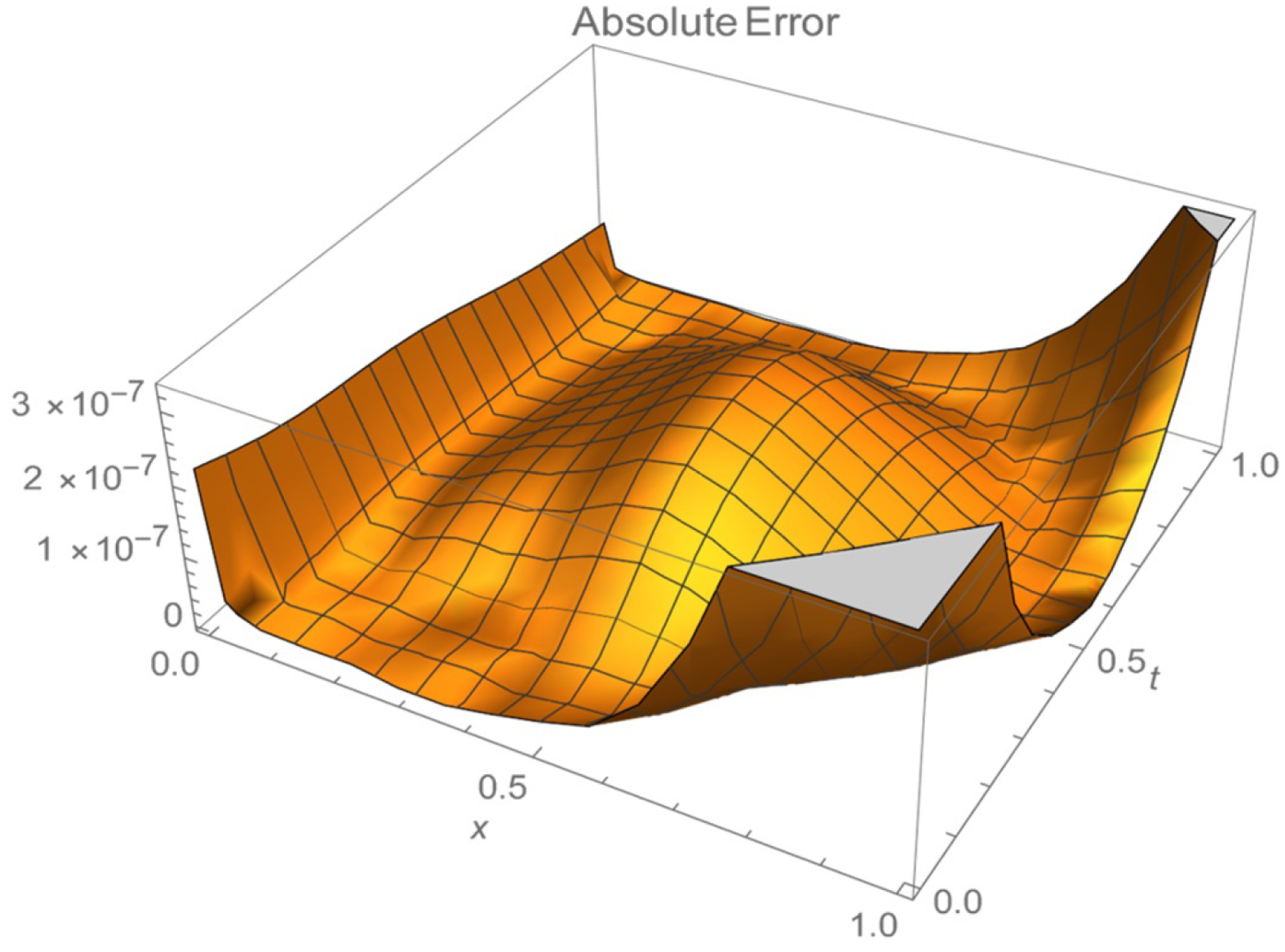
In Figure 9 and Figure 10, across different values of x and t , the graphs produced by our approximate approach closely match the exact solutions, with both graphs nearly overlapping. This close alignment highlights the effectiveness of our method in achieving highly accurate results. The error margin, which is on the order of 10 7 , underscores the exceptional accuracy of our technique. Such a minimal error range reflects the robustness of our approach, demonstrating that it consistently delivers highly accurate outcomes even in complex scenarios. This high degree of precision confirms the reliability and effectiveness of our method for detailed and exact problem-solving.

4. Results

The implementation of this method yielded several promising results: We found that the B-polynomial-based approach provided highly accurate approximations of solutions across a wide range of linear PDEs with diverse initial and boundary conditions. Comparative studies against existing numerical methods indicated superior accuracy and convergence rates. The technique demonstrated robust performance in handling complex problems, including cases with non-homogeneous boundary conditions and varying coefficients. This flexibility underscores the versatility of B-polynomials in approximating solutions under various scenarios. The operational matrices associated with B-polynomials facilitated the transformation of the PDE into algebraic equations quickly and efficiently. As a result, our approach significantly reduced the computational burden typically associated with conventional finite element methods, allowing for faster simulations without sacrificing accuracy.

5. Implications

The implications of our findings are substantial. By successfully incorporating multiple initial and boundary conditions, our technique expands the toolkit available for researchers and practitioners working with linear PDEs. The advantages of using B-polynomials may lead to novel applications in fields such as fluid dynamics, heat transfer, and financial mathematics, where accurate solutions to PDEs are paramount.
Additionally, the integration of the Galerkin method with B-polynomials opens avenues for future exploration and customization of the approach to nonlinear PDEs and higher-dimensional problems. This adaptability positions our methodology as a valuable contribution to the broader field of computational mathematics.

6. Conclusions

In conclusion, this paper presents a comprehensive and effective computational technique for approximating solutions to linear PDEs using two-dimensional Bernstein polynomials. Our method not only addresses the complexities associated with multiple initial and boundary conditions but also enhances both accuracy and computational efficiency. The results verify the effectiveness of our approach, setting the stage for future advancements in solving a broader class of partial differential equations.
The technique exhibits improved accuracy with an increasing number of B-polynomials, with CPU time increasing linearly, highlighting its computational efficiency. The accuracy is validated by comparing approximate solutions with exact ones, demonstrating a close match across various conditions. Tables and graphs in the paper show that the approximate values align closely with the exact solutions, with an error margin on the order of 10−17, indicating exceptional precision. Furthermore, the method’s performance is compared with other approaches, revealing it to be more straightforward and more effective for solving multidimensional PDEs with multiple initial and boundary conditions. Overall, the results underscore the method’s robustness, accuracy, and potential as a powerful tool for addressing complex PDE problems in a range of applications.

Author Contributions

Conceptualization, M.I.B.; software, M.I.B.; methodology, M.I.B.; formal analysis, M.I.B. and M.H.R.; validation, M.I.B. and M.H.R.; data curation, M.I.B. and M.H.R.; resources, M.I.B.; project administration, M.I.B.; investigation, M.I.B. and M.H.R.; supervision, M.I.B.; writing—original draft preparation, M.I.B. and M.H.R.; writing—review and editing, M.I.B. and M.H.R. All authors have read and agreed to the published version of the manuscript.

Funding

There was no external support for this study.

Data Availability Statement

The information supporting the conclusions of this investigation is accessible in the publication.

Acknowledgments

The departmental computing resources used to calculate the findings of this study are gratefully acknowledged.

Conflicts of Interest

The authors declare that they have no known competing financial interests or personal relationships that could have appeared to influence the work reported in this paper.

References

  1. Sommerfeld, A. Partial Differential Equations in Physics. 1949. Available online: https://books.google.com/books?hl=en&lr=&id=PFsDVARE4C0C&oi=fnd&pg=PP1&dq=partial+differential+equations+in+physics&ots=I7LpXtnCrq&sig=t5Sq4nDcIZxgIc5ojuelGWpz45k (accessed on 7 September 2024).
  2. MSimpson, J.; McCue, S.W. Fisher-KPP-type models of biological invasion: Open source computational tools, key concepts and analysis. arXiv 2014, arXiv:2403.01667. [Google Scholar]
  3. Li, W.; Carvalho, R. Automating the Discovery of Partial Differential Equations in Dynamical Systems. arXiv 2024, arXiv:2404.16444v1. [Google Scholar] [CrossRef]
  4. Raissi, M. Forward-Backward Stochastic Neural Networks: Deep Learning of High-Dimensional Partial Differential Equations. In Peter Carr Gedenkschrift: Research Advances in Mathematical Finance; World Scientific: Singapore, 2023; pp. 637–655. [Google Scholar] [CrossRef]
  5. Farlow, S. Partial Differential Equations for Scientists and Engineers. 2012. Available online: https://books.google.com/books?hl=en&lr=&id=VsK_31_j0XgC&oi=fnd&pg=PP1&dq=partial+differential+equations+in+engineering&ots=beSEp3W8NO&sig=SGiZBACjiKXDBcq-8gmjJD5LY7s (accessed on 7 September 2024).
  6. Mahmudov, E.N.; Mastaliyeva, D. Optimal control of second order hereditary functional-differential inclusions with state constraints. J. Ind. Manag. Optim. 2024, 20, 3562–3579. [Google Scholar] [CrossRef]
  7. Byrne, H.M.; Harrington, H.A.; Ovchinnikov, A.; Pogudin, G.; Rahkooy, H.; Soto, P. Algebraic identifiability of partial differential equation models. arXiv 2024, arXiv:2402.04241. [Google Scholar]
  8. Bao, T.; Du, H.; Xiang, W.; Johnson, T.T. A New Hybrid Automaton Framework with Partial Differential Equation Dynamics. arXiv 2024, arXiv:2404.11900. [Google Scholar]
  9. Gao, H.; Kaltenbach, S.; Koumoutsakos, P. Generative Learning of the Solution of Parametric Partial Differential Equations Using Guided Diffusion Models and Virtual Observations. arXiv 2024, arXiv:2408.00157. [Google Scholar]
  10. Krivorotko, O.; Kabanikhin, S. Artificial intelligence for COVID-19 spread modeling. J. Inverse Ill. Posed Probl. 2024, 32, 297–332. [Google Scholar] [CrossRef]
  11. Gao, X.; Xu, Y. Markovian Approach for Exploring Competitive Diseases with Heterogeneity-Evidence from COVID-19 and Influenza in China. Bull. Math. Biol. 2024, 86, 71. [Google Scholar] [CrossRef]
  12. Esmaili, S.; Eslahchi, M.R.; Torres, D.F. Optimization, and undefined 2024 Optimal control for a nonlinear stochastic PDE model of cancer growth. Optimization 2023, 73, 2745–2789. [Google Scholar] [CrossRef]
  13. Salas, A.H.; El-Tantawy, S.A.; Jairo E, C.H. On the approximate and analytical solutions to the fifth-order Duffing oscillator and its physical applications. Waves Random Complex Media 2021, 34, 2000–2020. [Google Scholar] [CrossRef]
  14. Yıldız, M. Science and undefined 2024 Solution scheme development of the nonhomogeneous heat conduction equation in cylindrical coordinates with neumann boundary condition by finite difference. Eur. Mech. Sci. 2024, 8, 179–190. [Google Scholar] [CrossRef]
  15. Benmebarek, F.; Alloui, L.; Benmebarek, F.; Gabi, Y.; Mimoune, S.M.; Wolter, B. Three-Dimensional Numerical Modelling of Eddy Current System Using the Finite Volume Method. Prz. Elektrotechniczny 2024, 2024. [Google Scholar] [CrossRef]
  16. Yoneyama, S.; Arikawa, S.; Kobayashi, Y. Linear and Nonlinear Algorithms for Stress Separation in Photoelasticity. Exp. Mech. 2012, 52, 529–538. [Google Scholar] [CrossRef]
  17. Liu, Q.; Ma, J. Foundation Models for Geophysics: Reviews and Perspectives. arXiv 2024, arXiv:2406.03163. [Google Scholar]
  18. Zhao, T.; Sun, C.; Cohen, A.; Stokes, J.; Veerapaneni, S. Quantum-inspired variational algorithms for partial differential equations: Application to financial derivative pricing. Quant. Financ. 2023, 24, 1–11. [Google Scholar] [CrossRef]
  19. Moreno, S.R.; Seman, L.O.; Stefenon, S.F.; dos Santos Coelho, L.; Mariani, V.C. Enhancing wind speed forecasting through synergy of machine learning, singular spectral analysis, and variational mode decomposition. Energy 2024, 292, 130493. [Google Scholar] [CrossRef]
  20. Koriko, O.K.; Adegbie, K.S.; Shah, N.A.; Animasaun, I.L.; Olotu, M.A. Numerical solutions of the partial differential equations for investigating the significance of partial slip due to lateral velocity and viscous dissipation: The case of blood-gold Carreau nanofluid and dusty fluid. Numer. Methods Partial. Differ. Equ. 2024, 40, e22754. [Google Scholar] [CrossRef]
  21. Johnson, J.T.; Madadi, M.; Ladiges, D.R.; Shi, Y.; Hughes, B.D.; Sader, J.E. Variational solution to the lattice Boltzmann method for Couette flow. Phys. Rev. E 2024, 109, 055305. [Google Scholar] [CrossRef]
  22. Banerjee, P.; Murthy, V.; Jain, S. Variational Quantum Crank-Nicolson and Method of Lines for the Solution of Initial Value Problems. arXiv 2024, arXiv:2404.07016. [Google Scholar]
  23. Caballero, F. cuPSS: A Package for Pseudo-Spectral Integration of Stochastic PDEs. Available online: http://github.com/fcaballerop/cuPSS (accessed on 10 September 2024).
  24. Bhatti, M.I.; Bhatta, D.D. Numerical solutions of Burgers’ equation in a B-polynomial basis. Phys. Scr. 2024, 73, 539. [Google Scholar] [CrossRef]
  25. Shen, S.W.; Tsai, C.W. Incorporating memory effect into a fractional stochastic diffusion particle tracking model for suspended sediment using Malliavin-Calculus-based fractional Brownian Motion. Chaos Solitons Fractals 2024, 187, 115312. [Google Scholar] [CrossRef]
  26. Gao, X.Y.; Guo, Y.J.; Shan, W.R. On the Oceanic/Laky Shallow-Water Dynamics through a Boussinesq-Burgers System. Qual. Theory Dyn. Syst. 2024, 23, 57. [Google Scholar] [CrossRef]
  27. Pinto, H.L.; Oliveira, T.R.; Rodrigues, V.H.P.; Hsu, L.; Krstic, M. Sliding mode control for disturbance rejection and estimation under measurement delay with PDE-backstepping predictor. Int. J. Robust Nonlinear Control. 2024, 34, 2865–2886. [Google Scholar] [CrossRef]
  28. Ye, J.; Shen, C.; Peserico, N.; Meng, J.; Ma, X.; Nouri, B.M.; Popescu, C.C.; Hu, J.; Kang, H.; Wang, H.; et al. Reconfigurable application-specific photonic integrated circuit for solving partial differential equations. Nanophotonics 2024, 13, 2231–2239. [Google Scholar] [CrossRef]
  29. Prakasa Rao, B.L.S. Series and Undefined 2001 Statistical Inference for Stochastic Partial Differential Equations. JSTOR. Available online: https://www.jstor.org/stable/4356143 (accessed on 9 September 2024).
  30. Dehghan, M.; Heris, J.M.; Saadatmandi, A. Application of the Exp-function method for solving a partial differential equation arising in biology and population genetics. Int. J. Numer. Methods Heat Fluid Flow 2011, 21, 736–753. [Google Scholar] [CrossRef]
  31. Yu, Z.; Wu, L.; Zhou, Z.; Zhao, S. Papers, and undefined 2024 A Differential Monte Carlo Solver for the Poisson Equation. In Proceedings of the ACM SIGGRAPH 2024 Conference Papers, Denver, CO, USA, 27 July–1 August 2024; pp. 1–10. [Google Scholar] [CrossRef]
  32. Yin, P.; Ling, S.; Ying, W. Chebyshev Spectral Neural Networks for Solving Partial Differential Equations. arXiv 2024, arXiv:2407.03347. [Google Scholar]
  33. Lagergren, J.H.; Nardini, J.T.; Michael Lavigne, G.; Rutter, E.M.; Flores, K.B. Learning partial differential equations for biological transport models from noisy spatio-temporal data. Proc. R. Soc. A 2020, 476, 2234. Available online: https://royalsocietypublishing.org/doi/abs/10.1098/rspa.2019.0800 (accessed on 9 September 2024). [CrossRef]
  34. Bhatti, M.I.; Hinojosa, E. Results of hyperbolic partial differential equations in B-poly basis. J. Phys. Commun. 2020, 4, 095010. [Google Scholar] [CrossRef]
  35. MacNeal, R. The Solution of Partial Differential Equations by Means of Electrical Networks. 1949. Available online: https://thesis.library.caltech.edu/1529/ (accessed on 9 September 2024).
  36. Li, Z.; Zheng, H.; Kovachki, N.; Jin, D.; Chen, H.; Liu, B.; Azizzadenesheli, K.; Anandkumar, A. Physics-informed neural operator for learning partial differential equations. ACM/JMS J. Data Sci. 2024, 1, 1–27. [Google Scholar] [CrossRef]
  37. Ngondiep, E. A Fast Third-Step Second-Order Explicit Numerical Approach to Investigating and Forecasting the Dynamic of Corruption and Poverty in Cameroon. arXiv 2022, arXiv:2206.05022. [Google Scholar]
  38. Mamo, D.K.; Ayele, E.A.; Teklu, S.W. Modelling and Analysis of the Impact of Corruption on Economic Growth and Unemployment. Oper. Res. Forum 2024, 5, 36. [Google Scholar] [CrossRef]
  39. Marrero, G.A.; Servén, L. Growth, inequality and poverty: A robust relationship? Empir. Econ. 2022, 63, 725–791. [Google Scholar] [CrossRef] [PubMed]
  40. Leung, A. Nonlinear Systems of Partial Differential Equations: Applications to Life and Physical Sciences. 2009. Available online: https://books.google.com/books?hl=en&lr=&id=kdjFCgAAQBAJ&oi=fnd&pg=PR7&dq=partial+differential+equations+in+nonlinear+systems&ots=rLL7gksmAC&sig=v_6Hetf970hnBVJHEKBpAG_WlTI (accessed on 9 September 2024).
  41. Qiao, N.; Zou, B. Nonlocal orientation diffusion partial differential equation model for optics image denoising. Optik 2013, 124, 1889–1891. [Google Scholar] [CrossRef]
  42. Rauch, J. Hyperbolic Partial Differential Equations and Geometric Optics. 2012. Available online: https://books.google.com/books?hl=en&lr=&id=Q1yDAwAAQBAJ&oi=fnd&pg=PR11&dq=partial+differential+equations+in+optics&ots=gsQbSM2bQE&sig=ryibXVveDJwXV_vOg_7nhc4VU2U (accessed on 9 September 2024).
  43. Al-Smadi, M.; Arqub, O.A.; Hadid, S. An attractive analytical technique for coupled system of fractional partial differential equations in shallow water waves with conformable derivative. Commun. Theor. Phys. 2020, 72, 085001. Available online: https://iopscience.iop.org/article/10.1088/1572-9494/ab8a29/meta (accessed on 9 September 2024). [CrossRef]
  44. Holmes, P.; Marsden, J. A partial differential equation with infinitely many periodic orbits: Chaotic oscillations of a forced beam. Arch. Ration. Mech. Anal. 1981, 76, 135–165. [Google Scholar] [CrossRef]
  45. Bhatti, M.I.; Rahman, M.H. Technique to Solve Linear Fractional Differential Equations Using B-Polynomials Bases. Fractal Fract. 2021, 5, 208. [Google Scholar] [CrossRef]
  46. Bhatti, M.I.; Bracken, P. Solutions of differential equations in a Bernstein polynomial basis. J. Comput. Appl. Math. 2007, 205, 272–280. [Google Scholar] [CrossRef]
  47. Bhatti, M.I.; Rahman, M.H.; Dimakis, N. Approximate Solutions of Nonlinear Partial Differential Equations Using B-Polynomial Bases. Fractal Fract. 2021, 5, 106. [Google Scholar] [CrossRef]
  48. Al-Mazmumy, M.; Alsulami, M. Utilization of the Modified Adomian Decomposition Method on the Bagley-Torvik Equation Amidst Dirichlet Boundary Conditions. Eur. J. Pure Appl. Math. 2024, 17, 546–568. [Google Scholar] [CrossRef]
  49. Wolfram Research, Inc. Mathematica, version 14.1; Wolfram Research, Inc.: Champaign, IL, USA, 2024.
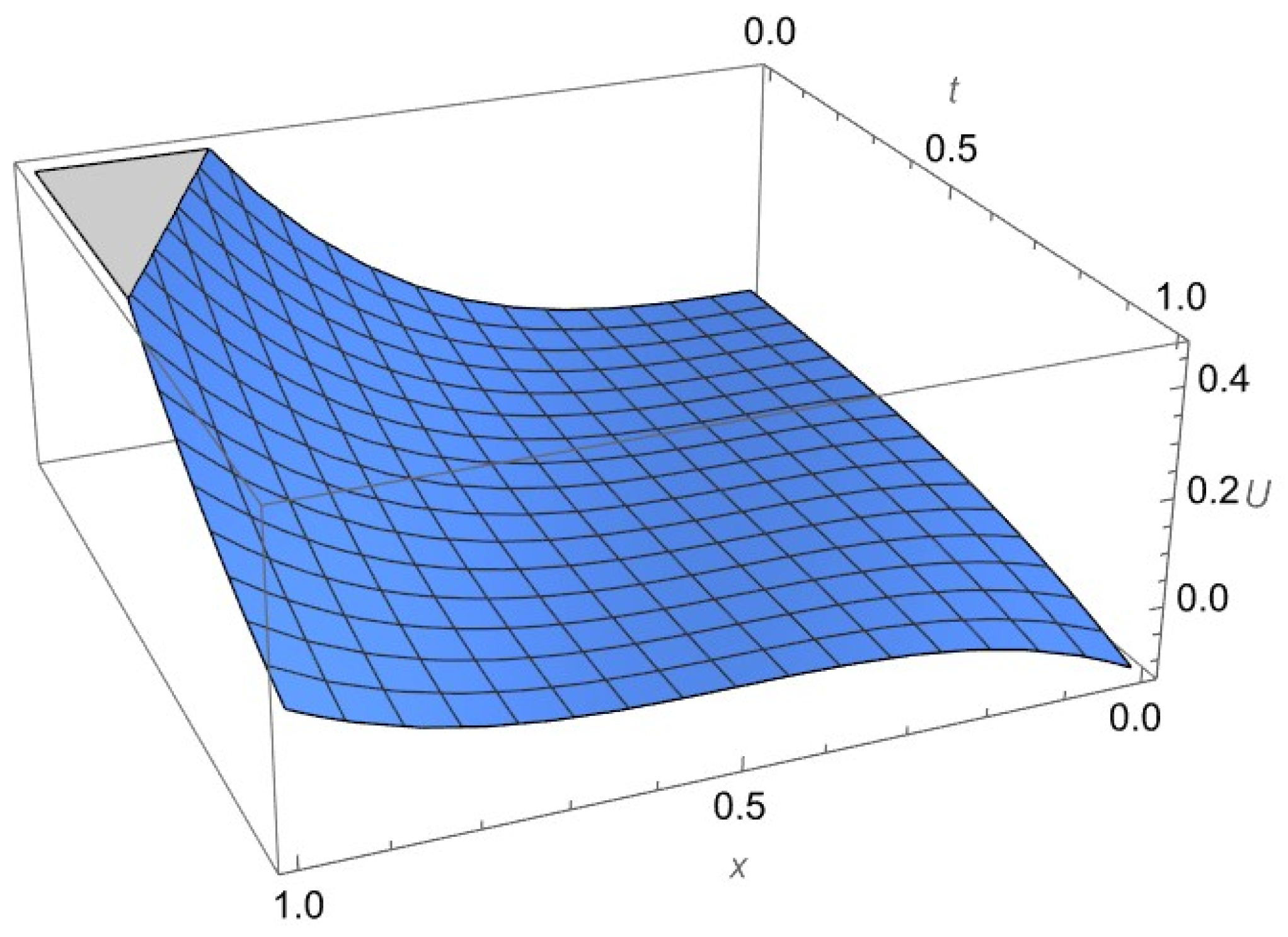
Figure 1. The approximate 3D solution, U(x), and the exact solution are depicted in Figure 1. This visual simulation highlights the significant overlap between the two solutions.
Axioms 13 00833 g001
Figure 2. The picture above presents the absolute error between the exact and approximate solutions. Notably, the absolute error is on the order of 10−16, indicating an extremely high degree of accuracy in the approximation. This level of precision suggests that the approximate solution closely aligns with the exact solution, making it a reliable choice for further analysis or applications.
Axioms 13 00833 g002
Figure 3. The approximate 3D solution U   ( x ,   t ) and the exact solution are shown in Figure 3, demonstrating that both solutions overlap.
Axioms 13 00833 g003
Figure 4. The absolute error between the exact and approximate solutions is displayed. The absolute error is of the order of 10 9 .
Axioms 13 00833 g004
Figure 5. The approximate 3D solution U   ( x ,   t ) and the exact solution are shown in Figure 5, demonstrating that both solutions overlap.
Axioms 13 00833 g005
Figure 6. The absolute error between the exact and approximate solutions is displayed in the picture. The absolute error is of the order of 10 16 .
Axioms 13 00833 g006
Figure 7. The approximate solution U   ( x ,   t ) and the exact solution are plotted in Figure 7. The graph shows that both solutions overlap.
Axioms 13 00833 g007
Figure 8. In the picture, the absolute error between the exact and approximate solutions is displayed. The absolute error is of the order of 10 7 .
Axioms 13 00833 g008
Figure 9. The approximate solution U   ( x ,   t ) and the exact solution are simulated in the figure, demonstrating that both solutions overlap very well with using only 10 B-polys.
Axioms 13 00833 g009
Figure 10. The absolute error between the exact and approximate solutions is displayed. The absolute error is of the order of 10 7  with only 10 B-polys used in the calculations.
Axioms 13 00833 g010
Table 1. Comparison of the proposed approach to the exact solution for Example 1. The solution at t = 0.5 and for various values of x is presented in the table.
Value of xValue of tApproximate Value of U (x, t) Using Current MethodExact Value of U (x, t)
0 0.5 0.015625 −0.015625
0.2 0.5 0.000125 −0.000125
0.4 0.5 0.003375 0.003375
0.6 0.5 0.042875 0.421875
0.8 0.5 0.166375 0.166375
1 0.5 0.421875 0.421875
Table 2. Comparison of the proposed approach to the exact solution for Example 1. The solution at t = 1.0 and for various values of x is presented in the table.
Value of xValue of tApproximate Value of U (x, t) Using Current MethodExact Value of U (x, t)
01 0.125000 0.125000
0.2 1 0.026999 0.026999
0.4 1 0.001000 0.001000
0.6 1 0.001000 0.001000
0.8 1 0.027000 0.027000
11 0.125000 0.125000
Table 3. Comparison of the proposed approach to the exact solution for Example 2. The solution at t = 0.5 and for various values of x is presented in the table.
Value of xValue of tApproximate Value of U (x, t) Using Current MethodExact Value of U (x, t)
0 0.5 0.247403 0.247403
0.2 0.5 0.049979 0.049979
0.4 0.5 0.149438 0.149438
0.6 0.5 0.342898 0.342898
0.8 0.5 0.522687 0.522687
1 0.5 0.681639 0.681639
Table 4. Comparison of the proposed approach to the exact solution for Example 2. The solution at t = 1.0 and for various values of x is presented in the table.
Value of xValue of tApproximate Value of U (x, t) Using Current MethodExact Value of U (x, t)
01 0.479424 0.479425
0.2 1 0.295520 0.295520
0.4 1 0.099833 0.099833
0.6 1 0.099833 0.099833
0.8 1 0.295520 0.295520
11 0.479425 0.479425
Table 5. Comparison of the proposed approach to the exact solution for Example 3. The solution at t = 0.5 and for various values of x is presented in the table.
Value of xValue of tApproximate Value of U (x, t) Using Current MethodExact Value of U (x, t)
0 0.5 0.250000 0.250000
0.2 0.5 0.406000 0.406000
0.4 0.5 0.738000 0.738000
0.6 0.5 1.342000 1.342000
0.8 0.5 2.314000 2.314000
1 0.5 3.750000 3.750000
Table 6. Comparison of the proposed approach to the exact solution for Example 3. The solution at t = 1.0 and for various values of x is presented in the table.
Value of xValue of tApproximate Value of U (x, t) Using Current MethodExact Value of U (x, t)
01 1.000000 1.000000
0.2 1 1.872000 1.872000
0.4 1 3.016000 3.016000
0.6 1 4.624000 4.624000
0.8 1 6.888000 6.888000
11 10.000000 10.000000
Table 7. Comparison of the proposed approach to the exact solution for Example 4 is presented. The solution at t = 0.5 and for various values of x is presented on the table.
Value of xValue of tApproximate Value of U (x, t) Using Current MethodExact Value of U (x, t)
0 0.5 1.615146 1.615146
0.2 0.5 1.681062 1.681062
0.4 0.5 1.895392 1.895392
0.6 0.5 2.315037 2.315037
0.8 0.5 3.063094 3.063094
1 0.5 4.390423 4.390423
Table 8. Comparison of the proposed approach to the exact solution for Example 4 and the solution at t = 1.0 and for various values of x is presented in the table.
Value of xValue of tApproximate Value of U (x, t) Using Current MethodExact Value of U (x, t)
01 2.319777 2.319777
0.2 1 2.414449 2.414449
0.4 1 2.722283 2.722283
0.6 1 3.325004 3.325004
0.8 1 4.399412 4.399412
11 6.305807 6.305807
Table 9. A comparison of the proposed approach to the exact solution for Example 5 is presented. The solution at t = 0.5 and for various values of x is presented in the table.
Value of xValue of tApproximate Value of U (x, t) Using Current MethodExact Value of U (x, t)
0 0.50.6065310.606531
0.2 0.50.6312840.631284
0.4 0.50.7117700.711770
0.6 0.50.8693580.869358
0.8 0.5 1.150274 1.150274
1 0.5 1.648721 1.648721
Table 10. A comparison of the proposed approach to the exact solution for Example 5 is presented. The solution at t = 1.0 and for various values of x is presented in the table.
Value of xValue of tApproximate Value of U (x, t) Using Current MethodExact Value of U (x, t)
0 1 0.367879 0.367879
0.2 1 0.382893 0.382893
0.4 1 0.431711 0.431711
0.6 1 0.527292 0.527292
0.8 1 0.697676 0.697676
1 1 1.000000 1.000000
Disclaimer/Publisher’s Note: The statements, opinions and data contained in all publications are solely those of the individual author(s) and contributor(s) and not of MDPI and/or the editor(s). MDPI and/or the editor(s) disclaim responsibility for any injury to people or property resulting from any ideas, methods, instructions or products referred to in the content.