Szász–Durrmeyer Operators Involving Confluent Appell Polynomials

Abstract

This article is concerned with the Durrmeyer-type generalization of Szász operators, including confluent Appell polynomials and their approximation properties. Also, the rate of convergence of the confluent Durrmeyer operators is found by using the modulus of continuity and Peetre’s $\mathcal{K}$-functional. Then, we show that, under special choices of $A\left(t\right)$, the newly constructed operators reduce confluent Hermite polynomials and confluent Bernoulli polynomials, respectively. Finally, we present a comparison of newly constructed operators with the Durrmeyer-type Szász operators graphically.

1. Introduction

As a polynomial set, an Appell set [1] satisfies the following criteria: the determining function that enables us to have

$$\mathit{A}\left(t\right)e^{xt}=\sum _{k=0}^{\infty }{P}_k\left(x\right)\frac{t^k}{k!}$$

(1)

is an official power series as follows:

$$A\left(t\right)=\sum _{k=0}^{\infty }{\theta }_k\frac{t^k}{k!},\left(A\left(0\right)\ne 0\right).$$

For some $r>0$, it is presumed that the series in (1) convergent in $\left|t\right|<r$. Another way to describe the Appell polynomials is the $P_k^{\prime }\left(x\right)=k{P}_{k-1}\left(x\right)$ recurrence formulas, where $k=1,2,\dots$.

Theorem 1.

Consider the polynomial sequence ${\left\{P_k^{\left(a,b\right)}\left(x\right)\right\}}_{k\ge 0}$, with $b\notin \left\{\dots ,-1,0\right\}$. Consequently, the ensuing statements are interchangeable.

(i) 

${\left\{P_k^{\left(a,b\right)}\left(x\right)\right\}}_{k\ge 0}$ is a confluent sequence of Appell polynomials.

(ii) 

${\left\{P_k^{\left(a,b\right)}\left(x\right)\right\}}_{k\ge 0}$’s generating function is granted by

$$\sum _{k=0}^{\infty }{P}_k^{\left(a,b\right)}\left(x\right)\frac{t^k}{k!}=A\left(t\right){}_{1}F_1\left(a;b;xt\right),$$

(2)

• where $\left\{{\theta }_k\right\}$ is unrelated to n with ${\theta }_0\ne 0$, an analytic function, $A\left(t\right)$ has an extension of power series

  $$A\left(t\right)=\sum _{k=0}^{\infty }{\theta }_k\frac{t^k}{k!},$$

  (3)
• and is an analytical function, and

  $${}_{1}F_1\left(a;b;z\right)=\sum _{k=0}^{\infty }\frac{{\left(a\right)}_k}{{\left(b\right)}_k}\frac{z^k}{k!}$$

  (4)
• is a confluent hypergeometric function. For all finite z, this function converges, assuming $b\notin \left\{\dots ,-1,0\right\}$ [2]. Then,

  $$\left\{\begin{array}{c}{\left(a\right)}_k=a\left(a+1\right)\dots \left(a+k-1\right);k\ge 1\hfill \\ {\left(a\right)}_0=1;1\hfill \end{array}\right.$$
• gives the definition of the Pocchammer symbol [2].

Jakimovski and Leviatan [3] construct the operators as follows

$$J_{\eta }\left(f;x\right)=\frac{e^{-\eta x}}{A\left(1\right)}\sum _{k=0}^{\infty }{P}_k\left(\eta x\right)f\left(\frac{k}{\eta }\right).$$

Mazhar and Totik [4] define Durrmeyer-type Szász operators as follows:

$$Z_{\eta }\left(f;x\right)=\eta \sum _{k=0}^{\infty }{e}^{-\eta x}\frac{{\left(\eta x\right)}^k}{k!}{\int }_0^{\infty }{e}^{-\eta t}\frac{{\left(\eta t\right)}^k}{k!}f\left(\frac{k}{\eta }\right).$$

Recently, Özarslan and Çekim [5] define confluent Jakimovski–Leviatan operators as

$$L_{\eta }\left(f;x\right)=\frac{1}{A\left(1\right){}_{1}F_1\left(a;b;\eta x\right)}\sum _{k=0}^{\infty }\frac{P_k^{\left(a,b\right)}\left(\eta x\right)}{k!}f\left(\frac{k}{\eta }\right),b>a>0$$

$\eta \in \mathbb{N}$ and $x\ge 0$.

Furthermore, it is expected that these operators fulfill the following requirements:

i.

$0\le \frac{{\theta }_k}{A\left(1\right)},k=0,1,\dots ,$ and $A\left(1\right)\ne 0$.

ii.

The series at (2) and (3) converge for $\left|t\right|<r\left(r>1\right)$.

Recently, they have remarkable studies in operator theory [6,7,8,9], analytic function theory [10], and other fields [11,12].

Now, we define the Durrmeyer-type generalization of Szász operators involving confluent Appell polynomials

$$S_{\eta }\left(f;x\right)=\frac{\eta }{\mathit{A}\left(1\right){}_{1}F_1\left(a;b;\eta x\right)}\sum _{k=0}^{\infty }\frac{P_k^{\left(a,b\right)}\left(\eta x\right)}{k!}{\int }_0^{\infty }{e}^{-\eta t}\frac{{\left(\eta t\right)}^k}{k!}f\left(t\right)dt,b>a>0$$

$P_k^{\left(a,b\right)}$ is given in (2), and $x\ge 0$, $\eta \in \mathbb{N}$.

2. Approximation Properties

In this section, we give moments and central moments for our operator including confluent Appell polynomials.

Lemma 1.

For any $x\in [0,\infty )$, we obtain

$$\begin{array}{ccc}\hfill S_{\eta }\left(1;x\right)& =& 1,\hfill \\ \hfill S_{\eta }\left(t;x\right)& =& \frac{{\left(a\right)}_1}{{\left(b\right)}_1}\frac{{}_{1}F_1\left(a+1;b+1;\eta x\right)}{{}_{1}F_1\left(a;b;\eta x\right)}x+\frac{A^{\prime }\left(1\right)}{\eta A\left(1\right)}+\frac{1}{\eta },\hfill \\ \hfill S_{\eta }\left(t^2;x\right)& =& \frac{{\left(a\right)}_2}{{\left(b\right)}_2}\frac{{}_{1}F_1\left(a+2;b+2;\eta x\right)}{{}_{1}F_1\left(a;b;\eta x\right)}{x}^2+\frac{{\left(a\right)}_1}{{\left(b\right)}_1}\frac{1}{\eta }\left(\frac{2A^{\prime }\left(1\right)}{A\left(1\right)}+3\right)\frac{{}_{1}F_1\left(a+1;b+1;\eta x\right)}{{}_{1}F_1\left(a;b;\eta x\right)}x\hfill \\ & & +\frac{A^{″}\left(1\right)+3A^{\prime }\left(1\right)}{{\eta }^{2}A\left(1\right)}+\frac{2}{{\eta }^2}.\hfill \end{array}$$

Proof. 

One way to illustrate the proof is to use it as given in (2)

$$\begin{array}{ccc}\hfill \sum _{k=0}^{\infty }\frac{P_k^{\left(a,b\right)}\left(\eta x\right)}{k!}& =& A\left(1\right){}_{1}F_1\left(a;b;\eta x\right),\hfill \\ \hfill \sum _{k=0}^{\infty }\frac{P_{k+1}^{\left(a,b\right)}\left(\eta x\right)}{k!}& =& A^{\prime }\left(1\right){}_{1}F_1\left(a;b;\eta x\right)+\frac{{\left(a\right)}_1}{{\left(b\right)}_1}\eta xA\left(1\right){}_{1}F_1\left(a+1;b+1;\eta x\right),\hfill \\ \hfill \sum _{k=0}^{\infty }\frac{P_{k+2}^{\left(a,b\right)}\left(\eta x\right)}{k!}& =& A^{″}\left(1\right){}_{1}F_1\left(a;b;\eta x\right)+A^{\prime }\left(1\right){}_{1}F_1\left(a;b;\eta x\right)+2\frac{{\left(a\right)}_1}{{\left(b\right)}_1}\eta x{A}^{\prime }\left(1\right){}_{1}F_1\left(a+1;b+1;\eta x\right)\hfill \\ & & +\frac{{\left(a\right)}_2}{{\left(b\right)}_2}{\left(\eta x\right)}^{2}A\left(1\right){}_{1}F_1\left(a+2;b+2;\eta x\right).\hfill \end{array}$$

By using these equalities in the operator, we obtain the desired results. □

Theorem 2.

For $f\in C[0,\infty )$,

$$\underset{n\to \infty }{lim}{S}_{\eta }\left(f;x\right)=f\left(x\right)$$

uniformly converges in every compact subset of $[0,\infty )$.

Proof. 

From (4) and Lemma 1, we obtain

$$\underset{\eta \to \infty }{lim}{S}_{\eta }\left(e_i;x\right)=e_i\left(x\right),i=0,1,2.$$

So, from the well-known Korovkin theorem [13] the proof is completed. □

Lemma 2.

The first and second central moments for $S_{\eta }$ are given as follows:

$$\begin{array}{ccc}\hfill S_{\eta }\left(t-x;x\right)& =& \left(\frac{{\left(a\right)}_1}{{\left(b\right)}_1}\frac{{}_{1}F_1\left(a+1;b+1;\eta x\right)}{{}_{1}F_1\left(a;b;\eta x\right)}-1\right)x+\frac{A^{\prime }\left(1\right)}{\eta A\left(1\right)}+\frac{1}{\eta },\hfill \\ \hfill S_{\eta }\left({\left(t-x\right)}^2;x\right)& =& \left(\frac{{\left(a\right)}_2}{{\left(b\right)}_2}\frac{{}_{1}F_1\left(a+2;b+2;\eta x\right)}{{}_{1}F_1\left(a;b;\eta x\right)}-2\frac{{\left(a\right)}_1}{{\left(b\right)}_1}\frac{{}_{1}F_1\left(a+1;b+1;\eta x\right)}{{}_{1}F_1\left(a;b;\eta x\right)}+1\right)x^2\hfill \\ & & +\left(\frac{{\left(a\right)}_1}{{\left(b\right)}_1}\frac{1}{\eta }\left(\frac{2A^{\prime }\left(1\right)}{A\left(1\right)}+3\right)\frac{{}_{1}F_1\left(a+1;b+1;\eta x\right)}{{}_{1}F_1\left(a;b;\eta x\right)}-\frac{2}{\eta }\left(\frac{A^{\prime }\left(1\right)}{A\left(1\right)}+1\right)\right)x\hfill \\ & & +\frac{A^{″}\left(1\right)+3A^{\prime }\left(1\right)}{{\eta }^{2}A\left(1\right)}+\frac{2}{{\eta }^2}.\hfill \end{array}$$

Proof. 

From the linearity of the operator and Lemma 1,

$$\begin{array}{ccc}\hfill S_{\eta }\left(t-x;x\right)& =& S_{\eta }\left(e_1;x\right)-x{S}_{\eta }\left(e_0;x\right),\hfill \\ \hfill S_{\eta }\left({\left(t-x\right)}^2;x\right)& =& S_{\eta }\left(e_2;x\right)-2x{S}_{\eta }\left(e_1;x\right)+x^2{S}_{\eta }\left(e_0;x\right).\hfill \end{array}$$

By using these equalities, the proof is completed. □

3. Rate of Convergence

In this section, we give the rate of convergence by the modulus of continuity, Peetre’s-$\mathcal{K}$ functional, and the second modulus of continuity, respectively. The modulus of continuity is given by

$$\omega \left(f,\delta \right):=\underset{\left|t-x\right|\le \delta }{sup}\underset{x\in [0,\infty )}{sup}\left|f\left(t\right)-f\left(x\right)\right|,\delta >0,$$

where $f\in C[0,\infty )$. It is due to the following feature of the modulus of continuity

$$\left|f\left(t\right)-f\left(x\right)\right|\le \left(1+\frac{\left|t-x\right|}{\delta }\right)\omega \left(f,\delta \right).$$

Theorem 3.

For every $x\in [0,\infty )$ and $f\in C[0,\infty )$,

$$\left|S_{\eta }\left(f;x\right)-f\left(x\right)\right|\le 2\omega \left(f,{\delta }_{\eta }\right),$$

where

$$\begin{array}{ccc}\hfill {\delta }_{\eta }\left(x\right)& =& \left\{\left(\frac{{\left(a\right)}_2}{{\left(b\right)}_2}\frac{{}_{1}F_1\left(a+2;b+2;\eta x\right)}{{}_{1}F_1\left(a;b;\eta x\right)}-2\frac{{\left(a\right)}_1}{{\left(b\right)}_1}\frac{{}_{1}F_1\left(a+1;b+1;\eta x\right)}{{}_{1}F_1\left(a;b;\eta x\right)}+1\right)x^2\right.\hfill \\ & & +\left(\frac{{\left(a\right)}_1}{{\left(b\right)}_1}\frac{1}{\eta }\left(\frac{2A^{\prime }\left(1\right)}{A\left(1\right)}+3\right)\frac{{}_{1}F_1\left(a+1;b+1;\eta x\right)}{{}_{1}F_1\left(a;b;\eta x\right)}-\frac{2}{\eta }\left(\frac{A^{\prime }\left(1\right)}{A\left(1\right)}+1\right)\right)x\hfill \\ & & {\left.+\frac{A^{″}\left(1\right)+3A^{\prime }\left(1\right)}{{\eta }^{2}A\left(1\right)}+\frac{2}{{\eta }^2}\right\}}^{\frac{1}{2}}.\hfill \end{array}$$

(5)

Proof. 

Using the operators $S_{\eta }$’s linearity and from Lemma 2, we obtain

$$\begin{array}{ccc}\hfill \left|S_{\eta }\left(f;x\right)-f\left(x\right)\right|& \le & \frac{\eta }{A\left(1\right){}_{1}F_1\left(a;b;\eta x\right)}\sum _{k=0}^{\infty }\frac{P_k^{\left(a,b\right)}\left(\eta x\right)}{k!}{\int }_0^{\infty }{e}^{-\eta t}\frac{{\left(\eta t\right)}^k}{k!}\left|f\left(t\right)-f\left(x\right)\right|dt\hfill \\ & & \le \frac{\eta }{A\left(1\right){}_{1}F_1\left(a;b;\eta x\right)}\sum _{k=0}^{\infty }\frac{P_k^{\left(a,b\right)}\left(\eta x\right)}{k!}{\int }_0^{\infty }{e}^{-\eta t}\frac{{\left(\eta t\right)}^k}{k!}\left(1+\frac{\left|t-x\right|}{\delta }\right)\omega \left(f,\delta \right)dt\hfill \\ & & \le \left\{1+\frac{\eta }{A\left(1\right){}_{1}F_1\left(a;b;\eta x\right)}\frac{1}{\delta }\sum _{k=0}^{\infty }\frac{P_k^{\left(a,b\right)}\left(\eta x\right)}{k!}{\int }_0^{\infty }{e}^{-\eta t}\frac{{\left(\eta t\right)}^k}{k!}\left|t-x\right|dt\right\}\omega \left(f,\delta \right).\hfill \end{array}$$

(6)

For integral by using the Cauchy–Schwarz inequality, it follows that

$$\begin{array}{ccc}\hfill \left|S_{\eta }\left(f;x\right)-f\left(x\right)\right|& \le & \left\{\left(\frac{\eta }{A\left(1\right){}_{1}F_1\left(a;b;\eta x\right)}+1\right)\frac{1}{\delta }\sum _{k=0}^{\infty }\frac{P_k^{\left(a,b\right)}\left(\eta x\right)}{k!}{\left({\int }_0^{\infty }{e}^{-\eta t}\frac{{\left(\eta t\right)}^k}{k!}dt\right)}^{\frac{1}{2}}\right.\hfill \\ & & \left.{\left({\int }_0^{\infty }{e}^{-\eta t}\frac{{\left(\eta t\right)}^k}{k!}{\left(t-x\right)}^{2}dt\right)}^{\frac{1}{2}}\right\}\omega \left(f,\delta \right).\hfill \\ \hfill \end{array}$$

Examining Cauchy–Schwarz disparity in summation, one can easily obtain

$$\begin{array}{ccc}\hfill \left|S_{\eta }\left(f;x\right)-f\left(x\right)\right|& \le & \left\{1+\frac{1}{\delta }{\left(\frac{\eta }{A\left(1\right){}_{1}F_1\left(a;b;\eta x\right)}\sum _{k=0}^{\infty }\frac{P_k^{\left(a,b\right)}\left(\eta x\right)}{k!}{\int }_0^{\infty }{e}^{-\eta t}\frac{{\left(\eta t\right)}^k}{k!}dt\right)}^{\frac{1}{2}}\right.\hfill \\ & & \left.\times {\left(\frac{\eta }{A\left(1\right){}_{1}F_1\left(a;b;\eta x\right)}\sum _{k=0}^{\infty }\frac{P_k^{\left(a,b\right)}\left(\eta x\right)}{k!}{\int }_0^{\infty }{e}^{-\eta t}\frac{{\left(\eta t\right)}^k}{k!}{\left(t-x\right)}^{2}dt\right)}^{\frac{1}{2}}\right\}\omega \left(f,\delta \right),\hfill \\ & =& \left\{1+\frac{1}{\delta }{\left(S_{\eta }\left(1;x\right)\right)}^{\frac{1}{2}}{\left(S_{\eta }\left({\left(t-x\right)}^2;x\right)\right)}^{\frac{1}{2}}\right\}\omega \left(f,\delta \right),\hfill \\ & =& \left\{1+\frac{1}{\delta }{\left({\delta }_{\eta }\left(x\right)\right)}^{\frac{1}{2}}\right\}\omega \left(f,\delta \right)\hfill \end{array}$$

where ${\delta }_{\eta }\left(x\right)$ is given by (5).

$$\left|S_{\eta }\left(f;x\right)-f\left(x\right)\right|\le \left\{1+\frac{1}{\delta }\sqrt{{\delta }_{\eta }\left(x\right)}\right\}\omega \left(f,\delta \right)$$

can be obtained by considering this inequality in (6). If we choose $\delta =\sqrt{{\delta }_{\eta }\left(x\right)}$, we can obtain the desired result. □

Lemma 3.

For $x\in [0,\infty )$ and $f\in C_B[0,\infty )$, we have

$$\left|S_{\eta }\left(f;x\right)\right|\le ∥f∥.$$

Proof. 

For $S_{\eta }$, we obtain

$$\begin{array}{ccc}\hfill \left|S_{\eta }\left(f;x\right)\right|& =& \left|\frac{1}{A\left(1\right){}_{1}F_1\left(a;b;\eta x\right)}\sum _{k=0}^{\infty }\frac{P_k^{\left(a,b\right)}\left(\eta x\right)}{k!}{\int }_0^{\infty }{e}^{-\eta t}\frac{{\left(\eta t\right)}^k}{k!}f\left(t\right)dt\right|\hfill \\ & \le & \frac{1}{A\left(1\right){}_{1}F_1\left(a;b;\eta x\right)}\sum _{k=0}^{\infty }\frac{P_k^{\left(a,b\right)}\left(\eta x\right)}{k!}\left|{\int }_0^{\infty }{e}^{-\eta t}\frac{{\left(\eta t\right)}^k}{k!}f\left(t\right)dt\right|\hfill \\ & \le & \frac{1}{A\left(1\right){}_{1}F_1\left(a;b;\eta x\right)}\sum _{k=0}^{\infty }\frac{P_k^{\left(a,b\right)}\left(\eta x\right)}{k!}{\int }_0^{\infty }{e}^{-\eta t}\frac{{\left(\eta t\right)}^k}{k!}\left|f\left(t\right)\right|dt\hfill \\ & \le & ∥f∥S_{\eta }\left(1;x\right)\hfill \\ & \le & ∥f∥.\hfill \end{array}$$

□

$C_B^2[0,\infty )$ is the space of the functions f, for which f, $f^{\prime }$, and $f^{″}$ are continuous on $[0,\infty )$. The norm on the space $C_B^2[0,\infty )$ is given by [14]

$${∥g∥}_{C_B^2[0,\infty )}:={∥g∥}_{C_B[0,\infty )}+{∥g^{\prime }∥}_{C_B[0,\infty )}+{∥g^{″}∥}_{C_B[0,\infty )}.$$

Now, we define classical Peetre’s-$\mathcal{K}$ functional as follows:

$$\mathcal{K}\left(f,\lambda \right):=\underset{g\in C_B^2[0,\infty )}{inf}\left\{∥f-g∥+\lambda ∥g^{″}∥\right\}$$

where $\lambda >0$.

Theorem 4.

Let $x\in [0,\infty )$ and $f\in C_B[0,\infty )$. Then, we have for all $\eta \in \mathbb{N}$,

$$\left|S_{\eta }\left(f;x\right)-f\left(x\right)\right|\le 2\mathcal{K}\left(f;{\lambda }_{\eta }\left(x\right)\right),$$

where

$${\lambda }_{\eta }\left(x\right)=\left(\frac{A^{″}\left(1\right)+A^{\prime }\left(1\right)\left(3+2\eta \right)}{2{\eta }^{2}A\left(1\right)}+\frac{3\eta +2}{2{\eta }^2}\right).$$

Proof. 

For a given function $g\in C_B^2[0,\infty )$, we have the following Taylor expansion

$$g\left(t\right)=g\left(x\right)+(t-x)g^{\prime }\left(x\right)+{\int }_x^t(t-s)g^{″}\left(s\right)ds.$$

(7)

Applying $S_{\eta }$ operator to Equation (7), we obtain

$$\begin{array}{ccc}\hfill \left|S_{\eta }(g;x)-g\left(x\right)\right|& =& \left|S_{\eta }\left((t-x)g^{\prime }\left(x\right);x\right)\right|+\left|S_{\eta }\left({\int }_x^t(t-s)g^{″}\left(s\right)ds;x\right)\right|\hfill \\ & \le & \left|\right|g^{\prime }{\left|\right|}_{C_B[0,\infty )}\left|S_{\eta }\left(t-x;x\right)\right|+\left|\right|g^{″}{\left|\right|}_{C_B[0,\infty )}\left|S_{\eta }\left({\int }_x^t(t-s)ds;x\right)\right|\hfill \\ & \le & \left|\right|g^{\prime }{\left|\right|}_{C_B[0,\infty )}\left|S_{\eta }\left(t-x;x\right)\right|+\frac{1}{2}\left|\right|g^{″}{\left|\right|}_{C_B[0,\infty )}{S}_{\eta }\left({(t-x)}^2;x\right).\hfill \end{array}$$

So,

$$\left|S_{\eta }(g;x)-g\left(x\right)\right|\le {\lambda }_{\eta }{\left|\right|g\left|\right|}_{C_B^2[0,\infty )}.$$

Using the above inequality and Lemma 3, we obtain

$$\begin{array}{ccc}\hfill \left|S_{\eta }(f;x)-f\left(x\right)\right|& =& \left|S_{\eta }(f;x)-f\left(x\right)+S_{\eta }(g;x)-S_{\eta }(g;x)+g\left(x\right)-g\left(x\right)\right|\hfill \\ & \le & \left|\right|f-{g\left|\right|}_{C_B[0,\infty )}\left|S_{\eta }(1;x)\right|+\left|\right|f-{g\left|\right|}_{C_B[0,\infty )}+\left|S_{\eta }(g;x)-g\left(x\right)\right|\hfill \\ & \le & 2\left(\left|\right|f-{g\left|\right|}_{C_B[0,\infty )}+{\lambda }_{\eta }{\left|\right|g\left|\right|}_{C_B^2[0,\infty )}\right)\hfill \\ & \le & 2\mathcal{K}\left(f;{\lambda }_{\eta }\right).\hfill \end{array}$$

As a result,

$$|S_{\eta }(f;x)-f\left(x\right)|\le 2\mathcal{K}\left(f;{\lambda }_{\eta }\right).$$

(8)

Thus, the proof is completed. □

For $f\in C_B[0,\infty )$, the second modulus of continuity is explained by

$${\omega }_2\left(f,\delta \right)=\underset{0<t\le \delta }{sup}{∥f\left(.+2t\right)-2f\left(.+t\right)+f\left(.\right)∥}_{C_B[0,\infty )}.$$

The relationship between Peetre’s-$\mathcal{K}$ functional and the second modulus of continuity is given as follows:

$$\mathcal{K}\left(f;\delta \right)\le A\left({\omega }_2\left(f,\sqrt{\delta }\right)+min\left(1,\delta \right){∥f∥}_{C_B[0,\infty )}\right),$$

(9)

where the constant A is unaffected by the values of f and $\delta$ from [15]. From (8) and (9),

$$|S_{\eta }(f;x)-f\left(x\right)|\le 2A\left({\omega }_2\left(f,\sqrt{{\lambda }_{\eta }}\right)+min\left(1,{\lambda }_{\eta }\right){∥f∥}_{C_B[0,\infty )}\right).$$

4. Special Cases

In this section, we define Durrmeyer–Szász operators including confluent Bernoulli polynomials $S_{\eta }^{\mathcal{B}}$ and Durrmeyer–Szász operators including confluent Hermite polynomials $S_{\eta }^{\mathcal{H}}$ by selecting $A\left(t\right)=\frac{t}{e^t-1}$ and $A\left(t\right)=e^{-\frac{t^2}{2}}$ in (2), respectively.

4.1. Approximation Properties for $S_{\eta }^{\mathcal{B}}$

Choosing $A\left(t\right)=\frac{t}{e^t-1}$ in (2) we obtain ${\mathcal{B}}_k^{(a,b)}$. The confluent Bernoulli polynomials have

$$\frac{t}{e^t-1}{}_{1}F_1\left(a;b;xt\right)=\sum _{k=0}^{\infty }{\mathcal{B}}_k^{\left(a,b\right)}\left(x\right)\frac{t^k}{k!},\left|t\right|<\pi$$

as their generating function, where $b\notin \left\{\dots ,-1,0\right\}$.

The Szász–Durrmeyer operators including confluent Bernoulli polynomials are presented as

$$S_{\eta }^{\mathcal{B}}\left(f;x\right)=\frac{\eta \left(e-1\right)}{{}_{1}F_1\left(a;b;\eta x\right)}\sum _{k=0}^{\infty }\frac{{\mathcal{B}}_k^{\left(a,b\right)}\left(\eta x\right)}{k!}{\int }_0^{\infty }f\left(t\right)\frac{{\left(\eta t\right)}^k}{k!}{e}^{-\eta t}dt.$$

Now, we give moments, central moments, and modulus of continuity for our operator including confluent Bernoulli polynomials.

Lemma 4.

For $x\in [0,\infty )$, we have the moments for $S_{\eta }^{\mathcal{B}}$ as follows:

$$\begin{array}{ccc}\hfill S_{\eta }^{\mathcal{B}}\left(1;x\right)& =& 1,\hfill \\ \hfill S_{\eta }^{\mathcal{B}}\left(t;x\right)& =& \frac{{\left(a\right)}_1}{{\left(b\right)}_1}\frac{{}_{1}F_1\left(a+1;b+1;\eta x\right)}{{}_{1}F_1\left(a;b;\eta x\right)}x+\frac{e-2}{\eta \left(e-1\right)},\hfill \\ \hfill S_{\eta }^{\mathcal{B}}\left(t^2;x\right)& =& \frac{{\left(a\right)}_2}{{\left(b\right)}_2}\frac{{}_{1}F_1\left(a+2;b+2;\eta x\right)}{{}_{1}F_1\left(a;b;\eta x\right)}{x}^2+\frac{{\left(a\right)}_1}{{\left(b\right)}_1}\left(\frac{3e-5}{\eta \left(e-1\right)}\right)\frac{{}_{1}F_1\left(a+1;b+1;\eta x\right)}{{}_{1}F_1\left(a;b;\eta x\right)}x\hfill \\ & & +\frac{e^2-4e+5}{{\eta }^2{\left(e-1\right)}^2}.\hfill \end{array}$$

Lemma 5.

For every $x\in [0,\infty )$ and by Lemma 4, the following identities verify

$$\begin{array}{ccc}\hfill S_{\eta }^{\mathcal{B}}\left(t-x;x\right)& =& \left(\frac{{\left(a\right)}_1}{{\left(b\right)}_1}\frac{{}_{1}F_1\left(a+1;b+1;\eta x\right)}{{}_{1}F_1\left(a;b;\eta x\right)}-1\right)x+\frac{e-2}{\eta \left(e-1\right)},\hfill \\ \hfill S_{\eta }^{\mathcal{B}}\left({\left(t-x\right)}^2;x\right)& =& \left(\frac{{\left(a\right)}_2}{{\left(b\right)}_2}\frac{{}_{1}F_1\left(a+2;b+2;\eta x\right)}{{}_{1}F_1\left(a;b;\eta x\right)}-2\frac{{\left(a\right)}_1}{{\left(b\right)}_1}\frac{{}_{1}F_1\left(a+1;b+1;\eta x\right)}{{}_{1}F_1\left(a;b;\eta x\right)}+1\right)x^2\hfill \\ & & +\left(\frac{{\left(a\right)}_1}{{\left(b\right)}_1}\left(\frac{3e-5}{\eta \left(e-1\right)}\right)\frac{{}_{1}F_1\left(a+1;b+1;\eta x\right)}{{}_{1}F_1\left(a;b;\eta x\right)}+\frac{4-2e}{\eta \left(e-1\right)}\right)x+\frac{e^2-4e+5}{{\eta }^2{\left(e-1\right)}^2}.\hfill \end{array}$$

Theorem 5.

For every $x\in [0,\infty )$ and $f\in C[0,\infty )$,

$$\left|S_{\eta }^{\mathcal{B}}\left(f;x\right)-f\left(x\right)\right|\le 2\omega \left(f,{\lambda }_{\eta }\right).$$

Here,

$$\begin{array}{ccc}\hfill {\lambda }_{\eta }\left(x\right)& =& \left\{\left(\frac{{\left(a\right)}_2}{{\left(b\right)}_2}\frac{{}_{1}F_1\left(a+2;b+2;\eta x\right)}{{}_{1}F_1\left(a;b;\eta x\right)}-2\frac{{\left(a\right)}_1}{{\left(b\right)}_1}\frac{{}_{1}F_1\left(a+1;b+1;\eta x\right)}{{}_{1}F_1\left(a;b;\eta x\right)}+1\right)x^2\right.\hfill \\ & & {\left.+\left(\frac{{\left(a\right)}_1}{{\left(b\right)}_1}\left(\frac{3e-5}{\eta \left(e-1\right)}\right)\frac{{}_{1}F_1\left(a+1;b+1;\eta x\right)}{{}_{1}F_1\left(a;b;\eta x\right)}+\frac{4-2e}{\eta \left(e-1\right)}\right)x+\frac{e^2-4e+5}{{\eta }^2{\left(e-1\right)}^2}\right\}}^{\frac{1}{2}}.\hfill \end{array}$$

(10)

Proof. 

Using linearity of the operators $S_{\eta }^{\mathcal{B}}$, we obtain

$$\begin{array}{ccc}\hfill \left|S_{\eta }^{\mathcal{B}}\left(f;x\right)-f\left(x\right)\right|& \le & \frac{\eta \left(e-1\right)}{{}_{1}F_1\left(a;b;\eta x\right)}\sum _{k=0}^{\infty }\frac{{\mathcal{B}}_k^{\left(a,b\right)}\left(\eta x\right)}{k!}{\int }_0^{\infty }{e}^{-\eta t}\frac{{\left(\eta t\right)}^k}{k!}\left|f\left(t\right)-f\left(x\right)\right|dt\hfill \\ & & \le \frac{\eta \left(e-1\right)}{{}_{1}F_1\left(a;b;\eta x\right)}\sum _{k=0}^{\infty }\frac{{\mathcal{B}}_k^{\left(a,b\right)}\left(\eta x\right)}{k!}{\int }_0^{\infty }{e}^{-\eta t}\frac{{\left(\eta t\right)}^k}{k!}\left(1+\frac{\left|t-x\right|}{\delta }\right)\omega \left(f,\delta \right)dt\hfill \\ & & \le \left\{1+\frac{\eta \left(e-1\right)}{{}_{1}F_1\left(a;b;\eta x\right)}\frac{1}{\delta }\sum _{k=0}^{\infty }\frac{{\mathcal{B}}_k^{\left(a,b\right)}\left(\eta x\right)}{k!}{\int }_0^{\infty }{e}^{-\eta t}\frac{{\left(\eta t\right)}^k}{k!}\left|t-x\right|dt\right\}\omega \left(f,\delta \right).\hfill \end{array}$$

(11)

By applying the Cauchy–Schwarz inequality to the last integral, we obtain

$$\begin{array}{ccc}\hfill \left|S_{\eta }^{\mathcal{B}}\left(f;x\right)-f\left(x\right)\right|& \le & \left\{\left(\frac{\eta \left(e-1\right)}{{}_{1}F_1\left(a;b;\eta x\right)}+1\right)\frac{1}{\delta }\sum _{k=0}^{\infty }\frac{{\mathcal{B}}_k^{\left(a,b\right)}\left(\eta x\right)}{k!}{\left({\int }_0^{\infty }{e}^{-\eta t}\frac{{\left(\eta t\right)}^k}{k!}dt\right)}^{\frac{1}{2}}\right.\hfill \\ & & \left.{\left({\int }_0^{\infty }{e}^{-\eta t}\frac{{\left(\eta t\right)}^k}{k!}{\left(t-x\right)}^{2}dt\right)}^{\frac{1}{2}}\right\}\omega \left(f,\delta \right).\hfill \\ \hfill \end{array}$$

Considering Cauchy–Schwarz inequality for summation and from Lemma 5, one can easily obtain

$$\begin{array}{ccc}\hfill \left|S_{\eta }^{\mathcal{B}}\left(f;x\right)-f\left(x\right)\right|& \le & \left\{1+\frac{1}{\delta }{\left(\frac{\eta \left(e-1\right)}{{}_{1}F_1\left(a;b;\eta x\right)}\sum _{k=0}^{\infty }\frac{{\mathcal{B}}_k^{\left(a,b\right)}\left(\eta x\right)}{k!}{\int }_0^{\infty }{e}^{-\eta t}\frac{{\left(\eta t\right)}^k}{k!}dt\right)}^{\frac{1}{2}}\right.\hfill \\ & & \left.\times {\left(\frac{\eta \left(e-1\right)}{{}_{1}F_1\left(a;b;\eta x\right)}\sum _{k=0}^{\infty }\frac{{\mathcal{B}}_k^{\left(a,b\right)}\left(\eta x\right)}{k!}{\int }_0^{\infty }{\left(t-x\right)}^2{e}^{-\eta t}\frac{{\left(\eta t\right)}^k}{k!}dt\right)}^{\frac{1}{2}}\right\}\omega \left(f,\delta \right),\hfill \\ & =& \left\{1+\frac{1}{\delta }{\left(S_{\eta }^{\mathcal{B}}\left(1;x\right)\right)}^{\frac{1}{2}}{\left(S_{\eta }^{\mathcal{B}}\left({\left(t-x\right)}^2;x\right)\right)}^{\frac{1}{2}}\right\}\omega \left(f,\delta \right),\hfill \\ & =& \left\{1+\frac{1}{\delta }{\left({\lambda }_{\eta }\left(x\right)\right)}^{\frac{1}{2}}\right\}\omega \left(f,\delta \right)\hfill \end{array}$$

where ${\lambda }_{\eta }\left(x\right)$ is given by (10).

$$\left|S_{\eta }^{\mathcal{B}}\left(f;x\right)-f\left(x\right)\right|\le \left\{1+\frac{1}{\delta }\sqrt{{\lambda }_{\eta }\left(x\right)}\right\}\omega \left(f,\delta \right)$$

can be obtained by considering this inequality in (11). If we choose $\delta =\sqrt{{\lambda }_{\eta }\left(x\right)}$, we achieve the desired result. □

4.2. Approximation Properties for $S_{\eta }^{\mathcal{H}}$

Choosing $A\left(t\right)=e^{-\frac{t^2}{2}}$ in (2), then we obtain ${\mathcal{H}}_k^{(a,b)}$. The confluent Hermite polynomials have

$$e^{-\frac{t^2}{2}}{}_{1}F_1\left(a;b;xt\right)=\sum _{k=0}^{\infty }{\mathcal{H}}_k^{\left(a,b\right)}\left(x\right)\frac{t^k}{k!},$$

as their generating function, where $b\notin \left\{\dots ,-1,0\right\}$.

The Szász–Durrmeyer operators including confluent Hermite polynomials are shown as

$$S_{\eta }^{\mathcal{H}}\left(f;x\right)=\frac{\eta e^{\frac{1}{2}}}{{}_{1}F_1\left(a;b;\eta x\right)}\sum _{k=0}^{\infty }\frac{{\mathcal{H}}_k^{\left(a,b\right)}\left(\eta x\right)}{k!}{\int }_0^{\infty }{e}^{-\eta t}\frac{{\left(\eta t\right)}^k}{k!}f\left(t\right)dt.$$

Now, we give moments, central moments, and modulus of continuity for our operator including confluent Hermite polynomials.

Lemma 6.

For $x\in [0,\infty )$, we obtain the moments for $S_{\eta }^{\mathcal{H}}$ as follows:

$$\begin{array}{ccc}\hfill S_{\eta }^{\mathcal{H}}\left(1;x\right)& =& 1,\hfill \\ \hfill S_{\eta }^{\mathcal{H}}\left(t;x\right)& =& \frac{{\left(a\right)}_1}{{\left(b\right)}_1}\frac{{}_{1}F_1\left(a+1;b+1;\eta x\right)}{{}_{1}F_1\left(a;b;\eta x\right)}x,\hfill \\ \hfill S_{\eta }^{\mathcal{H}}\left(t^2;x\right)& =& \frac{{\left(a\right)}_2}{{\left(b\right)}_2}\frac{{}_{1}F_1\left(a+2;b+2;\eta x\right)}{{}_{1}F_1\left(a;b;\eta x\right)}{x}^2+\frac{{\left(a\right)}_1}{{\left(b\right)}_1}\frac{1}{\eta }\frac{{}_{1}F_1\left(a+1;b+1;\eta x\right)}{{}_{1}F_1\left(a;b;\eta x\right)}x-\frac{1}{{\eta }^2}.\hfill \end{array}$$

Lemma 7.

For every $x\in [0,\infty )$ and by Lemma 6, the following identities verify

$$\begin{array}{ccc}\hfill S_{\eta }^{\mathcal{H}}\left(t-x;x\right)& =& \left(\frac{{\left(a\right)}_1}{{\left(b\right)}_1}\frac{{}_{1}F_1\left(a+1;b+1;\eta x\right)}{{}_{1}F_1\left(a;b;\eta x\right)}-1\right)x,\hfill \\ \hfill S_{\eta }^{\mathcal{H}}\left({\left(t-x\right)}^2;x\right)& =& \left(\frac{{\left(a\right)}_2}{{\left(b\right)}_2}\frac{{}_{1}F_1\left(a+2;b+2;\eta x\right)}{{}_{1}F_1\left(a;b;\eta x\right)}-2\frac{{\left(a\right)}_1}{{\left(b\right)}_1}\frac{{}_{1}F_1\left(a+1;b+1;\eta x\right)}{{}_{1}F_1\left(a;b;\eta x\right)}+1\right)x^2\hfill \\ & & +\left(\frac{{\left(a\right)}_1}{{\left(b\right)}_1}\frac{1}{\eta }\frac{{}_{1}F_1\left(a+1;b+1;\eta x\right)}{{}_{1}F_1\left(a;b;\eta x\right)}\right)x-\frac{1}{{\eta }^2}.\hfill \end{array}$$

Theorem 6.

For every $x\in [0,\infty )$ and $f\in C[0,\infty )$,

$$\left|S_{\eta }^{\mathcal{H}}\left(f;x\right)-f\left(x\right)\right|\le 2\omega \left(f,{\gamma }_{\eta }\right),$$

where

$$\begin{array}{ccc}\hfill {\gamma }_{\eta }\left(x\right)& =& \left(\frac{{\left(a\right)}_2}{{\left(b\right)}_2}\frac{{}_{1}F_1\left(a+2;b+2;\eta x\right)}{{}_{1}F_1\left(a;b;\eta x\right)}-2\frac{{\left(a\right)}_1}{{\left(b\right)}_1}\frac{{}_{1}F_1\left(a+1;b+1;\eta x\right)}{{}_{1}F_1\left(a;b;\eta x\right)}+1\right)x^2\hfill \\ & & +\left(\frac{{\left(a\right)}_1}{{\left(b\right)}_1}\frac{1}{\eta }\frac{{}_{1}F_1\left(a+1;b+1;\eta x\right)}{{}_{1}F_1\left(a;b;\eta x\right)}\right)x-\frac{1}{{\eta }^2}.\hfill \end{array}$$

(12)

Proof. 

From the linearity of the operators $S_{\eta }^{\mathcal{H}}$, we obtain

$$\begin{array}{ccc}\hfill \left|S_{\eta }^{\mathcal{H}}\left(f;x\right)-f\left(x\right)\right|& \le & \frac{\eta e^{\frac{1}{2}}}{{}_{1}F_1\left(a;b;\eta x\right)}\sum _{k=0}^{\infty }\frac{{\mathcal{H}}_k^{\left(a,b\right)}\left(\eta x\right)}{k!}{\int }_0^{\infty }{e}^{-\eta t}\frac{{\left(\eta t\right)}^k}{k!}\left|f\left(t\right)-f\left(x\right)\right|dt\hfill \\ & \le & \frac{\eta e^{\frac{1}{2}}}{{}_{1}F_1\left(a;b;\eta x\right)}\sum _{k=0}^{\infty }\frac{{\mathcal{H}}_k^{\left(a,b\right)}\left(\eta x\right)}{k!}{\int }_0^{\infty }{e}^{-\eta t}\frac{{\left(\eta t\right)}^k}{k!}\left(1+\frac{\left|t-x\right|}{\delta }\right)\omega \left(f,\delta \right)dt\hfill \\ & \le & \left\{1+\frac{\eta e^{\frac{1}{2}}}{{}_{1}F_1\left(a;b;\eta x\right)}\frac{1}{\delta }\sum _{k=0}^{\infty }\frac{{\mathcal{H}}_k^{\left(a,b\right)}\left(\eta x\right)}{k!}{\int }_0^{\infty }\left|t-x\right|e^{-\eta t}\frac{{\left(\eta t\right)}^k}{k!}dt\right\}\omega \left(f,\delta \right).\hfill \\ \hfill \end{array}$$

(13)

For integration, we apply the Cauchy–Schwarz inequality and obtain

$$\begin{array}{ccc}\hfill \left|S_{\eta }^{\mathcal{H}}\left(f;x\right)-f\left(x\right)\right|& \le & \left\{1+\frac{\eta e^{\frac{1}{2}}}{{}_{1}F_1\left(a;b;\eta x\right)}\frac{1}{\delta }\sum _{k=0}^{\infty }\frac{{\mathcal{H}}_k^{\left(a,b\right)}\left(\eta x\right)}{k!}{\left({\int }_0^{\infty }{e}^{-\eta t}\frac{{\left(\eta t\right)}^k}{k!}dt\right)}^{\frac{1}{2}}\right.\hfill \\ & & \left.{\left({\int }_0^{\infty }{e}^{-\eta t}\frac{{\left(\eta t\right)}^k}{k!}{\left(t-x\right)}^{2}dt\right)}^{\frac{1}{2}}\right\}\omega \left(f,\delta \right).\hfill \\ \hfill \end{array}$$

Examining Cauchy–Schwarz disparity in summation and from Lemma 7, one can easily obtain

$$\begin{array}{ccc}\hfill \left|S_{\eta }^{\mathcal{H}}\left(f;x\right)-f\left(x\right)\right|& \le & \left\{1+\frac{1}{\delta }{\left(\frac{\eta e^{\frac{1}{2}}}{{}_{1}F_1\left(a;b;\eta x\right)}\sum _{k=0}^{\infty }\frac{{\mathcal{H}}_k^{\left(a,b\right)}\left(\eta x\right)}{k!}{\int }_0^{\infty }{e}^{-\eta t}\frac{{\left(\eta t\right)}^k}{k!}dt\right)}^{\frac{1}{2}}\right.\hfill \\ & & \left.\times {\left(\frac{\eta e^{\frac{1}{2}}}{{}_{1}F_1\left(a;b;\eta x\right)}\sum _{k=0}^{\infty }\frac{{\mathcal{H}}_k^{\left(a,b\right)}\left(\eta x\right)}{k!}{\int }_0^{\infty }{e}^{-\eta t}\frac{{\left(\eta t\right)}^k}{k!}{\left(t-x\right)}^{2}dt\right)}^{\frac{1}{2}}\right\}\omega \left(f,\delta \right),\hfill \\ & =& \left\{1+\frac{1}{\delta }{\left(S_{\eta }^{\mathcal{H}}\left(1;x\right)\right)}^{\frac{1}{2}}{\left(S_{\eta }^{\mathcal{H}}\left({\left(t-x\right)}^2;x\right)\right)}^{\frac{1}{2}}\right\}\omega \left(f,\delta \right),\hfill \\ & =& \left\{1+\frac{1}{\delta }{\left({\gamma }_{\eta }\left(x\right)\right)}^{\frac{1}{2}}\right\}\omega \left(f,\delta \right)\hfill \end{array}$$

where ${\gamma }_{\eta }\left(x\right)$ is given by (12).

$$\left|S_{\eta }^{\mathcal{H}}\left(f;x\right)-f\left(x\right)\right|\le \left\{1+\frac{1}{\delta }\sqrt{{\gamma }_{\eta }\left(x\right)}\right\}\omega \left(f,\delta \right)$$

can be obtained by considering this inequality in (13). If we choose $\delta =\sqrt{{\gamma }_{\eta }\left(x\right)}$, we obtain the desired result. □

5. Graphical Analysis

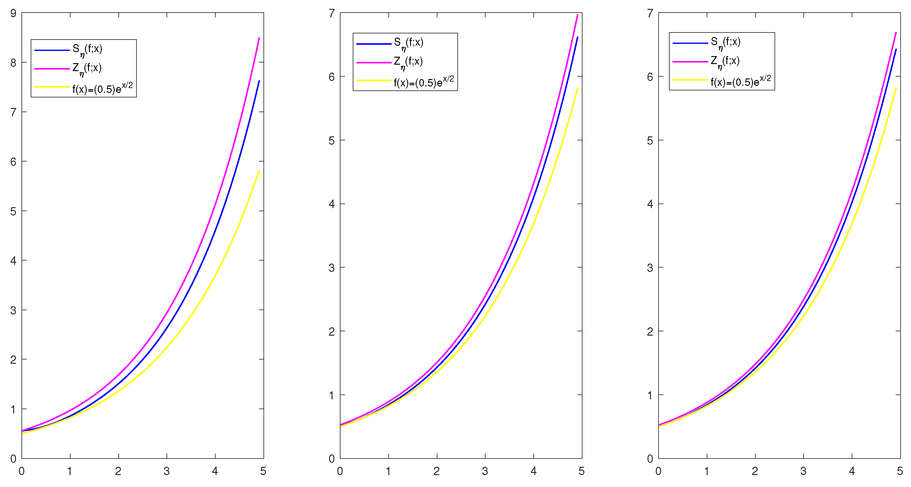
In this section, we will examine the approximations of both Durrmeyer-type Szász operators and the newly defined confluent Szász–Durrmeyer operators to a function f.

Let the function f be

$$f\left(x\right)=\left(0.5\right)exp\left(\frac{x}{2}\right).$$

Then, we plot the convergence of the newly constructed $S_{\eta }$ confluent Szász–Durrmeyer operators and $Z_{\eta }$ Durrmeyer-type Szász operators [4] to the function f in Figure 1 for $A\left(t\right)=1$. In Figure 1, we give three different illustrations for selected values $\left\{\eta =5,a=0.5,b=1.5\right\}$, $\left\{\eta =10,a=0.5,b=1.5\right\}$, and $\left\{\eta =12,a=1,b=2\right\}$, respectively.

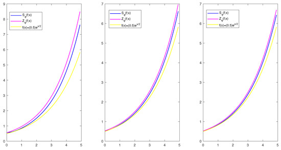
Figure 1. Illustration of approximation to the function $f\left(x\right)=\left(0.5\right)exp\left(\frac{x}{2}\right)$ for selected values $\left\{\eta =5,a=0.5,b=1.5\right\}$, $\left\{\eta =10,a=0.5,b=1.5\right\}$, and $\left\{\eta =12,a=1,b=2\right\}$, respectively.

By choosing $f\left(x\right)=\frac{log(x+1)}{1000}$, we show the error estimation of confluent Szász–Durrmeyer operators $S_{\eta }$ via the way of the modulus of continuity in Table 1.

Table 1. Error approximation for $S_{\eta }$ by using the modulus of continuity.

$\mathit{\eta }$	${\mathit{S}}_{\mathit{\eta }}\left(\mathit{f};\mathit{x}\right)$
10	0.00204334
${10}^2$	0.00138627
${10}^3$	0.00089236
${10}^4$	0.00054954
${10}^5$	0.00032734
${10}^6$	0.00019062
${10}^7$	0.00010942

6. Conclusions

In this study, Durrmeyer-type generalization of confluent Szász operators is constructed. The central moments of the newly constructed operators $S_{\eta }$ are obtained. Furthermore, the rate of convergence is investigated by using the modulus of continuity and Peetre’s $\mathcal{K}$-functional. The relationship between the newly constructed operators with ${\mathcal{B}}_k^{\left(a,b\right)}$ and ${\mathcal{H}}_k^{\left(a,b\right)}$ are given, respectively. Finally, the convergence of the confluent Szász–Durrmeyer operators $S_{\eta }$ and the classical Szász–Durrmeyer operators $Z_{\eta }$ to the selected functions are illustrated. The comparison of convergence is given by numerical examples.

References

- Appell, P. Sur une classe de polynomes. Ann. Sci. Ec. Norm. Suppl. 1880, 9, 119–144. [Google Scholar] [CrossRef]
- Rainville, E.D. Special Functions; The Macmillan Company: New York, NY, USA, 1960. [Google Scholar]
- Jakimovski, A.; Leviatan, D. Generalized Szász operators for the approximation in the finite interval. Mathematica 1969, 11, 97–103. [Google Scholar]
- Mazhar, S.; Totik, V. Approximation by modified Szász operators. Acta Sci. Math. 1985, 49, 257–269. [Google Scholar]
- Özarslan, M.A.; Çekim, B. Confluent Appell polynomials. J. Comput. Appl. Math. 2023, 424, 114984. [Google Scholar] [CrossRef]
- Liu, Y.J.; Cheng, W.T.; Zhang, W.H.; Ye, P.X. Approximation Properties of the Blending-Type Bernstein–Durrmeyer Operators. Axioms 2022, 12, 5. [Google Scholar] [CrossRef]
- El-Deeb, S.M.; Murugusundaramoorthy, G.; Vijaya, K.; Alburaikan, A. Pascu-Rønning Type Meromorphic Functions Based on Sălăgean-Erdély–Kober Operator. Axioms 2023, 12, 380. [Google Scholar] [CrossRef]
- Sabancıgil, P. Genuine q-Stancu-Bernstein–Durrmeyer Operators. Symmetry 2023, 15, 437. [Google Scholar] [CrossRef]
- Alotaibi, A. On the Approximation by Bivariate Szász–Jakimovski–Leviatan-Type Operators of Unbounded Sequences of Positive Numbers. Mathematics 2023, 11, 1009. [Google Scholar] [CrossRef]
- Khan, M.F.; Al-Shaikh, S.B.; Abubaker, A.A.; Matarneh, K. New Applications of Faber Polynomials and q-Fractional Calculus for a New Subclass of m-Fold Symmetric bi-Close-to-Convex Functions. Axioms 2023, 12, 600. [Google Scholar] [CrossRef]
- Chandragiri, S.; Shishkina, O.A. Generalized Bernoulli Numbers and Polynomials in the Context of the Clifford Analysis. J. Sib. Fed. Univ. Math. Phys. 2018, 11, 127–136. [Google Scholar]
- Leinartas, E.K.; Shishkina, O.A. The Discrete Analog of the Newton-Leibniz Formula in the Problem of Summation over Simplex Lattice Points. J. Sib. Fed. Univ. Math. Phys. 2019, 12, 503–508. [Google Scholar] [CrossRef]
- Korovkin, P.P. On convergence of linear operators in the space of continuous functions. Dokl. Akad. Nauk. SSSR 1953, 90, 961–964. (In Russian) [Google Scholar]
- Devore, R.A.; Lorentz, G.G. Constructive Approximation; Springer: Berlin, Germany, 1993. [Google Scholar]
- Ciupa, A. A class of integral Favard-Szász type operators. Stud. Univ. Babeş-Bolyai Math. 1995, 40, 39–47. [Google Scholar]
Disclaimer/Publisher’s Note: The statements, opinions and data contained in all publications are solely those of the individual author(s) and contributor(s) and not of MDPI and/or the editor(s). MDPI and/or the editor(s) disclaim responsibility for any injury to people or property resulting from any ideas, methods, instructions or products referred to in the content. |
© 2024 by the authors. Licensee MDPI, Basel, Switzerland. This article is an open access article distributed under the terms and conditions of the Creative Commons Attribution (CC BY) license (https://creativecommons.org/licenses/by/4.0/).