Regularization of the Boundary Equilibrium Bifurcation in Filippov System with Rich Discontinuity Boundaries

Abstract

This paper studies a particular type of planar Filippov system that consists of two discontinuity boundaries separating the phase plane into three disjoint regions with different dynamics. This type of system has wide applications in various subjects. As an illustration, a plant disease model and an avian-only model are presented, and their bifurcation scenarios are investigated. By means of the regularization approach, the blowing up method, and the singular perturbation theory, we provide a different way to analyze the dynamics of this type of Filippov system. In particular, the boundary equilibrium bifurcations of such systems are studied. As a consequence, the nonsmooth fold bifurcation becomes a saddle-node bifurcation, while the persistence bifurcation disappears after regularization.

1. Introduction

The Filippov system has been widely applied in many subjects, such as biology, electrical engineering, automatic control, and so on [1,2,3,4,5,6]. A Filippov system is a discontinuous dynamical system composed of two or more smooth vector fields that are separated by discontinuity boundaries [1,7]. In particular, the Filippov system consisting of one discontinuity boundary that separates the phase plane into two regions has been widely studied; see, for instance, [5,7,8,9,10]. There are also some analyses of the Filippov system with two discontinuity boundaries separating ${\mathbb{R}}^2$ into four regions; see [11,12,13,14]. Recently, some work on a Filippov system with two discontinuity boundaries separating ${\mathbb{R}}^2$ into three regions attracted our attention [15,16].

The case with three regions has fruitful applications in the real world. For example, such a Filippov plant disease model can help us understand disease transmission dynamics and provide economic and environmentally acceptable control strategies [15]. An avian-only model that incorporates culling off the infected and susceptible birds can also be described by a Filippov system with two discontinuity boundaries separating ${\mathbb{R}}^2$ into three regions [16].

The inspiration for this work is the work by Chen [15] and Yang [16], where the stability of different types of equilibria of such a Filippov system is studied. However, the bifurcation analysis of such systems is rare, particularly the boundary equilibrium bifurcation. In fact, boundary equilibrium bifurcations of Filippov systems have received more and more attention in the past decades [2,16,17,18,19,20]. In this work, we investigate the boundary equilibrium bifurcations of Filippov systems with two discontinuity boundaries. Instead of the classical Filippov convention, we choose the regularization method to study the dynamics of such systems, which enables us to build up a relationship between discontinuity-induced bifurcations and smooth bifurcations. The analysis of the present work shows that the equilibrium bifurcation either becomes a saddle-node bifurcation or disappears after regularization.

There are different ways to regularize a Filippov system [21,22,23,24,25,26,27]. In this work, we chose the method introduced by Sotomayor and Teixeira [27]. This method has already been applied to the case where the discontinuity boundary divides ${\mathbb{R}}^2$ into two regions [28,29,30,31,32,33,34,35,36] and into four regions [11,14,37]. However, according to the authors’ knowledge, they have not been applied to the case with three regions, which have more applications in reality.

In the process of regularization, the singular perturbation theory and blowing up technique play an important role. As we see in Section 3, the regularized system $R_Z$ can be reduced to a singular perturbation problem after a scaling transformation. The regularized system is characterized by two time scales, slow time t and fast time $\tau$, which are related by $\tau =t/\epsilon$. The slow-time system defines a reduced system for $\epsilon =0$ [28]. The dynamics of the singular perturbation problem are obtained by combining the two distinguished limits at $\epsilon =0$: the slow-time dynamics and the fast-time dynamics.

The structure of this paper is organized as follows: The next section is an overview of the Filippov system with rich discontinuity boundaries, different types of equilibria, the regularization method, and the geometric singular perturbation theory. Additionally, the definition of persistence bifurcation and nonsmooth fold bifurcation are given. In Section 3, we present the main results of this work. The bifurcation analysis of a Filippov plant disease model and its corresponding regularization are investigated in Section 3.1. The bifurcations and phase portraits of a Filippov avian-only model and its corresponding regularization are presented in Section 3.2. In Section 4, we summarize the main results of this paper and point out the future direction.

2. Preliminaries

The definition of a Filippov system that has rich boundaries, different types of equilibria, the regularization method, and two kinds of boundary equilibrium bifurcations is introduced in this section.

2.1. Definition of a Filippov System with Rich Boundaries

The planar Filippov system with one discontinuity boundary that separates ${\mathbb{R}}^2$ into two regions has been widely studied in much of the literature; see its definition, for instance, in [3,5,38,39]. In this paper, we study the planar Filippov system with two discontinuity boundaries that separates ${\mathbb{R}}^2$ into three regions, that is,

$$\begin{array}{c}\hfill Z\left(X\right)=\left\{\begin{array}{cc}{F}_1\left(X\right),\hfill & \mathrm{if}X\in G_1,\hfill \\ F_2\left(X\right),\hfill & \mathrm{if}X\in G_2,\hfill \\ F_3\left(X\right),\hfill & \mathrm{if}X\in G_3,\hfill \end{array}\right.\end{array}$$

(1)

where $X=(x,y)\in {\mathbb{R}}^2$. The vector fields $F_1,F_2,F_3$ are given by $F_1=(f_1,g_1),F_2=(f_2,g_2),F_3=(f_3,g_3)$. The discontinuity set $\mathsf{\Sigma }$ is composed of two parts:

$${\mathsf{\Sigma }}_1=\{X\in {\mathbb{R}}^2:H_1\left(X\right)=0\},{\mathsf{\Sigma }}_2=\{X\in {\mathbb{R}}^2:H_2\left(X\right)=0,H_1\left(X\right)\ge 0\},$$

where $H_1,H_2$ are smooth scalar functions. For instance, here, we consider $H_1\left(X\right)=y-y_0,H_2\left(X\right)=x-x_0$. The intersection of the discontinuity boundaries ${\mathsf{\Sigma }}_1$ and ${\mathsf{\Sigma }}_2$ is the point $(x_0,y_0)$. The boundaries separate ${\mathbb{R}}^2$ into three regions, $G_1$, $G_2$, and $G_3$, defined as

$$\begin{array}{cc}\hfill G_1& =\{X\in {\mathbb{R}}^2:H_1\left(X\right)<0\}=\{X\in {\mathbb{R}}^2:y<y_0\},\hfill \\ \hfill G_2& =\{X\in {\mathbb{R}}^2:H_1\left(X\right)>0,H_2\left(X\right)<0\}=\{X\in {\mathbb{R}}^2:y>y_0,x<x_0\},\hfill \\ \hfill G_3& =\{X\in {\mathbb{R}}^2:H_1\left(X\right)>0,H_2\left(X\right)>0\}=\{X\in {\mathbb{R}}^2:y>y_0,x>x_0\}.\hfill \end{array}$$

For convenience, we use the following notations in the subsequent discussion:

$$\begin{array}{ccc}\hfill & {\mathsf{\Sigma }}_{+,y_0}=\left\{(x,y_0)\right|x>x_0\},\hfill & {\mathsf{\Sigma }}_{-,y_0}=\left\{(x,y_0)\right|x<x_0\},\hfill \\ \hfill & {\mathsf{\Sigma }}_{x_0,+}=\left\{(x_0,y)\right|y>y_0\},\hfill & {\mathsf{\Sigma }}_{x_0,y_0}=\left\{(x_0,y_0)\right\}.\hfill \end{array}$$

Notice that ${\mathsf{\Sigma }}_1={\mathsf{\Sigma }}_{+,y_0}\cup {\mathsf{\Sigma }}_{-,y_0}\cup {\mathsf{\Sigma }}_{x_0,y_0}$ and ${\mathsf{\Sigma }}_2={\mathsf{\Sigma }}_{x_0,+}\cup {\mathsf{\Sigma }}_{x_0,y_0}$. The distribution of ${\mathbb{R}}^2$ by the discontinuity boundaries is presented in Figure 1.

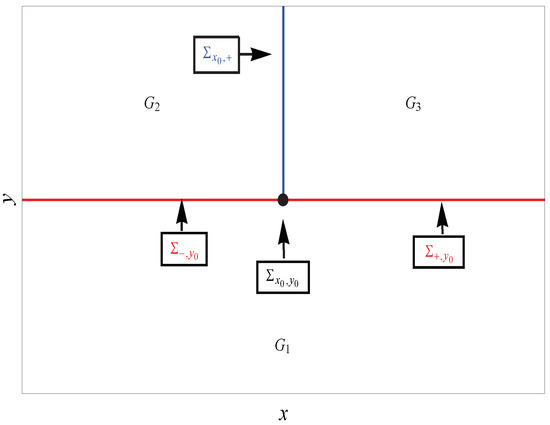
Figure 1. The discontinuity set separates ${\mathbb{R}}^2$ into three regions $G_1,G_2,G_3$.

With the above notations, $Z\left(X\right)$ can be rewritten as the general Filippov system $Z\left(X\right)=(Z_1\left(X\right),Z_2\left(X\right),Z_3\left(X\right))$, where

$$\begin{array}{c}\hfill Z_1\left(X\right)=\left\{\begin{array}{cc}{F}_1\left(X\right),\hfill & \mathrm{if}X\in G_1,\hfill \\ F_3\left(X\right),\hfill & \mathrm{if}X\in G_3,\hfill \end{array}\right.\end{array}$$

with the discontinuity boundary ${\mathsf{\Sigma }}_{+,y_0}$,

$$\begin{array}{c}\hfill Z_2\left(X\right)=\left\{\begin{array}{cc}{F}_1\left(X\right),\hfill & \mathrm{if}X\in G_1,\hfill \\ F_2\left(X\right),\hfill & \mathrm{if}X\in G_2,\hfill \end{array}\right.\end{array}$$

with the discontinuity boundary ${\mathsf{\Sigma }}_{-,y_0}$, and

$$\begin{array}{c}\hfill Z_3\left(X\right)=\left\{\begin{array}{cc}{F}_2\left(X\right),\hfill & \mathrm{if}X\in G_2,\hfill \\ F_3\left(X\right),\hfill & \mathrm{if}X\in G_3,\hfill \end{array}\right.\end{array}$$

with the discontinuity boundary ${\mathsf{\Sigma }}_{x_0,+}$. The dynamics of Z in $G_1$, $G_2$, and $G_3$ are defined by the flows of $F_1$, $F_2$, and $F_3$, respectively. The dynamics of the discontinuity boundaries are defined in the usual way. Here, we take the subsystem $Z_3$ as an example to define its dynamics when $X\in {\mathsf{\Sigma }}_{x_0,+}$. Following [1], the boundary ${\mathsf{\Sigma }}_{x_0,+}$ is divided into the following:

• The sliding region: ${\mathsf{\Sigma }}_{x_0,+}^s=\{X\in {\mathsf{\Sigma }}_{x_0,+}:\left(H_2{F}_2\left(X\right)\right)·\left(H_2{F}_3\left(X\right)\right)\le 0\}$,
• The crossing region: ${\mathsf{\Sigma }}_{x_0,+}^c=\{X\in {\mathsf{\Sigma }}_{x_0,+}:\left(H_2{F}_2\left(X\right)\right)·\left(H_2{F}_3\left(X\right)\right)>0\}$,

where $H_2{F}_i=\left({\displaystyle \frac{\partial H_2}{\partial x},\frac{\partial H_2}{\partial y}}\right)·(f_i,g_i),i=2,3$.

On the sliding region ${\mathsf{\Sigma }}_{x_0,+}^s$, the sliding vector field $F_{23}$ is defined by the Filippov’s convex method [7] as

$$F_{23}=(1-{\lambda }_{23})F_2+{\lambda }_{23}{F}_3,$$

(2)

where

$${\lambda }_{23}\left(X\right)=\frac{H_2{F}_2\left(X\right)}{H_2(F_2-F_3)\left(X\right)},0\le {\lambda }_{23}\le 1.$$

In a similar way, the sliding vector fields $F_{12}$ and $F_{13}$ are defined as

$$F_{12}=(1-{\lambda }_{12})F_1+{\lambda }_{12}{F}_2\mathrm{with}{\lambda }_{12}\left(X\right)=\frac{H_1{F}_1\left(X\right)}{H_1(F_1-F_2)\left(X\right)},$$

$$F_{13}=(1-{\lambda }_{13})F_1+{\lambda }_{13}{F}_3\mathrm{with}{\lambda }_{13}\left(X\right)=\frac{H_1{F}_1\left(X\right)}{H_1(F_1-F_3)\left(X\right)}.$$

2.2. Definition of Equilibria

This part distinguishes different types of equilibria in the Filippov system (1).

Definition 1 

(Admissible equilibrium). A point $X\in G=G_1\cup G_2\cup G_3$ is an admissible equilibrium of (1) if

$$F_i\left(X\right)=0,X\in G_i,$$

where $i=1,2,3$.

Definition 2 

(Pseudo-equilibrium). A point $\tilde{X}$ is a pseudoequilibrium of (1) if it is an equilibrium of the sliding vector fields $F_{12},F_{13}$, or $F_{23}$, i.e.,

$$F_{12}\left(\tilde{X}\right)=0,\tilde{X}\in {\mathsf{\Sigma }}_{-,y_0}^s,$$

or

$$F_{13}\left(\tilde{X}\right)=0,\tilde{X}\in {\mathsf{\Sigma }}_{+,y_0}^s,$$

or

$$F_{23}\left(\tilde{X}\right)=0,\tilde{X}\in {\mathsf{\Sigma }}_{x_0,+}^s.$$

Here, ${\mathsf{\Sigma }}_{-,y_0}^s,{\mathsf{\Sigma }}_{+,y_0}^s$ denote the sliding region on the boundary ${\mathsf{\Sigma }}_{-,y_0},{\mathsf{\Sigma }}_{+,y_0}$, respectively.

Definition 3 

(Boundary equilibrium). A point $\widehat{X}$ is termed as a boundary equilibrium of (1) on ${\mathsf{\Sigma }}_{-,y_0}$ if

$$\begin{array}{c}\hfill F_1\left(\widehat{X}\right)=0and{H}_1\left(\widehat{X}\right)=0,\\ \hfill or{F}_2\left(\widehat{X}\right)=0and{H}_1\left(\widehat{X}\right)=0;\end{array}$$

a boundary equilibrium on ${\mathsf{\Sigma }}_{+,y_0}$ if

$$\begin{array}{c}\hfill F_1\left(\widehat{X}\right)=0and{H}_1\left(\widehat{X}\right)=0,\\ \hfill or{F}_3\left(\widehat{X}\right)=0and{H}_1\left(\widehat{X}\right)=0;\end{array}$$

a boundary equilibrium on ${\mathsf{\Sigma }}_{x_0,+}$ if

$$\begin{array}{c}\hfill F_2\left(\widehat{X}\right)=0and{H}_2\left(\widehat{X}\right)=0,\\ \hfill or{F}_3\left(\widehat{X}\right)=0and{H}_2\left(\widehat{X}\right)=0.\end{array}$$

2.3. Description of the Regularization Method

The regularization method provides a different way to study the dynamics of Filippov systems. The regularization of a Filippov system is a smooth approximation of the Filippov system that removes the discontinuities. Therefore, the regularization makes it possible to construct a relationship between the Filippov systems and smooth systems.

In this section, we briefly review the regularization method proposed in [27]. It should be noticed that for system (1), the discontinuity boundary loses smoothness at the intersection point $(x_0,y_0)$. It needs additional blow-up before applying the regularization method, which is shown more detail in Section 3.

Definition 4. 

A $C^{\infty }$ function φ : $\mathbb{R}\to \mathbb{R}$ is a transition function if $\phi \left(x\right)=-1$ for $x\le -1$, $\phi \left(x\right)=1$ for $x\ge 1$ and ${\phi }^{\prime }\left(x\right)>0$ if $x\in (-1,1)$.

Given a Filippov system

$$\begin{array}{c}\hfill Z\left(X\right)=\left\{\begin{array}{cc}F\left(X\right),\hfill & ifH\left(X\right)<0,\hfill \\ G\left(X\right),\hfill & ifH\left(X\right)>0,\hfill \end{array}\right.\end{array}$$

(3)

where $H\left(X\right)$ is a smooth scalar function, and the discontinuity boundary is $\mathsf{\Sigma }=\{X\in {\mathbb{R}}^2:H\left(X\right)=0\}$, the regularization of (3) is a 1-parameter family given by

$$R_Z\left(X\right)=\left({\displaystyle \frac{1}{2}+\frac{{\phi }_{\epsilon }\left(H\left(X\right)\right)}{2}}\right)G\left(X\right)+\left({\displaystyle \frac{1}{2}-\frac{{\phi }_{\epsilon }\left(H\left(X\right)\right)}{2}}\right)F\left(X\right),$$

(4)

with ${\phi }_{\epsilon }\left(x\right)=\phi \left({\displaystyle \frac{x}{\epsilon }}\right)$ for $\epsilon >0$.

2.4. Geometric Singular Perturbation Theory

Geometric singular perturbation theory $\left(GSPT\right)$ is an important tool in the field of continuous dynamical systems. A singular perturbation problem in ${\mathbb{R}}^2$ is a differential system which can be written as

$$\begin{array}{ccc}\hfill & x^{\prime }=dx/d\tau =f(x,y,\epsilon ),\hfill & y^{\prime }=dy/d\tau =\epsilon g(x,y,\epsilon ),\hfill \end{array}$$

(5)

or equivalently, after the time rescaling $t=\epsilon \tau$,

$$\begin{array}{ccc}\hfill & \epsilon \dot{x}=dx/dt=f(x,y,\epsilon ),\hfill & \dot{y}=dy/dt=g(x,y,\epsilon ),\hfill \end{array}$$

(6)

where $(x,y)\in {\mathbb{R}}^2$, $f,g$ are smooth functions. Here, system (5) is called the fast system. System (6) is called the slow system. Observe that for $\epsilon >0$, the phase portraits of the fast and the slow systems coincide. When $\epsilon =0$, the set

$$\mathcal{M}=\left\{\right(x,y):f(x,y,0)=0\}$$

(7)

consists of all the equilibria of the fast system. We call $\mathcal{M}$ the slow manifold of the singular perturbation problem. A point $p\in \mathcal{M}$ is said to be normally hyperbolic if ${\left.{\displaystyle \frac{\partial f}{\partial x}}\right|}_p\ne 0$.

Notice that when $\epsilon =0$, the slow system defines a dynamical system on $\mathcal{M}$, called the reduced problem:

$$f(x,y,0)=0,\dot{y}=g(x,y,0).$$

(8)

Combining results on the dynamics of these two limiting problems, one obtains information on the dynamics for small values of $\epsilon$; more details are provided in [28].

2.5. Description of the Boundary Equilibrium Bifurcations

The two types of boundary equilibrium bifurcations discussed in this work are given here. More details about these bifurcations can be found in [1,20,40].

• Boundary Equilibrium Bifurcations:
  • Persistence:
    A branch of admissible equilibria firstly turns into a boundary equilibrium, and then a branch of pseudoequilibria as the parameter varies;
  • Nonsmooth fold bifurcation:
    A branch of admissible equilibria collides with a pseudoequilibrium, then becomes a boundary point, and then both disappear as the parameter varies.

3. Main Results and Examples

Since system (1) is composed of several parts of boundaries, that is, $\mathsf{\Sigma }={\mathsf{\Sigma }}_{+,y_0}\cup {\mathsf{\Sigma }}_{-,y_0}\cup {\mathsf{\Sigma }}_{x_0,+}\cup {\mathsf{\Sigma }}_{x_0,y_0}$, we have to apply the regularization method to each part separately. Notice that the boundaries lose smoothness at ${\mathsf{\Sigma }}_{x_0,y_0}$, or the point $(x_0,y_0)$, so this point needs additional consideration, which is explained by specific examples in the next section. Here, we only present the formula for regularizing system (1) at the boundaries ${\mathsf{\Sigma }}_{+,y_0}$, ${\mathsf{\Sigma }}_{-,y_0}$, and ${\mathsf{\Sigma }}_{x_0,+}$.

Recall that system (1) can be written as $Z\left(X\right)=(Z_1\left(X\right),Z_2\left(X\right),Z_3\left(X\right))$ with the boundaries ${\mathsf{\Sigma }}_{+,y_0}$, ${\mathsf{\Sigma }}_{-,y_0}$, ${\mathsf{\Sigma }}_{x_0,+}$. Next, we apply the regularization method in [27] to the subsystems $Z_1\left(X\right)$, $Z_2\left(X\right)$, and $Z_3\left(X\right)$.

• For the subsystem $Z_1$ with the boundary $y=y_0,x>x_0$, its regularization is given by

  $$R_{Z_1}=\left[{\displaystyle \frac{1}{2}+\frac{1}{2}\phi \left({\displaystyle \frac{y-y_0}{\epsilon }}\right)}\right]F_3(x,y)+\left[{\displaystyle \frac{1}{2}-\frac{1}{2}\phi \left({\displaystyle \frac{y-y_0}{\epsilon }}\right)}\right]F_1(x,y).$$

  (9)
• For $Z_2$ with the boundary $y=y_0,x<x_0$, its regularization is

  $$R_{Z_2}=\left[{\displaystyle \frac{1}{2}+\frac{1}{2}\phi \left({\displaystyle \frac{y-y_0}{\epsilon }}\right)}\right]F_2(x,y)+\left[{\displaystyle \frac{1}{2}-\frac{1}{2}\phi \left({\displaystyle \frac{y-y_0}{\epsilon }}\right)}\right]F_1(x,y).$$

  (10)
• For $Z_3$ with the boundary $x=x_0,y>y_0$, its regularization is

  $$R_{Z_3}=\left[{\displaystyle \frac{1}{2}+\frac{1}{2}\phi \left({\displaystyle \frac{x-x_0}{\epsilon }}\right)}\right]F_3(x,y)+\left[{\displaystyle \frac{1}{2}-\frac{1}{2}\phi \left({\displaystyle \frac{x-x_0}{\epsilon }}\right)}\right]F_2(x,y).$$

  (11)

For the subsystem $R_{Z_1}$, assuming $u=(y-y_0)/\epsilon$, system (9) can be written as a singular perturbation problem

$${\displaystyle \frac{d}{dt}\left(\begin{array}{c}x\\ \epsilon u\end{array}\right)=\left(\begin{array}{c}{\displaystyle \frac{1}{2}\left(f_1(x,y)+f_3(x,y)\right)+\frac{\phi \left(u\right)}{2}\left(f_3(x,y)-f_1(x,y)\right)}\\ {\displaystyle \frac{1}{2}\left(g_1(x,y)+g_3(x,y)\right)+\frac{\phi \left(u\right)}{2}\left(g_3(x,y)-g_1(x,y)\right)}\end{array}\right)}.$$

(12)

By rescaling time by $\tau =t/\epsilon$, system (12) becomes

$${\displaystyle \frac{d}{d\tau }\left(\begin{array}{c}x\\ u\end{array}\right)=\left(\begin{array}{c}\epsilon \left[{\displaystyle \frac{1}{2}(f_1(x,y)+f_3(x,y))+\frac{\phi \left(u\right)}{2}(f_3(x,y)-f_1(x,y))}\right]\\ {\displaystyle \frac{1}{2}(g_1(x,y)+g_3(x,y))+\frac{\phi \left(u\right)}{2}(g_3(x,y)-g_1(x,y))}\end{array}\right)}.$$

(13)

The slow manifold ${\mathcal{M}}_1$ is given by

$${\mathcal{M}}_1=\left\{{\displaystyle (u,y):\frac{1}{2}(g_1(x,y)+g_3(x,y))+\frac{\phi \left(u\right)}{2}(g_3(x,y)-g_1(x,y))=0}\right\}.$$

Then, the slow system (12) defines a dynamical system on ${\mathcal{M}}_1$

$$\left(\begin{array}{c}dx/dt\\ 0\end{array}\right)=\left(\begin{array}{c}{\displaystyle \frac{1}{2}(f_1(x,y)+f_3(x,y))+\frac{\phi \left(u\right)}{2}(f_3(x,y)-f_1(x,y))}\\ {\displaystyle \frac{1}{2}(g_1(x,y)+g_3(x,y))+\frac{\phi \left(u\right)}{2}(g_3(x,y)-g_1(x,y))}\end{array}\right).$$

In a similar way, we derive the slow manifold ${\mathcal{M}}_2$ for system $R_{Z_2}$

$${\mathcal{M}}_2=\left\{{\displaystyle (u,y):\frac{1}{2}(g_1(x,y)+g_2(x,y))+\frac{\phi \left(u\right)}{2}(g_2(x,y)-g_1(x,y))=0}\right\},$$

and the reduced problem

$$\left(\begin{array}{c}dx/dt\\ 0\end{array}\right)=\left(\begin{array}{c}{\displaystyle \frac{1}{2}(f_1(x,y)+f_2(x,y))+\frac{\phi \left(u\right)}{2}(f_2(x,y)-f_1(x,y))}\\ {\displaystyle \frac{1}{2}(g_1(x,y)+g_2(x,y))+\frac{\phi \left(u\right)}{2}(g_2(x,y)-g_1(x,y))}\end{array}\right).$$

For system (11), suppose $v=(x-x_0)/\epsilon$, then it becomes

$${\displaystyle \frac{d}{dt}\left(\begin{array}{c}\epsilon v\\ y\end{array}\right)=\left(\begin{array}{c}{\displaystyle \frac{1}{2}(f_2(x,y)+f_3(x,y))+\frac{\phi \left(v\right)}{2}(f_3(x,y)-f_2(x,y))}\\ {\displaystyle \frac{1}{2}(g_2(x,y)+g_3(x,y))+\frac{\phi \left(v\right)}{2}(g_3(x,y)-g_2(x,y))}\end{array}\right).}$$

(14)

Rescaling time by $\tau =t/\epsilon$, system (14) becomes

$${\displaystyle \frac{d}{d\tau }\left(\begin{array}{c}v\\ y\end{array}\right)=\left(\begin{array}{c}{\displaystyle \frac{1}{2}(f_2(x,y)+f_3(x,y))+\frac{\phi \left(v\right)}{2}(f_3(x,y)-f_2(x,y))}\\ \epsilon \left[{\displaystyle \frac{1}{2}(g_2(x,y)+g_3(x,y))+\frac{\phi \left(v\right)}{2}(g_3(x,y)-g_2(x,y))}\right]\end{array}\right).}$$

(15)

The slow manifold ${\mathcal{M}}_3$ is given by

$${\mathcal{M}}_3=\left\{{\displaystyle (v,y):\frac{1}{2}(f_2(x,y)+f_3(x,y))+\frac{\phi \left(v\right)}{2}(f_3(x,y)-f_2(x,y))=0}\right\}.$$

The reduced problem is

$$\left(\begin{array}{c}0\\ dy/dt\end{array}\right)=\left(\begin{array}{c}{\displaystyle \frac{1}{2}(f_2(x,y)+f_3(x,y))+\frac{\phi \left(v\right)}{2}(f_3(x,y)-f_2(x,y))}\\ {\displaystyle \frac{1}{2}(g_2(x,y)+g_3(x,y))+\frac{\phi \left(v\right)}{2}(g_3(x,y)-g_2(x,y))}\end{array}\right).$$

Comparing the singular perturbation problem with Filippov system (1), we have the following results.

Theorem 1 

([14]). For the Filippov system $Z_i\left(X\right)$ and its regularization $R_{Z_i}\left(X\right)$, the trajectories of $R_{Z_i}\left(X\right)$ are the solutions of a singular perturbation problem. The sliding region is homeomorphic to the slow manifold, and the sliding vector field $F_j$ is homeomorphic to the reduced problem on ${\mathcal{M}}_i$, $i=1,2,3,j=13,12,23$.

Subsequently, we take two specific examples to illustrate the regularization of the Filippov system with rich discontinuity boundaries.

3.1. The Filippov Plant Disease Model

Plant diseases are currently one of the major threats to crop production and the worldwide economy [41,42]. Many different measures have been implemented to control plant diseases, such as the use of chemicals [43], rogue infected trees [44], and the removal of infected branches [45]. In order to understand the disease transmission dynamics and provide economic and environmentally acceptable control strategies, many mathematical models have been constructed [46]. More recently, a Filippov plant disease model that incorporates cutting off infected branches and replanting susceptible trees has been built [15]. The model [15] is constructed based on the following regulations:

• When $y<y_0$, no control strategy is taken;
• When $y>y_0,x<x_0$, infected branches are cut off at a rate of $c_1>0$, and disease-free trees are replanted at a rate of $d>0$;
• When $y>y_0,x>x_0$, infected branches are removed at a rate of $c_2>0$,

which can be written as a Filippov system with two boundaries:

$$Z\left(X\right)=\left\{\begin{array}{cc}{F}_1\left(X\right),\hfill & \mathrm{if}X\in G_1,\hfill \\ F_2\left(X\right),\hfill & \mathrm{if}X\in G_2,\hfill \\ F_3\left(X\right),\hfill & \mathrm{if}X\in G_3,\hfill \end{array}\right.$$

(16a)

where

$$\begin{array}{cc}\hfill F_1(x,y)& =(ax-\beta xy-\eta x,\beta xy-\delta y),\hfill \\ \hfill F_2(x,y)& =(ax-\beta xy-\eta x+dx+c_{1}y,\beta xy-\delta y-c_{1}y),\hfill \\ \hfill F_3(x,y)& =(ax-\beta xy-\eta x+c_{2}y,\beta xy-\delta y-c_{2}y),\hfill \end{array}$$

(16b)

and

$$G_1=\left\{(x,y)\right|y<y_0\},G_2=\left\{(x,y)\right|x<x_0,y>y_0\},G_3=\left\{(x,y)\right|x>x_0,y>y_0\}.$$

(16c)

The discontinuity set $\mathsf{\Sigma }$ consists of two parts:

$${\mathsf{\Sigma }}_1=\{X\in {\mathbb{R}}^2:y-y_0=0\},{\mathsf{\Sigma }}_2=\{X\in {\mathbb{R}}^2:x-x_0=0,y-y_0\ge 0\}.$$

Here, $x>0$, $y>0$, respectively, represent the number of susceptible and infected trees. a is the planting rate and $a>\eta >0$. $\beta >0$ is the transmission rate. $\eta >0$, $\delta >0$ denote the death rate of the susceptible and infected trees, respectively. $x_0>0,y_0>0$, respectively, denote the susceptible threshold value and the infected threshold level.

3.1.1. Equilibria and Bifurcation

It is simple to check whether system (16) has two equilibria in region $G_i$: a saddle equilibrium $E_0(0,0)$ and an equilibrium $E_i,i=1,2,3$, which can be expressed as

$$\begin{array}{cc}\hfill E_1& =(x_1,y_1)=\left({\displaystyle \frac{\delta }{\beta },\frac{a-\eta }{\beta }}\right);\hfill \\ \hfill E_2& =(x_2,y_2)=\left({\displaystyle \frac{\delta +c_1}{\beta },\frac{(a-\eta +d)(\delta +c_1)}{\beta \delta }}\right);\hfill \\ \hfill E_3& =(x_3,y_3)=\left({\displaystyle \frac{\delta +c_2}{\beta },\frac{(a-\eta )(\delta +c_2)}{\beta \delta }}\right).\hfill \end{array}$$

By straightforward computation, $E_1$ is a center, while the equilibrium $E_i$ in region $G_i$ is globally asymptotically stable, $i=2,3$.

In [15], the authors discuss the stability of all equilibria of 16 different cases based on the values of $x_i$ and $y_i$, $i=0,1,2,3$. Instead of the discussion of stability, we focus on the bifurcation analysis in this work. Only the case under the condition

$$\begin{array}{c}\hfill x_0<x_1<x_3<x_2\mathrm{with}{y}_0<y_1<y_3<y_2,\mathrm{or}{y}_1<y_0<y_3<y_2,\\ \hfill \mathrm{or}{y}_1<y_3<y_0<y_2,\mathrm{or}{y}_1<y_3<y_2<y_0\end{array}$$

(17)

is analyzed; the other cases are similar, so we omit their analysis here. Furthermore, for our analysis, the condition

$$\beta x_0-c_2\le 0,c_1>c_2,a>\eta$$

(18)

is required.

Proposition 1. 

A nonsmooth fold bifurcation occurs in system (16) under condition (17). Specifically, the following is performed:

• When $x_0<x_1<x_3<x_2$ and $y_1<y_0<y_3<y_2$, system (16) has an asymptotically stable focus, a center equilibrium, and a pseudosaddle;
• When $x_0<x_1<x_3<x_2$ and $y_0=y_3$, the center equilibrium is preserved, while the other two points collide and turn into a boundary equilibrium of the vector field $F_3$;
• When $x_0<x_1<x_3<x_2$ and $y_0>y_3$, system (16) only has a center equilibrium.

The proof for the existence and stability of each equilibrium is derived from the work in [15]. Then, it is direct to derive the proof of this proposition.

Next, we study the regularization of the plant disease system (16).

3.1.2. Regularization

Definition 5 

(Simple discontinuity [11]). Assuming that there exists a polynomial function T such that $T^{-1}\left(0\right)={\mathsf{\Sigma }}_1\cup {\mathsf{\Sigma }}_2$, we say that $p\in T^{-1}\left(0\right)$ is a simple discontinuity of Z if p is a regular point of T, that is,

$$▽T\left(p\right)=\left({\displaystyle \frac{\partial T}{\partial x}\left(p\right),\frac{\partial T}{\partial y}\left(p\right)}\right)\ne (0,0).$$

According to Definition 5 and taking $T=(x-x_0)(y-y_0)$, the discontinuity set $\mathsf{\Sigma }$ of system (16) can be divided into the simple discontinuity ${\mathsf{\Sigma }}_{+,y_0}\cup {\mathsf{\Sigma }}_{-,y_0}\cup {\mathsf{\Sigma }}_{x_0,+}$ and the nonsimple discontinuity ${\mathsf{\Sigma }}_{x_0,y_0}$. The meaning of these notations is referred to Section 2.1. Subsequently, the regularization method [27] is applied separately to each part of the discontinuity set of the Filippov plant disease model (16).

• Case I.
  For the nonsimple discontinuity ${\mathsf{\Sigma }}_{x_0,y_0}$, we first transform it into a simple discontinuity. To this end, we consider the map

  $$\varphi :S^1\times {\mathbb{R}}^{+}\to {\mathbb{R}}^2,\varphi (\theta ,r)=(x_0+rcos\theta ,y_0+rsin\theta ).$$

  (19)
  Then, the discontinuous vector field induced by $\varphi$ on $S^1\times {\mathbb{R}}^{+}$ has only simple discontinuities, and it is determined by the smooth vector fields $\overline{F_i}$ on ${\varphi }^{-1}\left(G_i\right)$, $i=1,2,3$; see Figure 2. More details about the map $\varphi$ are provided in [11,14,47].

  

  Figure 2. There is a nonsimple discontinuity $(x_0,y_0)$ on the left. There are only simple discontinuities on the right.

  Figure 2. There is a nonsimple discontinuity $(x_0,y_0)$ on the left. There are only simple discontinuities on the right.

  
  The dynamics of the point $(x_0,y_0)$ are given by the map $\varphi$ with $r=0$. In the new coordinates $(r,\theta )$, it is direct to compute

  $$r\dot{\theta }=-f_{i}sin\theta +g_{i}cos\theta .$$
  After performing the time scaling $t=r\tau$, then

  $${\theta }^{\prime }=-f_{i}sin\theta +g_{i}cos\theta ,$$

  where $F_i=(f_i,g_i)$, $i=1,2,3$. Substituting the specific form of $(f_i,g_i)$, for $0<\theta <\pi /2$, $F_3(x,y)=(f_3,g_3)=(ax-\beta xy-\eta x+c_{2}y,\beta xy-\delta y-c_{2}y)$, the dynamics are given by

  $${\theta }^{\prime }=cos\theta (\beta x_0{y}_0-\delta y_0-c_2{y}_0)-sin\theta (a{x}_0-\beta x_0{y}_0-\eta x_0+c_2{y}_0);$$

  for $\pi /2<\theta <\pi$, $F_2(x,y)=(f_2,g_2)=(ax-\beta xy-\eta x+dx+c_{1}y,\beta xy-\delta y-c_{1}y)$, the dynamics are

  $${\theta }^{\prime }=cos\theta (\beta x_0{y}_0-\delta y_0-c_1{y}_0)-sin\theta (a{x}_0-\beta x_0{y}_0-\eta x_0+d{x}_0+c_1{y}_0);$$

  for $\pi <\theta <2\pi$, $F_1(x,y)=(f_1,g_1)=(ax-\beta xy-\eta x,\beta xy-\delta y)$, the dynamics are

  $${\theta }^{\prime }=cos\theta (\beta x_0{y}_0-\delta y_0)-sin\theta (a{x}_0-\beta x_0{y}_0-\eta x_0).$$
  Except for the nonsimple discontinuity ${\mathsf{\Sigma }}_{x_0,y_0}$, the regularization method [27] can be applied to the other boundaries directly.
• Case II.
  For the Filippov system

  $$\begin{array}{c}\hfill Z_1(x,y)=\left\{\begin{array}{cc}\hfill F_1(x,y),& (x,y)\in G_1,\hfill \\ \hfill F_3(x,y),& (x,y)\in G_3,\hfill \end{array}\right.\end{array}$$

  with the boundary ${\mathsf{\Sigma }}_{+,y_0}=\left\{(x,y_0)\right|y=y_0,x>x_0\}$. Applying the regularization approach [27], the regularized vector field is

  $$R_{Z_1}=\left[{\displaystyle \frac{1}{2}+\frac{1}{2}\phi \left({\displaystyle \frac{y-y_0}{\epsilon }}\right)}\right]F_3(x,y)+\left[{\displaystyle \frac{1}{2}-\frac{1}{2}\phi \left({\displaystyle \frac{y-y_0}{\epsilon }}\right)}\right]F_1(x,y).$$

  (20)
  That is,

  $$\begin{array}{cc}\hfill \dot{x}=& \left[{\displaystyle \frac{1}{2}+\frac{1}{2}\phi \left({\displaystyle \frac{y-y_0}{\epsilon }}\right)}\right](ax-\beta xy-\eta x+c_{2}y)+\left[{\displaystyle \frac{1}{2}-\frac{1}{2}\phi \left({\displaystyle \frac{y-y_0}{\epsilon }}\right)}\right](ax-\beta xy)\hfill \\ \hfill & -\left[{\displaystyle \frac{1}{2}-\frac{1}{2}\phi \left({\displaystyle \frac{y-y_0}{\epsilon }}\right)}\right]\eta x\hfill \\ \hfill =& {\displaystyle ax-\beta xy-\eta x+\frac{c_{2}y}{2}+\frac{c_{2}y}{2}\phi \left({\displaystyle \frac{y-y_0}{\epsilon }}\right),}\hfill \\ \hfill \dot{y}=& \left[{\displaystyle \frac{1}{2}+\frac{1}{2}\phi \left({\displaystyle \frac{y-y_0}{\epsilon }}\right)}\right](\beta xy-\delta y-c_{2}y)+\left[{\displaystyle \frac{1}{2}-\frac{1}{2}\phi \left({\displaystyle \frac{y-y_0}{\epsilon }}\right)}\right](\beta xy-\delta y)\hfill \\ \hfill =& {\displaystyle \beta xy-\delta y-\frac{c_{2}y}{2}-\frac{c_{2}y}{2}\phi \left({\displaystyle \frac{y-y_0}{\epsilon }}\right).}\hfill \end{array}$$

  (21)
  System (21) can be transformed into a singular perturbation problem by

  $$y=y_0+\eta cos\psi ,\epsilon =\eta sin\psi ,$$

  (22)

  where $\eta \ge 0$ and $\psi \in [0,\pi ]$, which is

  $$\begin{array}{cc}\hfill \eta \dot{\psi }=& -sin\psi \left[{\displaystyle \beta x(y_0+\eta cos\psi )-\delta (y_0+\eta cos\psi )-\frac{c_2(y_0+\eta cos\psi )}{2}}\right.\hfill \\ \hfill & \left.{\displaystyle -\frac{c_2(y_0+\eta cos\psi )}{2}\phi (cot\psi )}\right],\hfill \\ \hfill \dot{x}=& ax-\beta x(y_0+\eta cos\psi )-\eta x\hfill \\ \hfill & {\displaystyle +\frac{c_2(y_0+\eta cos\psi )}{2}+\frac{c_2(y_0+\eta cos\psi )}{2}\phi (cot\psi ).}\hfill \end{array}$$
  Now, $\epsilon =0$ is represented by $\eta =0$. The slow manifold is given by ${\mathcal{M}}_1=\left\{(x,\psi )\in \mathbb{R}\times (0,\pi ):-sin\psi \left[{\displaystyle \beta x{y}_0-\delta y_0-\frac{c_2{y}_0}{2}-\frac{\phi (cot\psi )}{2}{c}_2{y}_0}\right]=0\right\}$, i.e., ${\displaystyle \phi (cot\psi )=\frac{2\beta x{y}_0-2\delta y_0-c_2{y}_0}{c_2{y}_0}=\frac{2\beta x-2\delta -c_2}{c_2}}$. The slow manifold is a curve that connects $(x,\psi )=\left({\displaystyle \frac{\delta +c_2}{\beta },0}\right)$ and $(x,\psi )=\left({\displaystyle \frac{\delta }{\beta },\pi }\right)$.
• Case III.
  For the Filippov system

  $$\begin{array}{c}\hfill Z_2(x,y)=\left\{\begin{array}{cc}\hfill F_1(x,y),& (x,y)\in G_1,\hfill \\ \hfill F_2(x,y),& (x,y)\in G_2,\hfill \end{array}\right.\end{array}$$

  with the boundary ${\mathsf{\Sigma }}_{-,y_0}=\left\{(x,y_0)\right|y=y_0,x<x_0\}$, its regularized system is

  $$R_{Z_2}=\left[{\displaystyle \frac{1}{2}+\frac{1}{2}\phi \left({\displaystyle \frac{y-y_0}{\epsilon }}\right)}\right]F_2(x,y)+\left[{\displaystyle \frac{1}{2}-\frac{1}{2}\phi \left({\displaystyle \frac{y-y_0}{\epsilon }}\right)}\right]F_1(x,y),$$

  (23)

  i.e.,

  $$\begin{array}{cc}\hfill \dot{x}& {\displaystyle =ax-\beta xy-\eta x+\frac{dx+c_{1}y}{2}+\frac{dx+c_{1}y}{2}\phi \left({\displaystyle \frac{y-y_0}{\epsilon }}\right),}\hfill \\ \hfill \dot{y}& {\displaystyle =\beta xy-\delta y-\frac{c_{1}y}{2}-\frac{c_{1}y}{2}\phi \left({\displaystyle \frac{y-y_0}{\epsilon }}\right).}\hfill \end{array}$$

  (24)
  After performing transformation (22), system (24) is transformed into a singular perturbation problem:

  $$\begin{array}{cc}\hfill \eta \dot{\psi }=& -sin\psi \left[{\displaystyle \beta x(y_0+\eta cos\psi )-\delta (y_0+\eta cos\psi )-\frac{c_1(y_0+\eta cos\psi )}{2}}\right.\hfill \\ \hfill & \left.{\displaystyle -\frac{c_1(y_0+\eta cos\psi )}{2}\phi (cot\psi )}\right],\hfill \\ \hfill \dot{x}=& {\displaystyle ax-\beta x(y_0+\eta cos\psi )-\eta x+\frac{dx+c_1(y_0+\eta cos\psi )}{2}+\frac{dx}{2}\phi (cot\psi )}\hfill \\ \hfill & {\displaystyle +\frac{c_1(y_0+\eta cos\psi )}{2}\phi (cot\psi ).}\hfill \end{array}$$
  For $\epsilon =0$, the slow manifold is given by

  $${\mathcal{M}}_2=\left\{(x,\psi )\in \mathbb{R}\times (0,\pi ):-sin\psi \left[{\displaystyle \beta x{y}_0-\delta y_0-\frac{c_1{y}_0}{2}-\frac{c_1{y}_0}{2}\phi (cot\psi )}\right]=0\right\},$$

  i.e., ${\displaystyle \phi (cot\psi )=\frac{2\beta x-2\delta -c_1}{c_1}}$. Since our discussion is under the condition $0<x<x_0$ and $x_0<x_1<x_3<x_2$, it gives $\phi (cot\psi )<-1$. Thus, there is no slow manifold.
• Case IV.
  For the Filippov system

  $$\begin{array}{c}\hfill Z_3(x,y)=\left\{\begin{array}{cc}\hfill F_2(x,y),& (x,y)\in G_2,\hfill \\ \hfill F_3(x,y),& (x,y)\in G_3,\hfill \end{array}\right.\end{array}$$

  with the boundary ${\mathsf{\Sigma }}_{x_0,+}=\left\{(x_0,y)\right|x=x_0,y>y_0\}$, the regularized system is

  $$R_{Z_3}=\left[{\displaystyle \frac{1}{2}+\frac{1}{2}\phi \left({\displaystyle \frac{x-x_0}{\epsilon }}\right)}\right]F_3(x,y)+\left[{\displaystyle \frac{1}{2}-\frac{1}{2}\phi \left({\displaystyle \frac{x-x_0}{\epsilon }}\right)}\right]F_2(x,y),$$

  (25)

  i.e.,

  $$\begin{array}{cc}\hfill \dot{x}& {\displaystyle =ax-\beta xy-\eta x+\frac{dx+c_{1}y+c_{2}y}{2}+\frac{c_{2}y-dx-c_{1}y}{2}\phi \left({\displaystyle \frac{x-x_0}{\epsilon }}\right),}\hfill \\ \hfill \dot{y}& {\displaystyle =\beta xy-\delta y-\frac{c_{1}y+c_{2}y}{2}+\frac{c_{1}y-c_{2}y}{2}\phi \left({\displaystyle \frac{x-x_0}{\epsilon }}\right).}\hfill \end{array}$$

  (26)
  After performing the transformation

  $$x=x_0+\eta cos\psi ,\epsilon =\eta sin\psi ,$$

  (27)

  where $\eta \ge 0$ and $\psi \in [0,\pi ]$, system (26) is changed into a singular perturbation problem

  $$\begin{array}{cc}\hfill \eta \dot{\psi }=& -sin\psi \left[{\displaystyle a(x_0+\eta cos\psi )-\beta (x_0+\eta cos\psi )y-\eta (x_0+\eta cos\psi )+\frac{d\eta cos\psi }{2}}\right.\hfill \\ \hfill & \left.{\displaystyle +\frac{c_{1}y+c_{2}y+d{x}_0}{2}+\frac{(c_{2}y-c_{1}y-d(x_0+\eta cos\psi ))}{2}\phi (cot\psi )}\right],\hfill \\ \hfill \dot{y}=& {\displaystyle \beta (x_0+\eta cos\psi )y-\delta y-\frac{c_{1}y+c_{2}y}{2}+\frac{c_{1}y-c_{2}y}{2}\phi (cot\psi ).}\hfill \end{array}$$
  For $\epsilon =0$, the slow manifold is given by

  $$\begin{array}{cc}\hfill {\mathcal{M}}_3=& \left\{\right(\psi ,y)\in (0,\pi )\times \mathbb{R}:\hfill \\ \hfill & -sin\psi \left[{\displaystyle a{x}_0-\beta x_{0}y-\eta x_0+\frac{d{x}_0}{2}+\frac{c_{1}y+c_{2}y}{2}+\frac{c_{2}y-d{x}_0-c_{1}y}{2}\phi (cot\psi )}\right]=0\},\hfill \end{array}$$

  i.e., ${\displaystyle \phi (cot\psi )=\frac{2a{x}_0-2\beta x_{0}y-2\eta x_0+d{x}_0+c_{1}y+c_{2}y}{c_{1}y+d{x}_0-c_{2}y}}$. Taking account of condition (18), it gives $\phi (cot\psi )>1$, so the slow manifold does not exist.

Based on the above analysis, the plane ${\mathbb{R}}^2$ has now been divided into seven regions after blowing up the origin and applying the regularization approach; see Figure 3.

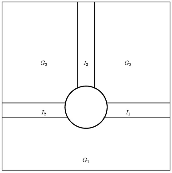
Figure 3. The blowing up and regularization approach separates ${\mathbb{R}}^2$ into seven regions $G_1$, $G_2$, $G_3$, $I_1$, $I_2,I_3$, and the circle.

Concerning the nonsmooth fold bifurcation that occurred in the Filippov system (16), after regularization, we have the following results.

Proposition 2. 

A saddle-node bifurcation occurs in the regularized system of (16). 

Proof. 

An equilibrium (ordinary equilibrium, boundary equilibrium, or pseudoequilibrium) of the Filippov system Z remains an equilibrium of its regularization $R_Z$ with the same type of stability [27]. For the three cases of the nonsmooth fold bifurcation, it is straightforward to derive the following results:

• When $x_0<x_1<x_3<x_2$ and $y_1<y_0<y_3<y_2$, the stable focus in region $G_3$ and the center equilibrium in region $G_1$ are preserved, while the pseudosaddle point on ${\mathsf{\Sigma }}_{+,y_0}$ becomes a saddle in region $I_1$ after regularization;
• When $x_0<x_1<x_3<x_2$ and $y_0=y_3$, the center equilibrium in region $G_1$ is preserved. After regularization, the boundary equilibrium of $F_3$, $\left(\frac{\delta +c_2}{\beta },y_0\right)$, is preserved but located at $\left(\frac{\delta +c_2}{\beta },y\right)$, where $y_0-\epsilon <y<y_0+\epsilon$;
• When $x_0<x_1<x_3<x_2$ and $y_0>y_3$, the regularized system $R_{\epsilon }$ only has a center equilibrium in region $G_1$.

In the entire process, as $y_0$ varies, the center stays unchanged, while the focus and the saddle collide and then disappear. Thus, a saddle-node bifurcation occurs. □

In the next section, we assign specific parameter values to the Filippov system (16) and its regularization, which helps us observe the difference in the dynamical behavior between the Filippov system (16) and its regularized system.

3.1.3. Simulation Results

The simulation results with the fixed parameter values $a=1,\beta =0.5,\eta =0.3$, $\delta =0.5,d=0.2,c_1=0.6,c_2=0.55,x_0=0.6$ are show in Figure 4. It is simple to observe that an admissible focus $(2.1,2.94)$ collides with the pseudosaddle $(10/7,2)$, and then both disappear, while the center equilibrium $(1,7/5)$ remains unchanged as $y_0$ varies. Therefore, a nonsmooth fold bifurcation occurs.

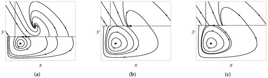
Figure 4. Nonsmooth fold bifurcation. Parameters are fixed at (a) $y_0=2$, (b) $y_0=2.94$, (c) $y_0=3$.

Under the chosen parameter values, the Filippov system (16) becomes

$$Z(x,y)=\left\{\begin{array}{cc}{F}_1(x,y),\hfill & (x,y)\in G_1,\hfill \\ F_2(x,y),\hfill & (x,y)\in G_2,\hfill \\ F_3(x,y),\hfill & (x,y)\in G_3,\hfill \end{array}\right.$$

(28a)

where

$$\begin{array}{cc}\hfill F_1(x,y)& =(x-0.5xy-0.3x,0.5xy-0.5y),\hfill \\ \hfill F_2(x,y)& =(x-0.5xy-0.3x+0.2x+0.6y,0.5xy-0.5y-0.6y),\hfill \\ \hfill F_3(x,y)& =(x-0.5xy-0.3x+0.55y,0.5xy-0.5y-0.55y).\hfill \end{array}$$

(28b)

Considering each part of the discontinuity set, we have the following results.

• Case I.
  Compared with the analysis in Section 3.1.2, the dynamics of the singular point ${\mathsf{\Sigma }}_{x_0,y_0}$ can be discussed in three different regions.
  For $0<\theta <\pi /2$,

  $${\theta }^{\prime }=cos\theta (0.5x_0{y}_0-0.5y_0-0.55y_0)-sin\theta (x_0-0.5x_0{y}_0-0.3x_0+0.55y_0);$$
  For $\pi /2<\theta <\pi$,

  $${\theta }^{\prime }=cos\theta (0.5x_0{y}_0-0.5y_0-0.6y_0)-sin\theta (x_0-0.5x_0{y}_0-0.3x_0+0.2x_0+0.6y_0);$$
  For $\pi <\theta <2\pi$,

  $${\theta }^{\prime }=cos\theta (0.5x_0{y}_0-0.5y_0)-sin\theta (x_0-0.5x_0{y}_0-0.3x_0).$$
• Case II.
  In region $I_1$, the slow manifold is given by

  $${\mathcal{M}}_1=\left\{(x,\psi )\in \mathbb{R}\times (0,\pi ):-sin\psi \left[{\displaystyle 0.5x{y}_0-0.5y_0-\frac{0.55y_0}{2}-\frac{0.55y_0}{2}\phi (cot\psi )}\right]=0\right\},$$

  which is a curve that connects $(x,\psi )=(2.1,0)$ and $(x,\psi )=(1,\pi )$. However, the point $(1,\pi )$ is not normally hyperbolic since

  $${\displaystyle \frac{\partial }{\partial \psi }\left[{\displaystyle -sin\psi (0.5xy-0.5y-\frac{0.55y}{2}-\frac{0.55y}{2}\phi (cot\psi ))}\right]{|}_{(1,\pi )}=0.}$$
  Therefore, it needs additional blow-up. First of all, this point is translated to the origin by $(x_1,{\psi }_1)=(x-1,\psi -\pi )$. Then, we perform the blowing up ${\psi }_1=ssin\vartheta$, $x_1=scos\vartheta$ with $s\ge 0$ and $\vartheta \in [\pi ,2\pi ]$. With the new coordinates, it gives the following:

  $$\begin{array}{ccc}\hfill & s^{\prime }=-sin(ssin\vartheta +\pi )sin\vartheta G(s,\vartheta ),\hfill & {\displaystyle {\vartheta }^{\prime }=-\frac{cos\vartheta sin(ssin\vartheta +\pi )}{s}G(s,\vartheta ),}\hfill \end{array}$$

  where ${\displaystyle G(s,\vartheta )=0.5(scos\vartheta +1)y-0.5y-\frac{0.55y}{2}-\frac{0.55y}{2}\phi (cot(ssin\vartheta +\pi ))}$. It is easy to check that $G(0,\vartheta )=0$ and ${\displaystyle \frac{\partial G}{\partial s}=0.5ycos\vartheta }$. Since ${\displaystyle \underset{s\to 0}{lim}\frac{{\vartheta }^{\prime }}{s}=0.5y{cos}^2\vartheta sin\vartheta }$, the angle component on the blowing up locus is decreasing for $\vartheta \in [\pi ,2\pi ]$.
• Case III.
  In region $I_2$, the slow manifold does not exist.
• Case IV.
  In region $I_3$, the slow manifold does not exist.

Now, we look at the global dynamics of the regularized system of (28) as the parameter $y_0$ varies. Recall that the plane ${\mathbb{R}}^2$ has been divided into seven regions after regularization. Next, we describe the dynamics of each region. First of all, for all the cases, the dynamics of the regularized system in $G_1,G_2,G_3$ are defined by the dynamics of $F_1,F_2,F_3$ in the respective region. In region $I_2$, there is no equilibrium, and the flow is smoothly connected to the flows of $G_1$ and $G_2$. The flow in region $I_3$ smoothly connects to the flows of $G_2$ and $G_3$. Subsequently, we consider the dynamics for the other regions for the three cases discussed in Proposition 3.

• For the case $y_1<y_0<y_3<y_2$, choosing $y_0=2$ since $y_3=2.94$ under the chosen parameter values, from the analysis of case I, we have the following on the circle:
  • When $0<\theta <\pi /2$, ${\theta }^{\prime }=-0.92sin\theta -1.5cos\theta <0$. Thus, $\theta$ is decreasing;
  • When $\pi /2<\theta <\pi$, ${\theta }^{\prime }=-1.14sin\theta -1.6cos\theta$. Then, ${\theta }^{\prime }<0$ for $\pi /2<\theta <{\theta }_0$, while ${\theta }^{\prime }>0$ for ${\theta }_0<\theta <\pi$. Here ${\theta }_0$ is given by ${\theta }^{\prime }{|}_{\theta ={\theta }_0}=0$;
  • When $\pi <\theta <2\pi$, ${\theta }^{\prime }=0.18sin\theta -0.4cos\theta$. Then, ${\theta }^{\prime }>0$ for $\pi <\theta <{\theta }_0$, while ${\theta }^{\prime }<0$ for ${\theta }_0<\theta <3\pi /2$, where ${\theta }_0$ is defined as the same as the previous case. When $3\pi /2<\theta <2\pi$, ${\theta }^{\prime }<0$.
  In region $I_1$, from the analysis of case II, it is easy to compute that the reduced problem has an equilibrium at $(x,\psi )=(10/7,{\psi }_0)$, and ${\displaystyle \phi (cot{\psi }_0)=-\frac{85}{385}}$. The flow goes in the positive direction of the x-axis if $\psi \in (0,{\psi }_0)$ and in the negative direction of the x-axis if $\psi \in ({\psi }_0,\pi )$; see Figure 5a.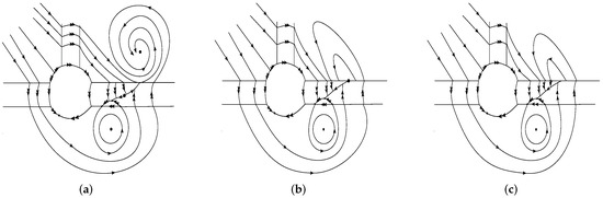
  

  Figure 5. Phase portrait of the regularization of system (28). The semicylinder represents the blowing up locus and the flows with a simple arrow and with a double arrow represent the slow and fast systems, respectively. Generated by (a) $y_0=2$, (b) $y_0=2.94$, (c) $y_0=3$.
• When $y_0=y_3=2.94$, on the circle, we have the following:
  • When $0<\theta <\pi /2$, ${\theta }^{\prime }=-1.155sin\theta -2.205cos\theta <0$;
  • When $\pi /2<\theta <\pi$, ${\theta }^{\prime }=-1.422sin\theta -2.352cos\theta$. Then, ${\theta }^{\prime }<0$ for $\pi /2<\theta <{\theta }_0$, while ${\theta }^{\prime }>0$ for ${\theta }_0<\theta <\pi$, where ${\theta }^{\prime }{|}_{\theta ={\theta }_0}=0$;
  • When $\pi <\theta <2\pi$, ${\theta }^{\prime }=0.462sin\theta -0.588cos\theta$. Therefore, ${\theta }^{\prime }>0$ for $\pi <\theta <{\theta }_0$, while ${\theta }^{\prime }<0$ for ${\theta }_0<\theta <3\pi /2$. For $3\pi /2<\theta <2\pi$, ${\theta }^{\prime }<0$.
  In region $I_1$, the reduced problem has one equilibrium at $(x,\psi )=(2.1,0)$. The vector points to the negative direction of the x-axis on the slow manifold.
• When $y_0>y_3$, for instance, $y_0=3$, then on the circle, we have the following:
  • When $0<\theta <\pi /2$, ${\theta }^{\prime }=-1.17sin\theta -2.25cos\theta <0$;
  • When $\pi /2<\theta <\pi$, ${\theta }^{\prime }=-1.44sin\theta -2.4cos\theta$. Then, ${\theta }^{\prime }<0$ for $\pi /2<\theta <{\theta }_0$, while ${\theta }^{\prime }>0$ for ${\theta }_0<\theta <\pi$;
  • When $\pi <\theta <2\pi$, ${\theta }^{\prime }=0.48sin\theta -0.6cos\theta$. For this case, when $\pi <\theta <3\pi /2$, $sin\theta <0,cos\theta <0$, there is a ${\theta }_0$ that ${\theta }^{\prime }=0$. Then, ${\theta }^{\prime }>0$ for $\pi <\theta <{\theta }_0$, while ${\theta }^{\prime }<0$ for ${\theta }_0<\theta <3\pi /2$. When $3\pi /2<\theta <2\pi$, $sin\theta <0,cos\theta >0$, we have ${\theta }^{\prime }<0$.
  In region $I_1$, the reduced problem has no equilibrium, and the vector of the slow manifold points to the negative direction of the x-axis; see Figure 5c.

3.2. The Filippov Avian-Only Model

Influenza is the most diversified in birds, particularly in wild waterfowl. Outbreaks of avian influenza in domestic poultry could, through a process of genetic reassortment, mutation, or both, introduce new influenza subtypes into the human population. In the context of widespread susceptibility, such an event could be the precursor of a pandemic. Since there is no cure for avian influenza, recommendations for precautions are both necessary and reasonable during poultry outbreaks. Many different types of mathematical models have been proposed for comparing interventions aimed at preventing and controlling an influenza pandemic [48,49,50]. Among all the preventative strategies, they have found that culling infected birds and those in contact with them is an effective method to control the spread [12,16,51]. Recently, an avian-only model has been constructed that incorporates culling only the infected birds, or both the infected and susceptible birds, depending on whether the numbers of infected and susceptible birds exceed the economic threshold values or not. The specific rules are as follows:

• When $y<y_0$, no control strategy is taken;
• When $y>y_0,x<x_0$, infected birds are culled at a rate of $c_2$;
• When $y>y_0,x>x_0$, infected birds are culled at a rate of $c_3$ and, meanwhile, susceptible birds are culled at a rate of $c_1$,

Therefore, an avian-only model can be described by the following Filippov system:

$$Z\left(X\right)=\left\{\begin{array}{cc}{F}_1\left(X\right),\hfill & \mathrm{if}X\in G_1,\hfill \\ F_2\left(X\right),\hfill & \mathrm{if}X\in G_2,\hfill \\ F_3\left(X\right),\hfill & \mathrm{if}X\in G_3,\hfill \end{array}\right.$$

(29a)

with

$$\begin{array}{cc}\hfill F_1(x,y)& =\left(rx\left({\displaystyle 1-\frac{x}{K}}\right)-\beta xy,\beta xy-\mu y-dy\right),\hfill \\ \hfill F_2(x,y)& =\left(rx\left({\displaystyle 1-\frac{x}{K}}\right)-\beta xy,\beta xy-\mu y-dy-c_{2}y\right),\hfill \\ \hfill F_3(x,y)& =\left(rx\left({\displaystyle 1-\frac{x}{K}}\right)-\beta xy-c_{1}x,\beta xy-\mu y-dy-c_{3}y\right),\hfill \end{array}$$

(29b)

in regions

$$G_1=\left\{(x,y)\right|y<y_0\},G_2=\left\{(x,y)\right|x<x_0,y>y_0\},G_3=\left\{(x,y)\right|x>x_0,y>y_0\}.$$

(29c)

The discontinuity set $\mathsf{\Sigma }={\mathsf{\Sigma }}_1\bigcup {\mathsf{\Sigma }}_2$ is defined the same as in Section 3.1, where

$${\mathsf{\Sigma }}_1=\{X\in {\mathbb{R}}^2:y-y_0=0\},{\mathsf{\Sigma }}_2=\{X\in {\mathbb{R}}^2:x-x_0=0,y-y_0\ge 0\}.$$

Here, x and y represent the numbers of susceptible and infected birds. $\beta >0$ denotes the transmission rate. $\mu >0$ is the natural death rate. $d>0$ is the disease-related death rate. Notice that the susceptible birds are assumed to be subject to logistic growth, where r is the intrinsic growth rate and K is the maximal carrying capacity. $x_0,y_0>0$ denote the respective susceptible threshold value and the infected threshold level. $r>c_1$, $c_2<c_3$ and $c_1,c_2,c_3>0$.

3.2.1. Equilibria and Bifurcation

System (29) in region $G_i$ has two types of equilibria: the disease-free equilibria $E_{i0}^1,E_{i0}^2$ and the endemic equilibrium $E_i,i=1,2,3$, which can be expressed as

$$\begin{array}{cc}\hfill E_{10}^1& =(0,0),E_{10}^2=(K,0),\hfill \\ \hfill E_1& =(x_1,y_1)=\left({\displaystyle \frac{\mu +d}{\beta },\frac{1}{\beta }\left({\displaystyle r-\frac{r(\mu +d)}{K\beta }}\right)}\right);\hfill \\ \hfill E_{20}^1& =(0,0),E_{20}^2=(K,0),\hfill \\ \hfill E_2& =(x_2,y_2)=\left({\displaystyle \frac{\mu +d+c_2}{\beta },\frac{1}{\beta }\left({\displaystyle r-\frac{r(\mu +d+c_2)}{K\beta }}\right)}\right);\hfill \\ \hfill E_{30}^1& =(0,0),E_{30}^2=(K,0),\hfill \\ \hfill E_3& =(x_3,y_3)=\left({\displaystyle \frac{\mu +d+c_3}{\beta },\frac{1}{\beta }\left({\displaystyle r-c_1-\frac{r(\mu +d+c_3)}{K\beta }}\right)}\right).\hfill \end{array}$$

In [16], they discuss the stability of all the equilibria of 16 different cases depending on the values of $x_i$ and $y_i$, $i=0,1,2,3$. In this work, we only concentrate on the bifurcation analysis of the case

$$\begin{array}{c}\hfill x_1<x_2<x_3<x_0\mathrm{with}{y}_0<y_3<y_2<y_1,\mathrm{or}{y}_3<y_0<y_2<y_1,\\ \hfill \mathrm{or}{y}_3<y_2<y_0<y_1,\mathrm{or}{y}_3<y_2<y_1<y_0.\end{array}$$

(30)

The other cases are similar, so we omit their analysis here. Moreover, in this paper, we only discuss the case when the unique endemic equilibrium $E_i$ exists. Then, the disease-free equilibrium $E_{i0}^1$ is always unstable, while the equilibrium $E_i$ in region $G_i$ is globally asymptotically stable, $i=1,2,3$.

Besides, for our analysis, the condition

$$\frac{r}{\beta }\left({\displaystyle 1-\frac{x_0}{K}}\right)<y_0$$

(31)

is imposed.

Proposition 3. 

A persistence bifurcation occurs in system (29) under the condition $x_1<x_2<x_3<x_0$. Specifically, the following holds:

• When $x_1<x_2<x_3<x_0$ and $y_0<y_2$, system (29) has a stable focus;
• When $x_1<x_2<x_3<x_0$ and $y_0=y_2$, this focus turns into a boundary equilibrium;
• When $x_1<x_2<x_3<x_0$ and $y_3<y_2<y_0<y_1$, the boundary equilibrium turns into a pseudonode.

The proof of the existence and stability of each equilibrium is derived from the work in [16,52], and the proof of this proposition can directly be derived from it.

Next, we study the regularization of the avian-only system (29).

3.2.2. Regularization

Again, the discontinuity set $\mathsf{\Sigma }$ of system (29) can be divided into the simple discontinuity ${\mathsf{\Sigma }}_{+,y_0}\cup {\mathsf{\Sigma }}_{-,y_0}\cup {\mathsf{\Sigma }}_{x_0,+}$ and the nonsimple discontinuity ${\mathsf{\Sigma }}_{x_0,y_0}$. Subsequently, the regularization method is applied separately to each part of the discontinuity set of the Filippov avian-only model (29).

• Case I.
  For the nonsimple discontinuity ${\mathsf{\Sigma }}_{x_0,y_0}$, it is firstly transformed into a simple discontinuity by the map (19). Then, the dynamics are given by

  $${\theta }^{\prime }=-f_{i}sin\theta +g_{i}cos\theta ,F_i=(f_i,g_i),i=1,2,3.$$
  For $0<\theta <\pi /2$, $F_3(x,y)=\left(rx\left({\displaystyle 1-\frac{x}{K}}\right)-\beta xy-c_{1}x,\beta xy-\mu y-dy-c_{3}y\right)$, the dynamics are given by

  $${\theta }^{\prime }=cos\theta (\beta x_0{y}_0-\mu y_0-d{y}_0-c_3{y}_0)-sin\theta \left(r{x}_0\left({\displaystyle 1-\frac{x_0}{K}}\right)-\beta x_0{y}_0-c_1{x}_0\right);$$
  For $\pi /2<\theta <\pi$, $F_2(x,y)=\left(rx\left({\displaystyle 1-\frac{x}{K}}\right)-\beta xy,\beta xy-\mu y-dy-c_{2}y\right)$, the dynamics is

  $${\theta }^{\prime }=cos\theta (\beta x_0{y}_0-\mu y_0-d{y}_0-c_2{y}_0)-sin\theta \left(r{x}_0\left({\displaystyle 1-\frac{x_0}{K}}\right)-\beta x_0{y}_0\right);$$
  For $\pi <\theta <2\pi$, $F_1(x,y)=\left(rx\left({\displaystyle 1-\frac{x}{K}}\right)-\beta xy,\beta xy-\mu y-dy\right)$, the dynamics are

  $${\theta }^{\prime }=cos\theta (\beta x_0{y}_0-\mu y_0-d{y}_0)-sin\theta \left(r{x}_0\left({\displaystyle 1-\frac{x_0}{K}}\right)-\beta x_0{y}_0\right).$$
  Now, we apply the regularization method to the other boundaries.
• Case II.
  For the Filippov system

  $$\begin{array}{c}\hfill Z_1(x,y)=\left\{\begin{array}{cc}\hfill F_1(x,y),& (x,y)\in G_1,\hfill \\ \hfill F_3(x,y),& (x,y)\in G_3,\hfill \end{array}\right.\end{array}$$

  with the boundary ${\mathsf{\Sigma }}_{+,y_0}=\left\{(x,y_0)\right|y=y_0,x>x_0\}$, the regularized vector field is

  $$R_{Z_1}=\left[{\displaystyle \frac{1}{2}+\frac{1}{2}\phi \left({\displaystyle \frac{y-y_0}{\epsilon }}\right)}\right]F_3(x,y)+\left[{\displaystyle \frac{1}{2}-\frac{1}{2}\phi \left({\displaystyle \frac{y-y_0}{\epsilon }}\right)}\right]F_1(x,y).$$

  (32)
  Around region ${\mathsf{\Sigma }}_{+,y_0}$, the differential system is given by

  $$\begin{array}{cc}\hfill \dot{x}=& \left[{\displaystyle \frac{1}{2}+\frac{1}{2}\phi \left({\displaystyle \frac{y-y_0}{\epsilon }}\right)}\right]\left(rx\left({\displaystyle 1-\frac{x}{K}}\right)-\beta xy-c_{1}x\right)-\left[{\displaystyle \frac{1}{2}-\frac{1}{2}\phi \left({\displaystyle \frac{y-y_0}{\epsilon }}\right)}\right]\beta xy\hfill \\ \hfill & +\left[{\displaystyle \frac{1}{2}-\frac{1}{2}\phi \left({\displaystyle \frac{y-y_0}{\epsilon }}\right)}\right]rx\left({\displaystyle 1-\frac{x}{K}}\right)\hfill \\ \hfill =& {\displaystyle rx\left({\displaystyle 1-\frac{x}{K}}\right)-\beta xy-\frac{c_{1}x}{2}-\frac{c_{1}x}{2}\phi \left({\displaystyle \frac{y-y_0}{\epsilon }}\right),}\hfill \\ \hfill \dot{y}=& \left[{\displaystyle \frac{1}{2}+\frac{1}{2}\phi \left({\displaystyle \frac{y-y_0}{\epsilon }}\right)}\right](\beta xy-\mu y-dy-c_{3}y)+\left[{\displaystyle \frac{1}{2}-\frac{1}{2}\phi \left({\displaystyle \frac{y-y_0}{\epsilon }}\right)}\right](\beta xy-\mu y)\hfill \\ \hfill & -\left[{\displaystyle \frac{1}{2}-\frac{1}{2}\phi \left({\displaystyle \frac{y-y_0}{\epsilon }}\right)}\right]dy\hfill \\ \hfill =& {\displaystyle \beta xy-\mu y-dy-\frac{c_{3}y}{2}-\frac{c_{3}y}{2}\phi \left({\displaystyle \frac{y-y_0}{\epsilon }}\right).}\hfill \end{array}$$

  (33)
  Then, system (33) can be transformed into a singular perturbation problem by

  $$y=y_0+\eta cos\psi ,\epsilon =\eta sin\psi ,$$

  (34)

  where $\eta \ge 0$ and $\psi \in [0,\pi ]$, which is

  $$\begin{array}{cc}\hfill \eta \dot{\psi }=& -sin\psi \left[{\displaystyle \beta x(y_0+\eta cos\psi )-\mu (y_0+\eta cos\psi )-d(y_0+\eta cos\psi )-\frac{c_3{y}_0}{2}}\right.\hfill \\ \hfill & \left.{\displaystyle -\frac{c_3\eta cos\psi }{2}-\frac{c_3(y_0+\eta cos\psi )}{2}\phi (cot\psi )}\right],\hfill \\ \hfill \dot{x}=& {\displaystyle rx\left({\displaystyle 1-\frac{x}{K}}\right)-\beta x(y_0+\eta cos\psi )-\frac{c_{1}x}{2}+\frac{c_{1}x}{2}\phi (cot\psi ).}\hfill \end{array}$$
  Now, $\epsilon =0$ is represented by $\eta =0$. The slow manifold is given by ${\mathcal{M}}_1=\left\{(x,\psi )\in \mathbb{R}\times (0,\pi ):-sin\psi \left[{\displaystyle \beta x{y}_0-\mu y_0-d{y}_0-\frac{c_3}{2}{y}_0-\frac{\phi (cot\psi )}{2}{c}_3{y}_0}\right]=0\right\}$, i.e., ${\displaystyle \phi (cot\psi )=\frac{2\beta x{y}_0-2\mu y_0-2d{y}_0-c_3{y}_0}{c_3{y}_0}=\frac{2\beta x-2\mu -2d-c_3}{c_3}}$. Since ${\displaystyle x>x_0>x_3=\frac{\mu +d+c_3}{\beta }}$, $\phi (cot\psi )>1$, there is no slow manifold.
• Case III.
  For the Filippov system

  $$\begin{array}{c}\hfill Z_2(x,y)=\left\{\begin{array}{cc}\hfill F_1(x,y),& (x,y)\in G_1,\hfill \\ \hfill F_2(x,y),& (x,y)\in G_2,\hfill \end{array}\right.\end{array}$$

  with the boundary ${\mathsf{\Sigma }}_{-,y_0}=\left\{(x,y_0)\right|y=y_0,x<x_0\}$, the regularized system is

  $$R_{Z_2}=\left[{\displaystyle \frac{1}{2}+\frac{1}{2}\phi \left({\displaystyle \frac{y-y_0}{\epsilon }}\right)}\right]F_2(x,y)+\left[{\displaystyle \frac{1}{2}-\frac{1}{2}\phi \left({\displaystyle \frac{y-y_0}{\epsilon }}\right)}\right]F_1(x,y).$$

  (35)
  Around region ${\mathsf{\Sigma }}_{-,y_0}$, the differential system is given by

  $$\begin{array}{cc}\hfill \dot{x}& =rx\left({\displaystyle 1-\frac{x}{K}}\right)-\beta xy,\hfill \\ \hfill \dot{y}& {\displaystyle =\beta xy-\mu y-dy-\frac{c_{2}y}{2}-\frac{c_{2}y}{2}\phi \left(\frac{y-y_0}{\epsilon }\right).}\hfill \end{array}$$

  (36)
  Applying the transformation (34), we obtain

  $$\begin{array}{cc}\hfill \eta \dot{\psi }=& -sin\psi \left[{\displaystyle \beta x(y_0+\eta cos\psi )-\mu (y_0+\eta cos\psi )-d(y_0+\eta cos\psi )-\frac{c_2{y}_0}{2}}\right.\hfill \\ \hfill & \left.{\displaystyle +\frac{c_2\eta cos\psi }{2}-\frac{c_2(y_0+\eta cos\psi )}{2}\phi (cot\psi )}\right],\hfill \\ \hfill \dot{x}=& rx\left({\displaystyle 1-\frac{x}{K}}\right)-\beta x(y_0+\eta cos\psi ).\hfill \end{array}$$
  For $\epsilon =0$, the slow manifold is ${\mathcal{M}}_2=\left\{(x,\psi )\in \mathbb{R}\times (0,\pi ):-sin\psi \left[{\displaystyle \beta x{y}_0-\mu y_0-d{y}_0-\frac{c_2{y}_0}{2}-\phi (cot\psi )\frac{c_2{y}_0}{2}}\right]=0\right\}$, i.e., ${\displaystyle \alpha (cot\psi )=\frac{2\beta x-2\mu -2d-c_2}{c_2}}$. The slow manifold is a curve that connects $(x,\psi )=\left({\displaystyle \frac{\mu +d+c_2}{\beta },0}\right)$ and $(x,\psi )=\left({\displaystyle \frac{\mu +d}{\beta },\pi }\right)$.
• Case IV.
  For the Filippov system

  $$\begin{array}{c}\hfill Z_3(x,y)=\left\{\begin{array}{cc}\hfill F_2(x,y),& (x,y)\in G_2,\hfill \\ \hfill F_3(x,y),& (x,y)\in G_3,\hfill \end{array}\right.\end{array}$$

  with the boundary ${\mathsf{\Sigma }}_{x_0,+}=\left\{(x_0,y)\right|x=x_0,y>y_0\}$, its regularized system is

  $$R_{Z_3}=\left[{\displaystyle \frac{1}{2}+\frac{1}{2}\phi \left({\displaystyle \frac{x-x_0}{\epsilon }}\right)}\right]F_3(x,y)+\left[{\displaystyle \frac{1}{2}-\frac{1}{2}\phi \left({\displaystyle \frac{x-x_0}{\epsilon }}\right)}\right]F_2(x,y).$$

  (37)
  Around region ${\mathsf{\Sigma }}_{x_0,+}$, the differential system is given by

  $$\begin{array}{cc}\hfill \dot{x}& {\displaystyle =rx\left({\displaystyle 1-\frac{x}{K}}\right)-\beta xy-\frac{c_{1}x}{2}-\frac{c_{1}x}{2}\phi \left({\displaystyle \frac{x-x_0}{\epsilon }}\right),}\hfill \\ \hfill \dot{y}& {\displaystyle =\beta xy-\mu y-dy-\frac{c_{2}y+c_{3}y}{2}+\frac{c_{2}y-c_{3}y}{2}\phi \left({\displaystyle \frac{x-x_0}{\epsilon }}\right).}\hfill \end{array}$$

  (38)
  Then, system (38) is transformed into a singular perturbation problem by map (27) as

  $$\begin{array}{cc}\hfill \eta \dot{\psi }=& -sin\psi \left[{\displaystyle r(x_0+\eta cos\psi )\left({\displaystyle 1-\frac{x_0+\eta cos\psi }{K}}\right)-\beta (x_0+\eta cos\psi )y-\frac{c_1{x}_0}{2}}\right.\hfill \\ \hfill & \left.{\displaystyle -\frac{c_1\eta cos\psi }{2}-\frac{c_1(x_0+\eta cos\psi )}{2}\phi (cot\psi )}\right],\hfill \\ \hfill \dot{y}=& {\displaystyle \beta (x_0+\eta cos\psi )y-\mu y-dy-\frac{c_{2}y+c_{3}y}{2}+\frac{c_{2}y-c_{3}y}{2}\phi (cot\psi ).}\hfill \end{array}$$
  For $\epsilon =0$, the slow manifold is given by ${\mathcal{M}}_3=\left\{(\psi ,y)\in (0,\pi )\times \mathbb{R}:-sin\psi \left({\displaystyle r{x}_0\left({\displaystyle 1-\frac{x_0}{K}}\right)-\beta x_{0}y-\frac{c_1{x}_0}{2}-\frac{c_1{x}_0}{2}\phi (cot\psi }\right)=0\right\}$, i.e., ${\displaystyle \phi (cot\psi )=\frac{2\left(r{x}_0\left({\displaystyle 1-\frac{x_0}{K}}\right)-\beta x_{0}y\right)-c_1{x}_0}{c_1{x}_0}=\frac{2\left(r\left({\displaystyle 1-\frac{x_0}{K}}\right)-\beta y\right)-c_1}{c_1}}$. Taking account of the condition (31) and $y>y_0$, it gives $\phi (cot\psi )<-1$. There is no slow manifold.

Considering persistence bifurcation happened in the Filippov system (29), after regularization, we have the following conclusion.

Proposition 4. 

Persistence bifurcation disappears after regularization. 

Proof. 

Since the quantity and stability of the equilibria of Z do not change after regularization, it is straightforward to derive the following results:

• When $x_1<x_2<x_3<x_0$ and $y_0<y_2$, the stable focus in region $G_2$ preserves after regularization;
• When $x_1<x_2<x_3<x_0$ and $y_0=y_2$, after regularization, the boundary equilibrium of $F_2$$\left(\frac{\mu +d+c_2}{\beta },y_0\right)$ is preserved but located at $\left(\frac{\mu +d+c_2}{\beta },y\right)$, where $y_0-\epsilon <y<y_0+\epsilon$;
• When $x_1<x_2<x_3<x_0$ and $y_3<y_2<y_0<y_1$, the regularized system $R_Z$ has a stable node in region $I_2$.

In the entire process, as $y_0$ varies, the regularized system $R_Z$ always has a stable equilibrium but is located at different regions. Besides, it is simple to check that system $R_Z$ has no other equilibria. Since no qualitative property changes as the parameter $y_0$ varies, there is no bifurcation occurring in system $R_Z$. □

In the next section, we fix specific parameter values to observe the persistence bifurcation and its qualitative properties after regularization.

3.2.3. Simulation Results

The simulation results are given in Figure 6 when the parameter values are fixed as $r=0.0047,\beta =2\times {10}^{-5},K=600,\mu =1.2\times {10}^{-3},d=4\times {10}^{-3},c_1=0.001$, $c_2=0.003$, $c_3=0.006,x_0=570$. It is simple to observe from Figure 6 that an admissible focus $(410,74.416)$ turns into a pseudonode $(344.68,100)$ as $y_0$ varies, while no extra equilibria appear. Therefore, a persistence bifurcation occurs in system (29).

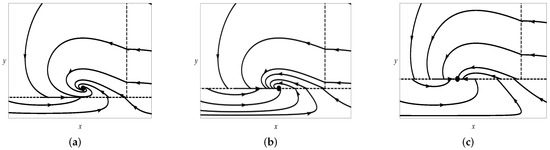
Figure 6. Persistence bifurcation. Generated by (a) $y_0=50$, (b) $y_0=y_2$, (c) $y_0=100$.

Now, we look at what happens to this bifurcation after regularization. Under the chosen parameter values, the Filippov system (29) becomes

$$Z(x,y)=\left\{\begin{array}{cc}{F}_1(x,y),\hfill & (x,y)\in G_1,\hfill \\ F_2(x,y),\hfill & (x,y)\in G_2,\hfill \\ F_3(x,y),\hfill & (x,y)\in G_3,\hfill \end{array}\right.$$

(39a)

where

$$\begin{array}{cc}\hfill F_1(x,y)=& \left(0.0047x\left({\displaystyle 1-\frac{x}{600}}\right)-2\times {10}^{-5}xy,2\times {10}^{-5}xy-1.2\times {10}^{-3}y\right.\hfill \\ \hfill & \left.-4\times {10}^{-3}y\right),\hfill \\ \hfill F_2(x,y)=& \left(0.0047x\left({\displaystyle 1-\frac{x}{600}}\right)-2\times {10}^{-5}xy,2\times {10}^{-5}xy-1.2\times {10}^{-3}y\right.\hfill \\ \hfill & \left.-4\times {10}^{-3}y-0.003y\right),\hfill \\ \hfill F_3(x,y)=& \left(0.0047x\left({\displaystyle 1-\frac{x}{600}}\right)-2\times {10}^{-5}xy-0.001x,2\times {10}^{-5}xy-1.2\times {10}^{-3}y\right.\hfill \\ \hfill & \left.-4\times {10}^{-3}y-0.006y\right).\hfill \end{array}$$

(39b)

Considering each part of the discontinuity set, we have the following results.

• Case I.
  Compared with the analysis in Section 3.1.2, the dynamics of ${\mathsf{\Sigma }}_{x_0,y_0}$ can be discussed in three different regions.
  For $0<\theta <\pi /2$,

  $$\begin{array}{cc}\hfill {\theta }^{\prime }=& cos\theta (2\times {10}^{-5}{x}_0{y}_0-1.2\times {10}^{-3}{y}_0-4\times {10}^{-3}{y}_0-0.006y_0)-sin\theta \hfill \\ \hfill & \left(0.0047x_0\left({\displaystyle 1-\frac{x_0}{600}}\right)-2\times {10}^{-5}{x}_0{y}_0-0.001x_0\right);\hfill \end{array}$$
  For $\pi /2<\theta <\pi$,

  $$\begin{array}{cc}\hfill {\theta }^{\prime }=& cos\theta (2\times {10}^{-5}{x}_0{y}_0-1.2\times {10}^{-3}{y}_0-4\times {10}^{-3}{y}_0-0.003y_0)-sin\theta \hfill \\ \hfill & \left(0.0047x_0\left({\displaystyle 1-\frac{x_0}{600}}\right)-2\times {10}^{-5}{x}_0{y}_0\right);\hfill \end{array}$$
  For $\pi <\theta <2\pi$,

  $$\begin{array}{cc}\hfill {\theta }^{\prime }=& cos\theta (2\times {10}^{-5}{x}_0{y}_0-1.2\times {10}^{-3}{y}_0-4\times {10}^{-3}{y}_0)-sin\theta \left(0.0047x_0\right.\hfill \\ \hfill & \left.\left({\displaystyle 1-\frac{x_0}{600}}\right)-2\times {10}^{-5}{x}_0{y}_0\right).\hfill \end{array}$$
• Case II.
  In region $I_1$, the slow manifold is an empty set for this case.
• Case III.
  In region $I_2$, the slow manifold is ${\mathcal{M}}_2=\{(x,\psi )\in \mathbb{R}\times (0,\pi ):u(x,\psi )=0\}$, where $u(x,\psi )=-sin\psi \left[{\displaystyle 2\times {10}^{-5}x{y}_0-1.2\times {10}^{-3}{y}_0-4\times {10}^{-3}{y}_0-\frac{0.003y_0}{2}-}\right.\left.{\displaystyle \frac{0.003y_0}{2}\phi (cot\psi )}\right]$. It is a curve connecting the points $(x,\psi )=(260,\pi )$ and $(x,\psi )=(410,0)$.
  Notice that the point $(260,\pi )$ is not normally hyperbolic since

  $${\displaystyle \frac{\partial u(x,\psi )}{\partial \psi }{|}_{(260,\pi )}=0.}$$
  Therefore, it needs additional blow-up. First of all, we translate this point to the origin with $(x_2,{\psi }_2)=(x-260,\psi -\pi )$. Next, the blowing up ${\psi }_2=ssin\vartheta$, $x_2=scos\vartheta$ with $s\ge 0$ and $\vartheta \in [\pi ,2\pi ]$ is performed to this point. With new coordinates, it gives

  $$\begin{array}{ccc}\hfill & s^{\prime }=-sin(ssin\vartheta +\pi )sin\vartheta G(s,\vartheta ),\hfill & {\displaystyle {\vartheta }^{\prime }=-\frac{cos\vartheta sin(ssin\vartheta +\pi )}{s}G(s,\vartheta ),}\hfill \end{array}$$

  where ${\displaystyle G(s,\vartheta )=2\times {10}^{-5}(scos\vartheta +260)y_0-1.2\times {10}^{-3}{y}_0-4\times {10}^{-3}{y}_0-\frac{0.003y_0}{2}-\frac{0.003y_0}{2}\phi (cot(ssin\vartheta +\pi ))}$. One verifies that $G(0,\vartheta )=0$ and ${\displaystyle \frac{\partial G}{\partial s}=2\times {10}^{-5}{y}_{0}cos\vartheta }$. Thus, ${\displaystyle \underset{s\to 0}{lim}\frac{{\vartheta }^{\prime }}{s}=2\times {10}^{-5}{y}_0{cos}^2\vartheta sin\vartheta }$. This means that the angle component is decreasing for $\vartheta \in [\pi ,2\pi ]$.
• Case IV.
  In region $I_3$, the slow manifold is an empty set.

Now, we look at the global dynamics of the regularized system of (39) as the parameter $y_0$ varies. The dynamics of $R_Z$ in $G_1,G_2,G_3$ are defined by the dynamics of $F_1,F_2,F_3$ in the respective region. In region $I_1$, there is no equilibrium, and the flow is continuously connected to the flows of $G_1$ and $G_3$. The flow in region $I_3$ continuously connects to the flows of $G_2$ and $G_3$. Subsequently, we look at the dynamics in the other regions for the three cases discussed in Proposition 4.

• For the case $y_0<y_2$, considering $y_0=50$ since $y_2=74.416$ under the chosen parameter values, from the analysis of case I, on the circle, the following holds:
  • When $0<\theta <\pi /2$, ${\theta }^{\prime }=1.00605sin\theta +0.01cos\theta >0$;
  • When $\pi /2<\theta <\pi$, ${\theta }^{\prime }=1.00605sin\theta +0.16cos\theta$. For this case, there exists a ${\theta }_0$ such that ${\theta }^{\prime }=0$. Therefore, ${\theta }^{\prime }>0$ for $\pi /2<\theta <{\theta }_0$, while ${\theta }^{\prime }<0$ for ${\theta }_0<\theta <\pi$;
  • When $\pi <\theta <2\pi$, ${\theta }^{\prime }=1.00606sin\theta +0.31cos\theta$. Thus, ${\theta }^{\prime }<0$ for $\pi <\theta <3\pi /2$ and $3\pi /2<\theta <{\theta }_0$, while ${\theta }^{\prime }>0$ for ${\theta }_0<\theta <2\pi$, where ${\theta }_0$ has the same definition as the previous case.
  In region $I_2$, the reduced flow goes in the positive direction of the x-axis; see Figure 7a.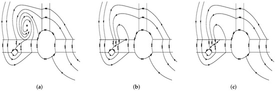
  

  Figure 7. Phase portraits of the regularized system $R_Z$. Generated by (a) $y_0=50$, (b) $y_0=y_2=74.416$, (c) $y_0=100$.
• When $y_0=y_2=74.416$, on the circle, the following holds:
  • When $0<\theta <\pi /2$, ${\theta }^{\prime }=1.28sin\theta +0.015cos\theta >0$;
  • When $\pi /2<\theta <\pi$, ${\theta }^{\prime }=0.71sin\theta +0.23cos\theta$. Then ${\theta }^{\prime }>0$ for $\pi /2<\theta <{\theta }_0$, while ${\theta }^{\prime }<0$ for ${\theta }_0<\theta <\pi$, where ${\theta }^{\prime }{|}_{\theta ={\theta }_0}=0$;
  • When $\pi <\theta <2\pi$, ${\theta }^{\prime }=0.71sin\theta +0.46cos\theta$. Thus, ${\theta }^{\prime }<0$ for $\pi <\theta <3\pi /2$ and $3\pi /2<\theta <{\theta }_0$, while ${\theta }^{\prime }>0$ for ${\theta }_0<\theta <2\pi$.
  In region $I_2$, the reduced problem has an equilibrium at $(x,\psi )=(410,0)$. The flow goes in the positive direction of the x-axis; see Figure 7b.
• When $y_3<y_2<y_0<y_1$, for instance, $y_0=100$, then on the circle, the following holds:
  • When $0<\theta <\pi /2$, ${\theta }^{\prime }=1.57sin\theta +0.02cos\theta >0$;
  • When $\pi /2<\theta <\pi$, ${\theta }^{\prime }=1.006sin\theta +0.32cos\theta$. Then, ${\theta }^{\prime }>0$ for $\pi /2<\theta <{\theta }_0$, while ${\theta }^{\prime }<0$ for ${\theta }_0<\theta <\pi$;
  • When $\pi <\theta <2\pi$, ${\theta }^{\prime }=1.006sin\theta +0.62cos\theta$. Thus, ${\theta }^{\prime }<0$ for $\pi <\theta <3\pi /2$ and $3\pi /2<\theta <{\theta }_0$, while ${\theta }^{\prime }>0$ for ${\theta }_0<\theta <2\pi$.
  In region $I_2$, the reduced problem has an equilibrium at $(x,\psi )=(344.68,$ ${\psi }_0)$, and ${\displaystyle \phi (cot{\psi }_0)=\frac{242}{1875}}$, and the flow goes in the positive direction of the x-axis if $\psi \in ({\psi }_0,\pi )$ and goes in the negative direction of the x-axis if $\psi \in (0,{\psi }_0)$; see Figure 7c.

4. Conclusions and Future Work

In this paper, we apply the regularization approach to the Filippov system with rich discontinuity boundaries. This type of system appears in applications of various natures: control theory, classical electromagnetism theory, and relay feedback systems. Two specific examples of such types of systems are investigated in this work. We discuss the bifurcations of these systems and the corresponding ones after regularization. The nonsmooth fold bifurcation that occurs in the plant disease model becomes a saddle-node bifurcation. The persistence bifurcation happening in the Filippov avian-only model disappears after regularization. During the regularization process, the singular perturbation theory and the blow-up technique play an important role.

A further extension of this work is to investigate the more complicated bifurcations of such types of Filippov systems by regularization approach, such as the bifurcations involving limit cycles.

References

- Bernardo, M.D.; Budd, C.J.; Champneys, A.R.; Kowalczyk, P. Piecewise-Smooth Dynamical Systems: Theory and Applications, 1st ed.; Springer: Berlin/Heidelberg, Germany, 2008. [Google Scholar]
- Bernardo, M.D.; Pagano, D.J.; Ponce, E. Non-hyperbolic Boundary Equilibrium Bifurcations in Planar Filippov Systems: A Case Study Approach. Int. J. Bifurc. Chaos 2008, 18, 1377–1392. [Google Scholar] [CrossRef]
- Biák, M.; Hanus, T.; Janovská, D. Some applications of Filippov’s dynamical systems. J. Comput. Appl. Math. 2013, 254, 132–143. [Google Scholar] [CrossRef]
- Goh, B.S. Stability in Models of Mutualism. Am. Nat. 1979, 113, 261–275. [Google Scholar] [CrossRef]
- Liu, L.R.; Xiang, C.C.; Tang, G.Y. Dynamics Analysis of Periodically Forced Filippov Holling II Prey-Predator Model With Integrated Pest Control. IEEE Access 2019, 7, 113889–113900. [Google Scholar] [CrossRef]
- Qin, W.J.; Tan, X.W.; Shi, X.T.; Chen, J.H.; Liu, X.Z. Dynamics and Bifurcation Analysis of a Filippov Predator-Prey Ecosystem in a Seasonally Fluctuating Environment. Int. J. Bifurc. Chaos 2019, 29, 1–16. [Google Scholar] [CrossRef]
- Filippov, A.F. Differential Equations with Discontinuous Righthand Sides, 1st ed.; Springer: Dordrecht, The Netherlands, 1988. [Google Scholar]
- Agrawal, J.; Moudgalya, K.M.; Pani, A.K. Sliding motion of discontinuous dynamical systems described by semi-implicit index one differential algebraic equations. Chem. Eng. Sci. 2006, 61, 4722–4731. [Google Scholar] [CrossRef]
- Chen, F.D. Permanence of periodic Holling type Predator-Prey system with stage structure for prey. Appl. Math. Comput. 2006, 182, 1849–1860. [Google Scholar] [CrossRef]
- Chen, L.J.; Chen, F.D.; Chen, L.J. Qualitative analysis of a predator-prey model with Holling type II functional response incorporating a constant prey refuge. Nonlinear Anal. Real World Appl. 2010, 11, 246–252. [Google Scholar] [CrossRef]
- Buzzi, C.A.; Silva, P.R.; Teixeira, M.A. Slow-fast systems on algebraic varieties bordering piecewise-smooth dynamical systems. Bull. Sci. 2012, 136, 444–462. [Google Scholar] [CrossRef][Green Version]
- Chong, N.; Smith, R. Modeling avian influenza using Filippov systems to determine culling of infected birds and quarantine. Nonlinear Anal. Real World Appl. 2015, 24, 196–218. [Google Scholar] [CrossRef]
- Huang, L.H.; Ma, H.L.; Wang, J.F.; Huang, C.X. Global dynamics of a Filippov plant disease model with an economic threshold of infected-susceptible ratio. J. Appl. Anal. Comput. 2020, 10, 2263–2277. [Google Scholar] [CrossRef]
- Teixeira, M.A.; Silva, P.R. Regularization and singular perturbation techniques for non-smooth systems. Phys. Nonlinear Phenom. 2012, 241, 1948–1955. [Google Scholar] [CrossRef]
- Chen, C.; Chen, X. Rich Sliding Motion and Dynamics in a Filippov Plant-Disease System. Int. J. Bifurc. Chaos 2018, 28, 1850012. [Google Scholar] [CrossRef]
- Yang, Y.P.; Wang, L.J. Global Dynamics and Rich Sliding Motion in an Avian-Only Filippov System in Combating Avian Influenza. Int. Bifurc. Chaos 2020, 30, 2050008. [Google Scholar] [CrossRef]
- Cao, N.B.; Zhang, Y.; Liu, X. Dynamics and Bifurcations in Filippov Type of Competitive and Symbiosis Systems. Int. J. Bifurc. Chaos 2022, 32, 1–21. [Google Scholar] [CrossRef]
- Dercole, F.; Rossa, F.D.; Colombo, A.; Kuznetsov, Y.A. Two Degenerate Boundary Equilibrium Bifurcations in Planar Filippov Systems. SIAM J. Appl. Dyn. Syst. 2011, 10, 1525–1553. [Google Scholar] [CrossRef][Green Version]
- Efstathiou, K.; Liu, X.; Broer, H.W. The Boundary-Hopf-Fold Bifurcation in Filippov Systems. SIAM J. Appl. Dyn. Syst. 2015, 14, 914–941. [Google Scholar] [CrossRef][Green Version]
- Kuznetsov, Y.A.; Rinaldi, S.; Gragnani, A. One-Parameter Bifurcations in Planar Filippov Systems. Int. J. Bifurc. Chaos 2003, 13, 1–50. [Google Scholar] [CrossRef]
- Jelbart, S.; Kristiansen, K.U.; Wechselberger, M. Singularly Perturbed Boundary-Equilibrium Bifurcations. Nonlinearity 2021, 34, 7371–7414. [Google Scholar] [CrossRef]
- Jelbart, S.; Kristiansen, K.U.; Wechselberger, M. Singularly Perturbed Boundary-Focus Bifurcations. J. Differ. Equ. 2021, 296, 412–492. [Google Scholar] [CrossRef]
- Kaklamanos, P.; Kristiansen, K.U. Regularization and Geometry of Piece-wise Smooth Systems with Intersecting Discontinuity Sets. SIAM J. Appl. Dyn. Syst. 2019, 18, 1225–1264. [Google Scholar] [CrossRef]
- Leine, R.I.; Nijmeijer, H. Dynamics and Bifurcations of Non-Smooth Mechanical Systems, 1st ed.; Springer: Berlin/Heidelberg, Germany, 2004. [Google Scholar]
- Lin, Q.F. Dynamic behaviors of a commensal symbiosis model with non-monotonic functional response and non-selective harvesting in a partial closure. Commun. Math. Biol. Neurosci. 2018, 2018, 1–15. [Google Scholar]
- Liu, X. The Discontinuous Hopf-Transversal System and Its Geometric Regularization. Ph.D. Thesis, University of Groningen, Groningen, The Netherlands, 2013. [Google Scholar]
- Sotomayor, J.; Teixeira, M.A. Regularization of Discontinuous Vector Fields. In Proceedings of the International Conference on Differential Equations, Lisboa, Portugal, 18–23 August 1996. [Google Scholar]
- Buzzi, C.A.; Silva, P.R.; Teixeira, M.A. A singular approach to discontinuous vector fields on the plane. J. Differ. Equ. 2006, 231, 633–655. [Google Scholar] [CrossRef]
- Guardia, M.; Seara, T.M.; Teixeira, M.A. Generic bifurcations of low codimension of planar Filippov systems. J. Differ. Equ. 2011, 250, 1967–2023. [Google Scholar] [CrossRef]
- Jacquemard, A.; Teixeira, M.A. On singularities of discontinuous vector fields. Bull. Des. Sci. Math. 2003, 127, 611–633. [Google Scholar] [CrossRef]
- Llibre, J.; Silva, P.R.; Teixeira, M.A. Regularization of Discontinuous Vector Fields on R3 via Singular Perturbation. J. Dyn. Differ. Equ. 2007, 19, 309–331. [Google Scholar] [CrossRef]
- Llibre, J.; Silva, P.R.; Teixeira, M.A. Sliding Vector Fields via Slow-Fast Systems. Bull. Belg. Math.-Soc.-Simon Stevin 2008, 15, 851–869. [Google Scholar] [CrossRef]
- Llibre, J.; Silva, P.R.; Teixeira, M.A. Synchronization and Non-Smooth Dynamical Systems. J. Dyn. Differ. Equ. 2012, 24, 1–12. [Google Scholar] [CrossRef]
- Reves, C.B.; Larrosa, J.; Seara, T.M. Regularization around a generic codimension one fold-fold singularity. J. Differ. Equ. 2018, 265, 1761–1838. [Google Scholar] [CrossRef]
- Reves, C.B.; Seara, T.M. Regularization of sliding global bifurcations derived from the local fold singularity of Filippov systems. Discret. Contin. Dyn. Syst. 2016, 36, 3545–3601. [Google Scholar] [CrossRef]
- Tonon, D.J.; Carvalho, T. Generic Bifurcations of Planar Filippov Systems via Geometric Singular Perturbations. Bull. Belg.-Math.-Simon Stevin 2011, 18, 861–881. [Google Scholar] [CrossRef]
- Silva, G.T.; Martins, R.M. Dynamics and stability of non-smooth dynamical systems with two switches. Nonlinear Dyn. 2022, 108, 3157–3184. [Google Scholar] [CrossRef]
- Wang, A.L.; Xiao, Y.N. A Filippov system describing media effects on the spread of infectious diseases. Nonlinear Anal. Hybrid Syst. 2014, 11, 84–97. [Google Scholar] [CrossRef]
- Zhang, Y.H.; Xiao, Y.N. Global dynamics for a Filippov epidemic system with imperfect vaccination. Nonlinear Anal. Hybrid Syst. 2020, 38, 100932. [Google Scholar] [CrossRef]
- Simpson, D.J.W. Bifurcations in Piecewise-Smooth Continuous Systems, 1st ed.; World Scientific: Singapore, 2010. [Google Scholar]
- Cerda, R.; Avelino, J.; Gary, C.; Tixier, P.; Lechevallier, E.; Allinne, C. Primary and secondary yield losses caused by pests and diseases: Assessment and modeling in coffee. PLoS ONE 2017, 12, e0169133. [Google Scholar] [CrossRef] [PubMed]
- Savary, S.; Ficke, A.; Aubertot, J.; Hollier, C. Crop losses due to diseases and their implications for global food production losses and food security. Food Secur. 2012, 4, 519–537. [Google Scholar] [CrossRef]
- Blaise, P.; Dietrich, R.; Gessler, G. Vinemild: An application-oriented model of plasmora viticola epidemics on vitis vinifera. Acta Hortic. 1999, 499, 187–192. [Google Scholar] [CrossRef]
- Thresh, J.M.; Owusu, G.K. The control of cocoa swollen shoot disease in ghana: An evaluation of eradication procedures. Crop Prot. 1986, 5, 41–52. [Google Scholar] [CrossRef]
- Shtienberg, D.; Zilberstaine, M.; Oppenheim, D.; Levi, S.; Shwartz, H.; Kritzman, G. New Considerations for Pruning in Management of Fire Blight in Pears. Plant Dis. 2003, 87, 1083–1088. [Google Scholar] [CrossRef] [PubMed][Green Version]
- Iljon, T.; Stirling, J.; Smith, R.J. A mathematical model describing an outbreak of fire blight. In Understanding the Dynamics of Emerging and Re-Emerging Infectious Diseases Using Mathematical Models; Transworld Research Network: Kerala, India, 2012; Volume 2012, pp. 91–104. [Google Scholar]
- Silva, P.R.; Llibre, J.; Teixeira, M.A. Sliding vector fields for non-smooth dynamical systems having intersecting switching manifolds. Nonlinearity 2015, 28, 493–507. [Google Scholar]
- Jung, E.; Iwami, S.; Takeuchi, Y. Optimal control strategy for prevention of avian influenza pandemic. J. Theor. Biol. 2009, 260, 220–229. [Google Scholar] [CrossRef] [PubMed]
- Mu, R.; Yang, Y. Global Dynamics of an Avian Influenza A(H7N9) Epidemic Model with Latent Period and Nonlinear Recovery Rate. Comput. Math. Meth. Med. 2018, 2018, 7321694. [Google Scholar] [CrossRef] [PubMed]
- Shingo, I.; Takeuchi, Y.; Liu, X.N. Avian-human influenza epidemic model. Math. Biosci. 2007, 207, 1–25. [Google Scholar]
- Chong, N.; Dionne, B.; Smith, R. An avian-only Filippov model incorporating culling of both susceptible and infected birds in combating avian influenza. J. Math. Biol. 2016, 73, 751–784. [Google Scholar] [CrossRef]
- Liu, S.H.; Ruan, S.G.; Zhang, X.N. Nonlinear dynamics of avian-influenza epidemic models. Math. Biosci. 2017, 283, 118–135. [Google Scholar] [CrossRef]
Disclaimer/Publisher’s Note: The statements, opinions and data contained in all publications are solely those of the individual author(s) and contributor(s) and not of MDPI and/or the editor(s). MDPI and/or the editor(s) disclaim responsibility for any injury to people or property resulting from any ideas, methods, instructions or products referred to in the content. |
© 2024 by the authors. Licensee MDPI, Basel, Switzerland. This article is an open access article distributed under the terms and conditions of the Creative Commons Attribution (CC BY) license (https://creativecommons.org/licenses/by/4.0/).