Abstract
Iterative procedures have been proved as a milestone in the generation of fractals. This paper presents a novel approach for generating and visualizing fractals, specifically Mandelbrot and Julia sets, by utilizing complex polynomials of the form , where . It establishes escape criteria that play a vital role in generating these sets and provides escape time results using different iterative schemes. In addition, the study includes the visualization of graphical images of Julia and Mandelbrot sets, revealing distinct patterns. Furthermore, the study also explores the impact of parameters on the deviation of dynamics, color, and appearance of fractals.
MSC:
47H10; 47J25
1. Introduction
Complex graphics have drawn significant attention in the field of current research due to their captivating visual appeal, intricate nature, and repetitive patterns. Fractals are frequently seen in nature because they provide an appropriate explanation for a variety of natural phenomena, such as leaf patterns, tree branches, lightning, clouds, crystals, and many more. They play a vital role in examining various natural or biological structures, including microbial cultures. The exploration of fractals has become an intriguing area of study due to their captivating quality of self-replication. A fractal can be described as “an intricate mathematical shape that exhibits repeating patterns or structures, regardless of the level of magnification”.
The exploration of fractals began in the early twentieth century, as French mathematicians Gaston Maurice Julia and Pierre Joseph Louis Fatou endeavored to develop a systematic understanding of the complex function , where p is a complex variable and c is a complex number (for a detailed background and discussion, the readers are referred to [1,2,3]). In 1918, Julia [4] succeeded in iterating this function but faced challenges in visualizing it. Subsequently, in 1919, Fatou [5] initiated the investigation of Julia (abbreviated as ) sets, leading to the designation of its complement as the Fatou set. The behavior of the function on the Fatou set demonstrates regularity, whereas on the set, it exhibits chaotic behavior. Later, around 1980, Benoit B. Mandelbrot, a Polish-born French–American mathematician [6], visualized the set and scrutinized its attributes. He coined the term “fractals” to describe these intricate graphs and earned the title of the “father of fractal geometry”. He observed that the sets exhibit distinct characteristics for different values of the parameter c. Furthermore, through the interchange of the positions of p and c, he introduced a novel set called the Mandelbrot (abbreviated as ) set, comprising the parameters c for which the corresponding set remains connected. Conversely, in the set, the investigation revolves around the behavior of iterates for every value of p. In 1987, Lakhtakia et al. [7] extended this concept by employing , where , and in 1989, Crowe et al. [8] visualized complex graphs for and introduced the concept of anti- and anti- sets to explore their connected structures. In 2000, Rochon [9] studied a more generalized form of the set, which exists within a bicomplex plane. In 2008, some other generalized structures, namely, the superior and sets, for a general complex polynomial were analyzed by Negi et al. [10,11]. Various authors have employed diverse iterative techniques to create fractals. The exploration of the and sets has incorporated quadratic [12,13], cubic [14,15], and higher-degree polynomials [16] using the Picard orbit, which involves a one-step iteration process.
In 2004, Rani and Kumar [17,18] employed the one-step Mann iterative process to create superior and sets for complex polynomials of the degree, characterized by the form . In 2010, Rana et al. [19] and Chauhan et al. [20] expanded on this work by investigating a two-step Ishikawa iteration method to generate comparatively superior and sets. Through this approach, the authors identified unique and sets utilizing the Ishikawa orbit. Following this, in 2014, Rani et al. [21] delved into the three-step Noor iteration process for the construction of and sets. Subsequently, in 2015, Kang et al. [22,23] employed modified Ishikawa processes and S-iteration techniques to explore comparatively superior sets, as well as tricorns and multicorns. Furthermore, in 2016, Kumari et al. [24] uncovered generalizations of and sets applicable to quadratic, cubic, and higher-degree polynomials. They utilized a four-step iterative approach that surpasses the speed of the Picard, Mann, and S-iteration methods. In 2020, Abbas et al. [25] employed a three-step iterative process to produce and sets for complex polynomials of the degree, characterized by the form . In 2022, Kumari et al. [26] introduced a methodology for visualizing and sets for complex polynomials expressed as ; , where . They also devised a viscosity approximation method to generate biomorphs for any complex function.
Fascinated by the captivating images of fractals and intrigued to explore their generation using new polynomials, the main motivation behind the presented contribution was to delve into the potential of utilizing complex polynomials to create visually appealing fractal patterns. The current article explores various well-known iterations, some basic definitions, and a general escape criterion for the and sets in Section 2. Furthermore, Section 3 presents an analysis utilizing the iterative schemes proposed by Picard–Ishikawa [25] and Kalsoom et al. [27], incorporating a new polynomial, and establishing escape criteria to determine the escape radius for this process. In Section 4 and Section 5, the construction of and sets, respectively, is illustrated using the escape criterion technique, accompanied by their visual representation. The subsequent section, Section 6, delves into a discussion on the sets generated by the Kalsoom et al. and Picard–Ishikawa iteration schemes. Finally, Section 7 serves as the conclusion, summarizing the findings and outlining potential directions for future study. While fractal generation using complex polynomials has shown encouraging potential, it is important to consider limitations or challenges that may affect the applicability and effectiveness of the proposed method. The research may not have compared the performance of the proposed method with different existing iterative schemes and polynomials. As a result, it is challenging to assess its superiority over alternative approaches.
2. Materials and Methods
In this section, some iterations and the definitions of and sets, as well as the link between them, are given. Both sets are developed by dynamical systems and may exhibit fractal behavior. The following nomenclature is used throughout the paper:
- Complex polynomial
- Complex variables
- Complex parameters
Definition 1.
Let and . Then
- The Picard orbit [12] is a sequence that is given by
- The Mann iterative method [28] is defined aswhere and .
- The Ishikawa iterative method [29] is defined aswhere and .
- The Noor iterative method [30] is defined aswhere and .
- The S-orbit [31] is a sequence that is given bywhere and .
- The Picard–Ishikawa [25] orbit is a sequence that is given bywhere and .
- The Kalsoom et al. [27]–type orbit, centered around any , is a sequence defined bywhere and .
Definition 2
is called the filled set of the polynomial . The set of boundary points of is called the simple set.
([32]). Let be any complex polynomial of the degree . Let be the set of points in whose orbits do not converge to the point at infinity, that is,
Definition 3
([25]). Let be any complex polynomial of the degree . The set M consists of all parameters c for which the filled set of is connected; that is,
Equivalently, the set can be defined as follows [33]:
Tingen [34] explained the following basic definitions in his doctoral dissertation.
Definition 4.
A dynamical system is a rule, , which determines the present state of our system in terms of past states. The actual dynamics of the system are found in the behavior of the points under the iteration of , where .
Definition 5.
Iterating a function means evaluating it repeatedly, each time using the previous application’s output as the input for the next. This is the same as typing a number into a calculator and then continually pressing a function key like “” or “”. Mathematically, this is the process of repeatedly composing the function with itself. We write it as, for a function is the second iterate of , namely, ; is the third iterate ; and in general, is the n-fold composition of with itself.
Definition 6.
The orbit of under is the sequence of the points , , where . The point is called the seed of the orbit.
Definition 7.
An element is a fixed point of if .
Tingen [34] also explained the fixed point. A fixed point has different behaviors. These behaviors are defined as follows:
Definition 8.
Suppose is the fixed point of . Then is an attracting fixed point if . The point is a repelling fixed point if . Finally, if , the fixed point is called neutral or indifferent.
The general escape criterion for the and Mandelbrot sets is as follows:
Theorem 1
([12]). For , where . If there exists such that
then as .
The phrase is also referred to as the “escape radius”. After each iteration, it is converging within the escape radius. With an increase in the number of iterations, our figures become more detailed. When it comes to visualizing fractals, the escape radius is crucial because it is a vital key to run the algorithm.
3. Convergence Results
In this section, we use Kalsoom et al. [27] and Picard–Ishikawa [25] iterative schemes with a new polynomial and prove some escape criteria to obtain the escape radius for this process. Algorithms 1 and 2 for creating and sets cannot run without the use of an escape criterion. For the higher polynomial , where , the following is the outcome.
Theorem 2.
Assume that . Define as in (2), where , , , and are the initial points of , and , respectively. Then, as .
Proof.
As , from (2), we have the following:
For , we have the following:
Since , we obtain , which implies the following:
Therefore,
From our supposition, , we obtain . Therefore,
For the second step of the iteration, we have . By using the same method as above, we obtain the following:
Moreover, from (2), we have the following:
For , we obtain the following:
Therefore,
From our supposition, , we obtain . Consequently,
Now, we have the following:
From the hypothesis of the theorem, we have .
This implies that . Hence, there exists such that
Therefore,
In particular, . Continuing in the same manner, we obtain the following:
Hence, as . □
Escape Criterion 1.
Suppose that, where. Then, for ,as .
Theorem 3.
Assume that , with and . Define as in (1), where , , , and are the initial points of , and , respectively. Then, .
Proof.
As , from (1), we obtain the following:
For , we obtain the following:
Therefore,
The assumption, , implies the following:
By using (6), we obtain the following:
By (1), we have the following:
Hence,
Moreover, using the same method as before, we obtain the following:
which implies
Last step of the iteration:
The assumption (10) and yield the following:
Since , which yields . Thus, there is a positive number such that
It follows from above that
Particularly, we have the following:
Continuing in the same manner yields the following:
Therefore, . □
Escape Criterion 2.
Assume that, with and . Then, .
| Algorithm 1 Generation of set. |
| Input: complex polynomial, area, maximum number of iterations, involved parameters, colormap colormap with M colors. Output: set for the area A.
|
| Algorithm 2 Generation of set. |
| Input: complex polynomial, area, maximum number of iterations, involved parameters, colormap colormap with M colors. Output: set for the area A.
|
4. Visualization of Sets
Authors have utilized a variety of methods to create fractals in the literature. Distance estimator [35], escape criterion [36], and potential function algorithms [37,38] are some common fractal visualization techniques. In this section, we use the escape criterion technique to construct sets. The escape time algorithm will continue executing the function until the value of the function exceeds the certain escape radius. The procedure generates two sets, one consisting of points where the orbits do not escape to infinity, i.e., set, and the other consisting of points where the orbits do escape to infinity, i.e., Fatou domains. Furthermore, we show sets at various n and input parameter values. We develop a number of new fractals with diverse mathematical shapes that are captivating. Due to changing input parameters, we observe the clear variation of colors and the shape of fractals.
4.1. Generation of Sets in Kalsoom et al. Iteration
Algorithm 1 is the pseudocode for the creation of sets.
We show quadratic, cubic, and higher-degree sets in a Kalsoom at al.–type orbit for the complex polynomial .
- For Figure 1, the polynomial and is considered. We can observe that the sets in Figure 1a,b are spread and stretched, while the sets in Figure 1c,d are dense and tightly packed. Additionally, two connected and two disconnected sets are shown. It can easily be seen that Figure 1 resembles the shape of clouds.
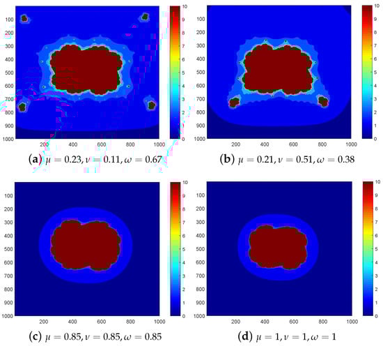 Figure 1. sets of with .
 - In Figure 2, the polynomial and is considered. We have comparable shapes, but the colors differ significantly. Additionally, Figure 2a,b depict the disconnectivity of orbits of the sets, while Figure 2c,d exhibit connectivity among their orbits.
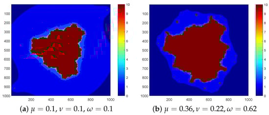
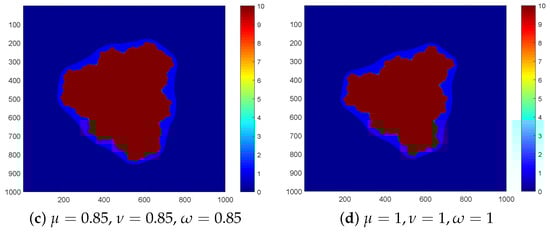 Figure 2. sets of with .
 - For Figure 3, the polynomial and is considered.
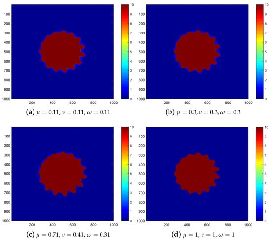 Figure 3. sets of with .
4.2. Generation of Sets in Picard–Ishikawa Iteration
We show quadratic, cubic, and higher-degree sets in a Picard–Ishikawa–type orbit for the complex polynomial .
- For Figure 4, the polynomial and is considered. We can observe that the shape in Figure 4a provides a disconnected set, while Figure 4b–d give connected sets. We can also observe that the lower the value of parameters is, the bigger the set shape changes. For and , the difference in shapes is significant.
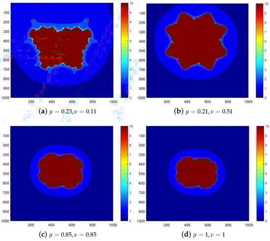 Figure 4. sets of of with .
 - For Figure 5, the polynomial and is considered. Although our shapes are identical, there is a significant color difference.
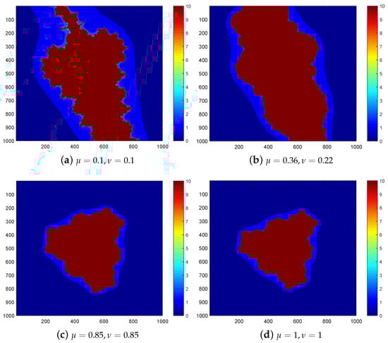 Figure 5. sets of of with .
 - In Figure 6, the polynomial and is considered.
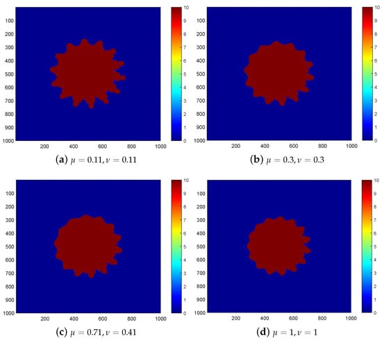 Figure 6. sets of of with .
5. Visualization of Sets
In this section, we delve into the visual representation of sets, showcasing their intricate structures. By manipulating the input parameters, we witness the emergence of vibrant colors and the transformation of the fractal’s shape, leading to a captivating visual experience.
For our exploration of sets, we utilize the escape criterion technique. The result of this process is the generation of two sets: one comprising points where the orbits remain bounded, forming the set, and the other consisting of points where the orbits escape to infinity, creating the background.
5.1. Generation of Sets
Algorithm 2 is the pseudocode for the creation of sets.
We show quadratic, cubic, and higher-degree sets in a Kalsoom at al.–type orbit for the complex polynomial .
- For Figure 7, we input and observe that the images are similar to a traditional set. The main body includes several bulbs of various sizes, but magnifying any picture bulb reveals the form of the entire image. All the sets in Figure 7 have downward faces and symmetry about the y-axis.
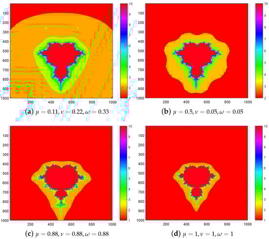 Figure 7. sets of with .
 - For Figure 8, we input , and it shows that each picture has two cardioids, two large bulbs, and four small bulbs and preserves symmetry about diagonals.
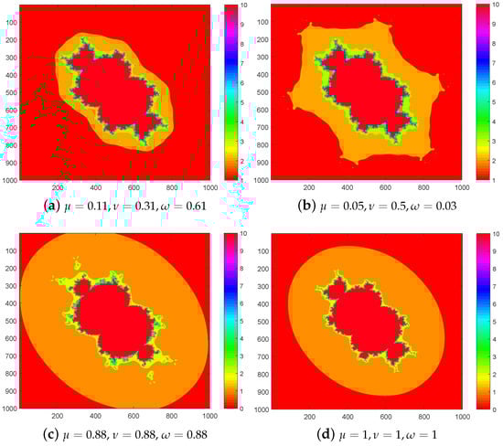 Figure 8. sets of with .
 - For Figure 9, we input , and we perceive that a clear color variation is involved. Figure 9c covers more area as compared with Figure 9d.
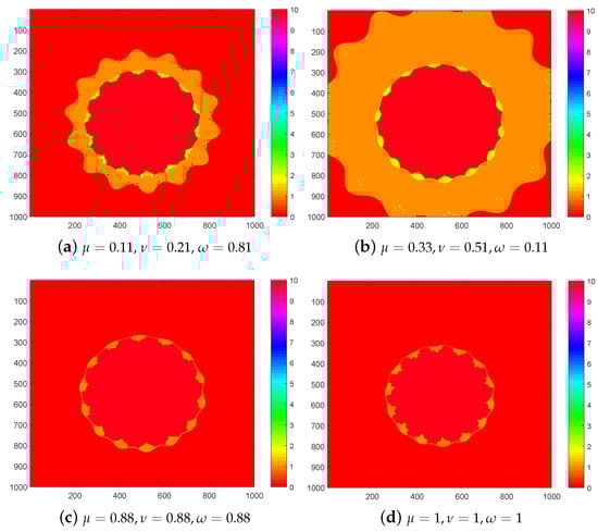 Figure 9. sets of with .
5.2. Generation of Sets in Picard–Ishikawa Iteration
We show quadratic, cubic, and higher-degree sets in a Picard–Ishikawa–type orbit for the complex polynomial .
- For Figure 10, we input and observe that the images are similar to a traditional set. The main body includes several bulbs of various sizes, but magnifying any picture bulb reveals the form of the entire image. Figure 10a–d have downward faces and symmetry about the y-axis. Notice that the pattern in Figure 10a is stretched and the bulb is broader, but the shapes in Figure 10c,d are compact and have a defined bulb.

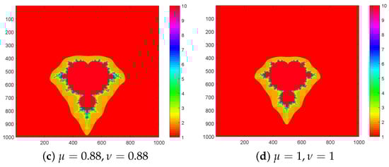 Figure 10. sets for with .
 - For Figure 11, we input , and it shows that each picture has two cardioids, two large bulbs, and four small bulbs and preserves symmetry along both diagonals.
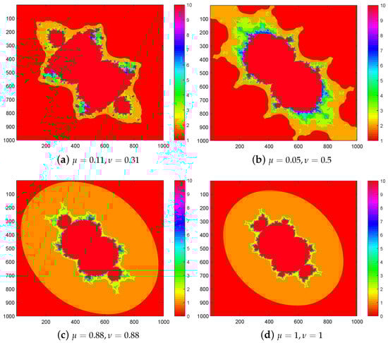 Figure 11. sets for with .
 - For Figure 12, we input , and we perceive that shapes are the same, but there is variability in colors. Figure 12c covers more area as compared with Figure 12d.
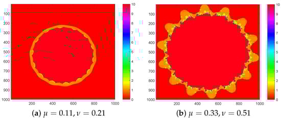
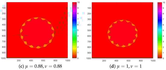 Figure 12. sets for with .
6. Discussion on the Sets Generated by Kalsoom et al. and Picard–Ishikawa Iteration Schemes
We have generated sets with Kalsoom et al. and Picard–Ishikawa iteration schemes. We checked the graphical behaviors of both iterations. For comparison, we took two sets, first, with Kalsoom et al. iteration and, second, with Picard–Ishikawa iteration and perceive that the results with Kalsoom et al. iteration are better than Picard–Ishikawa because they are in more compact form. For Figure 13a,b, we input the same area and the values of the parameters but obtained different results. Figure 13a shows that the shape of the set by using Kalsoom et al. iteration is compact with a defined bulb, and Figure 13b shows that the shape of the set by using Picard–Ishikawa iteration is stretched and the bulb is wider. The added value of the method presented in this research lies in the utilization of both Kalsoom et al. iteration and Picard–Ishikawa iteration. With Kalsoom et al. iteration, we achieve the shape of the traditional set even at lower values of the parameter. On the other hand, with Picard–Ishikawa iteration, we need to use higher values to obtain traditional sets.
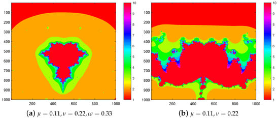
Figure 13.
.
7. Conclusions
In this article, different iteration processes and color maps have been employed to generate and sets. The utilization of these sets can be helpful to those interested in the automatic generation of visually appealing images. Escape criteria for the -degree polynomial to generate the said sets via Kalsoom et al. and Picard–Ishikawa iteration schemes with the polynomial have been proven. Additionally, new fractals for complex functions that are distinctly different from those introduced earlier have been obtained. Interesting and sets have been achieved by using different values of . A few examples of complex quadratic, cubic, and -degree polynomials have been presented. While the paper presents escape criteria that have proven effective in generating fractals, exploring alternative escape criteria could offer new perspectives on the generation process. Investigating different escape conditions and their impact on the resulting fractals could be a fascinating direction for future research. Moreover, this study can be extended to explore fractals beyond and sets. Investigating other fractal families, such as Multibrot sets, Biomorphs, or Barnsley fern, and applying the developed iterative procedures to generate and visualize these fractals would open new paths for further exploration in the field.
Open Problem: Can the results demonstrated in this paper be extended to include exponential and multivariate polynomials using any other iteration scheme?
Author Contributions
Each author equally contributed to writing and finalising the article. Conceptualization, A.T., M.R. and A.K.; methodology, A.T., M.R., A.K.; software, K.S.; validation, M.R. and D.K.A.; formal analysis, M.R. and D.K.A.; investigation, D.K.A.; resources, A.T. and D.K.A.; writing—original draft preparation, K.S.; writing—review and editing, D.K.A.; visualization, A.T.; supervision, A.T.; project administration, A.T. and A.K. All authors have read and agreed to the published version of the manuscript.
Funding
This research received no external funding.
Data Availability Statement
No new data was generated for this study.
Acknowledgments
The author extends the appreciation to the Deanship of Postgraduate Studies and Scientific Research at Majmaah University for funding this research work through project number (R-2024-1012).
Conflicts of Interest
The authors declare no conflicts of interest.
References
- Rassias, T.M. Topics in Polynomials: Extremal Problems, Inequalities, Zeros; World Scientific: Singapore, 1994. [Google Scholar]
- Rahman, Q.I.; Schmeisser, G. Analytic Theory of Polynomials (No. 26); Oxford University Press: Oxford, UK, 2002. [Google Scholar]
- Gardner, R.B.; Govil, N.K.; Milovanović, G.V. Extremal Problems and Inequalities of Markov-Bernstein Type for Algebraic Polynomials; Academic Press: Cambridge, MA, USA, 2022. [Google Scholar]
- Julia, G. Mémoire sur l’itération des fonctions rationnelles. J. Math. Pures Appl. 1918, 1, 47–245. [Google Scholar]
- Fatou, P. Sur les équations fonctionnelles. Bull. Soc. Math. Fr. 1919, 47, 161–271. [Google Scholar] [CrossRef]
- Mandelbrot, B.B.; Mandelbrot, B.B. The Fractal Geometry of Nature; WH Freeman: New York, NY, USA, 1982; Volume 1. [Google Scholar]
- Lakhtakia, A.; Varadan, V.V.; Messier, R.; Varadan, V.K. On the symmetries of the Julia sets for the process zp + c. J. Phys. A Math. Gen. 1987, 20, 3533. [Google Scholar] [CrossRef]
- Crowe, W.D.; Hasson, R.; Rippon, P.J.; Strain-Clark, P. On the structure of the Mandelbar set. Nonlinearity 1989, 2, 541. [Google Scholar] [CrossRef]
- Rochon, D. A generalized Mandelbrot set for bicomplex numbers. Fractals 2000, 8, 355–368. [Google Scholar] [CrossRef]
- Negi, A.; Rani, M. Midgets of superior Mandelbrot set. Chaos Solitons Fractals 2008, 36, 237–245. [Google Scholar] [CrossRef]
- Negi, A.; Rani, M. A new approach to dynamic noise on superior Mandelbrot set. Chaos Solitons Fractals 2008, 36, 1089–1096. [Google Scholar] [CrossRef]
- Devaney, R.L. A First Course in Chaotic Dynamical System: Theory and Experiment, 2nd ed.; Addison-Wesley: Boston, MA, USA, 1992. [Google Scholar]
- Lei, T. Similarity between the Mandelbrot set and Julia sets. Commun. Math. Phys. 1990, 134, 587–617. [Google Scholar] [CrossRef]
- Branner, B.; Hubbard, J.H. The iteration of cubic polynomials Part I: The global topology of parameter space. Acta Math. 1988, 160, 143–206. [Google Scholar] [CrossRef]
- Branner, B.; Hubbard, J.H. The iteration of cubic polynomials Part II: Patterns and parapatterns. Acta Math. 1992, 169, 229–325. [Google Scholar] [CrossRef]
- Geum, Y.H.; Hare, K.G. Groebner basis, resultants and the generalized Mandelbrot set. Chaos Solitons Fractals 2009, 42, 1016–1023. [Google Scholar] [CrossRef]
- Rani, M.; Kumar, V. Superior Julia set. Res. Math. Educ. 2004, 8, 261–277. [Google Scholar]
- Rani, M.; Kumar, V. Superior Mandelbrot set. Res. Math. Educ. 2004, 8, 279–291. [Google Scholar]
- Rana, R.; Chauhan, Y.S.; Negi, A. Non-linear dynamics of Ishikawa iteration. Int. J. Comput. Appl. 2010, 7, 43–49. [Google Scholar] [CrossRef]
- Chauhan, Y.S.; Rana, R.; Negi, A. New Julia sets of Ishikawa iterates. Int. J. Comput. Appl. 2010, 7, 34–42. [Google Scholar] [CrossRef]
- Rani, M.; Chugh, R. Julia sets and Mandelbrot sets in Noor orbit. Appl. Math. Comput. 2014, 228, 615–631. [Google Scholar]
- Kang, S.M.; Rafiq, A.; Latif, A.; Shahid, A.A.; Ali, F. Fractals through modified iteration scheme. Filomat 2016, 30, 3033–3046. [Google Scholar] [CrossRef][Green Version]
- Kang, S.M.; Rafiq, A.; Latif, A.; Shahid, A.A.; Kwun, Y.C. Tricorns and multicorns of-iteration scheme. J. Funct. Spaces 2015, 2015, 417167. [Google Scholar] [CrossRef]
- Kumari, M.; Ashish, R.C. New Julia and Mandelbrot sets for a new faster iterative process. Int. J. Pure Appl. Math. 2016, 107, 161–177. [Google Scholar] [CrossRef]
- Abbas, M.; Iqbal, H.; De la Sen, M. Generation of Julia and Madelbrot sets via fixed points. Symmetry 2020, 12, 86. [Google Scholar] [CrossRef]
- Kumari, S.; Gdawiec, K.; Nandal, A.; Postolache, M.; Chugh, R. A novel approach to generate Mandelbrot sets, Julia sets and biomorphs via viscosity approximation method. Chaos Solitons Fractals 2022, 163, 112540. [Google Scholar] [CrossRef]
- Kalsoom, A.; Rashid, M.; Sun, T.C.; Bibi, A.; Ghaffar, A.; Inc, M.; Aly, A.A. Fixed points of monotone total asymptotically nonexpansive mapping in hyperbolic space via new algorithm. J. Funct. Spaces 2021, 2021, 8482676. [Google Scholar] [CrossRef]
- Mann, W.R. Mean value methods in iteration. Proc. Am. Math. Soc. 1953, 4, 506–510. [Google Scholar] [CrossRef]
- Ishikawa, S. Fixed points by a new iteration method. Proc. Am. Math. Soc. 1974, 44, 147–150. [Google Scholar] [CrossRef]
- Noor, M.A. New approximation schemes for general variational inequalities. J. Math. Anal. Appl. 2000, 251, 217–229. [Google Scholar] [CrossRef]
- Agarwal, R.P.; Regan, D.O.; Sahu, D. Iterative construction of fixed points of nearly asymptotically nonexpansive mappings. J. Nonlinear Convex Anal. 2007, 8, 61. [Google Scholar]
- Barnsely, M. Fractals Everywhere, 2nd ed.; Academic Press: Cambridge, MA, USA, 1993. [Google Scholar]
- Liu, X.; Zhu, Z.; Wang, G.; Zhu, W. Composed accelerated escape time algorithm to construct the general Mandelbrot sets. Fractals 2001, 9, 149–153. [Google Scholar] [CrossRef]
- Tingen, L.L. The Julia and Mandelbrot Sets for the Hurwitz Zeta Function. Ph.D. Dissertation, University of North Carolina Wilmington, Wilmington, NC, USA, 2009. [Google Scholar]
- Strotov, V.V.; Smirnov, S.A.; Korepanov, S.E.; Cherpalkin, A.V. Object distance estimation algorithm for real-time fpga-based stereoscopic vision system. In Proceedings of the High-Performance Computing in Geoscience and Remote Sensing VIII, Berlin, Germany, 10–13 September 2018. [Google Scholar]
- Barrallo, J.; Jones, D.M. Coloring algorithms for dynamical systems in the complex plane. Vis. Math. 1999, 1, 4. [Google Scholar]
- Khatib, O. Real-Time Obstacle Avoidance for Manipulators and Mobile Robots; Springer: Berlin/Heidelberg, Germany, 1986. [Google Scholar]
- Kwun, Y.C.; Shahid, A.A.; Nazeer, W.; Abbas, M.; Kang, S.M. Fractal generation via CR iteration scheme with s-convexity. Inst. Electr. Electron. Eng. 2019, 7, 69986–69997. [Google Scholar] [CrossRef]


Disclaimer/Publisher’s Note: The statements, opinions and data contained in all publications are solely those of the individual author(s) and contributor(s) and not of MDPI and/or the editor(s). MDPI and/or the editor(s) disclaim responsibility for any injury to people or property resulting from any ideas, methods, instructions or products referred to in the content. |
© 2024 by the authors. Licensee MDPI, Basel, Switzerland. This article is an open access article distributed under the terms and conditions of the Creative Commons Attribution (CC BY) license (https://creativecommons.org/licenses/by/4.0/).