Machine Learning in Quasi-Newton Methods

Abstract

In this article, we consider the correction of metric matrices in quasi-Newton methods (QNM) from the perspective of machine learning theory. Based on training information for estimating the matrix of the second derivatives of a function, we formulate a quality functional and minimize it by using gradient machine learning algorithms. We demonstrate that this approach leads us to the well-known ways of updating metric matrices used in QNM. The learning algorithm for finding metric matrices performs minimization along a system of directions, the orthogonality of which determines the convergence rate of the learning process. The degree of learning vectors’ orthogonality can be increased both by choosing a QNM and by using additional orthogonalization methods. It has been shown theoretically that the orthogonality degree of learning vectors in the Broyden–Fletcher–Goldfarb–Shanno (BFGS) method is higher than in the Davidon–Fletcher–Powell (DFP) method, which determines the advantage of the BFGS method. In our paper, we discuss some orthogonalization techniques. One of them is to include iterations with orthogonalization or an exact one-dimensional descent. As a result, it is theoretically possible to detect the cumulative effect of reducing the optimization space on quadratic functions. Another way to increase the orthogonality degree of learning vectors at the initial stages of the QNM is a special choice of initial metric matrices. Our computational experiments on problems with a high degree of conditionality have confirmed the stated theoretical assumptions.

1. Introduction

The problem of unconstrained minimization of smooth functions in a finite-dimensional Euclidean space has received a lot of attention in the literature [1,2]. In unconstrained optimization, in contrast to constrained optimization [3], the process of optimizing the objective function is carried out in the absence of restrictions on variables. Unconstrained problems arise also as reformulations of constrained optimization problems, in which the constraints are replaced by penalization terms in the objective function that have the effect of discouraging constraint violations [2].

Well-known methods [1,2] that enable us to solve such a problem include the gradient method, which is based on the idea of function local linear approximation, or Newton’s method, which uses its quadratic approximation. The Levenberg–Marquardt method is a modification of Newton’s method, where the direction of descent differs from that specified by Newton’s method. The conjugate gradient method is a two-step method in which the parameters are found from the solution of a two-dimensional optimization problem.

Quasi-Newton minimization methods are effective tools of solving smooth minimization problems when the function level curves have a high degree of elongation [4,5,6,7]. QNMs are commonly applied in a wide range of areas, such as biology [8], image processing [9], technics [10,11,12,13,14,15], and deep learning [16,17,18].

The QNM is based on the idea of using a matrix of second derivatives reconstructed from the gradients of a function. The first QNM was proposed in [19] and improved in [20]. The generally accepted notation for the matrix updating formula in this method is DFP. Nowadays, there are a significant number of equations for updating matrices in the QNM [4,5,6,7,21,22,23,24,25,26,27,28], and it is generally accepted [4,5] that among a variety of QNMs, the best methods use the BFGS matrix updating equation [29,30,31]. However, it has been experimentally established, but not theoretically explained, why the BFGS generates the best results among the QNMs [5].

A sampled version of the BFGS method named limited-memory BFGS (L-BFGS) [32] was presented to handle high-dimensional problems. The algorithm stores only a few vectors that represent the approximation of the Hessian instead of the entire matrix. A version with bound constraints was proposed in [33].

The penalty method [2] was developed for solving constrained optimization problems. The unconstrained problems are formed by adding a term, called a penalty function, to the objective function. The penalty is zero for feasible points and non-zero for infeasible points.

The development of QNMs occurred spontaneously through the search for matrix updating equations that satisfy certain properties of data approximation obtained in the problem solving process. In this paper, we consider a method for deriving matrix updating equations in QNMs by forming a quality functional based on learning relations for matrices, followed by obtaining matrix updating equations in the form of a step of the gradient method for minimizing the quality functional. This approach has shown high efficiency in organizing subgradient minimization methods [34,35].

In machine learning theory, the system in which the average risk (mathematical expectation of the total loss function) is minimal is considered optimal [36,37]. The goal of learning represents the state that has to be reached by the learning system in the process of learning. The selection of such a desired state is actually achieved by a proper choice of a certain functional that has an extremum which corresponds to the desired state [38]. Thus, in the matrix learning process, it is necessary to formulate a quality functional.

In QNMs, for each of the matrix rows, there is a product of the vector which exists as a learning relation. Consequently, we have a linear model with the coefficients of the matrix row as its parameters. Thus, we may formulate a quadratic learning quality functional for a linear model and obtain a gradient machine learning (ML) algorithm. This paper shows how one can obtain known methods for updating matrices in QNMs based on a gradient learning algorithm. Based on the general properties of convergence of gradient learning algorithms, it seems relevant to study the origins of the effectiveness of metric updating equations in QNMs.

In a gradient learning algorithm, the sequence of steps is represented as a method of minimization along a system of directions. The degree of orthogonality of these directions determines the convergence rate of the algorithm. The use of gradient learning algorithms for deriving matrix updating equations in QNMs enables us to analyze the quality of matrix updating algorithms based on the convergence rate properties of the learning algorithms. This paper shows that the higher degree of orthogonality of learning vectors in the BFGS method determines its advantage compared to the DFP method.

Studies on quadratic functions identify conditions under which the space dimension is reduced during the QNM iterations. The dimension of the minimization space is reduced when the QNM includes iterations with an exact one-dimensional descent or an iteration with additional orthogonalization. It is possible to increase the orthogonality of the learning vectors and thereby increase the convergence rate of the method through special normalization of the initial matrix.

The computational experiment was carried out on functions with a high degree of conditionality. Various ways of increasing the orthogonality of learning vectors were assessed. The theoretically predicted effects of increasing the efficiency of QNMs confirmed their effectiveness in practice. It turned out that with an approximate one-dimensional descent, additional orthogonalization in iterations of the algorithm significantly increased the efficiency of the method. In addition, the efficiency of the method also increased significantly with the correct normalization of the initial matrix.

The rest of this paper is organized as follows. In Section 2, we provide basic information about matrix learning algorithms in QNMs. Section 3 contains an analysis of matrix updating formulas in QNMs. A symmetric positive definite metric is considered in Section 4. Section 5 gives a qualitative analysis of the BFGS and DFP matrix updating equations. Methods for reducing the minimization space of QNMs on quadratic functions are presented in Section 6. Methods for increasing the orthogonality of learning vectors in QNMs are considered in Section 7. In Section 8, we present a numerical study, and the last section summarizes the work.

2. Matrix Learning Algorithms in Quasi-Newton Methods

Consider the minimization problem

f(x) → min, x ∈ Rⁿ.

The QNM for this problem is iterated as follows:

$$x_{}^{k+1}=x_{}^k+{\beta }_k{s}_{}^k,s_{}^k=-H_{}^k\nabla f\left(x_{}^k\right),$$

(1)

$${\beta }_k=\underset{\beta \ge 0}{\arg \min }f\left(x^k+\beta s^k\right),$$

(2)

$$\mathsf{\Delta }{x}_{}^k=x_{}^{k+1}-x_{}^k,y_{}^k=\nabla f\left(x_{}^{k+1}\right)-\nabla f\left(x_{}^k\right),$$

(3)

$$H_{}^{k+1}=H\left(H_{}^k,\mathsf{\Delta }{x}_{}^k,y_{}^k\right).$$

(4)

Here, $\nabla f\left(x\right)$ is the gradient of a function, s^k is the search direction, and β_k is chosen to satisfy the Wolfe conditions [2]. Further, $H^k\in R^{n\times n}$ is a symmetric matrix which is used as an approximation of the Hessian inverse. The operator

$$H\left(H,\mathsf{\Delta }x,y\right)\in R^{n\times n},H\in R^{n\times n},\mathsf{\Delta }x,y\in R^n$$

(5)

specifies a certain equation for updating the initial matrix H. At the input of the algorithm, the starting point x₀ and the symmetric strictly positive definite matrix H⁰ must be specified. Such a matrix will be denoted as H⁰ > 0.

Let us consider the relations for obtaining updating equations for H^k matrices on quadratic functions:

$$f\left(x\right)=\frac{1}{2}⟨x-x_{}^{*},A(x-x_{}^{*})⟩+d,A>0,$$

(6)

where x* is the minimum point. Here and below, the expression <·,·> means a scalar product of vectors. Without a loss of generality, we assume d = 0. The gradient of a quadratic function f(x) is ∇f(x) = A(x − x*). For Δx ∈ Rⁿ, the gradient difference y = ∇f(x + Δx) − ∇f(x) satisfies the relation:

$$A\mathsf{\Delta }x=y\mathrm{or}{A}^{-1}y=\mathsf{\Delta }x.$$

(7)

The equalities in (7) are used to obtain various equations for updating matrices H^k, which are approximations for A⁻¹, or matrices B^k = (H^k)⁻¹, which are approximations for A. An arbitrary equation for updating matrices H or B, the result of which is a matrix satisfying (7), will be denoted by H(H, Δx, y) or B(B, Δx, y), respectively.

Denoting as A_i and A_i⁻¹ rows of the corresponding matrices A and A⁻¹ with i-th index, then, according to (7), we obtain equations for the learning relations necessary to formulate algorithms for matrix rows’ learning:

$$A_i\mathsf{\Delta }x=y_i,A_i^{-1}y=\mathsf{\Delta }{x}_i,i=\mathrm{1,2},\dots ,n,$$

(8)

where y_i and Δx_i are the components of the vectors in (7). The relations in (8) make it possible to use machine learning algorithms of a linear model in the parameters to estimate the rows of the corresponding matrices.

Let us formulate the problem of estimating the parameters of a linear model from observational data.

ML problem: find unknown parameters c* ∈ Rⁿ of the linear model

$$y=⟨z,c⟩,z,c\in R^n,y\in R^1$$

(9)

from observational data

$$y_k\in R^1,{\mathrm{z}}_{}^k\in R^n,k=\mathrm{0,1},2,\dots ,$$

(10)

where y_k = <c*, z^k>. We will use an indicator of training quality,

$$Q(z,c)=\frac{1}{2}{(〈z,c〉-y)}^2,$$

(11)

which is an estimate of the quality functional required to find c*.

Function (11) is a loss function. Due to the large dimension of the problem of estimating the elements of metric matrices, the use of the classical least squares method becomes difficult. We use the adaptive least squares method (recurrent least squares formulas).

The gradient learning algorithm based on (11) has the following form:

$$c_{}^{k+1}=c_{}^k-h_k\nabla Q(z_{}^k,c_{}^k)=c_{}^k-h_k(⟨z_{}^k,c_{}^k⟩-y_k)z_{}^k.$$

(12)

Due to the orthogonality of the training vectors, the stochastic gradient method in the form “receiving of an observation-training-forgetting the observation information” in quasi-Newton methods enables us to obtain good approximations of the inverse matrices of second derivatives while maintaining their symmetry and positive definiteness.

In this paper, the value of such consideration is that we are able to identify the advantages of the BFGS method and obtain a method with orthogonalization of learning vectors and prove these provisions through testing.

The Kaczmarz algorithm [39] is a special case of (12) with the form

$$c_{}^{k+1}=c_{}^k-\frac{(⟨z_{}^k,c_{}^k⟩-y_k)}{⟨z_{}^k,c_{}^k⟩}{z}_{}^k.$$

(13)

Let us list some of the properties of process (13), which we use to justify the properties of matrix updating in QNMs.

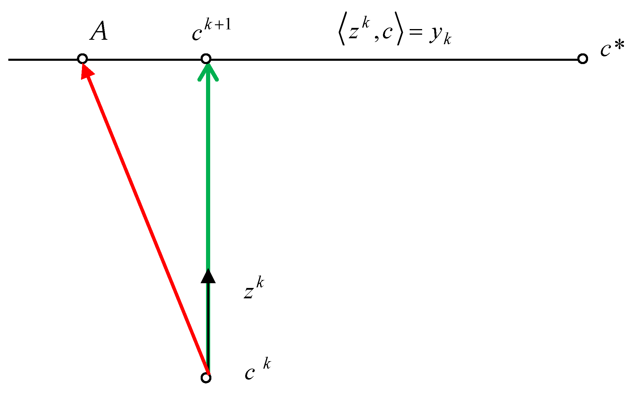
Property 1.

Process (13) ensures the equality

$$y_k=⟨z_{}^k,c_{}^{k+1}⟩,$$

(14)

and the solution is achieved under the condition of minimum changes in the parameters’ values $\Vert c_{}^{k+1}-c_{}^k\Vert$.

Property 2.

If y_k = <c*, z^k> then the iteration of process (13) is equivalent to the step of minimizing the quadratic function

$$\varphi \left(c\right)=⟨c-c^{*},c-c^{*}⟩/2$$

(15)

from the point c^k along the direction z^k.

Proof. 

Property 2 is justified by the direct implementation of the function in (15) which is the minimizing step along the direction z^k, which is presented in Figure 1. Property 1 follows from the fact that movement to the point c^k+1 is carried out along the normal to the hyperplane <z^k, c> = y_k, that is, along the shortest path (Figure 1). Movement to other points on the hyperplane, for example to point A, satisfy only the condition in (14). □

Let us denote the residual as r^k = c^k − c*. By subtracting c* from both sides of (13) and making transformations, we obtain the following learning algorithm in the form of residuals:

$$r_{}^{k+1}=W\left(z_{}^k\right)r_{}^k,W(z)=I-\frac{z{z}^T}{z^{T}z},$$

(16)

where I is the identity matrix. The sequence of minimization steps can be represented in the form of the residual transformation, where m is the number of iterations:

$$r_{}^{k+1}=W_{k-m}^k(z)r_{}^{k-m},W_{k-m}^k\left(z\right)=W\left(z_{}^k\right)W(z_{}^{k-1})\cdots W(z_{}^{k-m}).$$

(17)

The convergence rate of process (13) is significantly affected by the degree of orthogonality of the learning vectors z. The following property reflects the well-known fact of the minimization algorithm termination along orthogonal directions of the quadratic form of (15) with equal Hessian eigenvalues.

Property 3.

Let vectors z^k, k = l, l + 1,…, l + n − 1 for a sequence of n iterations (13) be mutually orthogonal. Then, the solution c* minimizing the function (15) is obtained in no more than n steps of the process (13) for an arbitrary initial $c_l$, wherein

$$r_{}^{l+n}=W_l^{l+n-1}(z)r_{}^l=0,W_l^{l+n-1}(z)=0.$$

(18)

The following results are useful to estimate the convergence rate of the process in (13) as a method for minimizing the function in (15) without orthogonality of the descent vectors.

Consider a cycle of iterations for minimizing a function θ(x), x ∈ Rⁿ, along the column vectors z^k, ‖z^k‖ = 1, k = 1,…, n, of matrix Z ∈ R^n×n:

$$x_{k+1}=x_k+{\beta }_k{z}_k,{\beta }_k=\underset{\beta \ge 0}{\arg \min }\theta \left(x_k+\beta z_k\right),k=1,\dots ,n.$$

(19)

Here and below, we will use the Euclidean vector norm ‖x‖ = <x, x>^1/2. Let us present the result of the iterations in (19) in the form of the operator x_n+1 = XP(x₁, Z). Consider the process

$$u^{q+1}=XP(u^q,Z^q),q=\mathrm{0,1},\dots .,$$

(20)

where matrices Z^q and the initial approximation u⁰ are given. To estimate the convergence rate of the QNM and the convergence rate of the metric matrix approximation, we need the following assumption about the properties of the function.

Assumption 1.

Let the function be strongly convex, with a constant ρ > 0, and differentiable, and its gradient satisfy the Lipschitz condition with a constant L > 0.

We assume that the function f(x), x ∈ Rⁿ, is differentiable and strongly convex in Rⁿ, i.e., there exists ρ > 0 such that for all x,y ∈ Rⁿ and α ∈ [0, 1], the inequality holds,

$$f\left(\alpha x+\left(1-\alpha \right)y\right)\le \alpha f(x)+(1-\alpha )f(y)-\alpha (1-\alpha )\rho {‖x-y‖}^2/2,$$

and its gradient ∇f(x) satisfies the Lipschitz condition:

$$‖\nabla f(x)-\nabla f(y)‖\le L‖x-y‖\forall x,y\in R^n,L>0.$$

(21)

Let us denote the minimum point of the function θ(x) by x*. The following theorem [40] establishes the convergence rate of the iteration cycle (20).

Theorem 1.

Let the function θ(x), x ∈ Rⁿ, satisfy Assumption 1; let matrices Z^q of the process in (20) be such that minimum eigenvalues μ ^q of matrices (Z^q)^T Z^q satisfy the constraint μ ^q ≥ μ₀ > 0. Then, the following inequality estimates the convergence rate of the process in (20):

$$\theta (u^m)-\theta (x*)\le [\theta (u^0)-\theta (x*)]\exp \left(-\frac{m{\rho }^2{\mu }_0^2}{2L^2{n}^3}\right).$$

(22)

Estimate (22) enables us to formulate the following property of the process in (13).

Property 4.

Let vectors z_k, k = 1,…,n−1, be given in (13), the columns of the matrices Z be composed of vectors z_k/‖z_k‖, and the minimum eigenvalue μ of the matrix Z^T Z satisfy the constraint μ ≥ μ₀ > 0. Then, the following inequality estimates the convergence rate:

$$\Vert c_{}^n-c^{*}{\Vert }^2\le \Vert c_{}^0-c^{*}{\Vert }^2\exp \left(-\frac{{\mu }_0^2}{2n^3}\right).$$

(23)

Proof. 

Let us apply the results of Theorem 1 to the process in (13). The strong convexity and Lipschitz constants for the gradient of the quadratic function in (15) are the same: ρ = L = 1. Using Property 2 and the estimate in (22) for m = 1, we obtain (23). □

The property of operators $W_l^{l+n-1}$, when the conditions of Property 4 are met, is determined by the estimate in (23), which can be represented in the following form:

$$r_{}^n=\Vert W_0^{n-1}(z)r_{}^0{\Vert }^2\le \Vert r_{}^0{\Vert }^2\exp \left(-\frac{{\mu }_0^2}{2n^3}\right)$$

(24)

Thus, the Kaczmarz algorithm provides a solution to the equality in (14) for the last observation, while it implements a local learning strategy, i.e., a strategy for iteratively improving the approximation quality from a functional (15) point of view. If the learning vectors are orthogonal, the solution is found in no more than n iterations. When n learning vectors are linearly independent, the convergence rate (23) is determined by the degree of the learning vectors’ orthogonality. The degree of the vectors’ orthogonality will indicate the boundedness of the minimum eigenvalue μ ≥ μ₀ > 0 of the matrix Z^TZ defined in Property 4.

Using the learning relations in (8), we obtain machine learning algorithms for estimating the rows of the corresponding matrices in the form of the process in (13). Consequently, the question of analyzing the quality of algorithms for updating matrices in QNMs will consist of analyzing learning relations like (8) and the degree of orthogonality of the vectors involved in training.

3. Gradient Learning Algorithms for Deriving and Analyzing Matrix Updating Equations in Quasi-Newton Methods

Well-known equations for matrix updating in QNMs were found as equations that eliminate mismatch on a new portion of training information. In machine learning theory, a quality measure is formulated. A gradient minimization algorithm is used to minimize this measure. Our goal is to give an account of QNMs from the standpoint of machine learning theory, i.e., to formulate quality measures of training and construct their minimization algorithms. This approach enables us to obtain a unified method for deriving matrix updating equations and extend the known facts and algorithms of learning theory to solve analysis of and achieve improvement in QNMs.

Let us obtain formulas for updating matrices in QNMs using the quadratic model of the minimized function in (6) and learning relations in (7). For one of the learning relations in (7), we present a complete study of Properties 1–4.

Let the current approximation H of the matrix H* = A⁻¹ be known. It is required to construct a new approximation using the learning relations in (7) for the rows of the matrix in (8):

$$H^{*}y=\Delta x\mathrm{or}{H}_i^{*}y=\Delta x_i^{},i=1,2,\dots ,n.$$

(25)

To evaluate each row of the matrix H* based on (25), we apply Algorithm (13). As a result, we obtain the following matrix updating equation:

$$H_{}^{+}=H_{B2}(H,\mathsf{\Delta }x,y)=H+\frac{\left(\mathsf{\Delta }x-Hy\right)y^T}{y^{T}y},$$

(26)

which is known as the 2nd Broyden method for estimating matrices when solving systems of non-linear equations [5,6].

Equation (26) determines the step of minimizing a type of functional of (15) for each of the rows H_i of matrix H along the direction y:

$$\varphi \left(H_i\right)=\Vert H_i-H_i^{*}{\Vert }^2/2,i=1,2,\dots ,n.$$

(27)

The matrix residual is R = H − H*. Because of the iteration of (26), the residual is transformed according to the rule

$$R_{}^{+}=RW\left(y\right).$$

(28)

Let us denote the scalar product for matrices A,B ∈ $R^{n\times n}$ as

$$〈A,B〉={\displaystyle \sum _{i=1}^n{A}_i^T{B}_i^{}}={\displaystyle \sum _{j=1}^n{\displaystyle \sum _{i=1}^n{A}_{ij}^{}{B}_{ij}^{}}}.$$

We use the Frobenius norm of matrices:

$$\Vert H\Vert ={\left({\displaystyle \sum _{i=1}^n\Vert H_i^{}{\Vert }^2}\right)}^{1/2}.$$

Let us define the function,

$$\Phi (H)={\sum }_{i=1}^n\Vert H_i-H_i^{*}{\Vert }^2/2=\Vert H-H_{}^{*}{\Vert }^2/2,$$

(29)

and reformulate Properties 1–4 for the matrix updating process in (26).

Theorem 2.

Iteration (26) is equivalent to the minimization step Φ(H) from a point H along the direction ΔH:

$$\Delta H=\left(\Delta x-Hy\right)y^T/y^{T}y,$$

(30)

where

$$H_{}^{+}y=\Delta x$$

(31)

$$\Vert H_{}^{+}-H\Vert \le \Vert H_{}^{\Delta x}-H\Vert$$

(32)

for arbitrary matrices $H^{\Delta x}\in R^{n\times n}$ satisfying the condition in (31).

Proof of Theorem 2.

Let us show that the condition for the minimum of the function in (27) along the direction ΔH (30) is satisfied at the point $H^{+}$:

$$\begin{array}{ll}⟨\mathsf{\Delta }H,\nabla \Phi \left(H_{}^{+}\right)⟩& ={\displaystyle \sum _{j=1}^n}{\displaystyle \sum _{i=1}^n}(\mathsf{\Delta }x-Hy{)}_i{y}_j(H_{ij}^{+}-H_{ij}^{*})\\ & ={\displaystyle \sum _{i=1}^n}(\mathsf{\Delta }x-Hy{)}_i(H_i^{+}-H_i^{*})y={\displaystyle \sum _{i=1}^n}(\mathsf{\Delta }x-Hy{)}_i(\mathsf{\Delta }{x}_i-\mathsf{\Delta }{x}_i)=0.\end{array}$$

(33)

 □

Next, we prove (32) by showing that ΔH is the normal of the hyperplane of matrices satisfying the condition in (31). To do this, we prove orthogonality of the vector in (30) to an arbitrary vector of the hyperplane, formed as the difference of matrices belonging to the hyperplane V = H¹ − H²:

$$\begin{array}{ll}⟨\mathsf{\Delta }H,H_{}^1-H_{}^2)⟩& ={\displaystyle \sum _{j=1}^n}{\displaystyle \sum _{i=1}^n}(\mathsf{\Delta }x-Hy{)}_i{y}_j(H_{ij}^1-H_{ij}^2)\\ & ={\displaystyle \sum _{i=1}^n}(\mathsf{\Delta }x-Hy{)}_i(H_i^1-H_i^2)y={\displaystyle \sum _{i=1}^n}(\mathsf{\Delta }x-Hy{)}_i(\mathsf{\Delta }{x}_i-\mathsf{\Delta }{x}_i)=0.\end{array}$$

Let us prove an analogue of Property 3 for (26).

Theorem 3.

Let the vectors y_k, k = l, l + 1, …, l + n − 1, for the sequence of n iterations in (26) be mutually orthogonal, then the solution H* to the minimization problem in (29) will be obtained in no more than n steps of the process in (26),

$$H_{}^{k+1}=H_{B2}(H_{}^k,\Delta x_k,y_k),k=l,l+1,\dots ,l+n-1,$$

(34)

for an arbitrary matrix H^l,

$$R_{}^{l+n}=R_{}^{l+n}\left[W_l^{l+n-1}\right(y){]}^T=0.$$

(35)

Proof of Theorem 3.

From (28), the orthogonality of vectors y_k and (18) follows (35). □

Theorem 4.

Let vectors y_k, k = 0, 1, …, n − 1, in (13) be given, vectors y_k/‖y_k‖ be columns of matrix P, and the minimum eigenvalue μ of a matrix P^TP satisfy the constraint μ ≥ μ₀ > 0. Then, to estimate the convergence rate of the process in (34), the following inequality holds:

$$\Vert H_{}^n-H_{}^{*}{\Vert }_{}^2\le \Vert H_{}^0-H_{}^{*}{\Vert }_{}^2\exp \left(-\frac{{\mu }_0^2}{2n^3}\right).$$

(36)

Proof of Theorem 4.

According to Property 4 and conditions of the theorem, the rows of matrices will have the following estimates (23):

$$\Vert H_i^n-H_i^{*}{\Vert }_{}^2\le \Vert H_i^0-H_i^{*}{\Vert }_{}^2\exp \left(-\frac{{\mu }_0^2}{2n^3}\right),i=\mathrm{0,1},\dots ,n-1.$$

A similar inequality will be true for the sums of the left and right sides. Considering the connection between the norms $\Vert H_{}^n-H_{}^{*}{\Vert }_{}^2={\sum }_{i=1}^n\Vert H_i^n-H_i^{*}{\Vert }_{}^2$, we obtain the estimate in (36). □

In the case when the matrix H is symmetric, two products of the matrix H* and the vector y are known:

$$H_{}^{*}y=\mathsf{\Delta }x,y_{}^T{H}_{}^{*}=\mathsf{\Delta }{x}_{}^T.$$

(37)

Applying the process in (28) twice for (37), we obtain a new process for updating the matrix residual:

$$R_{}^{+}=W\left(y\right)RW\left(y\right).$$

(38)

Expanding (38), we obtain the updating formula $H^{+}=H_G(H,\Delta x,y)$ of J. Grinstadt [5,6], where

$$H_G(H,\Delta x,y)=H+\frac{〈Hy-\Delta x,y〉y{y}^T}{{〈y,y〉}^2}-\frac{y{\left(Hy-\Delta x\right)}^T+\left(Hy-\Delta x\right)y^T}{〈y,y〉}.$$

(39)

Let us reformulate Properties 1–4 of the matrix updating process (26) for (39).

Theorem 5.

The iteration of (39) is equivalent to the minimization step Φ(H) from a point H along the $\Delta H$ direction:

$$\Delta H=\frac{〈Hy-\Delta x,y〉y{y}^T}{{\left(y^{T}y\right)}^2}-\frac{y{\left(Hy-\Delta x\right)}^T}{y^{T}y}-\frac{\left(Hy-\Delta x\right)y^T}{y^{T}y}.$$

(40)

At the same time,

$$H_{}^{+}y=\Delta x,y_{}^T{H}_{}^{+}=\Delta x_{}^T,$$

(41)

$$\Vert H_{}^{+}-H\Vert \le \Vert H_{}^{\Delta x}-H\Vert$$

(42)

for arbitrary matrices $H^{\Delta x}\in R^{n\times n}$ satisfying the condition in (41).

Proof of Theorem 5.

Let us show that at the point $H_{}^{+}$, the condition for the minimum of the function in (27) along the direction ΔH is satisfied:

$$⟨\mathsf{\Delta }H,\nabla \Phi \left(H_{}^{+}\right)⟩=⟨\mathsf{\Delta }H,H_{}^{+}-H_{}^{*}⟩=0.$$

(43)

In (43), let us consider the scalar product for each term of (40) separately. The third term of Expression (40) coincides with (30). The equality to zero of the scalar product for it was obtained in (33). For the first term, the calculations are similar to (33):

$$\begin{array}{l}⟨\mathsf{\Delta }{H}_{}^1,\nabla \Phi \left(H_{}^{+}\right)⟩=\frac{〈Hy-\mathsf{\Delta }x,y〉}{{〈y,y〉}^2}{\displaystyle \sum _{j=1}^n}{\displaystyle \sum _{i=1}^n}{y}_i{y}_j(H_{ij}^{+}-H_{ij}^{*})\\ =\frac{〈Hy-\mathsf{\Delta }x,y〉}{{〈y,y〉}^2}{\sum }_{i=1}^n{y}_i(H_i^{+}-H_i^{*})y=\frac{〈Hy-\mathsf{\Delta }x,y〉}{{〈y,y〉}^2}{\sum }_{i=1}^n{y}_i(\mathsf{\Delta }{x}_i-\mathsf{\Delta }{x}_i)=0.\end{array}$$

Let us carry out calculations for the second term using the symmetry of matrices:

$$\begin{array}{l}〈y,y〉⟨\mathsf{\Delta }{H}_{}^2,\nabla \Phi \left(H_{}^{+}\right)⟩={\sum }_{j=1}^n{\sum }_{i=1}^n{y}_i(Hy-\mathsf{\Delta }x{)}_j(H_{ij}^{+}-H_{ij}^{*})\\ ={\sum }_{j=1}^n(Hy-\mathsf{\Delta }x{)}_j{\sum }_{i=1}^n{y}_i\left(H_{ij}^{+}-H_{ij}^{*}\right)={\sum }_{j=1}^n(Hy-\mathsf{\Delta }x{)}_j(H_j^{+}-H_j^{*})y\\ ={\sum }_{j=1}^n(Hy-\mathsf{\Delta }x{)}_j(\mathsf{\Delta }{x}_j-\mathsf{\Delta }{x}_j)=0.\end{array}$$

Proof (43) is complete. Next, we prove that ΔH is the normal of the hyperplane of matrices satisfying the condition in (42). To do this, we prove that the vector ΔH is orthogonal to an arbitrary vector of the hyperplane, formed as the difference of matrices belonging to the hyperplane $V=H^1-H^2$, that is, <ΔH, $H^1-H^2$ > = 0. Since the matrices $H^1$ and $H^2$ satisfy the condition in (42), the proof is identical to the justification of the equality in (43). □

The following theorem establishes the convergence rate for a series of successive updates (39).

Theorem 6.

Let vectors y_k, k = l, l + 1, …, l + n − 1, for the sequence of n iterations of (39) be mutually orthogonal. Then, the solution to the minimization problem in (29) can be obtained in no more than n steps of the process in (39),

$$H^{k+1}=H_G(H^k,\Delta x_k,y_k),k=l,l+1,\dots ,l+n-1,$$

(44)

for an arbitrary symmetric matrix $H^l$:

$$R^{l+n}=W_l^{l+n-1}(y)R^{l+n}{[W_l^{l+n-1}(y)]}^T=0.$$

(45)

Proof of Theorem 6.

The update in (45) can be represented as two successive multiplications by $W_l^{l+n-1}(y)$, first from the left and then from the right. For each of the updates, the estimate in (35) is valid. □

Theorem 7.

Let vectors y_k, k = 0, 1, …, n − 1, be given, vectors y_k/‖y_k‖ be columns of matrix P, and the minimum eigenvalue μ of a matrix P^TP satisfy the constraint μ ≥ μ₀ > 0. Then, to estimate the convergence rate of the process in (44), the following inequality holds:

$${\Vert H^n-H^{*}\Vert }^2\le {\Vert H^0-H^{*}\Vert }^2\exp \left(-\frac{{\mu }_0^2}{n^3}\right).$$

(46)

Proof of Theorem 7.

The matrix residual is updated according to the rule

$$R^{l+n}=W_l^{l+n-1}(y)R^{l+n}{[W_l^{l+n-1}(y)]}^T,$$

which can be represented as two successive multiplications by $W_l^{l+n-1}(y)$, first from the left and then from the right. The estimate in (36) is valid for each of the updates, which proves (46). □

4. Symmetric Positive Definite Metric and Its Analysis

Let Function (6) be quadratic. We use the coordinate transformation

$$\widehat{x}=Vx.$$

(47)

Let the matrix V satisfy the relation

$$V^{\mathrm{T}}V={\nabla }^{2}f\left(x\right)=A.$$

(48)

In the new coordinate system, the minimized function takes the following form:

$$\widehat{f}(\widehat{x})=f\left(V^{-1}\widehat{x}\right)=f(x).$$

(49)

Quadratic Function (6), considering (49), (47), and (48), takes the following form:

$$\widehat{f}(\widehat{x})=\frac{1}{2}(\widehat{x}-{\widehat{x}}^{*}{)}^T{V}^{-T}A{V}^{-1}(\widehat{x}-{\widehat{x}}^{*})=\frac{1}{2}〈\widehat{x}-{\widehat{x}}^{*},\widehat{x}-{\widehat{x}}^{*}〉.$$

(50)

Here, ${\widehat{x}}^{\mathrm{*}}$ is the minimum point of the function. According to (38) and (50), the matrix of second derivatives is the identity matrix ${\nabla }^2\widehat{f}(\widehat{x})=I$. Let us denote $\widehat{r}=\widehat{x}-{\widehat{x}}^{*}$. The gradient is

$$\nabla \widehat{f}(\widehat{x})=r(\widehat{x})=\widehat{r}=\widehat{x}-{\widehat{x}}^{*}.$$

(51)

For the characteristics of functions $\widehat{f}(\widehat{x})$ and f(x), the following relationships are valid:

$$\nabla \widehat{f}(\widehat{x})=V^{-T}\nabla f(x),{\nabla }^2\widehat{f}(\widehat{x})=V^{-T}{\nabla }^{2}f(x)V^{-1},$$

(52)

$$\mathsf{\Delta }\widehat{x}={\widehat{x}}_{}^{+}-\widehat{x}=V{x}_{}^{+}-Vx=V\mathsf{\Delta }x,$$

(53)

$$\widehat{y}=\nabla \widehat{f}\left(x^{+}\right)-\nabla \widehat{f}\left(x\right)=V^{-T}f\left(x^{+}\right)-V^{-T}f\left(x\right)=V^{-T}y$$

(54)

where notation $V^{-\mathrm{T}}={\left(V^{\mathrm{T}}\right)}^{-1}$ is used.

From (53), (54), and the properties of matrices V (48), the following equality holds:

$$\widehat{y}=\Delta \widehat{x}\equiv z$$

(55)

For the symmetric matrix $\widehat{H}$, two products of the matrix ${\widehat{H}}^{*}$ and the vector y are known:

$${\widehat{H}}_{}^{*}\widehat{y}=\Delta \widehat{x},{\widehat{y}}_{}^T{\widehat{H}}_{}^{*}=\Delta {\widehat{x}}_{}^T.$$

(56)

Applying the process in (28) twice to (56), we obtain a new process for updating the matrix residual $\widehat{R}=\widehat{H}-I$:

$${\widehat{R}}_{}^{+}=W(\widehat{y})\widehat{R}W(\widehat{y})=W(z)\widehat{R}W(z).$$

(57)

Taking into account (55), the update in (39) takes the form

$${\widehat{H}}_{BFGS}^{+}={\widehat{H}}_G\left(\widehat{H},\mathsf{\Delta }\widehat{x},\widehat{y}\right)=\widehat{H}+\frac{〈\widehat{H}z-z,z〉z{z}^T}{{〈z,z〉}^2}-\frac{z{\left(\widehat{H}z-z\right)}^T+\left(\widehat{H}z-z\right)z^T}{〈z,z〉}.$$

(58)

Let us consider the methods in (1)–(4) in relation to the function $\widehat{f}(\widehat{x})$ in the new coordinate system.

$${\widehat{x}}_{}^{k+1}={\widehat{x}}_{}^k+{\widehat{\beta }}_k{\widehat{s}}_{}^k,{\widehat{s}}_{}^k=-{\widehat{H}}_{}^k\nabla \widehat{f}\left({\widehat{x}}_{}^k\right),$$

(59)

$${\widehat{\beta }}_k=\underset{\widehat{\beta }\ge 0}{\arg \min }\widehat{f}\left({\widehat{x}}_{}^k+\widehat{\beta }{\widehat{s}}_{}^k\right),$$

(60)

$$\Delta {\widehat{x}}_{}^k={\widehat{x}}_{}^{k+1}-{\widehat{x}}_{}^k=z_{}^k,{\widehat{y}}_{}^k=\nabla \widehat{f}\left({\widehat{x}}_{}^{k+1}\right)-\nabla \widehat{f}\left({\widehat{x}}_{}^k\right)=z_{}^k,$$

(61)

$${\widehat{H}}_{}^{k+1}=H\left({\widehat{H}}_{}^k,\Delta {\widehat{x}}_{}^k,{\widehat{y}}_{}^k\right).$$

(62)

Parameter ${\widehat{\beta }}_k$ in (59) characterizes the accuracy of a one-dimensional descent. If the matrices are correlated by

$${\widehat{H}}_{}^k=V{H}_{}^k{V}^T,H_{}^k=V^{-1}{\widehat{H}}_{}^k{V}^{-T},$$

(63)

and the initial conditions are

$${\widehat{x}}_{}^0=V{x}_{}^0,{\widehat{H}}_{}^0=V{H}_{}^0{V}^T,$$

(64)

then these processes generate identical sequences $\widehat{f}({\widehat{x}}_{}^k)=f(x^k)$ and characteristics connected by the relations in (47) and (52)–(54). In this case, the equality ${\widehat{\beta }}_k={\beta }_k$ holds.

Considering the equality $\widehat{y}=\Delta \widehat{x}$ from (55), Equation (58) can be transformed. As a result, we obtain the BFGS equation:

$$H_{BFGS}(\widehat{H},\mathsf{\Delta }\widehat{x},\widehat{y})=\widehat{H}-\frac{\left(\mathsf{\Delta }\widehat{x}-\widehat{H}\widehat{y},\widehat{y}\right)\mathsf{\Delta }\widehat{x}\mathsf{\Delta }{\widehat{x}}^T}{{〈\widehat{y},\mathsf{\Delta }\widehat{x}〉}^2}+\frac{\left(\mathsf{\Delta }\widehat{x}-\widehat{H}\widehat{y}\right)\mathsf{\Delta }{\widehat{x}}^T+\mathsf{\Delta }\widehat{x}{\left(\mathsf{\Delta }\widehat{x}-\widehat{H}\widehat{y}\right)}^T}{〈\widehat{y},\mathsf{\Delta }\widehat{x}〉}.$$

(65)

Equation (65) satisfies the requirement of (63) and has the same form in various coordinate systems. Similar properties have the matrix transformation equation H_DFP, which can be represented as a transformed formula H_BFGS [29,30,31]:

$$\begin{array}{l}{H}_{DFP}(\widehat{H},\mathsf{\Delta }\widehat{x},\widehat{y})=H_{BFGS}(\widehat{H},\mathsf{\Delta }\widehat{x},\widehat{y})-v{v}_{}^T,\\ v={〈\widehat{y},\widehat{H}\widehat{y}〉}^{\frac{1}{2}}\left[\frac{\mathsf{\Delta }\widehat{x}}{〈\mathsf{\Delta }\widehat{x},\widehat{y}〉}-\frac{\widehat{H}\widehat{y}}{〈\widehat{y},\widehat{H}\widehat{y}〉}\right].\end{array}$$

(66)

Taking into account (55) and (58), we obtain the following expression in the new coordinate system:

$${\widehat{H}}_{DFP}={\widehat{H}}_{BFGS}-\widehat{v}{\widehat{v}}_{}^T,\widehat{v}={〈z,\widehat{H}z〉}^{\frac{1}{2}}\left[\frac{z}{〈z,z〉}-\frac{\widehat{H}z}{〈z,\widehat{H}z〉}\right].$$

(67)

The form of the matrices in (65) and (66) does not change depending on the coordinate system. Consequently, the form of the processes in (1)–(4) and (59)–(62) is completely identical in different coordinate systems when using Formulas (65) and (67). Thus, for further studies of the properties of QNMs on quadratic functions, we can use Equations (58) and (67) in the coordinate system specified by the transformation in (47).

Within the iteration of the processes in (59)–(62) for a quadratic function with an identity matrix of second derivatives, the residual can be represented in the form of components

$${\widehat{r}}_{}^k\equiv r({\widehat{x}}_{}^k)={\widehat{r}}_z^k+{\widehat{r}}_{\perp z}^k,$$

(68)

where ${\widehat{r}}_z^k$ is a component along the vector z^k (or, which is the same, along ${\widehat{s}}_{}^k$), and ${\widehat{r}}_{\perp z}^k$ is a component orthogonal to z^k. With an inexact one-dimensional descent in (59), the component ${\widehat{r}}_z^k$ decreases but does not disappear completely. For the convenience of theoretical studies, the residual transformation in Equation (68) in this case can be represented by introducing parameter γ_k ∈ (0, 2) instead of ${\widehat{\beta }}_k$, characterizing the degree of descent accuracy:

$${\widehat{r}}_{}^{k+1}=W(z_{}^k,{\gamma }_k){\widehat{r}}_{}^k=(1-{\gamma }_k){\widehat{r}}_z^k+{\widehat{r}}_{\perp z}^k,W(z,\gamma )=I-\gamma \frac{z{z}_{}^T}{z_{}^{T}z},{\gamma }_k\in (0,2).$$

(69)

Here, at arbitrary γ_k ∈ (0, 2), the objective function decreases. With an inexact one-dimensional descent, a certain value γ_k ∈ (0, 2) will be attained, at which the new value of the function becomes smaller.

The restriction on the one-dimensional search in (59), imposed on γ_k in (69), ensures a reduction in the objective function

$$\begin{array}{l}\widehat{f}\left({\widehat{x}}_{}^{k+1}\right)=\Vert {\widehat{r}}_{}^{k+1}{\Vert }^2/2=\Vert W(z_{}^k,{\gamma }_k){\widehat{r}}_{}^k{\Vert }^2/2\\ =(1-{\gamma }_k{)}^2\Vert {\widehat{r}}_z^k{\Vert }^2+\Vert {\widehat{r}}_{\perp z}^k{\Vert }^2<\Vert {\widehat{r}}_z^k{\Vert }^2+\Vert {\widehat{r}}_{\perp z}^k{\Vert }^2=\widehat{f}({\widehat{x}}_{}^k).\end{array}$$

As a result of the iterations in (59)–(62) with (65) and according to (57), the matrix residual ${\widehat{R}}_{}^k={\widehat{H}}_{}^k-{\widehat{H}}^{*}={\widehat{H}}_{}^k-I$ is transformed according to the rule

$${\widehat{R}}_{}^{k+1}=W(z_{}^k){\widehat{R}}_{}^{k}W(z_{}^k).$$

(70)

Therefore, one system of vectors z^k is used in the new coordinate system of the QNM iteration with the aim of minimizing the function and residual functional for matrices (29). With the orthogonality of vectors z^k and an exact one-dimensional search, the solution ${\widehat{r}}_{}^k=0$ will be obtained in no more than n iterations. By virtue of the equality $〈z_{}^i,z_{}^j〉=〈A\mathsf{\Delta }{x}_{}^i,\mathsf{\Delta }{x}_{}^j〉$, the orthogonality of vectors z^k in the chosen coordinate system is equivalent to the conjugacy of vectors Δx^k.

Due to the type of identity which defines the QNM iteration in different coordinate systems, we further denote the iteration of processes (59)–(62) and (1)–(4), considering the accuracy of one-dimensional descent (introduced in (69) by the parameter ${\gamma }_k\in (0,2)$) by the operator

$$QN(x^k,H^k,x^{k+1},H^{k+1},{\gamma }_k).$$

(71)

To simplify the notation in further studies of quasi-Newton methods on quadratic functions, without a loss of generality, we use an iteration of the method in (71) adjusted to minimize the function

$$f(x)=\frac{1}{2}〈x-x^{*},x-x^{*}〉,$$

(71a)

which allows us, without transforming the coordinate system (47), to use all associated relations for the processes in (59)–(62) with the function in (50) for studying the process in (71), omitting the hats above the variables in the notation.

Let us note some of the properties of the QNM.

Theorem 8.

Let $H^k$ > 0 and the iteration of (71) be carried out with matrix transformation equations $H_{BFGS}$ and $H_{DFP}$ (67). Then, the vector z^k is an eigenvector of the matrices $H_{BFGS}^{k+1}$, $H_{DFP}^{k+1}$, $R_{BFGS}^{k+1}$, and $R_{DFP}^{k+1}$:

$$R_{BFGS}^{k+1}{z}_{}^k=0,H_{BFGS}^{k+1}{z}_{}^k=z_{}^k.$$

(72)

$$R_{DFP}^{k+1}{z}_{}^k=0,H_{DFP}^{k+1}{z}_{}^k=z_{}^k.$$

(73)

Proof of Theorem 8.

The first of the equalities in (72) follows from (70). The second of the equalities in (72) follows from this fact and the definition of the matrix residual.

By direct verification, based on (67), we establish that the vectors z^k and v^k are orthogonal. Therefore, the additional term v v^T in Equation (67) does not affect the multiplication of vector z^k by a matrix, which together with (72) proves (73). □

As consequence of Theorem 8, the dimension of the space being minimized is reduced by one in the case of an exact one-dimensional descent, which will be shown below. Section 5 justifies the advantages of the BFGS equation (65) over the DFP equation (66) for matrix transformation.

5. Qualitative Analysis of the Advantages of the BFGS Equation over the DFP Equation

The effectiveness of the learning algorithm is determined by the degree of orthogonality of the learning vectors in the operator factors $W_{k-m}^k(y)$. In the new coordinate system, the transformation in (70) is determined by the factors $W_{k-m}^k(z)$ in the residual expressions. Therefore, to analyze the orthogonality degree of the system of vectors z, it is necessary to involve the method of their formation. Let us show that the vectors z^k in (69) and (70) generated by the BFGS equation have a higher degree of orthogonality compared to those generated by DFP. To get rid of a large number of indices, consider the iteration of the QNM (71) in the form

$$QN(\widehat{f},\widehat{x},\widehat{H},{\widehat{x}}^{+},{\widehat{H}}^{+},\gamma ).$$

(74)

Theorem 9.

Let $\widehat{H}>0$ and the iteration of (74) be carried out with the matrix updating equations ${\widehat{H}}_{BFGS}$ (58) and ${\widehat{H}}_{DFP}$ (67), and

$$\Vert \widehat{v}\Vert \ne 0.$$

(75)

Then, the following statements are valid.

• 1. The descent directions for the next iteration are of the form

  $${\widehat{s}}_{BFGS}^{+}={\widehat{H}}_{BFGS}^{+}{\widehat{r}}_{}^{+}=(1-{\gamma }_k){\widehat{r}}_z+{〈z,\widehat{H}z〉}^{\frac{1}{2}}\widehat{v},$$

  (76)

  $${\widehat{s}}_{DFP}^{+}={\widehat{H}}_{DFP}^{+}{\widehat{r}}_{}^{+}=(1-{\gamma }_k){\widehat{r}}_z+q{〈z,\widehat{H}z〉}^{\frac{1}{2}}\widehat{v},$$

  (77)

  where

  $$0<q=\frac{{⟨\widehat{H}\widehat{r},\widehat{H}\widehat{r}⟩}^2}{⟨\widehat{r},\widehat{H}\widehat{r}⟩⟨\widehat{H}\widehat{H}\widehat{r},\widehat{H}\widehat{r}⟩}<1.$$

  (78)
• 2. With respect to the cosine of the angle between adjacent directions of the descent, we have the following estimate:

  $$\frac{{〈{\widehat{s}}_{BFGS}^{+},z〉}^2}{〈z,z〉〈{\widehat{s}}_{BFGS}^{+},{\widehat{s}}_{BFGS}^{+}〉}\le \frac{{〈{\widehat{s}}_{DFP}^{+},z〉}^2}{〈z,z〉〈{\widehat{s}}_{DFP}^{+},{\widehat{s}}_{DFP}^{+}〉}.$$

  (79)
• 3. In the subspace of vectors orthogonal to z, the trace of the matrix ${\widehat{H}}_{BFGS}^{+}$ does not change,

  $$s{p}_{\perp z}\left({\widehat{H}}_{BFGS}^{+}\right)=s{p}_{\perp z}\left(\widehat{H}\right),$$

  (80)

  and the trace of the matrix ${\widehat{H}}_{DFP}^{+}$ decreases,

  $$s{p}_{\perp z}({\widehat{H}}_{DFP}^{+})=s{p}_{\perp z}(\widehat{H})-\frac{{〈\widehat{v},\widehat{H}z〉}^2}{〈\widehat{v},\widehat{v}〉〈z,\widehat{H}z〉}<s{p}_{\perp z}(\widehat{H}).$$

  (81)

Proof of Theorem 9.

We represent the residual, similarly to (69), in the following form:

$$\widehat{r}={\widehat{r}}_z+{\widehat{r}}_{\perp z},\Vert {\widehat{r}}_{\perp z}\Vert \ne 0.$$

(82)

After performing the iteration of (74), the residual takes the form

$${\widehat{r}}_{}^{+}=W(z,\gamma )\widehat{r}=(1-\gamma ){\widehat{r}}_z+{\widehat{r}}_{\perp z}.$$

(83)

According to (83), in ${\widehat{r}}_{}^{+}$, the component ${\widehat{r}}_{\perp z}$ does not depend on the accuracy of the one-dimensional search. Therefore, initially, we find new descent directions in (76) and (77) under the condition of an exact one-dimensional search, that is, with ${\widehat{r}}_{}^{+}={\widehat{r}}_{\perp z}$.

Considering the gradient expression in (51), the direction of minimization in the iteration of (74) is $\widehat{s}=-\widehat{H}\widehat{r}$. Based on that result, considering (55) and the equality $⟨{\widehat{r}}_{}^{+},z⟩=0,$ following from the condition of exact one-dimensional minimization (60), we obtain

$${\widehat{r}}_{}^{+}=W(z)\widehat{r}=\widehat{r}+z=\widehat{r}-\widehat{H}\widehat{r}\frac{⟨\widehat{r},\widehat{H}\widehat{r}⟩}{⟨\widehat{H}\widehat{r},\widehat{H}\widehat{r}⟩}.$$

(84)

This implies

$$z=-\widehat{H}\widehat{r}\frac{⟨\widehat{r},\widehat{H}\widehat{r}⟩}{⟨\widehat{H}\widehat{r},\widehat{H}\widehat{r}⟩},$$

(85)

$$\widehat{H}\widehat{r}=-z\frac{⟨\widehat{H}\widehat{r},\widehat{H}\widehat{r}⟩}{⟨\widehat{r},\widehat{H}\widehat{r}⟩}=-z\frac{⟨\widehat{H}\widehat{r},z⟩}{⟨\widehat{r},z⟩}.$$

(86)

From (84), taking into account the orthogonality of the vectors ${\widehat{r}}_{}^{+}$, z, we obtain the equality

$$⟨\widehat{r},z⟩=-⟨z,z⟩.$$

(87)

Let us find the expression ${\widehat{H}}_{}^{+}{\widehat{r}}_{}^{+}$ necessary to form the descent direction ${\widehat{s}}_{}^{+}=-{\widehat{H}}_{}^{+}{\widehat{r}}_{}^{+}$ in the next iteration. Considering the orthogonality of the vectors ${\widehat{r}}_{}^{+}$ and z, using the BFGS matrix transformation formula (58), we obtain

$$\begin{array}{ll}{\widehat{H}}_{}^{+}{\widehat{r}}_{}^{+}& =\widehat{H}{\widehat{r}}_{}^{+}+z\frac{⟨z-\widehat{H}z,{\widehat{r}}_{}^{+}⟩}{⟨z,z⟩}=\widehat{H}{\widehat{r}}_{}^{+}-z\frac{⟨\widehat{H}z,{\widehat{r}}_{}^{+}⟩}{⟨z,z⟩}\\ & =\widehat{H}\widehat{r}+\widehat{H}z-z\frac{⟨\widehat{H}z,{\widehat{r}}_{}^{+}⟩}{⟨z,z⟩}\\ & =\widehat{H}\widehat{r}-z\frac{⟨\widehat{H}z,\widehat{r}⟩}{⟨z,z⟩}+\widehat{H}z-z\frac{⟨\widehat{H}z,z⟩}{⟨z,z⟩}.\end{array}$$

(88)

Transformation of the equality in (86) based on (87) leads to

$$\widehat{H}\widehat{r}=-z\frac{⟨\widehat{H}\widehat{r},z⟩}{⟨\widehat{r},z⟩}=z\frac{⟨\widehat{H}\widehat{r},z⟩}{⟨z,z⟩}=z\frac{⟨\widehat{H}z,\widehat{r}⟩}{⟨z,z⟩}.$$

(89)

Making the replacement (89) in the last expression from (88), we find

$${\widehat{H}}_{}^{+}{\widehat{r}}_{}^{+}=\widehat{H}z-z\frac{⟨\widehat{H}z,z⟩}{⟨z,z⟩}.$$

(90)

According to (90), the new descent vector can be represented using the expression for $\widehat{v}$ from (67)

$${\widehat{s}}_{}^{+}=-{\widehat{H}}_{}^{+}{\widehat{r}}_{}^{+}=z\frac{⟨\widehat{H}z,z⟩}{⟨z,z⟩}-\widehat{H}z={⟨\widehat{H}z,z⟩}_{}^{-\frac{1}{2}}\widehat{v}.$$

(91)

Since the component ${\widehat{r}}_{\perp z}^{}$ in (83) does not depend on the accuracy of the one-dimensional search, Expression (91) determines its contribution to the direction of descent in (76). Finally, the property of (72) together with the residual $\widehat{r}$ representation in (82) proves (76).

The condition in (75) according to (91) prevents the completion of the minimization process. If $\widehat{v}=0$, then as a result of exact one-dimensional minimization, we obtain ${\widehat{s}}_{}^{+}=-{\widehat{H}}_{}^{+}{\widehat{r}}_{}^{+}={⟨\widehat{H}z,z⟩}_{}^{-0.5}\widehat{v}=0$, which, taking into account $\widehat{H}>0$, means ${\widehat{r}}_{}^{+}=0$. As before, using (67), we find a new descent direction for the DFP method, assuming that the one-dimensional search is exact:

$${\widehat{s}}_{DFP}^{+}=-{\widehat{H}}_{DFP}^{+}{\widehat{r}}_{}^{+}=-{\widehat{H}}_{BFGS}^{+}{\widehat{r}}_{}^{+}+\widehat{v}〈\widehat{v},{\widehat{r}}_{}^{+}〉={\widehat{s}}_{BFGS}^{+}+\widehat{v}〈\widehat{v},{\widehat{r}}_{}^{+}〉.$$

(92)

The last term in (92), taking into account (91) and the orthogonality of the vectors ${\widehat{r}}_{}^{+},z$, can be represented in the form

$$\begin{array}{ll}\widehat{v}〈\widehat{v},{\widehat{r}}_{}^{+}〉& =〈z,\widehat{H}z〉⟨\frac{z}{〈z,z〉}-\frac{\widehat{H}z}{〈z,\widehat{H}z〉},{\widehat{r}}_{}^{+}⟩\left[\frac{z}{〈z,z〉}-\frac{\widehat{H}z}{〈z,\widehat{H}z〉}\right]=-⟨\frac{\widehat{H}z}{〈z,\widehat{H}z〉},{\widehat{r}}_{}^{+}⟩{\widehat{s}}_{BFGS}^{+}\\ & =-⟨\frac{\widehat{H}z}{〈z,\widehat{H}z〉},\widehat{r}+z⟩{\widehat{s}}_{BFGS}^{+}=\left(-\frac{〈\widehat{H}z,\widehat{r}〉}{〈z,\widehat{H}z〉}-1\right){\widehat{s}}_{BFGS}^{+}.\end{array}$$

(93)

Let us transform the scalar value as follows:

$$q=-\frac{〈\widehat{H}z,\widehat{r}〉}{〈\widehat{H}z,z〉}=-\frac{⟨\widehat{H}\widehat{H}\widehat{r},\widehat{r}⟩}{⟨\widehat{H}\widehat{H}\widehat{r},z⟩}=\frac{{⟨\widehat{H}\widehat{H}\widehat{r},\widehat{r}⟩}^2}{⟨\widehat{H}\widehat{H}\widehat{r},\widehat{H}\widehat{r}⟩⟨\widehat{H}\widehat{r},\widehat{r}⟩}.$$

(94)

Based on (92), together with (93) and (94), we obtain the expression

$${\widehat{s}}_{DFP}^{+}=-{\widehat{H}}_{DFP}^{+}{\widehat{r}}_{}^{+}={\widehat{s}}_{BFGS}^{+}+(q-1){\widehat{s}}_{BFGS}^{+}=q{\widehat{s}}_{BFGS}^{+}.$$

And finally, the last expression, using the property of (73) together with the representation of the residual, considering the accuracy of the one-dimensional descent (82), proves (77).

Since $\widehat{H}>0$, the left inequality in (78) will hold. We prove the right inequality by contradiction. Let us denote by ${\widehat{H}}^L>0(L>0)$ a matrix with eigenvectors of the matrix H and eigenvalues in the form of powers of the corresponding eigenvalues of the matrix H, given by ${\lambda }_i^{{\widehat{H}}^L}=({\lambda }_i^H{)}^L,i=\mathrm{1,2},\dots ,n$. Let $u=(\widehat{H}{)}_{}^{0.5}\widehat{r}$. Then,

$$q={〈\widehat{H}u,u〉}^2/〈\widehat{H}u,\widehat{H}u〉〈u,u〉.$$

Consequently, the equality $\widehat{H}u=\rho u$ holds if q = 1. Therefore, u is an eigenvector of the matrix H, and therefore, all matrices ${\widehat{H}}^L$ also have such an eigenvector. Due to this fact and the equality $u=(\widehat{H}{)}_{}^{1/2}\widehat{r}$, the vector $\widehat{r}$ is also an eigenvector, and $u=(\widehat{H}{)}_{}^{1/2}\widehat{r}={\rho }_{}^{1/2}\widehat{r}$, where ρ is the eigenvalue of the matrix $\widehat{H}$. In this case, considering the representation in (85) of vector z, vector $\widehat{v}$, according to its representation in (67), is zero, which cannot be true according to the condition in (75). Therefore, the right inequality in (78) also holds.

Due to the orthogonality of vectors $\widehat{v}$ and z and according to (76) and (77), the numerators in (79) are the same, and for the denominators, taking into account (78), the inequality $〈{\widehat{s}}_{DFP}^{+},{\widehat{s}}_{DFP}^{+}〉<〈{\widehat{s}}_{BFGS<}^{+},{\widehat{s}}_{BFGS}^{+}〉$ holds, which proves (79). In an exact one-dimensional search, the equality is satisfied in (79) since the numerators in (79) are zero.

Let us justify point 3 of the theorem. In accordance with the notation of equations $H_{BFGS}$ (58) and $H_{DFP}$ (67), we introduce an orthogonal coordinate system in which the first two orthonormal vectors are determined by the following equations:

$$e_1=z/‖z‖,e_2=p/‖p‖,p=\widehat{H}z-z\frac{〈z,\widehat{H}z〉}{〈z,z〉},$$

(95)

where vectors p and z are orthogonal and $\widehat{v}=-{〈z,\widehat{H}z〉}^{-1/2}p$. In such a coordinate system, these vectors are defined by

$$z^T=\left(\Vert z\Vert ,0,\dots ,0\right)p^T=\left(0,\Vert p\Vert ,0,\dots ,0\right).$$

(96)

Let us consider the form of matrix $\widehat{H}$ in the selected coordinate system. Let us determine the type of vector p based on its representation in (95). Taking into account $〈z,\widehat{H}z〉/〈z,z〉={\widehat{H}}_{1,1}^{}$, components of vector p have the form

$$(\widehat{H}z{)}^T=\Vert z\Vert \left({\widehat{H}}_{\mathrm{1,1}},{\widehat{H}}_{\mathrm{2,1}},{\widehat{H}}_{\mathrm{3,1}},\dots ,{\widehat{H}}_{n,1}\right),z^T\frac{〈z,\widehat{H}z〉}{〈z,z〉}=\Vert z\Vert ({\widehat{H}}_{\mathrm{1,1}},0,\dots ,0).$$

Hence, $p^T=\Vert z\Vert \left(0,{\widehat{H}}_{\mathrm{2,1}},{\widehat{H}}_{\mathrm{3,1}},\dots ,{\widehat{H}}_{n,1}\right)$. Comparing the last expression with the expression in (96), we conclude that in the chosen coordinate system, the first column ${\widehat{H}}_1$ of matrix $\widehat{H}$ has the following form:

$${\widehat{H}}_1={\left({\widehat{H}}_{11},{\widehat{H}}_{21},0,\dots ,0\right)}^T.$$

(97)

From (97) and (96), it follows that

$$p^T=\Vert z\Vert \left(0,{\widehat{H}}_{\mathrm{2,1}},0,\dots ,0\right),\widehat{v}=-{〈z,\widehat{H}z〉}^{-1/2},p=\left(0,{\widehat{H}}_{\mathrm{2,1}}/{\widehat{H}}_{\mathrm{1,1}}^{1/2},0,\dots ,0\right),$$

(98)

and the original matrix will have the form

$$\widehat{H}=\left(\begin{array}{ccccc}{\widehat{H}}_{11}& {\widehat{H}}_{12}& 0& \dots & 0\\ {\widehat{H}}_{21}& {\widehat{H}}_{22}& {\widehat{H}}_{23}& \dots & {\widehat{H}}_{2n}\\ 0& {\widehat{H}}_{32}& {\widehat{H}}_{33}& \dots & {\widehat{H}}_{3n}\\ \dots & \dots & \dots & \dots & \dots \\ 0& {\widehat{H}}_{n2}& {\widehat{H}}_{n3}& \dots & {\widehat{H}}_{nn}\end{array}\right).$$

(99)

When correcting matrices with formulas BFGS (58) and DFP (67), changes will occur only in the space of the first two variables, determined by the unit vectors in (95). As a result of the BFGS transformation in (58), we obtain the following two-dimensional matrix:

$$\begin{array}{c}{\widehat{H}}_{2\times 2_{BFGS}}^{+}=\left(\begin{array}{cc}{\widehat{H}}_{11}& {\widehat{H}}_{12}\\ {\widehat{H}}_{12}& {\widehat{H}}_{22}\end{array}\right)+\left(\begin{array}{cc}{\widehat{H}}_{11}-1& 0\\ 0& 0\end{array}\right)-\left(\begin{array}{cc}{\widehat{H}}_{11}-1& {\widehat{H}}_{12}\\ 0& 0\end{array}\right)-\left(\begin{array}{cc}{\widehat{H}}_{11}-1& 0\\ {\widehat{H}}_{12}& 0\end{array}\right)\\ =\left(\begin{array}{cc}1& 0\\ 0& {\widehat{H}}_{22}\end{array}\right).\end{array}$$

(100)

Based on the relationship of matrices expressed in (67), using (98), we obtain the result of the transformation according to the DFP equation in (67):

$${\widehat{H}}_{2\times 2\_DFP}^{+}={\widehat{H}}_{2\times 2\_BFGS}^{+}-\widehat{v}{\widehat{v}}_{}^T=\left(\begin{array}{cc}1& 0\\ 0& {\widehat{H}}_{22}-\frac{{\widehat{H}}_{12}^2}{{\widehat{H}}_{11}}\end{array}\right).$$

(101)

Thus, the resulting two-dimensional matrices have the following form:

$${\widehat{H}}_{2\times 2\_BFGS}^{+}=\left(\begin{array}{cc}1& 0\\ 0& {\widehat{H}}_{22}\end{array}\right).{\widehat{H}}_{2\times 2\_DFP}^{+}=\left(\begin{array}{cc}1& 0\\ 0& {\widehat{H}}_{22}-\frac{{\widehat{H}}_{12}^2}{{\widehat{H}}_{11}}\end{array}\right).$$

(102)

The corresponding complete matrices are presented below:

$${\widehat{H}}_{BFGS}^{+}=\left(\begin{array}{ccccc}1& 0& 0& \dots & 0\\ 0& {\widehat{H}}_{22}& {\widehat{H}}_{23}& \dots & {\widehat{H}}_{2n}\\ 0& {\widehat{H}}_{32}& {\widehat{H}}_{33}& \dots & {\widehat{H}}_{3n}\\ \dots & \dots & \dots & \dots & \dots \\ 0& {\widehat{H}}_{n2}& {\widehat{H}}_{n3}& \text{…}& {\widehat{H}}_{nn}\end{array}\right),$$

(103)

$${\widehat{H}}_{DFP}^{+}=\left(\begin{array}{ccccc}1& 0& 0& \dots & 0\\ 0& {\widehat{H}}_{22}-\frac{{\widehat{H}}_{12}^2}{{\widehat{H}}_{11}}& {\widehat{H}}_{23}& \dots & {\widehat{H}}_{2n}\\ 0& {\widehat{H}}_{32}& {\widehat{H}}_{33}& \dots & {\widehat{H}}_{3n}\\ \dots & \dots & \dots & \dots & \dots \\ 0& {\widehat{H}}_{n2}& {\widehat{H}}_{n3}& \text{…}& {\widehat{H}}_{nn}\end{array}\right).$$

(104)

Due to the condition in (75) from Expression (98) for $\widehat{v}$, it follows that ${\widehat{H}}_{\mathrm{2,1}}\ne 0$. Consequently, the trace of matrix ${\widehat{H}}_{DFP}^{+}$, according to (102) and (104), will decrease by ${\widehat{H}}_{12}^2/{\widehat{H}}_{11}$. The last expression can be transformed considering the definition of the coordinate system in (96). As a result, we obtain (81). From (103), we obtain (80). □

Regarding the results of Theorem 9, we can draw the following conclusions.

• With an inexact one-dimensional descent in the DFP method, the successive descent directions are less orthogonal than in the BFGS method (79).
• The trace of matrix $\widehat{H}$ in the DFP method in the unexplored space decreases (81). This makes it difficult to enter a new subspace during subsequent minimization. Moreover, in the case of an exact one-dimensional descent, in the next step, this decrease is restored; however, a new one appears.
• Theorem 9 also shows that in the case of an exact one-dimensional search, the minimization space on quadratic functions is reduced by one.

Due to the limited computational accuracy on ill-conditioned problems (i.e., problems with a high condition number), the noted effects can significantly worsen the convergence of the DFP method.

In conjugate gradient methods [39], if the accuracy of the one-dimensional descent is violated, the sequence of vectors ceases to be conjugated. In QNMs, due to the reduction in the minimization subspace by one during exact one-dimensional descent, the effect of reducing the minimization space accumulates. In Section 6, we look at methods for replenishing the space excluded from the minimization process.

6. Methods for Reducing the Minimization Space of Quasi-Newton Methods on Quadratic Functions

We will assume that the quadratic function has the form expressed in (71a):

$$f(x)=\frac{1}{2}〈x-x^{*},x-x^{*}〉.$$

For matrices $H^{k+1}$ and $R^{k+1}$ obtained using the iteration of (71), $QN(x^k,H^k,x^{k+1},H^{k+1},{\gamma }_k)$, the relations in (72) and (73) hold:

$$R_{}^{k+1}{z}_{}^k=0,H_{}^{k+1}{z}_{}^k=z_{}^k.$$

(105)

Vector z^k is an eigenvector for matrices $H^{k+1}$ and $R^{k+1}$ with one and zero eigenvalues, respectively. Let us consider ways to increase the dimension of the quasi-Newton relations’ execution subspace.

Let us denote by H ∈ I_m a matrix H > 0 that has m eigenvectors with unit eigenvalues, and the corresponding matrix R = H − I with the corresponding eigenvectors and zero eigenvalues we will denote by R ∈ O_m. Let us denote by Q_m a subspace of dimension m spanned by a system of eigenvectors with unit eigenvalues of the matrix H ∈ I_m, and its complement by $D_m=R^n\backslash Q_m$.

An arbitrary orthonormal system of m vectors e₁, …, e_m, of subspace Q_m is a system of eigenvectors of matrices H ∈ I_m and R ∈ O_m:

$$H{e}_i=e_i,R{e}_i=0,i=1,\dots ,m.$$

(106)

It follows that an arbitrary vector, which is a linear combination of vectors e_i, will satisfy the quasi-Newton relations.

Lemma 1.

Consider the matrix H ∈ I_m and the vectors

$$r=r_Q+r_D,r_Q\in Q_m,r_D\in D_m.$$

(107)

Then,

$$Hr=H{r}_Q+H{r}_D,H{r}_Q=r_Q\in Q_m,H{r}_D\in D_m.$$

(108)

Proof of Lemma 1.

The system of m eigenvectors of matrix H ∈ I_m is contained in the set Q_m. Due to the orthogonality of the eigenvectors, the remaining part of the matrix H ∈ I_m is contained in the set D_m. Therefore, the operation of multiplying the vectors in (107) by the matrix in (108) does not take them beyond their subspace. In this case, for the vector r_Q, the equality Hr_Q = r_Q ∈ Q_m holds, which follows from the definition of the subspace Q_m. □

Lemma 2.

Let H^k > 0, H^k ∈ I_m, m < n, $r_Q^k=0,$ $r_D^k\ne 0$, and iteration $QN\left(x^k,H^k,x^{k+1},H^{k+1},{\gamma }_k\right)$ be completed. Then,

$$if{\gamma }_k=1,then{H}_{}^{k+1}\in I_{m+1}and{r}_Q^{k+1}=0;$$

(109)

$$if{\gamma }_k\ne 1,then{H}_{}^{k+1}\in I_{m+1}and{r}_Q^{k+1}\ne 0.$$

(110)

Proof of Lemma 2.

The descent direction, taking into account (51), has the form $s_{}^k=-H_{}^k\nabla f\left(x_{}^k\right)=-H_{}^k{r}_{}^k=-H_{}^k{r}_D^k$. Based on Lemma 1, it follows that $H_{}^k{r}_D^k\in D_m$. As follows from Theorem 8, a new eigenvector expressed in (72) and (73) with a unit eigenvalue appears in the subspace D_m, regardless of the accuracy of the one-dimensional descent, which proves (109), taking into account the accuracy of the one-dimensional search. With an inexact descent, part of the residual remains along the vector z^k, which proves (110). □

Lemma 3.

Let H^k > 0, H^k ∈ I_m, m ≤ n, $r_Q^k\ne 0$, $r_D^k\ne 0$, and iteration $QN\left(x^k,H^k,x^{k+1},H^{k+1},{\gamma }_k\right)$ be completed. Then, it follows that

$$if{\gamma }_k=1,then{H}_{}^{k+1}\in I_{m}and{r}_Q^{k+1}=0;$$

(111)

$$if{\gamma }_k\ne 1,then{H}_{}^{k+1}\in I_{m}and{r}_Q^{k+1}\ne 0.$$

(112)

Proof of Lemma 3.

Since $r_Q^k\ne 0$, we take a system, where one of the eigenvectors is the vector $r_Q^k$, as an orthogonal system of eigenvectors in Q_m. From the remaining eigenvectors, we form a subspace Q_m−1 in which there is no residual. Applying to Q_m−1 the results of Lemma 2 under the condition H^k ∈ I_m−1, we obtain (111) and (112). □

By alternating operations with an exact and inexact one-dimensional descent, it is possible to obtain finite convergence on quadratic functions of QNMs.

Theorem 10.

Let H^k > 0, H^k ∈ I_m, $r_Q^k\ne 0$, m < n − 1, and the iterations be completed as follows:

$$QN\left(x^k,H^k,x^{k+1},H^{k+1},{\gamma }_k\right),{\gamma }_k=1,$$

(113)

$$QN\left(x^{k+1},H^k,x^{k+2},H^{k+2},{\gamma }_k\right),{\gamma }_k\ne 1.$$

(114)

Then,

$$H_{}^{k+2}\in I_{m+1},r_Q^{k+2}\ne 0.$$

(115)

Proof of Theorem 10.

For the iteration of (113), we apply the result of Lemma 3 (111), and for the iteration of (114), we apply the result of Lemma 2 (110). As a result, we obtain (115). □

Theorem 10 says that individual iterations with an exact one-dimensional descent make it possible to increase by one the dimension of the space where the quasi-Newton relation is satisfied. This means that after a finite number of such iterations, the matrix H_k = I will be obtained.

Let us consider another way of increasing the dimension of the quasi-Newton relation. It consists of using, after iterations of QNMs, an additional iteration of descent along the orthogonal vector v^k defined in (67), and according to (91), with an exact one-dimensional descent coinciding, up to a scalar factor, with the descent direction $s_{}^{k+1}={⟨H_{}^k{z}_{}^k,z_{}^k⟩}_{}^{-1/2}{v}_{}^k$ of the BFGS method:

$$QN\left(x^k,H^k,x^{k+1/2},H^{k+1/2},{\gamma }_k\right),{\gamma }_k\in \left(\mathrm{0,2}\right),$$

(116)

$$x_{}^{k+1}=x_{}^{k+1/2}+{\beta }_{k+1/2}{v}_{}^k,{\gamma }_k\in \left(\mathrm{0,2}\right),$$

(117)

$$v_{}^k={〈z_{}^k,H_{}^k{z}_{}^k〉}^{\frac{1}{2}}\left[\frac{z_{}^k}{〈z_{}^k,z_{}^k〉}-\frac{H_{}^k{z}_{}^k}{〈z_{}^k,H_{}^k{z}_{}^k〉}\right],$$

(118)

$$H_{}^{k+1}=H\left(H_{}^{k+1/2},\mathsf{\Delta }{x}_{}^{k+1/2},y_{}^{k+1/2}\right).$$

(119)

Let us denote the iterations in (116)–(119) by

$$VQN\left(x^k,H^k,x^{k+1},H^{k+1},{\gamma }_k,{\gamma }_{k+1/2}\right),{\gamma }_k\in \left(\mathrm{0,2}\right),{\gamma }_{k+1/2}\in \left(\mathrm{0,2}\right).$$

(120)

Lemma 4.

Let H^k > 0, H^k ∈ I_m, $r_Q^k\ne 0$, $r_D^k\ne 0$, m ≤ n − 1, and the iteration of (120) be completed. Then,

$$H_{}^{k+1}\in I_{m+1},r_Q^{k+1}\ne 0.$$

(121)

Proof of Lemma 4.

For the iteration of (116), as in the proof of Lemma 3, since $r_Q^k\ne 0$, we take this as an orthogonal system of eigenvectors in Q_m, where one of the eigenvectors is the vector $r_Q^k$. From the remaining eigenvectors, we form a subspace Q_m−1 in which there is no residual, and for this subspace, H^k ∈ I_m−1 holds. As a result of (116), according to the results of Theorem 8, an eigenvector z^k ∉ Q_m−1 is formed. It is a derivative of vector $s_{}^k=-H_{}^k{r}_Q^k\notin Q_{m-1}$, which, due to multiplication by a matrix H^k ∈ I_m−1 with residual $r_Q^k\notin Q_{m-1}$, according to the results of Lemma 1, does not belong to the subspace Q_m−1. For this reason, the vector v^k ∉ Q_m−1 obtained by Formula (118), orthogonal to z^k, because of (117)–(119), becomes an eigenvector of the matrix H^k+1. Thus, the subspace Q_m−1 is replenished with two eigenvectors of the matrix H^k+1, resulting in (121). □

Theorem 11.

To obtain H^k ∈ I_n, it is necessary to perform the iteration of (120) (n − 1) times.

Proof of Theorem 11.

In the first iteration of (120), we obtain H^k+1 ∈ I₂. In the next (n − 2) iterations of (120), according to the results of Lemma 4, we obtain H^k+n−1 ∈ I_n. □

The results of Theorem 11 and Lemma 5 indicate the possibility of using techniques for increasing the dimension of the subspace of quasi-Newton relations’ execution at arbitrary moments, which enables us, as will be shown below, to develop QNMs that are resistant to the inaccuracies of a one-dimensional search.

In summary, the following conclusions can be drawn about properties of QNMs on quadratic functions without the condition of an exact one-dimensional descent.

• The dimension of the minimization subspace decreases as the dimension of the subspace of fulfillment of the quasi-Newton relation increases (Lemma 2).
• The dimension of the subspace of fulfillment of the quasi-Newton relation does not decrease during the execution of the QNM (Lemmas 2–5).
• Individual iterations with an exact one-dimensional descent increase the dimension of the subspace of the quasi-Newton relation (Lemma 4).
• Separate inclusions of iterations with the transformation of matrices for pairs of conjugate vectors increase the dimension of the subspace of the quasi-Newton relation (Lemma 5).
• It is sufficient to perform at most the (n − 1) inclusion of an exact one-dimensional descent (113) in arbitrary iterations to solve the problem of minimizing a quadratic function in a finite number of steps in the QNM (Lemma 4 and Theorem 10).
• To solve the problem of minimizing a quadratic function in a finite number of steps in the QNM, it is sufficient to perform in arbitrary iterations no more than (n − 1) inclusions of matrix transformations for pairs of descent vectors obtained as a result of the transformations in (118) and (119) (Lemma 5 and Theorem 11).

7. Methods for Increasing the Orthogonality of Learning Vectors in Quasi-Newton Methods

The term “degree of orthogonality” refers to the type of function (71a). For the type of function (6), this term means the degree of conjugacy of the vectors. Several conclusions can be drawn from our considerations.

Firstly, it is preferable to use the BFGS method. With imprecise one-dimensional descent in the DFP method, successive descent directions are less orthogonal than in the BFGS method (79).

Secondly, it makes sense to increase the degree of accuracy of the one-dimensional search, since individual iterations with an exact one-dimensional descent increase the dimension of the subspace of the quasi-Newton relation (Theorem 10), which reduces the dimension of the minimum search region.

Thirdly, separate inclusions of iterations with matrix transformation for pairs of conjugate vectors increase the dimension of the subspace of the quasi-Newton relation (Lemma 4). This requires applying a sequence of descent iterations for pairs of conjugate vectors (120).

On the other hand, it is important to correctly select the scaling factor ω of the initial matrix H⁰ = ωI from (1) in the QNM. Let us consider an example of a function of the form expressed in (6):

$$f(x)=\frac{1}{2}{\displaystyle \sum _{i=1}^n{x}_i^2/i}.$$

(122)

The eigenvalues of the matrix of second derivatives A and its inverse $A^{-1}$ are ${\lambda }_i=\frac{1}{i}and{\lambda }_i^{-1}=i,$ respectively. The gradient of the quadratic function in (122) is $\nabla f\left(x\right)={\sum }_{i=1}^{n}i{x}_i.$ In the first stages of the search for $H^0=I,$ in the gradients $\nabla f(x)=A(x-x^{*})$ and gradient differences, components of eigenvectors with large eigenvalues of matrix A and, accordingly, small eigenvalues of the matrix A⁻¹ = H prevail. Let us calculate an approximation of the eigenvalues for scaling the initial matrix using data from (3) of the first iteration of the methods in (1)–(4):

$${\lambda }_{min}^H\le \omega =\frac{〈\mathsf{\Delta }{\mathrm{x}}^0,\mathsf{\Delta }{\mathrm{x}}^0〉}{〈y^0,\mathsf{\Delta }{\mathrm{x}}^0〉}=\frac{〈A^{-1}{y}^0,A^{-1}{y}^0〉}{〈y^0,A^{-1}{y}^0〉}\le {\lambda }_{max}^H,$$

(123)

where ${\lambda }_{\min }^H,{\lambda }_{\max }^H$ are the minimum and maximum eigenvalues of the matrix A⁻¹ = H, respectively. To scale the initial matrix H⁰, consider the following:

$$H^0=K\omega I=K\frac{〈\mathsf{\Delta }{\mathrm{x}}^0,\mathsf{\Delta }{\mathrm{x}}^0〉}{〈y^0,\mathsf{\Delta }{\mathrm{x}}^0〉}I,K\ge 1.$$

(124)

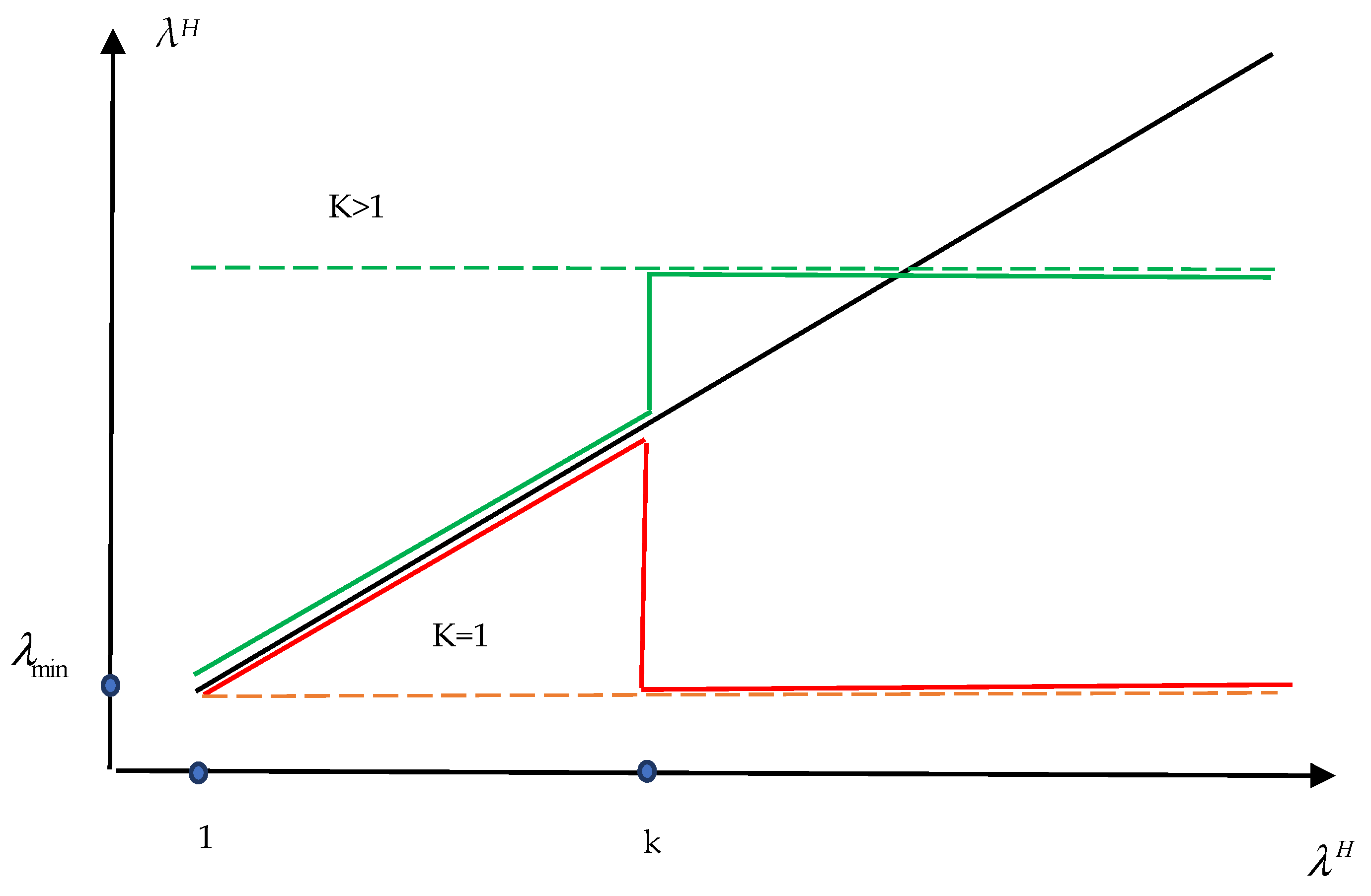
Let us qualitatively investigate the operation of the quasi-Newton BFGS method (71). Taking into account the predominance of eigenvectors with large eigenvalues of the matrix A and, accordingly, small eigenvalues of the matrix A⁻¹ = H, it is possible to qualitatively display the picture of the reconstruction of the matrix A⁻¹ eigenvectors for different values of K, making a rough assumption that small eigenvalues are sequentially restored. A rough diagram of the process of reconstructing the spectrum of matrix eigenvalues is shown in Figure 2.

One of the components of increasing the degree of orthogonality of learning vectors in QNMs is the normalization of the initial metric matrix (124). In Section 8, we will consider the impact of the methods noted in this section on increasing the efficiency of QNMs.

8. Numerical Study of Ways to Increase the Orthogonality of Learning Vectors in Quasi-Newton Methods

We implemented and compared quasi-Newtonian BFGS and DFP methods. A one-dimensional search procedure with cubic interpolation [41] (exact one-dimensional descent) and a one-dimensional minimization procedure [34] (inexact one-dimensional descent) were used. We used both the classical QNM with the iterations of (1)–(4) (denoted as BFGS and DFP) and the QNM including iterations with additional orthogonalization (116)–(119) in the form of a sequence of iterations (120) (denoted as BFGS_V and DFP_V). The experiments were carried out by varying the coefficients of the initial normalization of the matrices of the QNM metric.

Since the use of quasi-Newtonian methods is justified primarily based on functions with a high degree of conditionality where conjugate gradient methods do not work efficiently, the test functions were selected based on this principle. Since the QNM is based on a quadratic model of a function, its local convergence rate in a certain neighborhood of the current minimum is largely determined by the efficiency of minimizing the ill-conditioned quadratic functions. The test functions are as follows:

(1) $f_1\left(x\right)={\sum }_{i=1}^n{x}_i^2{i}^6,x_0=(10/\mathrm{1,10}/2,\dots ,10/n).$

The optimal value and minimum point are $f_1^{*}=0and{x}^{*}=\left(\mathrm{0,0},\dots ,0\right).$ The condition number of the matrix of second derivatives for some n is $cond\left({\nabla }^2{f}_1\left(x\right)\right)={\lambda }_{max}/{\lambda }_{min}=n^6$. When n = 1000, the condition number will be $cond\left({\nabla }^2{f}_1\left(x\right)\right)={1000}^6={10}^{18}$.

(2) $f_2\left(x\right)={\sum }_{i=1}^n{x}_i^2{\left(\frac{n}{i}\right)}^6,x_0=(\mathrm{10,10},\dots ,10).$

The optimal value and minimum point are $f_2^{*}=0and{x}^{*}=\left(\mathrm{0,0},\dots ,0\right).$ The condition number of the matrix of second derivatives for some n is $cond\left({\nabla }^2{f}_2\left(x\right)\right)={\lambda }_{max}/{\lambda }_{min}=n^6$. When n = 1000, the condition number will be $cond\left({\nabla }^2{f}_2\left(x\right)\right)={1000}^6={10}^{18}$.

(3) $f_3\left(x\right)={\left({\sum }_{i=1}^n{x}_i^{2}i\right)}^r,x_0=\left(\mathrm{1,1},\dots ,1\right),r=2$.

The optimal value and minimum point are $f_3^{*}=0and{x}^{*}=\left(\mathrm{0,0},\dots ,0\right).$ The function f₃ is based on a quadratic function with the condition number of the matrix of second derivatives for some n $cond\left({\nabla }^2{f}_3\left(x\right)\right)={\lambda }_{max}/{\lambda }_{min}=n$. When n = 1000, the condition number will be $cond\left({\nabla }^2{f}_3\left(x\right)\right)=1000$. The topology of the level surfaces of the function f₃ is identical to the topology of the level surfaces of the basic quadratic function. The matrix of second derivatives of a function tends to zero as it approaches the minimum. Consequently, the inverse matrix tends to infinity. The approximation pattern for the matrix of second derivatives in the QNM will correspond to K = 1 in Figure 2. This case makes it difficult to enter a new subspace due to the significant predominance of eigenvalues in the metric matrix in the already surveyed part of the subspace compared to the eigenvalues of the metric matrix in the unsurveyed area.

(4) $f_4\left(x\right)={\sum }_{i=1}^{n/2}[{10}^8·{\left(x_{2i-1}^2-x_{2i}\right)}^2+{(x_{2i-1}-1)}^2],x_0=\left(\mathrm{1.2,1},-\mathrm{1.2,1},\dots ,-\mathrm{1.2,1}\right)$.

The optimal value and minimum point of rescaled multidimensional Rosenbrock function [42] are $f_4^{*}=0and{x}^{*}=\left(\mathrm{1,1},\dots ,1\right).$ This function has a curved ravine with small values of the second derivative in the direction of the bottom of the ravine and large values of the second derivative in the direction of the normal to the bottom of the ravine. The ratio of second derivatives along such directions is approximately 10⁸.

The stopping criterion is

$$f\left(x_{}^k\right)-f^{*}\le \epsilon =10^{-10}.$$

The results of minimizing the presented functions are given in

Table 1. Results of minimization with normalization of matrix (124) at K = 1 and n = 1000.

	Exact Descent				Inexact Descent
	BFGS	BFGS_V	DFP	DFP_V	BFGS	BFGS_V	DFP	DFP_V
f1(x)	1157	1157	1228	1211	1854	1648	-	1762
	2526	2523	2712	2667	3980	3413		3750
f2(x)	2400	2370	-	-	4351	3218	-	-
	5663	5560			9908	7242
f3(x)	1404	1396	-	1643	1905	1508	5837	2497
	3206	3190		3743	4286	3394	13,362	5686
f4(x)	3328	2964	-	-	-	-	-	-
	7455	6668

and

Table 2. Results of minimization with normalization of matrix (124) at K = 10,000 and n = 1000. For results marked with an asterisk, K = 100.

	Exact Descent				Inexact Descent
	BFGS	BFGS_V	DFP	DFP_V	BFGS	BFGS_V	DFP	DFP_V
f1(x)	1038	1038	1041	1041	1221	1189	1307	1260
	2194	2193	2197	2195	2190	2116	2431	2343
f2(x)	791	795	1091	852	1386	1012	2524	1509
	1863	1874	2560	2028	3129	2159	5794	3341
f3(x)	1082 *	1090 *	8977 *	1343 *	1281	1129	4281	1845
	2436	2454	20,201	3055	2802	2453	9742	4183
f4(x)	4062 *	3850*	-	-	-	-	-	-
	9135	8686

for n = 1000. The problem was considered solved if the method, within the allotted number of iterations and calculations of the function and gradient, reached a function value that satisfied the stopping criterion. The cell indicates the number of iterations (one-dimensional searches along a direction), and below is the number of calls to the function procedure, where the function and gradient are calculated simultaneously. The number of iterations in all tests were limited to 40,000. If the costs of the method exceeded the specified number of iterations, the method was stopped. It was believed that no solution had been found by this method. The dash sign indicates options where a solution could not be obtained. In cases where there was no solution, looping of methods occurred due to the smallness of the minimization steps and, as a consequence, large errors in the gradient differences used in the transformation operations of metric matrices.

Let us consider the effects of reducing the convergence rate of the method. For example, for the function f₃, the matrix of second derivatives tends to zero as it approaches the minimum. Consequently, the inverse matrix tends to infinity. The approximation pattern for the matrix of second derivatives in the QNM will correspond to K = 1 in Figure 2. In the explored part of the subspace, the matrix of the QNM grows. Therefore, the slight presence of residuals in this part of the subspace is greatly amplified. In the unexplored part of the space, the eigenvalues are fixed. This case makes it difficult to enter a new subspace due to the significant predominance of eigenvalues in the metric matrix in the explored part of the subspace compared to the eigenvalues of the metric matrix in the unexplored area. In order to enter the unexplored part of the subspace, it is necessary to eliminate the discrepancy in the explored part of the space. As a consequence, when minimizing functions with a high degree of conditionality, the search steps become smaller, the errors in the gradient differences increase, and the minimization method becomes loopy.

For exact descent, there are practically no differences between the BFGS and BFGS_V methods. In exact descent, successive descent vectors for quadratic functions are conjugated, and matrix learning, considered in a coordinate system with an identity matrix of second derivatives, is carried out using an orthogonal system of vectors. Minor errors lead to the fact that this orthogonality is violated, which affects the DFP method.

For inexact descent, the BFGS_V method significantly outperforms the BFGS method. The DFP and DFP_V methods are practically ineffective on these tests, although the DFP_V method shows better results.

Thus, with one-dimensional search errors, the BFGS_V algorithm is significantly more effective than the BFGS method. The DFP method is practically not applicable when the problem is highly conditioned.

Table 2 shows the experimental data with normalization of the matrix (124) at K > 1. For the functions f₃(x) and f₄(x), the coefficient K had to be reduced to obtain a more effective result.

The initial normalization of the metric matrices, as follows from the results of Table 1 and Table 2, significantly improves the convergence of QNMs. The situation corresponds to the case in Figure 2 for K > 1. Large eigenvalues in the unexplored part of the subspace make it easy to find new conjugate directions and efficiently train metric matrices with almost orthogonal training vectors.

For exact descent, there are practically no differences between the BFGS and BFGS_V methods. For inexact descent, the BFGS_V method significantly outperforms the BFGS method. The DFP and DFP_V methods are efficient for functions f₁(x) − f₃(x), while for inexact descent, the DFP_V method significantly outperforms the DFP method.

Thus, in the case of one-dimensional search errors, the BFGS_V algorithm is significantly more efficient than the BFGS method and correct initial normalization of metric matrices can significantly increase the convergence rate of the method.

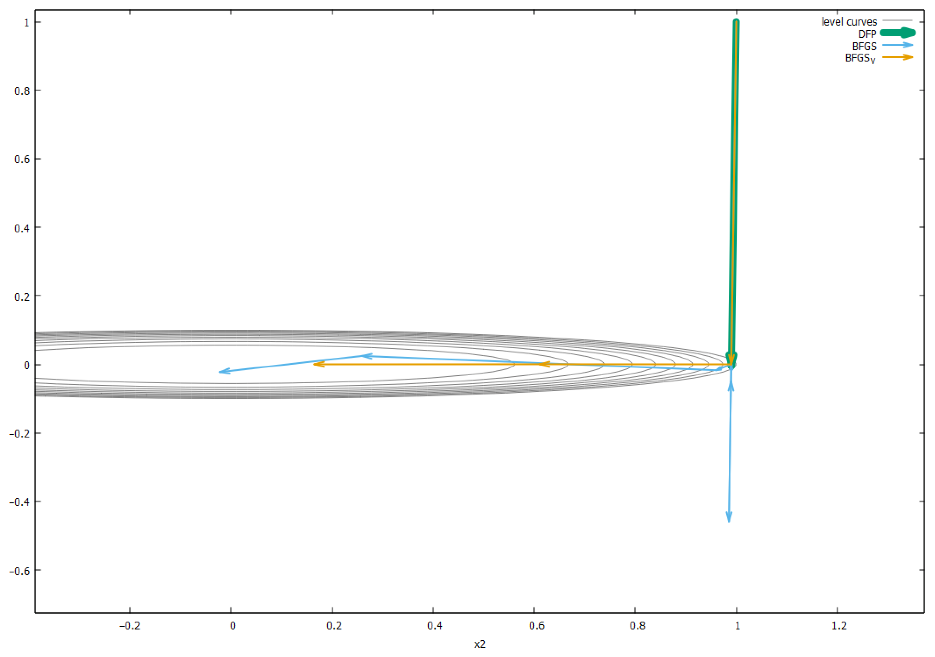
For the purpose of giving a visual demonstration of the method, we minimize a two-dimensional function as follows:

$$f_5\left(x\right)={\left(x_1^2+100x_2^2\right)}^2,x_0=\left(\mathrm{1,1}\right).$$

To test the idea of the efficiency of orthogonalization to increase the performance of the quasi-Newton method, to adversely affect the minimization conditions, the initial matrix was normalized at K = 0.000001, which should significantly complicate the solution of the problem and reveal the effect of the advantages of the degree of orthogonality of the learning vectors of the BFGS and BFGS_V methods over the DFP method.

The stopping criterion was

$$f\left(x_{}^k\right)-f^{*}\le \epsilon =10^{-2}$$

The results are shown in

Table 3. Results of minimization with normalization of matrix (124) at K = 0.000001 and n = 2.

	Exact Descent
	BFGS	BFGS_V	DFP_V
Number of iterations	13	5	3733
Fmin	2.5862 × 10−3	7.5003 × 10−4	7.7552 × 10−3

. The row with f₅(x) shows the number of iterations, while the row with f_min shows the minimal function value achieved.

The path of three considered algorithms is shown in Figure 3.

Here, theoretical results of the influence of the orthogonality degree of matrix learning vectors on the convergence rate of the method are confirmed. The BFGS_V method performs forced orthogonalization, which improves the result of the BFGS method. The trajectories of the methods are listed in

Table A1. Trajectory of the BFGS_V method moving.

Iteration	f5(x)	x1	x2
0	0.0	1.0	1.0
1	9.605985 × 10−1	9.900005 × 10−1	5.073008 × 10−5
2	9.605986 × 10−1	9.900005 × 10−1	5.332304 × 10−5
3	9.605988 × 10−1	9.900006 × 10−1	5.659179 × 10−5
4	1.396454 × 10−1	6.112994 × 10−1	2.122674 × 10−4
5	7.500359 × 10−4	1.654885 × 10−1	5.745936 × 10−5

,

Table A2. Trajectory of the BFGS method moving.

Iteration	f5(x)	x1	x2
0	0.0	1.0	1.0
1	4.865982 × 102	9.854078 × 10−1	−4.592161 × 10−1
2	1.489919	9.895086 × 10−1	−4.914216 × 10−2
3	9.608406 × 10−1	9.899878 × 10−1	−1.220497 × 10−3
4	9.605957 × 10−1	9.899999 × 10−1	−6.968405 × 10−6
5	9.605941 × 10−1	9.899990 × 10−1	−1.031223 × 10−4
6	9.605941 × 10−1	9.899990 × 10−1	−9.891454 × 10−5
7	9.605941 × 10−1	9.899990 × 10−1	−9.945802 × 10−5
8	9.612290 × 10−1	9.899966 × 10−1	1.815384 × 10−3
9	9.641387 × 10−1	9.899999 × 10−1	−4.249478 × 10−3
10	9.605818 × 10−1	9.899963 × 10−1	9.036299 × 10−6
11	9.059276 × 10−1	9.603298 × 10−1	−1.719565 × 10−2
12	1.634266 × 10−2	2.596599 × 10−1	2.457950 × 10−2
13	2.586155 × 10−3	−2.187391 × 10−2	−2.244455 × 10−2

and

Table A3. Trajectory of the DFP method moving.

Iteration	f5(x)	x1	x2
0	0.0	1.0	1.0
1	9.605985 × 10−1	9.900005 × 10−1	5.073008 × 10−5
2	9.605986 × 10−1	9.900005 × 10−1	5.332304 × 10−5
3	9.605988 × 10−1	9.900006 × 10−1	5.659179 × 10−5
4	9.605991 × 10−1	9.900006 × 10−1	6.073300 × 10−5
5	9.605994 × 10−1	9.900007 × 10−1	6.601199 × 10−5
6	9.605942 × 10−1	9.899988 × 10−1	−1.191852 × 10−4
7	9.605942 × 10−1	9.899988 × 10−1	−1.202172 × 10−4
8	9.605942 × 10−1	9.899988 × 10−1	−1.215724 × 10−4
9	9.605942 × 10−1	9.899988 × 10−1	−1.233791 × 10−4
10	9.605942 × 10−1	9.899987 × 10−1	−1.258332 × 10−4
11	9.605957 × 10−1	9.899999 × 10−1	−8.005638 × 10−6
12	9.605974 × 10−1	9.899977 × 10−1	−2.294417 × 10−4
13	9.605962 × 10−1	9.900000 × 10−1	4.809401 × 10−6
14	9.605946 × 10−1	9.899985 × 10−1	−1.494894 × 10−4
15	9.605941 × 10−1	9.899992 × 10−1	−8.356599 × 10−5
16	9.605941 × 10−1	9.899990 × 10−1	−1.019703 × 10−4
17	9.605941 × 10−1	9.899990 × 10−1	−9.866443 × 10−5
18	9.605941 × 10−1	9.899990 × 10−1	−9.826577 × 10−5
19	9.605941 × 10−1	9.899990 × 10−1	−9.914318 × 10−5
20	9.605941 × 10−1	9.899990 × 10−1	−9.806531 × 10−5
21	9.639558 × 10−1	9.899569 × 10−1	−4.240006 × 10−3
22	9.605941 × 10−1	9.899991 × 10−1	−9.292366 × 10−5
23	9.605942 × 10−1	9.899988 × 10−1	−1.237791 × 10−4
24	9.605943 × 10−1	9.899994 × 10−1	−6.417724 × 10−5
25	9.605943 × 10−1	9.899986 × 10−1	−1.365365 × 10−4
26	9.605942 × 10−1	9.899992 × 10−1	−7.609652 × 10−5
27	9.605941 × 10−1	9.899989 × 10−1	−1.126456 × 10−4
28	9.605941 × 10−1	9.899990 × 10−1	−9.613542 × 10−5
29	9.605941 × 10−1	9.899990 × 10−1	−1.018252 × 10−4
30	9.605941 × 10−1	9.899990 × 10−1	−1.002864 × 10−4
31	9.605941 × 10−1	9.899990 × 10−1	−1.007205 × 10−4
32	9.605941 × 10−1	9.899990 × 10−1	−1.001624 × 10−4
33	9.605941 × 10−1	9.899990 × 10−1	−1.006906 × 10−4
34	9.605941 × 10−1	9.899990 × 10−1	−1.000533 × 10−4
35	9.605941 × 10−1	9.899990 × 10−1	−1.006925 × 10−4
36	9.605941 × 10−1	9.899990 × 10−1	−9.993761 × 10−5
37	9.605941 × 10−1	9.899990 × 10−1	−1.007145 × 10−4
38	9.605941 × 10−1	9.899990 × 10−1	−9.980530 × 10−5
39	9.605941 × 10−1	9.899990 × 10−1	−1.007537 × 10−4
40	9.605941 × 10−1	9.899990 × 10−1	−9.964890 × 10−5
41	9.605941 × 10−1	9.899990 × 10−1	−1.008103 × 10−4

of Appendix A (the trajectory of the DFP method is shown partially).

9. Conclusions

This paper presents methods for converting metric matrices in quasi-Newton methods based on gradient learning algorithms. As a result, it is possible to represent the system of learning steps in the form of an algorithm for minimizing a certain objective function along a system of directions and to draw conclusions about the convergence rate of the learning process based on the properties of this system of directions. The main conclusion is that the convergence rate is directly dependent on the degree of orthogonality of the learning vectors.

Based on the study of learning algorithms in the DFP and BFGS methods, it is possible to show that the degree of orthogonality of the learning vectors in the BFGS method is higher than that in the DFP method. This means that entering the unexplored region of the minimization space due to the noise and inaccuracies of one-dimensional descent in the DFP method is more difficult than in the BFGS method, which explains why the BFGS updating formula has the best results.

As a result of studies on quadratic functions, it has been revealed that the dimension of the minimization space is reduced when iterations with an exact one-dimensional descent or iterations with additional orthogonalization are included in the quasi-Newton method. It is shown that it is also possible to increase the orthogonality of the learning vectors and thereby increase the convergence rate of the method through special normalization of the initial metric matrix. The theoretically predicted effects of increasing the efficiency of quasi-Newton methods were confirmed as a result of a computational experiment on complex ill-conditioned minimization problems. In future work, we plan to study minimization methods under the conditions of a linear background that adversely affects the convergence.