Article

Study of the Six-Compartment Nonlinear COVID-19 Model with the Homotopy Perturbation Method

1
Department of Mathematics, COMSATS University Islamabad, Lahore Campus, Lahore 54000, Pakistan
2
Department of Electronics Engineering, Sir Syed University of Engineering & Technology, Karachi 75300, Pakistan
3
National Laboratory for Health Security, Bolyai Institute, University of Szeged, Aradi Vértanúk Tere 1, 6720 Szeged, Hungary
4
Department of Mathematics, Faculty of Science, Mansoura University, Mansoura 35516, Egypt
*
Author to whom correspondence should be addressed.
Axioms 2024, 13(5), 311; https://doi.org/10.3390/axioms13050311
Submission received: 20 March 2024 / Revised: 1 May 2024 / Accepted: 5 May 2024 / Published: 9 May 2024
(This article belongs to the Special Issue Dynamical Systems: Theory and Applications in Mathematical Biology)

Abstract

:
The current study aims to utilize the homotopy perturbation method (HPM) to solve nonlinear dynamical models, with a particular focus on models related to predicting and controlling pandemics, such as the SIR model. Specifically, we apply this method to solve a six-compartment model for the novel coronavirus (COVID-19), which includes susceptible, exposed, asymptomatic infected, symptomatic infected, and recovered individuals, and the concentration of COVID-19 in the environment is indicated by S ( t ) , E ( t ) , A ( t ) , I ( t ) , R ( t ) , and B ( t ) , respectively. We present the series solution of this model by varying the controlling parameters and representing them graphically. Additionally, we verify the accuracy of the series solution (up to the ( n 1 ) t h -degree polynomial) that satisfies both the initial conditions and the model, with all coefficients correct at 18 decimal places. Furthermore, we have compared our results with the Runge–Kutta fourth-order method. Based on our findings, we conclude that the homotopy perturbation method is a promising approach to solve nonlinear dynamical models, particularly those associated with pandemics. This method provides valuable insight into how the control of various parameters can affect the model. We suggest that future studies can expand on our work by exploring additional models and assessing the applicability of other analytical methods.

1. Introduction

The COVID-19 pandemic has had a significant impact on global health, economies, and societies. It is caused by the SARS-CoV-2 virus, which spreads through respiratory droplets and contact with contaminated surfaces. There are four subtypes of coronavirus, seven of which are known to affect humans. COVID-19 has exacerbated socioeconomic inequalities, particularly along the lines of gender, race, ethnicity, nativity, and class. It has affected employment, income, social welfare spending, and the criminal justice system. The pandemic has also had a profound impact on mental health, with higher levels of anxiety, depression, and stress. However, individuals differ in their ability to cope with the pandemic and some show resilience. Research has been conducted in various fields, including health, mass media, sociology, business, economics, tourism, education, and law, to understand and address the challenges posed by COVID-19.
The role of the environment in the transmission and spread of COVID-19 is a significant aspect to consider in mathematical modeling studies. Environmental contamination by infected individuals and the subsequent impact on the transmission dynamics of the disease have been explored in several articles.
Sarkar et al. [1] proposed a nonlinear mathematical model for COVID-19 transmission in India, which incorporates environmental contamination as a factor. Hussain et al., developed a stochastic mathematical model to analyze the spread and extinction of the disease, considering environmental white noise [2]. Azoz et al., investigated the dynamics of COVID-19 using a model that highlights the importance of the environment as a reservoir for the propagation of disease [3]. There are thousands of COVID-19 models; we refer to some of the latest published review papers on COVID-19 models for further study [4,5,6,7,8,9,10,11].
In [12], a novel mathematical model was developed to analyze the transmission dynamics of COVID-19, taking into account the concentration of the coronavirus in the environment. These studies emphasize the need to understand the environmental mechanisms that contribute to the pandemic and the importance of disinfection measures to control the spread of the virus.
To investigate the dynamics of COVID-19, we employed the COVID-19 model presented in [12], which comprises six compartments: susceptible individuals denoted by S ( t ) , exposed individuals denoted by E ( t ) , asymptomatic infected individuals denoted by A ( t ) , symptomatic infected individuals denoted by I ( t ) , recovered individuals denoted by R ( t ) , and the concentration of COVID-19 in the environment denoted by B ( t ) . The total human population is divided into five different classes, given by M ( t ) = S ( t ) + E ( t ) + A ( t ) + I ( t ) + R ( t ) . The following model equations are given:
d S d t = Λ ( β 1 E + β 2 I + β 3 A + β 4 B ) S M d S , d E d t = ( β 1 E + β 2 I + β 3 A + β 4 B ) S M δ + d E , d I d t = 1 τ δ E ( d + d 1 + γ 1 ) I , d A d t = τ δ E ( d + γ 2 ) A , d R d t = γ 1 I + γ 2 A d R , d B d t = ψ 1 E + ψ 2 I + ψ 3 A ϕ B .
where S ( 0 ) = S 0 0 , E ( 0 ) = E 0 0 , I ( 0 ) = I 0 0 , A ( 0 ) = A 0 0 , R ( 0 ) = R 0 0 , B ( 0 ) = B 0 0 , and ± lim n M ( t ) Λ d . The model parameters are listed in Table 1. The detailed formulations of the model with brief discussion, stability of the model, analysis of equilibrium points, parameter estimations, and sensitivity analysis are given in the research article [12].
Ji Huan He proposed the homotopy perturbation method (HPM) in 1999 [13]; he improved this method and applied it to asymptotology in 2004 [14], nonlinear oscillators with discontinuities [15], limit cycle and bifurcation of nonlinear problems [16], nonlinear wave equations [17], and the boundary value problem [18].
Recently, many scientists and researchers have applied HPM to solve numerous problems which arise in science, technology, and health, such as nonlinear problems arising in heat transfer [19], the nonlinear Burgers’ equation [20], the fractional KdV–Burgers’ equation [21], the Helmholtz–Fangzhu oscillator [22], linear parabolic equations [23], the Balitsky–Kovchegov equation [24], a one-dimensional convection diffusion problem [25], a fractional wave equation [26], a shock wave equation [27], linear fuzzy delay differential equations [28], a mathematical model of dengue fever [29], a mathematical model of the eardrum [30], a mathematical model of mumps [31], systems of second-order nonlinear ordinary differential equations [32], iterative methods for nonlinear equations [33], and a model of depletion of forest resources [34]. Agarwal et al. [35] applied the HPM and Bernoulli equation to measure the COVID-19 outbreak. They concluded that the fractional order performs better than the integer order. Nasution et al. [36] also studied an SEIR model for the spread of COVID-19 using the HPM and RK–fourth-order methods. They focused on the impact of moving the recovered sub-population back to the susceptible sub-population.
In this study, the homotopy perturbation method (HPM) is utilized to solve the COVID-19 model (1), providing a series solution that closely approximates the exact solution. The validity of HPM is established in Section 2, focusing on the convergence of HPM. The series solution for this model is further validated in Section 3.1. It is demonstrated that the series solution outperforms the numerical solution obtained through the RK–fourth-order method, as discussed in Section 3.2. The pertinent parameters crucial for controlling this pandemic disease are thoroughly examined in Section 4, titled Numerical Simulation and Discussion.

2. Homotopy Perturbation Method

To illustrate the homotopy perturbation method [13], we consider a differential equation
D ( μ ) g ( τ ) = 0 , τ ,
subject to the boundary condition
β ( μ , μ τ ) = 0 , τ Γ ,
where D is a differential operator, β is boundary operator, Γ is the boundary of the domain ℧, and g ( τ ) is a known analytic function. The D, generally consist of two parts, a linear and nonlinear part, represented as L and N, respectively. Therefore, (2) can be written as follows:
L ( μ ) + N ( μ ) g ( τ ) = 0 .
Using the homotopy method, by taking an embedding parameter q, one can construct a homotopy w ( τ , q ) : × [ 0 , 1 ] R for Equation (4), which satisfies
H ( w , q ) = ( 1 q ) L ( w ) L ( μ 0 ) + q L ( w ) + N ( w ) g ( τ ) = 0 ,
it is equivalent to
H ( w , q ) = L ( w ) L ( μ 0 ) + q L ( μ 0 ) + q N ( w ) g ( τ ) = 0 ,
where q [ 0 , 1 ] is an embedding parameter and μ 0 is an initial guess approximation of (6), which satisfies the initial (or boundary) conditions. It can be written as follows:
q = 0 , H ( w , 0 ) = L ( w ) L ( μ 0 ) ,
q = 1 , H ( w , 1 ) = L ( w ) + N ( w ) g ( τ ) .
We suppose that the solution is in the form of power series for Equation (5) by taking an embedding parameter q :
w = w 0 + q w 1 + q 2 w 2 + q 3 w 3 + .
The approximate solution of Equation (2) can be obtained by setting q = 1 ,
μ = lim q 1 w = w 0 + w 1 + w 2 + w 3 + .
The convergence of (10) has been proved in [13], which depends upon the nonlinear operator A ( w ) and the following conditions:
  • The second derivative of N ( w ) with respect to w must be small, because the parameter q may be relatively large, i.e., q 1 .
  • The norm of L 1 N / w must be smaller than one, in order for the series to converge.

Convergence of HPM

The convergence of HPM is derived in [37,38] as well. If we consider Equation (6), we can write
L ( w ) L ( v 0 ) = q g ( t ) L ( v 0 ) N ( w ) ,
by using Equation (9) in Equation (11), we get
L i = 0 w i q i L ( v 0 ) = q g ( t ) L ( v 0 ) N i = 0 w i q i ,
when we put q = 1 in L.H.S of Equation (12),
i = 0 L ( w i ) L ( v 0 ) = q g ( t ) L ( v 0 ) N i = 0 w i q i .
According to the Maclaurin expansion of N ( i = 0 w i q i ) with respect to q,
N i = 0 w i q i = n = 0 1 n ! δ n δ q n N i = 0 w i q i q n .
Here,
N i = 0 w i q i N i = 0 n w i q i .
By using Equation (15) in R.H.S of Equation (14),
N i = 0 w i q i = n = 0 1 n ! δ n δ q n N i = 0 n w i q i q n .
Now, we set
H n ( w 0 , w 1 , w 2 , w 3 , ) = 1 n ! δ n δ q n N i = 0 n w i q i q n , n = 1 , 2 , 3 , ,
substituting Equation (17) in Equation (16),
N i = 0 w i q i = n = 0 H n q n .
Using Equation (18) in Equation (13), we have
i = 0 L ( w i ) L ( v 0 ) = q g ( t ) L ( v 0 ) n = 0 H n q n .
By equating the terms with the powers in q,
q 0 : L ( w 0 ) L ( v 0 ) = 0 , q 1 : L ( w 1 ) = g ( t ) L ( v 0 ) H 0 , q 3 : L ( w 3 ) = H 2 , q 4 : L ( w 4 ) = H 3 ,
We derive
w 0 = v 0 , w 1 = L 1 ( g ( t ) ) v 0 L 1 ( H 0 ) , w 2 = L 1 ( H 1 ) , w 3 = L 1 ( H 2 ) , w 4 = L 1 ( H 3 ) ,
We suppose that
S n = w 1 + w 2 + w 3 + w 4 + w 5 + + w n = k = 1 n w k .
Now, we suppose that B is a Banach space, S B .   k = 1 w k converges to s B if ( 0 λ < 1 ) , s.t ( n N | | v n | | λ | | v n 1 | | ).
We need to show that ( S n ) is a Cauchy sequence in the Banach space. For any m , n N , and n m , we derive
| | S n S m | | = | | ( S n S n 1 ) + ( S n 1 S n 2 ) + + ( S m + 1 S m ) | | | | S n S n 1 | | + | | S n 1 S n 2 | | + + | | S m + 1 S m | | λ n | | w 0 | | + λ n 1 | | w 0 | | + + λ m + 1 | | w 0 | | ( λ n + λ n 1 + + λ m + 1 ) | | w 0 | | ( λ m + 1 + + λ n + ) | | w 0 | | λ m + 1 ( 1 + λ + + λ n + ) | | w 0 | | λ m + 1 1 λ | | w 0 | | .
So, lim m , n | | S n S m | | = 0 . Therefore, ( S n ) is a Cauchy sequence in the Banach space and is convergent.

3. Application of HPM

Now, we apply HPM on the model (1) of COVID-19 (nonlinear system of differential equations) as
1 q u S 0 + q u Λ ( β 1 v + β 2 w + β 3 x + β 4 z ) u N d × s = 0 , 1 q v E 0 + q v ( β 1 v + β 2 w + β 3 x + β 4 z ) u N δ + d v = 0 , 1 q w I 0 + q w 1 τ δ v ( d + d 1 + γ 1 ) w = 0 , 1 q x A 0 + q x τ δ v ( d + γ 2 ) x = 0 , 1 q y R 0 + q y γ 1 w + γ 2 x d y = 0 , 1 q z B 0 + q z ψ 1 v + ψ 2 w + ψ 3 x ϕ z = 0 .
The initial guesses for (21) are constant, as defined in [12]:
u 0 ( t ) = S 0 ( t ) = S ( 0 ) = n 1 v 0 ( t ) = E 0 ( t ) = E ( 0 ) = n 2 w 0 ( t ) = I 0 ( t ) = I ( 0 ) = n 3 x 0 ( t ) = A 0 ( t ) = A ( 0 ) = n 4 y 0 ( t ) = R 0 ( t ) = R ( 0 ) = n 5 z 0 ( t ) = B 0 ( t ) = B ( 0 ) = n 6
and we assume the solution of (21):
u = u 0 + q u 1 + q 2 u 2 + q 3 u 3 + , v = v 0 + q v 1 + q 2 v 2 + q 3 v 3 + , w = w 0 + q w 1 + q 2 w 2 + q 3 w 3 + , x = x 0 + q x 1 + q 2 x 2 + q 3 x 3 + , y = y 0 + q y 1 + q 2 y 2 + q 3 y 3 + , z = z 0 + q z 1 + q 2 z 2 + q 3 z 3 + .
Using Equation (23) in Equation (21) and collecting the terms of powers of q, we obtain
q 0 : u 0 = 0 , u 0 ( 0 ) = n 1 , v 0 = 0 , v 0 ( 0 ) = n 2 , w 0 = 0 , w 0 ( 0 ) = n 3 , x 0 = 0 , x 0 ( 0 ) = n 4 , y 0 = 0 , y 0 ( 0 ) = n 5 , z 0 = 0 , z 0 ( 0 ) = n 6 .
q 1 : u 1 = Λ u 0 Λ β 1 v 0 + β 2 w 0 + β 3 x 0 + β 4 z 0 d u 0 d , u 1 ( 0 ) = 0 , v 1 = u 0 Λ β 1 v 0 + β 2 w 0 + β 3 x 0 + β 4 z 0 d δ + d v 0 , v 1 ( 0 ) = 0 , w 1 = δ 1 τ v 0 d + d 1 + γ 1 w 0 , w 1 ( 0 ) = 0 , x 1 = τ δ v 0 ( d + γ 2 ) x 0 , x 1 ( 0 ) = 0 , y 1 = γ 1 w 0 + γ 2 x 0 y 0 d , y 1 ( 0 ) = 0 , z 1 = ψ 1 v 0 + ψ 2 w 0 + ψ 3 x 0 ϕ z 0 , z 1 ( 0 ) = 0 .
q 2 : u 2 = d Λ u 1 ( β 1 v 0 + β 2 w 0 + β 3 x 0 + β 4 z 0 u 0 ) + u 0 ( β 1 v 1 + β 2 w 1 + β 3 x 1 + β 4 z 1 ) u 1 d , u 2 ( 0 ) = 0 , v 2 = d Λ u 1 ( β 1 v 0 + β 2 w 0 + β 3 x 0 + β 4 z 0 ) + u 0 ( β 1 v 1 + β 2 w 1 + β 3 x 1 + β 4 z 1 ) δ + d v 1 , v 2 ( 0 ) = 0 , w 2 = δ 1 τ v 1 d + d 1 + γ 1 w 1 , w 2 ( 0 ) = 0 , x 2 = τ δ v 1 ( d + γ 2 ) x 1 , x 2 ( 0 ) = 0 , y 2 = γ 1 w 1 + γ 2 x 1 y 1 d , y 2 ( 0 ) = 0 , z 2 = ψ 1 v 1 + ψ 2 w 1 + ψ 3 x 1 ϕ z 1 , z 2 ( 0 ) = 0 .
q 3 : u 3 = d Λ u 2 ( β 1 v 0 + β 2 w 0 + β 3 x 0 + β 4 z ) + u 1 ( β 1 v 1 + β 2 w 1 + β 3 x 1 + β 4 z 1 ) + u 0 ( β 1 v 2 + β 2 w 2 + β 3 x 2 + β 4 z 2 ) u 2 d , u 3 ( 0 ) = 0 , v 3 = d Λ u 2 ( β 1 v 0 + β 2 w 0 + β 3 x 0 + β 4 z 0 ) + u 1 ( β 1 v 1 + β 2 w 1 + β 3 x 1 + β 4 z 1 ) + u 0 ( β 1 v 2 + β 2 w 2 + β 3 x 2 + β 4 z 2 ) δ + d v 2 , v 3 ( 0 ) = 0 , w 3 = δ 1 τ v 2 d + d 1 + γ 1 w 2 , w 3 ( 0 ) = 0 , x 3 = τ δ v 2 ( d + γ 2 ) x 2 , x 3 ( 0 ) = 0 , y 3 = γ 1 w 2 + γ 2 x 2 y 2 d , y 3 ( 0 ) = 0 , z 3 = ψ 1 v 2 + ψ 2 w 2 + ψ 3 x 2 ϕ z 2 , z 3 ( 0 ) = 0 .
q 4 : u 4 = d Λ u 0 ( β 1 v 3 + β 2 w 3 + β 3 x 3 + β 4 z 3 ) u 1 ( β 1 v 2 + β 2 w 2 + β 3 x 2 + β 4 z 2 ) u 2 ( β 1 v 1 + β 2 w 1 + β 3 x 1 + β 4 z 1 ) u 3 ( β 1 v 0 + β 2 w 0 + β 3 x 0 + β 4 z 0 ) u 3 d , u 4 ( 0 ) = 0 , v 4 = d Λ u 0 ( β 1 v 3 + β 2 w 3 + β 3 x 3 + β 4 z 3 ) + u 1 ( β 1 v 2 + β 2 w 2 + β 3 x 2 + β 4 z 2 ) + u 2 ( β 1 v 1 + β 2 w 1 + β 3 x 1 + β 4 z 1 ) + u 3 ( β 1 v 0 + β 2 w 0 + β 3 x 0 + β 4 z 0 ) δ + d v 3 , v 4 ( 0 ) = 0 , w 4 = ( δ τ δ ) v 3 ( d + d 1 + γ 1 ) w 3 , w 4 ( 0 ) = 0 , x 4 = δ τ v 3 ( d + γ 2 ) x 3 , x 4 ( 0 ) = 0 , y 4 = ( γ 1 + γ 2 ) x 3 y 3 d , y 4 ( 0 ) = 0 , z 4 = ψ 1 v 3 + ψ 2 w 3 + ψ 3 x 3 ϕ z 3 , z 4 ( 0 ) = 0 .
By integrating Equations (24) to (28) with respect to t considering the initial values, S ( 0 ) = u 0 ( 0 ) = n 1 = 34,813,871 , E ( 0 ) = v 0 ( 0 ) = n 2 = 1 , I ( 0 ) = w 0 ( 0 ) = n 3 = 1 , A ( 0 ) = x 0 ( 0 ) = n 4 = 1 , R ( 0 ) = y 0 ( 0 ) = n 4 = 1 , and B ( 0 ) = z 0 ( 0 ) = n 6 = 1 , and the parameters Λ = 1392.55484 , d = 0.00004 , β 1 = 0.1233 , β 2 = 0.0542 , β 3 = 0.0020 , β 4 = 0.1101 , δ = 0.1980 , τ = 0.3085 , d 1 = 0.0104 , γ 1 = 0.3680 , γ 2 = 0.2945 , ψ 1 = 0.2574 , ψ 2 = 0.2798 , ψ 3 = 0.1584 , and ϕ = 0.3820 [12]; we have the corresponding solution as
u 0 = 34,813,871 , v 0 = 1 , w 0 = 1 , x 0 = 1 , y 0 = 1 , z 0 = 1 .
u 1 = 0.2896 t , v 1 = 0.0915634 t , w 1 = 0.24152 t , x 1 = 0.233454 t , y 1 = 0.662463 t , z 1 = 0.3136 t .
u 2 = 0.0161246 t 2 , v 2 = 0.00706348 t 2 , w 2 = 0.0519682 t 2 , x 2 = 0.0371768 t 2 , y 2 = 0.0788278 t 2 , z 2 = 0.100392 t 2 .
u 3 = 0.00243058 t 3 , v 3 = 0.00289666 t 3 , w 3 = 0.00623319 t 3 , x 3 = 0.00350616 t 3 , y 3 = 0.0100253 t 3 , z 3 = 0.0201991 t 3 .
u 4 = 0.000380499 t 4 , v 4 = 0.000523888 t 4 , w 4 = 0.000490566 t 4 , x 4 = 0.000213939 t 4 , y 4 = 0.000831686 t 4 , z 4 = 0.00269027 t 4 .
By substituting the values of u i , v i , w i , x i , y i , and z i , where 0 i 4 , in Equations (29) to (33) in the assumed solution (23) and taking lim q 1 , we have
S ( t ) = u = 34,813,871 0.2896 t 0.0161246 t 2 + 0.00243058 t 3 0.000380499 t 4 + , E ( t ) = v = 1 + 0.0915634 t + 0.00706348 t 2 0.00289666 t 3 + 0.000523888 t 4 + , I ( t ) = w = 1 0.24152 t + 0.0519682 t 2 0.00623319 t 3 + 0.000490566 t 4 + , A ( t ) = x = 1 0.233454 t + 0.0371768 t 2 0.00350616 t 3 + 0.000213939 t 4 + , R ( t ) = y = 1 + 0.662463 t 0.0788278 t 2 + 0.0100253 t 3 0.000831686 t 4 + , B ( t ) = z = 1 + 0.3136 t 0.100392 t 2 + 0.0201991 t 3 0.00269027 t 4 + .

3.1. Verification of Model and Numerical Results

To verify the validity of the solution, we first verify the solution for initial conditions that are satisfied at t = 0 , then put the solution and its derivatives in the system (model). If both sides of the system are satisfied, we consider the solution to be correct. To verify the second condition, we differentiate the solution given in Equation (34) with respect to t, so we have
d S d t = 0.2896 0.0322493 t + 0.00729174 t 2 0.001522 t 3 + , d E d t = 0.0915634 + 0.014127 t 0.00868997 t 2 + 0.00209555 t 3 + , d I d t = 0.24152 + 0.103936 t 0.0186996 t 2 + 0.00196226 t 3 + , d A d t = 0.233454 + 0.0743536 t 0.0105185 t 2 + 0.000855755 t 3 + , d R d t = 0.662463 0.157656 t + 0.0300758 t 2 0.00332674 t 3 + , d B d t = 0.3136 0.200783 t + 0.0605972 t 2 0.0107611 t 3 + ,
by using Equations (34) and (35), and the parameters Λ = 1392.55484 , d = 0.00004 , β 1 = 0.1233 , β 2 = 0.0542 , β 3 = 0.0020 , β 4 = 0.1101 , δ = 0.1980 , τ = 0.3085 , d 1 = 0.0104 , γ 1 = 0.3680 , γ 2 = 0.2945 , ψ 1 = 0.2574 , ψ 2 = 0.2798 , ψ 3 = 0.1584 , and ϕ = 0.3820 in the system (1), we have
0.000775602 + 1.38778 × 10 17 t 2.60209 × 10 18 t 2 2.1684 × 10 19 t 3 0.0002046 t 4 + = 0 , 1.21431 × 10 18 t 1.73472 × 10 18 t 3 + 1.0842 × 10 18 t 3 + 0.000308335 t 4 + = 0 , 3.46945 × 10 18 t 2 + 1.19262 × 10 18 t 3 + 0.000113919 t 4 + = 0 , 1.387782 × 10 17 t + 1.73472 × 10 18 t 2 + 7.86047 × 10 19 t 3 + 0.0000310121 t 4 + = 0 , 3.46945 × 10 18 t 2 8.67362 × 10 19 t 3 0.000243564 t 4 + = 0 , 0 . 2.77556 × 10 17 t 1.38778 × 10 17 t 2 1.73472 × 10 18 t 3 0.00133203 t 4 + = 0 .
The coefficients of the t powers in (36) are correct at zero or closer to zero (approximately 18 to 19 decimal places). It means that the solution satisfies the model. Our series solution is up to fourth-degree polynomials, which satisfies the system up to the third-degree polynomial (where the coefficients are closer to zero). The solution can be improved by taking/adding more power t terms (or HPM iterations).

3.2. Runge–Kutta Method and Error Analysis

We will now compare the HPM-derived series solution of our model, Equation (1) with a well-known numerical method called the Runge–Kutta fourth-order method. This method is readily available in undergraduate mathematics textbooks. We adapt our model according to this method and obtain results with different step sizes; then, we calculate the absolute error comparing with our obtained series solutions which are shown in Table 2, Table 3 and Table 4. In these tables, we have shown some values of absolute errors, e S , e E , e I , e A , e R , and e B for S ( t ) , E ( t ) , I ( t ) , A ( t ) , R ( t ) , and B ( t ) , respectively. In Table 2, the absolute error is very high at step size h = 0.1 . In Table 3, the step size is kept smaller and the absolute error is slightly reduced at h = 0.001 . In Table 4, the step size is further reduced by h = 0.001 and the absolute error is significantly reduced. It can be seen here that, for the RK method, we have to keep the step size very small, while in our series solution, there is no need to do so. In the verification paragraph above, we have checked the series solution to see how standard it is in this regard. With such a small step size, the RK method becomes computationally expensive.

4. Numerical Simulation and Discussion

In this section, we discuss the numerical results of the COVID-19 model (1). Figure 1 depicts the upward trajectory of E ( t ) , representing the exposed population, and I ( t ) , representing symptomatic infected individuals, both of which exhibit a comparable rate of increase from time 0 to time 250. Furthermore, A ( t ) , denoting the number of asymptomatic infected individuals, experiences an incremental increase, although at a slower pace. The count of individuals who are infected but do not display symptoms is on the rise; however, the rate of increase is comparatively slower than that of the exposed and symptomatic infected individuals. Conversely, the number of individuals in the recovered state, R ( t ) , and those afflicted with COVID-19, B ( t ) , rises over time, displaying a positive trend. The population’s suitability S ( t ) or vulnerability to the virus exhibits a positive decrease over time. This observation implies that, as time progresses, the population’s susceptibility decreases, potentially attributed to immunity or other influencing factors. It is imperative to acknowledge that the aforementioned interpretation is based solely on the descriptions provided.
  • Susceptible with β 1 , β 2 , β 3 , and β 4 :
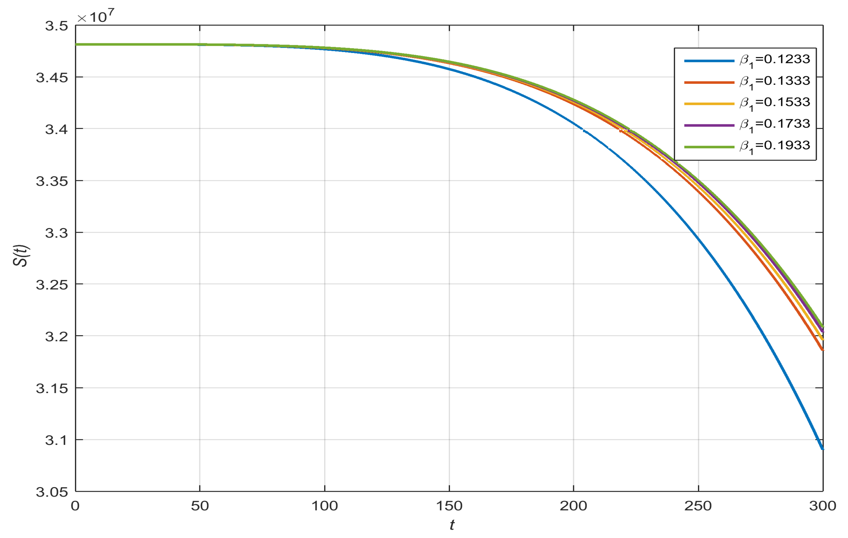
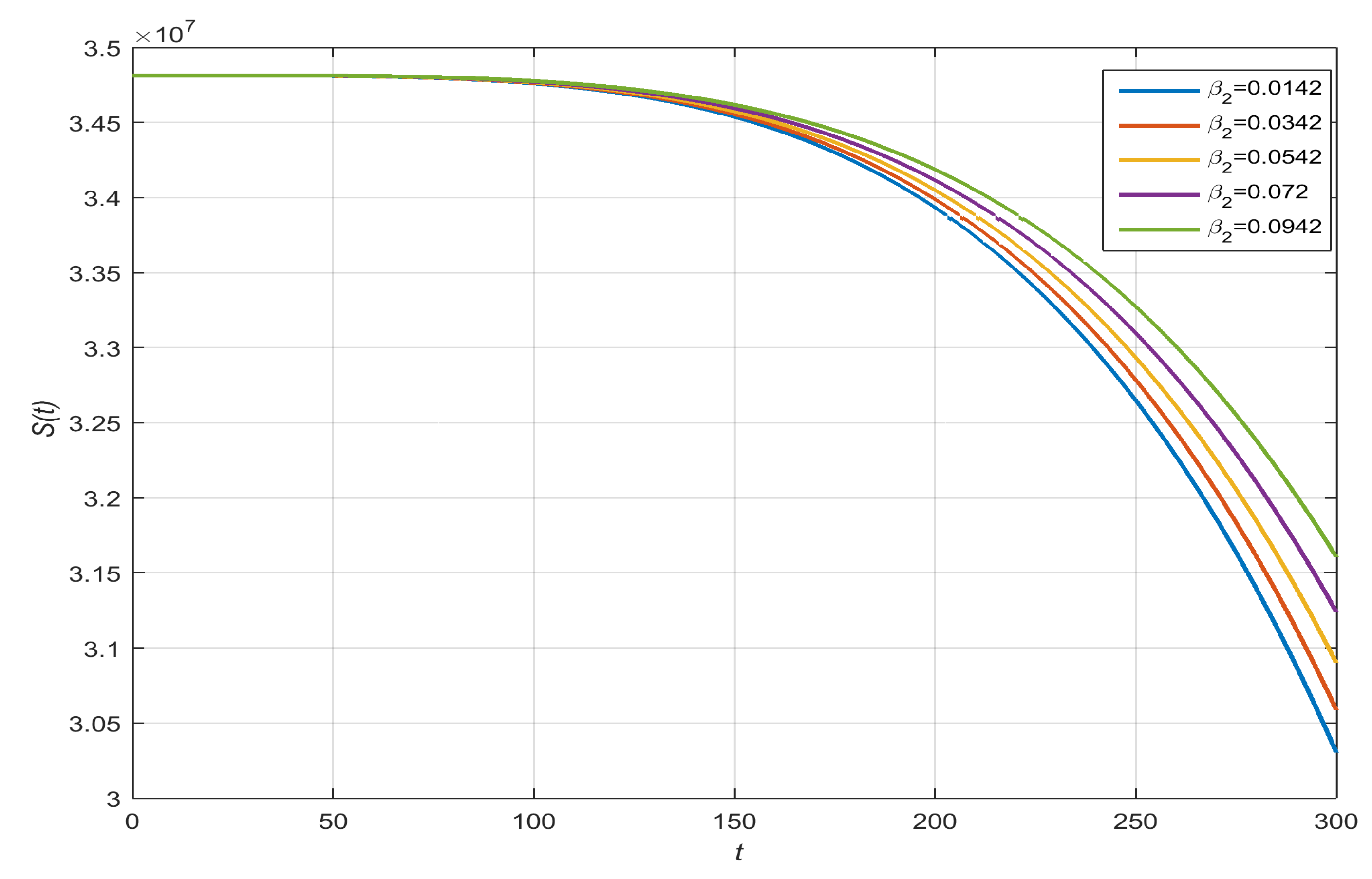
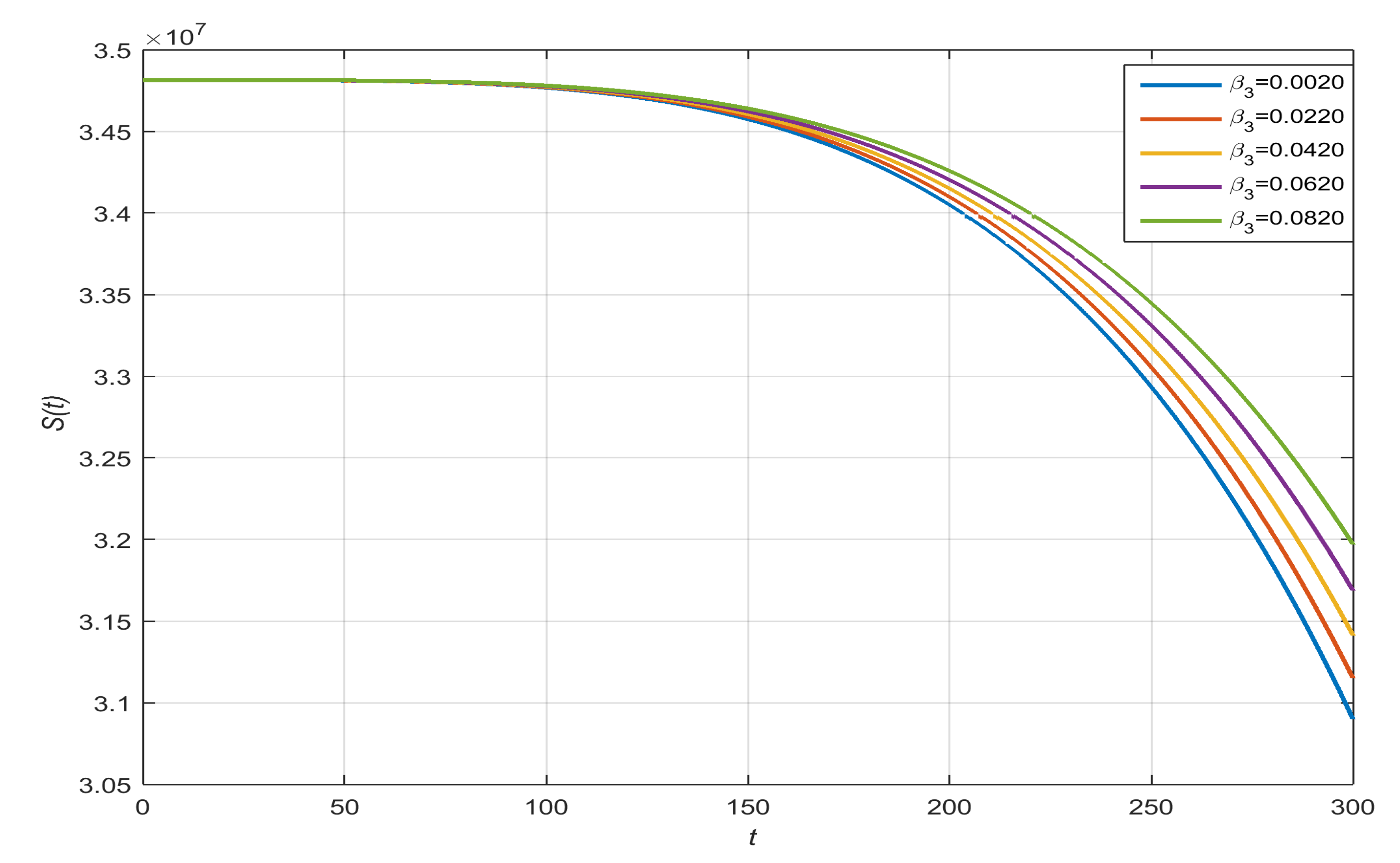
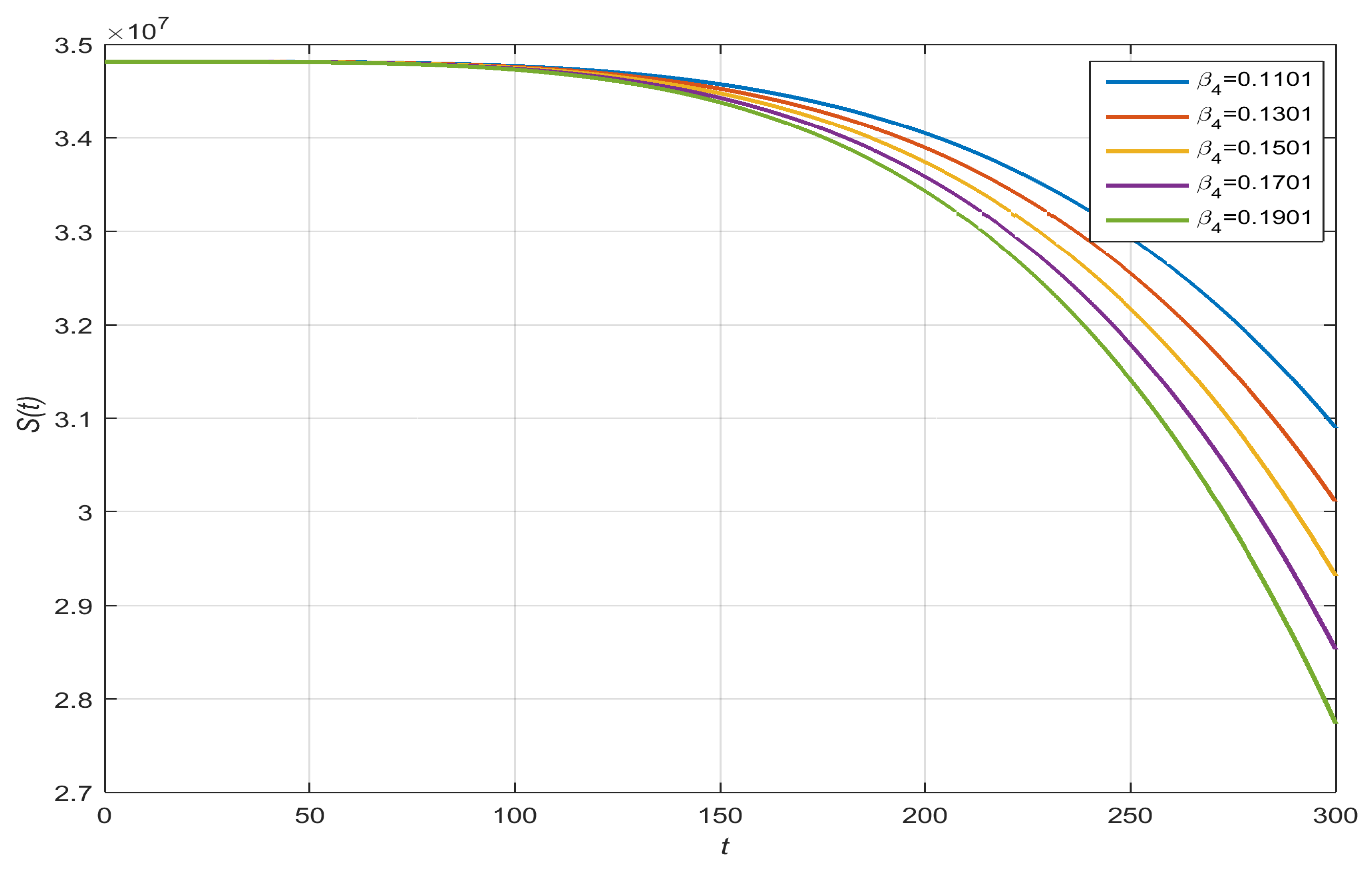
We examined certain parameters of the model as described in the literature, specifically the recruitment rate (birth) and the natural death rate. Subsequently, we conducted an analysis by altering the parameter values. The graphical representation of the impact of these parameters on the susceptible population is depicted in Figure 2, Figure 3, Figure 4 and Figure 5 with respect to the parameters β 1 , β 2 , β 3 , and β 4 .
Figure 2 shows β 1 , the contact rate between exposed and susceptible people. The rate of interaction between those who are vulnerable and those who have been exposed to the virus is influenced by this parameter. As depicted in Figure 2, an increase in β 1 results in a gradual decrease in the susceptibility of individuals. This implies that a reduction in the rate of contact between exposed and susceptible individuals leads to a decrease in the number of cases of susceptibility. In particular, within the framework of Figure 2, it is demonstrated that a decrease in the contact rate ( β 1 ) between susceptible and exposed individuals leads to an increase in the vulnerability of the population. β 3 is a contact rate among asymptomatic infected and susceptible people. Similarly to β 1 , β 3 denotes contact frequency, and it has been noted that variations in β 3 affect susceptibility in a manner comparable to variations in β 1 . If a decrease in β 3 results in a increased susceptibility, this implies that diminishing the contact frequency linked to an alternative facet of the ailment (potentially associated with a distinct demographic or mode of transmission) also renders the populace more susceptible, as seen in Figure 4. β 2 is the contact rate among symptomatic infected and susceptible people and β 4 is a contact rate among the concentration of COVID-19 in the environment and susceptible people. Parameters β 2 and β 4 are observed to exhibit a consistent susceptibility at the highest rate of variables. This indicates that changes in β 2 and β 4 do not seem to affect susceptibility in the same way as changes in β 1 and β 3 do at higher values. The susceptibility retains a constant value at its utmost level, which could indicate that these particular parameters do not have a notable effect on the susceptibility of the population at higher values, as seen in Figure 3 and Figure 5.
  • Exposed People with β 1 , β 2 , β 3 , and β 4 :
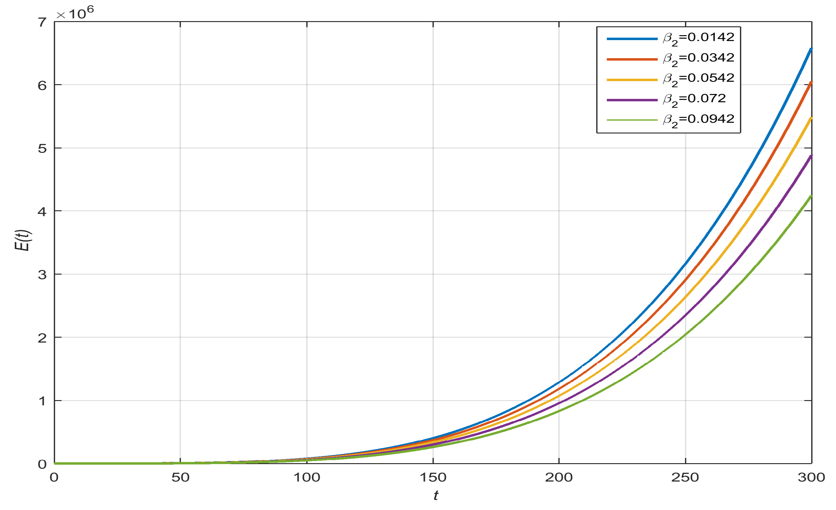
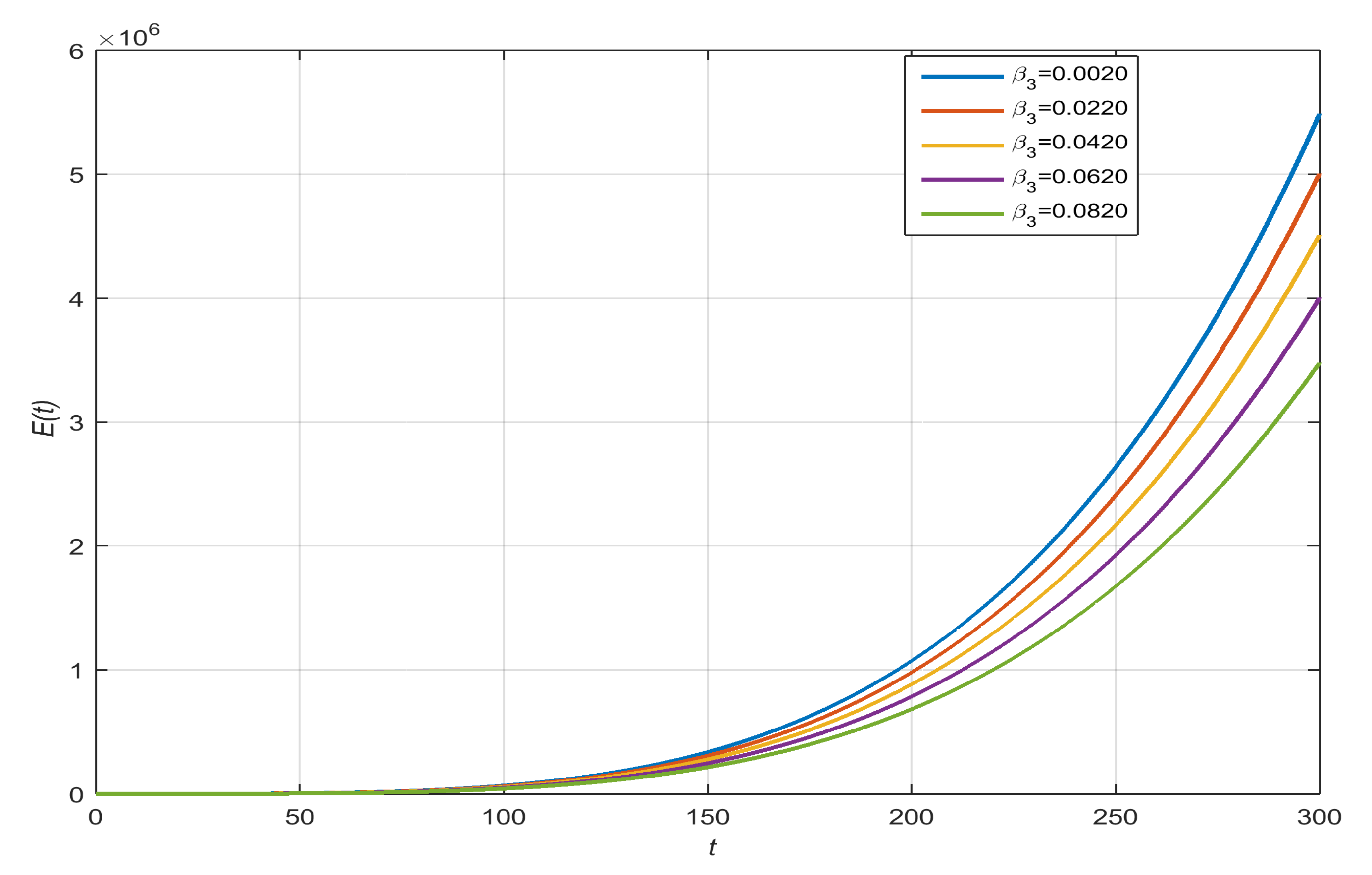
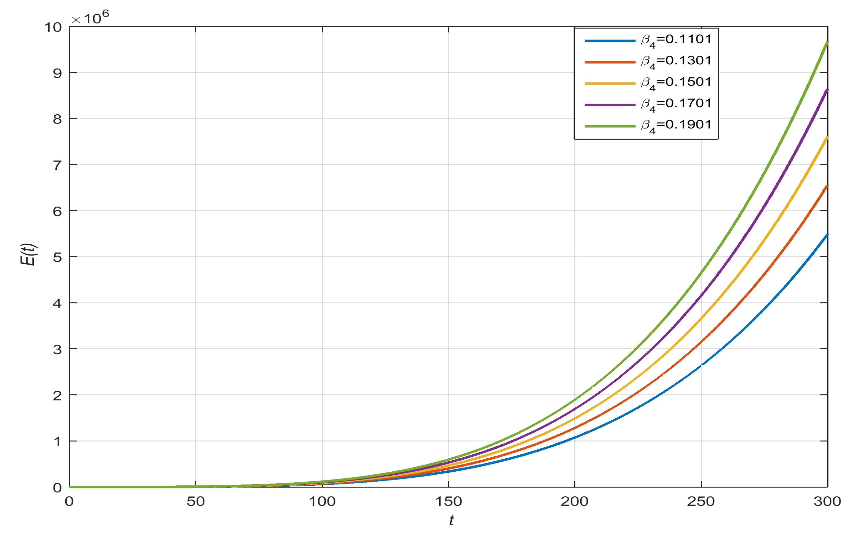
The impact of parameters β 1 , β 2 , β 3 , and β 4 on exposed people is shown graphically in Figure 6, Figure 7, Figure 8 and Figure 9. It can be seen that, by decreasing the values of β 1 , β 2 , β 3 , and β 4 , the exposed cases decrease. Figure 6 shows that the number of exposed persons reduces as β 1 increases. This implies that there is a negative relationship between the population of exposed persons and the contact rate linked to β 1 . That is, there may be a correlation between decreased exposure and increased contact. Figure 7 and Figure 8 provide evidence for a relationship in which the number of exposed people gradually increases at lower β 2 and β 3 values before reaching positive values. This suggests that the population of exposed persons gradually increases at reduced contact rates or transmission rates related to β 2 and β 3 . Figure 9 shows that the number of exposed people decreases further into the negative as the value β 4 drops. This suggests that lowering the rate of β 4 -associated contact or transmission has an adverse effect on the population of exposed persons.
  • Concentration of COVID-19 with ψ 1 , ψ 2 , ψ 3 , and ϕ :
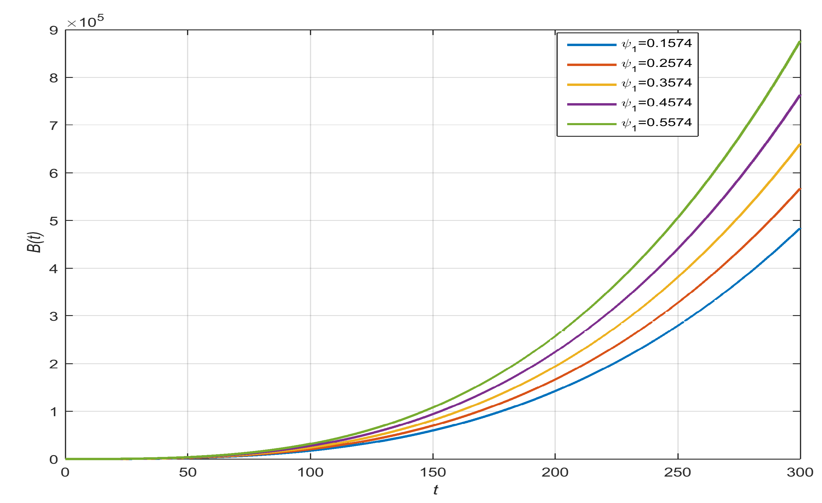
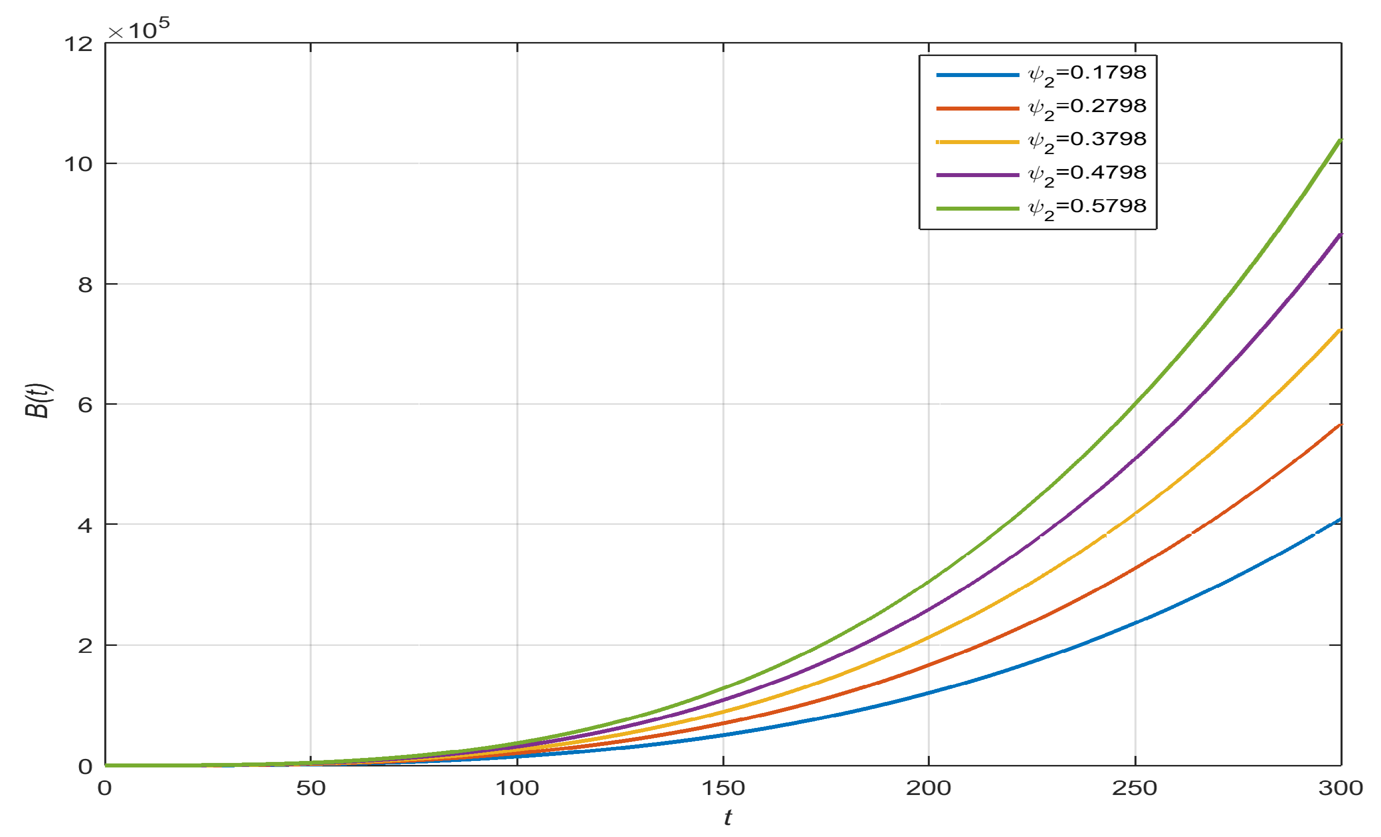
Figure 10, Figure 11, Figure 12 and Figure 13 demonstrate how the concentration of COVID-19 in the environment increases in tandem with increases in ψ 1 , ψ 2 , and ψ 3 levels. This implies that there is a positive relationship between these variables and viral concentration. Practically speaking, this could imply that the elements associated with ψ 1 , ψ 2 , and ψ 3 contribute to an increased level of COVID-19 in the environment.
Figure 13 shows that the concentration of COVID-19 in the environment falls as the parameter ϕ decreases. This suggests that there is a positive relationship between viral concentration and ϕ . Stated differently, a decrease in the amount of COVID-19 present in the environment is associated with an increase in the value of ϕ .
The homotopy perturbation approach, a mathematical strategy for approximating solutions to problems that might not have exact analytical solutions, was applied to solve the COVID-19 model. The resultant solution took the shape of a general series, which most likely reflects a formula that encapsulates the dynamics of the COVID-19 model. To obtain a specific series solution, values were given for the parameters and initial circumstances. This was achieved by putting actual values into the general series solution to obtain a more tangible model representation. After that, the specific series solution was acquired by applying the specified initial circumstances and parameter values. The analysis in this work involved changing the values of the parameters to see how the model was affected. Understanding how various factors affect the dynamics of the COVID-19 model requires this kind of investigation. Plots were created to graphically display the model output. These charts perhaps illustrate how different factors impact different parts of the dynamics of COVID-19. Mathematical modeling frequently involves this kind of effort, particularly when addressing complicated systems such as infectious diseases. It enables researchers to learn more about how the system behaves in various scenarios and with varying parameter values.

5. Conclusions

In this study, we successfully employed the homotopy perturbation method to solve a nonlinear dynamical model of COVID-19. The model consists of six compartments representing susceptible, exposed, asymptomatic infected, symptomatic infected, and recovered individuals, and the concentration of the virus in the environment. We obtained the general solution of the model based on variable conditions and parameters, as well as particular series solutions using initial conditions and specific tested values of parameters. We discussed the convergence of the homotopy perturbation method. The precision of the series solution was verified up to the ( n 1 ) t h -degree polynomial with all coefficients correct at 18 decimal places. Furthermore, we have analyzed the effects of four control parameters ( β 1 , β 2 , β 3 , and β 4 ) on susceptible and exposed populations, as well as the effects of four other control parameters ( ψ 1 , ψ 2 , ψ 3 , and ϕ ) on virus concentration in the environment. With the help of the RK–fourth-order method, we have presented the importance of HPM. Our findings suggest that these parameters should be considered important control parameters for pandemic disease management. Overall, the results of this study demonstrate the effectiveness of the homotopy perturbation method in solving complex nonlinear models and provide useful insights for public health decision-making during pandemics.
While this study successfully applies the homotopy perturbation method (HPM) to a nonlinear COVID-19 model, several critical areas for future research and improvement are evident. The model assumptions should be validated against real-world data to enhance accuracy and realism, potentially requiring adjustments or additional compartments. Comprehensive sensitivity analyses are crucial to identify key parameters that affect disease dynamics, and further calibration of the model against empirical data is needed to improve predictive capabilities. Future studies should extend the model to incorporate spatial and temporal dynamics, considering spatial heterogeneity and behavioral influences, such as compliance with interventions and changes in mobility. Comparative evaluations with other modeling approaches would provide information on the strengths and limitations of HPM in epidemiological modeling. Addressing these aspects will refine the structure of the model, improve the validation processes, and expand the scope of the analysis, ultimately improving the relevance and reliability of such models for pandemic response strategies.

Author Contributions

Methodology, M.R., M.A., D.J. and M.A.I.; software, M.R., M.A., D.J. and M.A.I.; validation, M.R., M.A., D.J. and M.A.I. All authors have read and agreed to the published version of the manuscript.

Funding

M.A.I. was supported by the project No. 146210, implemented with the support provided from the National Research, Development and Innovation Fund of Hungary, financed under the PD_23 funding scheme, by the National Laboratory for Health Security, RRF-2.3.1-21-2022-00006, and by the project No. 129877, implemented with the support provided from the National Research, Development and Innovation Fund of Hungary, financed under the KKP_19 funding scheme.

Institutional Review Board Statement

Not applicable.

Informed Consent Statement

Not applicable.

Data Availability Statement

No new data were created or analyzed in this study. Data sharing is not applicable to this article.

Conflicts of Interest

The authors declare no conflicts of interest.

References

  1. Sarkar, K.; Mondal, J.; Khajanchi, S. How do the contaminated environment influence the transmission dynamics of COVID-19 pandemic? Eur. Phys. J. Spec. Top. 2022, 231, 3697–3716. [Google Scholar] [CrossRef]
  2. Hussain, S.; Madi, E.N.; Khan, H.; Gulzar, H.; Etemad, S.; Rezapour, S.; Kaabar, M.K. On the stochastic modeling of COVID-19 under the environmental white noise. J. Funct. Spaces 2022, 2022, 4320865. [Google Scholar] [CrossRef]
  3. Azoz, S.; Abdelhakiem, K.; Hussien, F. COVID-19 Mathematical Study with Environmental Reservoirs and Three General Functions for Transmissions. Authorea Prepr. 2022, 12, 951–968. [Google Scholar]
  4. Afzal, A.; Saleel, C.A.; Bhattacharyya, S.; Satish, N.; Samuel, O.D.; Badruddin, I.A. Merits and limitations of mathematical modeling and computational simulations in mitigation of COVID-19 pandemic: A comprehensive review. Arch. Comput. Methods Eng. 2022, 29, 1311–1337. [Google Scholar] [CrossRef] [PubMed]
  5. Saleem, F.; Al-Ghamdi, A.S.A.M.; Alassafi, M.O.; AlGhamdi, S.A. Machine learning, deep learning, and mathematical models to analyze forecasting and epidemiology of COVID-19: A systematic literature review. Int. J. Environ. Res. Public Health 2022, 19, 5099. [Google Scholar] [CrossRef] [PubMed]
  6. Rahimi, I.; Chen, F.; Gandomi, A.H. A review on COVID-19 forecasting models. Neural Comput. Appl. 2023, 35, 23671–23681. [Google Scholar] [CrossRef]
  7. Pozo-Martin, F.; Beltran Sanchez, M.A.; Müller, S.A.; Diaconu, V.; Weil, K.; El Bcheraoui, C. Comparative effectiveness of contact tracing interventions in the context of the COVID-19 pandemic: A systematic review. Eur. J. Epidemiol. 2023, 38, 243–266. [Google Scholar] [CrossRef]
  8. Khalilpourazari, S.; Hashemi Doulabi, H. Robust modelling and prediction of the COVID-19 pandemic in Canada. Int. J. Prod. Res. 2023, 61, 8367–8383. [Google Scholar] [CrossRef]
  9. Moreau, J. Systematic Review of Mathematical Models for Viral Transmission Dynamics: Insights from COVID-19 Studies. Lett. Biomath. 2024, 11, 21–30. [Google Scholar]
  10. Naidoo, M.; Shephard, W.; Kambewe, I.; Mtshali, N.; Cope, S.; Rubio, F.A.; Rasella, D. Incorporating social vulnerability in infectious disease mathematical modelling: A scoping review. BMC Med. 2024, 22, 125. [Google Scholar] [CrossRef]
  11. Liu, Y.; Yin, Y.; Ward, M.P.; Li, K.; Chen, Y.; Duan, M.; Zhang, Z. Optimization of Screening Strategies for COVID-19: Scoping Review. JMIR Public Health Surveill. 2024, 10, e44349. [Google Scholar] [CrossRef] [PubMed]
  12. Alqarni, M.S.; Alghamdi, M.; Muhammad, T.; Alshomrani, A.S.; Khan, M.A. Mathematical modeling for novel coronavirus (COVID-19) and control. Numer. Methods Partial. Differ. Equ. 2022, 38, 760–776. [Google Scholar] [CrossRef] [PubMed]
  13. He, J.H. Homotopy perturbation technique. Comput. Methods Appl. Mech. Eng. 1999, 178, 257–262. [Google Scholar] [CrossRef]
  14. He, J.H. Asymptotology by homotopy perturbation method. Appl. Math. Comput. 2004, 156, 591–596. [Google Scholar] [CrossRef]
  15. He, J.H. The homotopy perturbation method for nonlinear oscillators with discontinuities. Appl. Math. Comput. 2004, 151, 287–292. [Google Scholar] [CrossRef]
  16. He, J.H. Limit cycle and bifurcation of nonlinear problems. Chaos Solitons Fractals 2005, 26, 827–833. [Google Scholar] [CrossRef]
  17. He, J.H. Application of homotopy perturbation method to nonlinear wave equations. Chaos Solitons Fractals 2005, 26, 695–700. [Google Scholar] [CrossRef]
  18. He, J.H. Homotopy perturbation method for solving boundary value problems. Phys. Lett. A 2006, 350, 87–88. [Google Scholar] [CrossRef]
  19. Ganji, D.D. The application of He’s homotopy perturbation method to nonlinear equations arising in heat transfer. Phys. Lett. A 2006, 355, 337–341. [Google Scholar] [CrossRef]
  20. Singh, R.; Maurya, D.K.; Rajoria, Y.K. A mathematical model to solve the nonlinear Burger’s equation by homotopy perturbation method. Math. Eng. Sci. Aerosp. 2020, 11, 115–125. [Google Scholar]
  21. Wang, Q. Homotopy perturbation method for fractional KdV-Burgers equation. Chaos Solitons Fractals 2008, 35, 843–850. [Google Scholar] [CrossRef]
  22. He, J.H.; El-Dib, Y.O. Homotopy perturbation method with three expansions for Helmholtz-Fangzhu oscillator. Int. Mod. Phys. B 2021, 35, 2150244. [Google Scholar] [CrossRef]
  23. Aydın, D.; Sahin, S. Solutions of Linear Parabolic Equations with Homotopy Perturbation Method. Palest. J. Math. 2021, 10, 120–127. [Google Scholar]
  24. Saikia, R.; Phukan, P.; Sarma, J.K. An analytical solution of Balitsky-Kovchegov equation using homotopy perturbation method. arXiv 2022, arXiv:2204.10111. [Google Scholar] [CrossRef]
  25. Yadav, S.S.; Kumar, A. Solution of One-Dimensional Convection Diffusion Equation by Homotopy Perturbation Method. J. Algebr. Stat. 2022, 13, 3026–3031. [Google Scholar]
  26. Dubey, S.; Chakraverty, S. Solution of fractional wave equation by homotopy perturbation method. In Wave Dynamics; World Scientific: Singapore, 2022; pp. 263–277. [Google Scholar]
  27. Berberler, M.E.; Yildirim, A. He’s homotopy perturbation method for solving the shock wave equation. Appl. Anal. 2009, 88, 997–1004. [Google Scholar] [CrossRef]
  28. Jameel, A.F.; Amen, S.G.; Saaban, A.; Man, N.H.; Alipiah, F.M. Homotopy perturbation method for solving linear fuzzy delay differential equations using double parametric approach. Stat 2020, 8, 551–558. [Google Scholar] [CrossRef]
  29. Rekha, S.; Balaganesan, P.; Renuka, J. Homotopy Perturbation Method for Mathematical Modelling of Dengue Fever. J. Phys. Conf. Ser. 2021, 1724, 012056. [Google Scholar] [CrossRef]
  30. Praveen, J.P.; Rao, B.N.; Haranadh, Y.; Rao, B.A.; Narayana, C.; Mahaboob, B. Existence of solution of the nonlinear differential equation in the modeling of eardrum by using homotopy perturbation method. Adv. Math. Sci. J. 2020, 9, 4853–4862. [Google Scholar] [CrossRef]
  31. Ayoade, A.A.; Peter, O.J.; Abioye, A.I.; Aminu, T.F.; Uwaheren, O.A. Application of Homotopy Perturbation Method to an SIR Mumps Model. Adv. Math. Sci. J. 2020, 9, 1329–1340. [Google Scholar] [CrossRef]
  32. Rafiullah, M.; Rafiq, A. A new approach to solve systems of second order non-linear ordinary differential equations. Acta Univ. Apulensis Math. Inform. 2010, 24, 189–200. [Google Scholar]
  33. Saqib, M.; Iqbal, M. Some multi-step iterative methods for solving nonlinear equations. Open J. Math. Sci. 2017, 1, 25–33. [Google Scholar] [CrossRef]
  34. Buhe, E.; Rafiullah, M.; Jabeen, D.; Anjum, N. Application of homotopy perturbation method to solve a nonlinear mathematical model of depletion of forest resources. Front. Phys. 2023, 11, 1246884. [Google Scholar] [CrossRef]
  35. Agarwal, G.; Mohan Singh, M.; Suthar, D.L.; Purohit, S.D. Analysis and estimation of the COVID-19 pandemic by modified homotopy perturbation method. Appl. Math. Sci. Eng. 2023, 31, 2279170. [Google Scholar] [CrossRef]
  36. Nasution, H.; Mulyono, M.; Surbakti, N.M.; Sihaholo, R.S.B. Exploring of Homotopy Perturbation Method (HPM) for Solving Spread of COVID-19. Jambura J. Biomath. (JJBM) 2023, 4, 138–145. [Google Scholar] [CrossRef]
  37. Ayati, Z.; Biazar, J. On the convergence of Homotopy perturbation method. J. Egypt. Math. Soc. 2015, 23, 424–428. [Google Scholar] [CrossRef]
  38. Turkyilmazoglu, M. Convergence of the homotopy perturbation method. Int. J. Nonlinear Sci. Numer. Simul. 2011, 12, 9–14. [Google Scholar] [CrossRef]
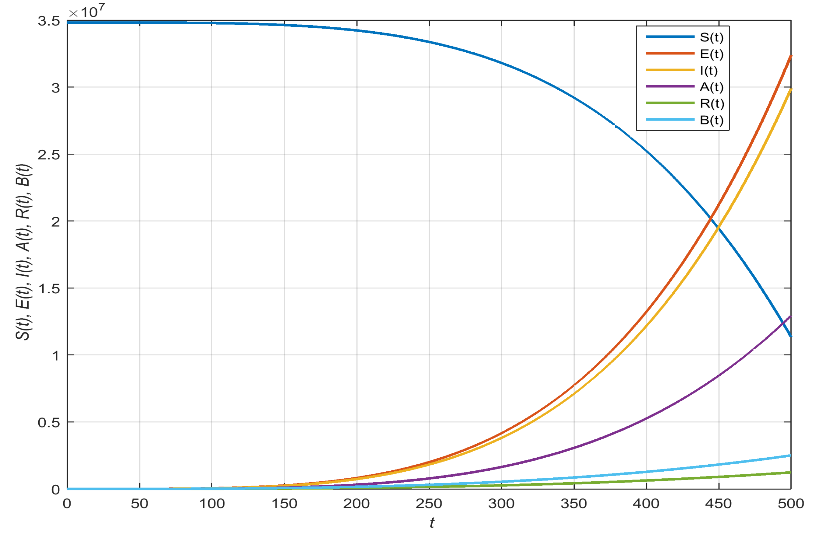
Figure 1. Total population and the concentration of the COVID-19 in the environment.
Axioms 13 00311 g001
Figure 2. The impact of β 1 on susceptible people.
Axioms 13 00311 g002
Figure 3. The impact of β 2 on susceptible people.
Axioms 13 00311 g003
Figure 4. The impact of β 3 on susceptible people.
Axioms 13 00311 g004
Figure 5. The impact of β 4 on susceptible people.
Axioms 13 00311 g005
Figure 6. The impact of β 1 exposed people.
Axioms 13 00311 g006
Figure 7. The impact of β 2 exposed people.
Axioms 13 00311 g007
Figure 8. The impact of β 3 exposed people.
Axioms 13 00311 g008
Figure 9. The impact of β 4 exposed people.
Axioms 13 00311 g009
Figure 10. The impact of ψ 1 on the concentration of COVID-19 in the environment.
Axioms 13 00311 g010
Figure 11. The impact of ψ 2 on the concentration of COVID-19 in the environment.
Axioms 13 00311 g011
Figure 12. The impact of ψ 3 on the concentration of COVID-19 in the environment.
Axioms 13 00311 g012
Figure 13. The impact of ϕ on the concentration of COVID-19 in the environment.
Axioms 13 00311 g013
Table 1. Description of parameters for model (1).
ParameterDescription
β 1 Contact rate among exposed and susceptible
β 2 Contact rate among infected (symptomatic) and susceptible
β 3 Contact rate among infected (asymptomatic) and susceptible
β 4 Contact rate among environment and susceptible
ψ 1 Virus contribution due to E to B
ψ 2 Virus contribution due to I to B
ψ 3 Virus contribution due to A to B
d 1 Natural death rate due to infection at I
Λ Recruitment rate
dNatural mortality rate
δ Incubation period
τ Incubation period
γ 1 Recovery from I
γ 2 Recovery from A
ϕ Virus removal from environment
Table 2. Absolute error using step size h = 0.1.
t e S e E e I e A e R e B
0000000
0.51.6168420991.92 × 10−73.10 × 10−62.35 × 10−64.99 × 10−61.06 × 10−5
13.2336926164.23 × 10−55.34 × 10−55.41 × 10−66.64 × 10−50.000254454
1.54.8507168220.0003568770.0002395446.51 × 10−50.000420680.00180683
26.4683161010.0015184560.0006210710.0002786230.0016410220.007297106
2.58.0872101110.0045669270.0011532620.0008346990.0047727350.021466895
39.7085000350.0110966960.0016182250.0020342790.0114521790.051608136
3.511.333716980.0233239990.0015631290.0043151380.024009710.107905772
412.964858960.0441368980.0002454440.008274570.0455584650.203704952
4.514.604418840.077132070.0034150460.0146902230.0800705010.355718662
516.255405470.1266415640.010877920.0245389760.1324417610.584188452
5.517.921359410.1977519820.0240180220.0390138690.2085472730.913008351
619.606364620.2963179740.0451561820.0595391810.3152878781.369819985
6.521.31505710.4289715050.0770853370.0877837560.460629641.9860852
723.0526310.6031280030.1230926260.1256727240.6536369972.797141232
7.524.824843090.8269902390.1869779750.175397750.9045005433.842242332
826.638015911.1095505640.2730696760.2394259731.2245602865.164590951
8.528.499039761.4605920060.3862373650.3205077631.6263250316.811360906
930.415374151.8906885620.5319028210.4216834322.1234885418.833714418
9.532.395048662.4112049630.716048890.5462890312.73094295211.28681449
Table 3. Absolute error using step size h = 0.01.
t e S e E e I e A e R e B
0000000
0.050.1616852881.60 × 10−71.94 × 10−83.17 × 10−71.81 × 10−72.25 × 10−8
0.10.3233703152.98 × 10−72.76 × 10−86.21 × 10−73.80 × 10−79.60 × 10−8
0.150.4850550744.21 × 10−73.41 × 10−89.12 × 10−76.02 × 10−72.37 × 10−7
0.20.646739585.33 × 10−76.00 × 10−81.19 × 10−68.63 × 10−74.81 × 10−7
0.250.8084238256.33 × 10−71.38 × 10−71.45 × 10−61.18 × 10−68.90 × 10−7
0.30.9701078317.10 × 10−73.10 × 10−71.70 × 10−61.58 × 10−61.56 × 10−6
0.351.1317916217.44 × 10−76.28 × 10−71.92 × 10−62.11 × 10−62.64 × 10−6
0.41.293475247.03 × 10−71.15 × 10−62.11 × 10−62.81 × 10−64.33 × 10−6
0.451.455158715.39 × 10−71.95 × 10−62.26 × 10−63.74 × 10−66.89 × 10−6
0.51.6168420911.89 × 10−73.10 × 10−62.35 × 10−64.99 × 10−61.06 × 10−5
0.551.7785254574.26 × 10−74.68 × 10−62.36 × 10−66.66 × 10−61.60 × 10−5
0.61.9402088671.41 × 10−66.77 × 10−62.29 × 10−68.84 × 10−62.35 × 10−5
0.652.1018924192.88 × 10−69.47 × 10−62.10 × 10−61.17 × 10−53.37 × 10−5
0.72.2635762324.98 × 10−61.29 × 10−51.76 × 10−61.54 × 10−54.73 × 10−5
0.752.425260417.89 × 10−61.71 × 10−51.24 × 10−62.00 × 10−56.51 × 10−5
0.82.5869451021.18 × 10−52.22 × 10−55.18 × 10−72.59 × 10−58.81 × 10−5
0.852.7486304791.69 × 10−52.82 × 10−54.62 × 10−73.32 × 10−50.000117264
0.92.9103167212.35 × 10−53.54 × 10−51.74 × 10−64.21 × 10−50.000153809
0.953.072004023.19 × 10−54.38 × 10−53.37 × 10−65.31 × 10−50.000199056
Table 4. Absolute error using step size h = 0.001.
t e S e E e I e A e R e B
0000000
0.0050.0161685351.73 × 10−82.45 × 10−93.24 × 10−81.76 × 10−82.14 × 10−10
0.010.0323370773.44 × 10−84.81 × 10−96.47 × 10−83.52 × 10−88.62 × 10−10
0.0150.0485056125.11 × 10−87.05 × 10−99.68 × 10−85.30 × 10−81.95 × 10−9
0.020.0646741396.75 × 10−89.19 × 10−91.29 × 10−77.10 × 10−83.48 × 10−9
0.0250.0808426748.36 × 10−81.12 × 10−81.61 × 10−78.90 × 10−85.47 × 10−9
0.030.0970112019.95 × 10−81.31 × 10−81.92 × 10−71.07 × 10−77.92 × 10−9
0.0350.1131797281.15 × 10−71.49 × 10−82.24 × 10−71.26 × 10−71.08 × 10−8
0.040.1293482481.30 × 10−71.65 × 10−82.55 × 10−71.44 × 10−71.42 × 10−8
0.0450.1455167611.46 × 10−71.80 × 10−82.86 × 10−71.63 × 10−71.81 × 10−8
0.050.1616852811.60 × 10−71.94 × 10−83.17 × 10−71.81 × 10−72.25 × 10−8
0.0550.17785381.75 × 10−72.07 × 10−83.48 × 10−72.00 × 10−72.73 × 10−8
0.060.1940223131.89 × 10−72.18 × 10−83.79 × 10−72.20 × 10−73.27 × 10−8
0.0650.2101908182.04 × 10−72.29 × 10−84.10 × 10−72.39 × 10−73.86 × 10−8
0.070.2263593152.18 × 10−72.38 × 10−84.40 × 10−72.58 × 10−74.51 × 10−8
0.0750.242527822.32 × 10−72.46 × 10−84.71 × 10−72.78 × 10−75.21 × 10−8
0.080.2586963182.45 × 10−72.53 × 10−85.01 × 10−72.98 × 10−75.97 × 10−8
0.0850.274864832.59 × 10−72.60 × 10−85.31 × 10−73.18 × 10−76.78 × 10−8
0.090.2910333132.72 × 10−72.66 × 10−85.61 × 10−73.38 × 10−77.66 × 10−8
0.0950.307201812.85 × 10−72.71 × 10−85.91 × 10−73.59 × 10−78.59 × 10−8
Disclaimer/Publisher’s Note: The statements, opinions and data contained in all publications are solely those of the individual author(s) and contributor(s) and not of MDPI and/or the editor(s). MDPI and/or the editor(s) disclaim responsibility for any injury to people or property resulting from any ideas, methods, instructions or products referred to in the content.