Abstract
This manuscript describes the computational process to calculate an airplane path and display it in a 2D and 3D coordinate system on a computer screen. The airplane movement is calculated as a function of its dynamic’s conditions according to physical and logical theory. Here, the flight is divided into maneuvers and the aircraft conditions are defined as boundary conditions. Then the aircraft position is calculated using nested loops, which execute the calculation procedure at every step time (Δt). The calculation of the aircraft displacement is obtained as a function of the aircraft speed and heading angles. The simulator was created using the C++ programming language, and each part of the algorithm was compiled independently to reduce the source code, allow easy modification, and improve the programming efficiency. Aerial navigation involves very complex phenomena to be considered for an appropriate representation; moreover, in this manuscript, the influence of the mathematical approach to properly represent the aircraft flight is described in detail. The flight simulator was successfully tested by simulating some basic theoretical flights with different maneuvers, which include stationary position, running along the way, take off, and some movements in the airspace. The maximum aircraft speed tested was 120 km/h, the maximum maneuver time was 12 min, and the space for simulation was assumed to be without obstacles. Here, the geometrical description of path and speed is analyzed according to the symmetric and asymmetric results. Finally, an analysis was conducted to evaluate the approach of the numerical methods used; after that, it was possible to confirm that precision increased as the step time was reduced. According to this analysis, no more than 500 steps are required for a good approach in the calculation of the aircraft displacement.
Keywords:
flight simulator; programming algorithms; calculation of aircraft position; graphical display of aircraft path; 3D computer animation; numerical approaching MSC:
00A71; 00A72
1. Introduction
The flight of an airplane is a very complex problem; there are many factors and variables involved. Some of these factors depend on human and external factors such as the route of the flight, the pilot’s ability, the geography of the terrain, the weather, etc. Some of these factors depend on the aircraft’s features, such as its speed and aerodynamic design [1,2,3,4,5]. Moreover, aeronautical has always been one of the pioneer industries in developing new technologies to increase performance and improve designs [5,6,7]. Consequently, authors in this area have worked on creating flight simulators, especially in order to reduce costs for training pilots, operational times, and risks [3,4,5,6,8,9,10,11,12,13]. Simulation is a huge area in aeronautics due to not only the flight can be simulated [7,8,9,10,11,14,15,16,17,18,19,20], there are some situations and conditions can vary or can be represented computationally such as flying operations, marketing, programming of routes, design of mechanical compounds etc. [3,4,5,6,7,12,13,14,15,16,21,22,23,24,25,26,27]. Other authors have worked on creating flight simulators, especially in order to reduce costs for training pilots, operational times, and risks [6,7,8,9,10,21,22,23,24,25,26]. The use of physical and computer simulations is desirable not only for training pilots; but, also to evaluate their performance and certification [13,14,15,16,23,24,25,26,27,28,29,30]. Thus, many authors have developed and programmed flight simulators in order to reproduce situations that happen during real flights and other complex problems in aeronautics, aerodynamics and aerial navigation [1,2,3,12,13,14,15,27,28,29,30,31,32,33].
Many of the aeronautical engineers developed physical flight simulators that reproduced some of the basic aircraft navigation instruments [5,6,7]. Their efforts were driven to create functional cabins where pilots could be trained, and they learned what to do in certain situations. As time went on, the aeronautical industry became interested in electronic and computer sciences; aeronautical engineers were pioneers in incorporating these technologies into airplanes [6,7,8,9,10,11,14,15,16,17,18]. Then, with the increase in computer capacities such as data speed management and storage, the improvement in programming methods and techniques has made it possible to develop more complex algorithms and computer simulators for flying [5,6].
Bruce Artwick [7,8,9,10,14,15,16,17] created the first consumer flight simulator software. His original work for Apple II software was purchased by Microsoft and eventually became Microsoft Flight Simulator. Artwick founded the company SubLogic after graduating from the University of Illinois at Urbana-Champaign in 1977, which released the first version of Flight Simulator the following year. Artwick worked for Hughes Aircraft in Culver City, California. It was here that he realized he could create his own 3D dynamic graphics on 6800-based machines. In his thesis of May 1975, called “A versatile computer generated dynamic light display” he showed a model of the flight of an aircraft on a computer screen [8,9,10,11,18,19,20,21,22,23]. With this, Artwick proved that it was possible to use the 6800 processor, which was the first available microcomputer, to handle the graphics and calculations of the specifications needed to create a real-time flight simulation [1,2,3,5,6,7,8].
The algorithms for representing an aircraft flight described in this work are based on the calculation as a single particle under certain speed and time of application conditions; these are so elementary, but they are a platform for including more complex integrations and calculations during an aircraft flight, such as the influence of the wind, the mechanical and aero-dynamical forces, the post-representation of the aircraft position in a virtual environment, etc.
2. Basic Assumptions and Reading Data
In this research, the aircraft flight is treated as an ideal set of planned operations in an ordered sequence. Then the flight is divided into maneuvers and the control variables are aircraft flying conditions such as the aircraft speed, heading angles, and defined times. Then a maneuver is assumed to be the defined group of airplane conditions to be executed during a period of time; thus, a change or remaining on any condition at any time defines the beginning and ending of a maneuver [10,11,12,13,14,15,18,19,20,24,25,26,27,28,29,30]. Nevertheless, there is a minimum of information required that defines the original aircraft status at the beginning of the simulation [24,25,26,34,35,36,37,38,39,40,41].
The general information about the aircraft is the divisions (steps) for analyzing the flight and the maximum takeoff weight (MTOW), which is defined as the aircraft weight at the beginning of the simulation. Thus, a volume for the fuel deposit must be declared according to the following restrictions:
- (a)
- The fuel weight cannot be equal or minor to zero (Vtank ≤ 0).
- (b)
- The fuel weight cannot be equal or major to the MTOW (Vtank ≥ MTOW). This is a basic logical assumption. Here, fuel capacity of tank must be input in (I).
Then a specific fuel consumption rate is defined in (l/km) or (l/min). This consumption is assumed to be constant during the flight simulation; at least a consumption coefficient as a function of the cruise speed was defined. All restrictions were programmed using sentences (if) verifying and conditioning the reading data process [6,7,8,9,10,29,30,31,32,33,42].
All the corresponding warnings were programmed in order to avoid errors during reading data; if any of these restrictions occur, a window with an appropriate message is displayed with a brief explanation in order to correct them [1,2,3,6,7,8,9,27,28,29,30,31,32]. Then, the following assumptions were programmed and included to simulate the flights.
- (1)
- Only one single flight is simulated.
- (2)
- The simulation begins at the initial time (tsim = 0).
- (3)
- The simulated flight is divided into maneuvers (using an integer data type).
- (4)
- The information about every maneuver is used as boundary conditions for the aircraft conditions.
- (5)
- The maneuvers defined cannot be equal or minor to one (n ≤ 1).
- (6)
- The initial conditions for beginning the simulation are established in maneuver (0). For simulations in this work, the airplane was defined as being in stationary conditions.
- (7)
- The times for maneuvers cannot be equals or minors to zero (tn ≤ 0).
- (8)
- The values defined for every maneuver are modified at every step time (t + Δt) according to the previous values until they reach the latest; then, the change is not instantaneous; it is performed step by step during every maneuver.
- (9)
- The aircraft speed is assumed to be in the same direction as the aircraft heading angle. Thus, the aircraft speed is a result of the total propulsion force.
- (10)
- The aircraft with an initial speed equal to zero (vAn=0 = 0) is considered to be in repose or stopped on the ground.
- (11)
- The vertical aircraft speed is assumed to be absolute in the same direction as the pitching angle.
- (l2)
- The values for every maneuver, such as heading angles or aircraft vertical speed, can adopt positive or negative values without restrictions, with the exception of the aircraft speed.
A computational array is used to store and order the information about every maneuver. The array was defined as: Matdat [a][b]; this matrix stores floating data types for all the maneuvers. The location occupied by the variable [a] is used to store and identify the maneuver [a = n]. This location is also used to validate and take the appropriate values during simulation. The location occupied by the variable [b] is used to identify any variable as follows:
Matdat [a][ [b = 1] Horizontal aircraft speed (vHAn).
Matdat [a][ [b = 2] Vertical aircraft speed (vVAn).
Matdat [a][ [b = 3] Heading angle (αn).
Matdat [a][ [b = 4] Rolling angle (αheading).
Matdat [a][ [b = 5] Maneuver time (tn).
In addition, the locations for the variables [b] are also predefined as a matrix with extra locations for storing all of the calculated variables after the execution of the calculation process. Here, the sub-indexes (n) refer to the corresponding maneuver.
The first step in developing a flight simulator is to create a virtual environment on the computer screen where the user can appreciate the aircraft path [1,2,3,4,7,8,9,10,34,35,36,37,38,39,40,41]. The aircraft movement must be represented appropriately, and physical and mathematical equations must be solved using the programming of numerical methods. Several authors have developed methods for solving geometrical and mathematical problems using repetitive operations and procedures [3,4,5,6,9,10,11,12,13,27,28,29,30,31,32,33,42]. This kind of problem can be easily programmed using any programming language. Here, code was generated using C++, and nesting numerical procedures were to be solved [29,30,31,32,33,34,39,41].
Time, aircraft speed, and angular positions during every maneuver are used as initial and final conditions to create a simulation of the aircraft’s animation, and the resulted information is used as input to create an animation of the movement as would be in the aeronautical instruments [29,30,31,37,38,39,40,41]. Then, in this work, the main procedure is a calculation routine that contains the equations for calculating the aircraft displacement along the 3D position. These are solved at every step time (Δt) inside an executed nested loop using the boundary conditions defined by the user. Then, inside this procedure, are included independent subroutines with the code for calculating the graphical information to represent every aircraft instrument. The procedure is described as follows:
- (a)
- Reading the data included general information about the aircraft conditions and the number of maneuvers during the flight. Then specific speed, time duration, and directional conditions of every maneuver are read.
- (b)
- Options for new reading and modification are valuable tools; after this, different display animations were also programmed.
- (c)
- An algorithm to make the simulation is executed, then a calculation of the aircraft displacement is performed, and the information is used to represent the instrument animation.
- (d)
- Options for saving information are included.
In order to represent a landscape for the flight to be simulated, the following facts were assumed to represent computationally the surface and the flight directions:
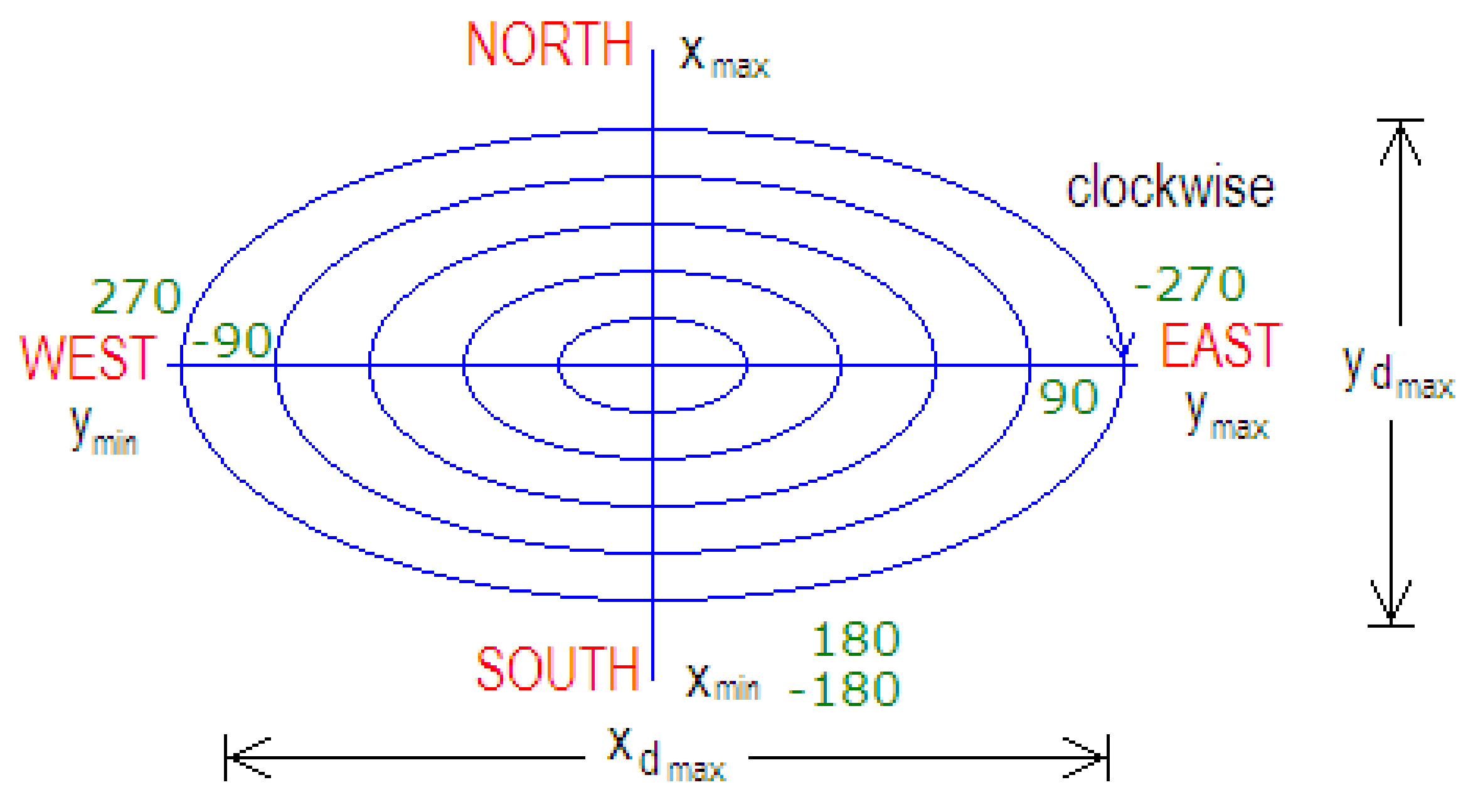
The North Pole corresponds to 0° according to the angular position shown in Figure 1. And the clockwise direction is assumed to be positive to measure any heading angle. Then, 90° corresponds to the east, 180° corresponds to the south, and 270° corresponds to the west; nevertheless, this condition can be modified according to the sense of the turn; for example, −90° can also correspond to the west, −180 to the south, and −270° to the east. This fact is due to the aircraft’s heading angle being taken as a function of its turning movement.
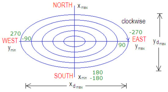
Figure 1.
Assumptions for the graphical representation of the surface and the heading angle (direction of flight) according with earth position.
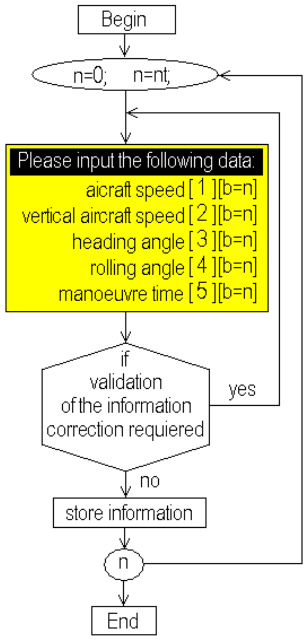
The flow chart shown in Figure 2 represents the general operations of the flight simulator developed. Here, the reading data process is the first action executed. Initially, the general information for the aircraft is read because it is absolutely required to start the calculation process; then the system executes the reading process for the maneuvers. This process appears in better detail in Figure 3, where the procedure to read the data and store it in the computational array is described [3,4,5,6,13,14,15,16,23,24,25,26,27,28,29,30,31,32]. This process is repeated from maneuver (0) until the latest maneuver (nt). In Figure 2, there is a shaded subroutine in the left part. This routine is included to be executed at the beginning to make a pre-calculus about the aircraft flight. The loops and parts of the routines inside are so similar to those in Figure 4a,b. These procedures are so similar, which is why all the procedures were compiled independently and included as separate libraries [27,28,29,30,31,32,33,42]. This fact provides easy identification and modification but also makes them more versatile. The execution time of this subroutine is very short, and its inclusion eliminates the necessity of using additional memory resources or saving unnecessary data. Here (ts) is the simulation time, and the step time (Δt) is calculated as a function of the steps defined to analyze the flight. Finally, the flowchart in Figure 3 shows an option to save the information or quit. The option for saving the information would create a new file named by the pilot (user) and save the data in a row and column format for easy identification.
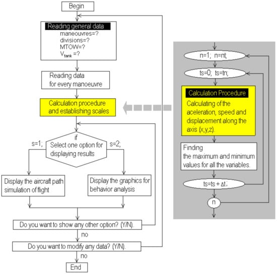
Figure 2.
General flowchart for the flight simulator developed.

Figure 3.
Flowchart for the reading data routine for each maneuver.
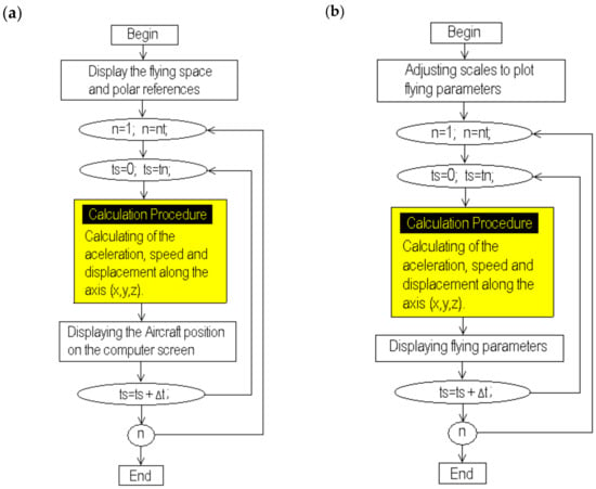
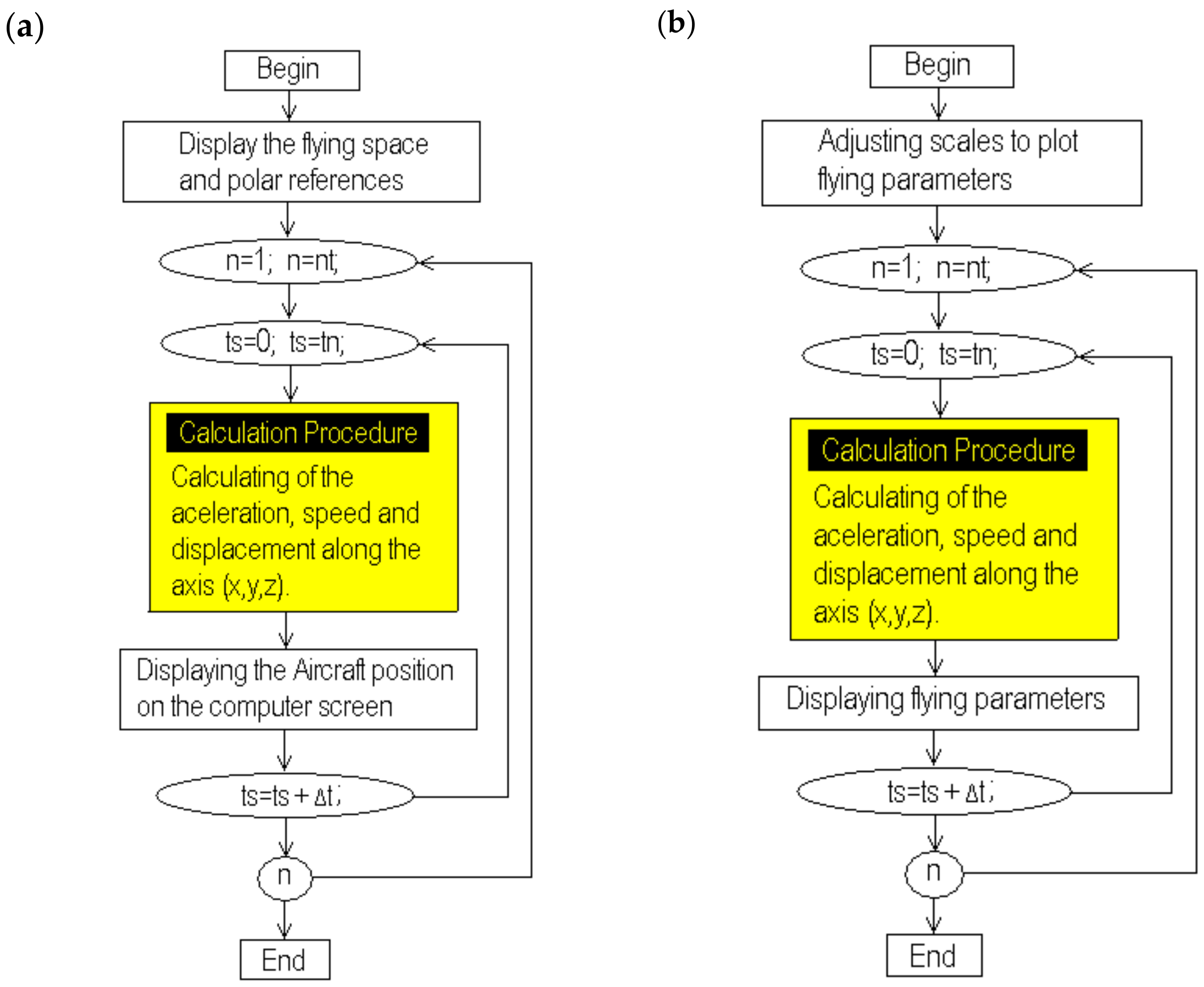
Figure 4.
Flowchart for selecting any option to display the results. (a) Option for display the aircraft path and (b) option for display graphics and performance of the aircraft.
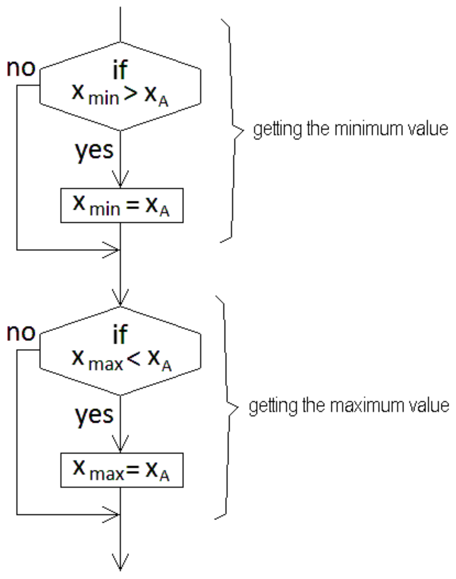
The processes for selecting and displaying the results are shown in the flowcharts in Figure 4a,b. Here, the calculation process is again included during the execution of the simulation loop because it is the same for both options. Each figure indicates the procedure to be executed according to the selection made. In Figure 4a, the virtual aerial space is traced, including the north–south and east–west directions. Then the calculation procedure is executed to display the aircraft path [4,5,6,7,15,16,17,18,19,22,23,24,25,26,27,28,29,30,31]. The flowchart in Figure 4b corresponds to the option developed to analyze the aircraft performance; here, a screen to display the aircraft speed and displacement is drawn according to the calculated scales [27,28,29,30,31,32,33,42]. The routines developed for this purpose were also compiled separately because they are executed many times to display different flight parameters. The flowchart shown in Figure 5 is used to obtain the maximum and minimum values for the displacement of the aircraft along axis (x); a pair of sentences (if) is used for these purposes; the algorithm uses two different comparison procedures that are included in the calculation loop just after the execution of the calculation procedure. This procedure can be repeated for the displacement along the axes (y) and (z); moreover, this procedure can also be nested and used again to compare, obtain, and store the maximum and minimum values of all the variables involved, eliminating unnecessary code.
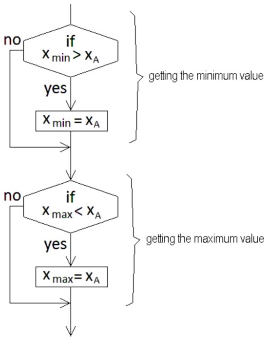
Figure 5.
Flowchart sentence to find the maximum and minimum values for the aircraft displacement along the (x) axis.
The aircraft flight involves the calculation of the 3D aircraft displacement; the calculation is performed in the nested loops as a function of speed and the time conditions defined. Simultaneously, a comparison to obtain the minimum and maximum positions for a good fit with the computer screen pixels resolution is performed [9,10,11,12,13,14,22,23,24,25,26,27,28,29,30,31,32]. All procedures in Figure 2, Figure 3, Figure 4 and Figure 5 were compiled separately in order to be executed independently, and then a quick calculation about the total distances traveled by the aircraft can be obtained. And the display of the displacement is shown only if it is required by the user.
Procedures in shaded areas are nested in the executed loops according to the user requirements; the routine in the flowchart in Figure 5 is also compiled separately and then included during the execution of the nested loops. It is absolutely required to obtain the minimum and maximum values of the aircraft displacement and then draw on the screen the flight; moreover, this procedure is repeated again for the (y) and (z) axes, which are also necessary for it.
3. Calculation Procedure
The calculation procedure involves the solution of the equations for calculating the aircraft path, as described next:
The time of a flight results from the sum of all the partial maneuver times, as shown in Equation (1). Here (n) is the maneuvers, (tn) is the time of every maneuver, and (nt) is the number of maneuvers.
According to Equations (2) and (3), the values of displacement and acceleration can be obtained as a function of the aircraft speed. Here, the super indexes (n) and (n − 1) correspond to the latest and previous maneuvers, respectively.
These equations treat the problem using general assumptions; nevertheless, it is necessary to calculate the displacement and acceleration for every reference axis (x, y, z) using Equations (4) to (6) and (7) to (9), respectively. These equations can be nested inside a computational loop as a part of the calculation procedure; then, the equations for the aircraft movement (10) and (11) are solved, providing instantaneous values for acceleration and displacement.
In order to solve these equations and calculate the aircraft position at every moment during the simulation, it is necessary to establish a step time (Δt) using Equation (12). This value is used as a criterion to determine the precision of the simulation. Here (nt) is the step number, which is an integer data type input by the pilot who runs the simulation. As this number is increased, the step time (Δt) becomes shorter, and the simulation precision improves.
Then Equations (13) to (15) are used to calculate the distances for scaling the aircraft flight on the computer screen.
The distances for the aircraft flight can be obtained from Equations (16) to (18). Equation (16) is the general form of the equation between 2 points in a 3D system; but it must be modified in order to calculate the distance from the starting point to the aircraft at every moment, as is shown in Equation (17); then Equation (18) can be nested in a computer loop to calculate the aircraft displacement.
4. Computer Simulation of Flights
During the flight simulation, the aircraft is placed in the original position (0,0,0) at the initial time (t = 0). Then every maneuver is calculated, and the aircraft position is computed and displayed. A virtual grid terrain is used as a reference for the aerial space where the simulation is executed.
The aircraft path is placed on the computer screen as a function of the transition from a 3D system to a 2D graphical representation. According to this, projected and real paths are displayed in order to provide a complimentary reference. The projected path is that the aircraft is describing over flat terrain, and the real path is that described by the aircraft considering the vertical displacement as a function of the step time (Δt).
Table 1 shows the information declared for the analyzed flights. The flights are 7 and 5 maneuvers; (vhor) and (vvert) are the horizontal and vertical speeds of the aircraft, and (α) is the heading angle.

Table 1.
Information for the flights to be simulated (conditions for every maneuver).
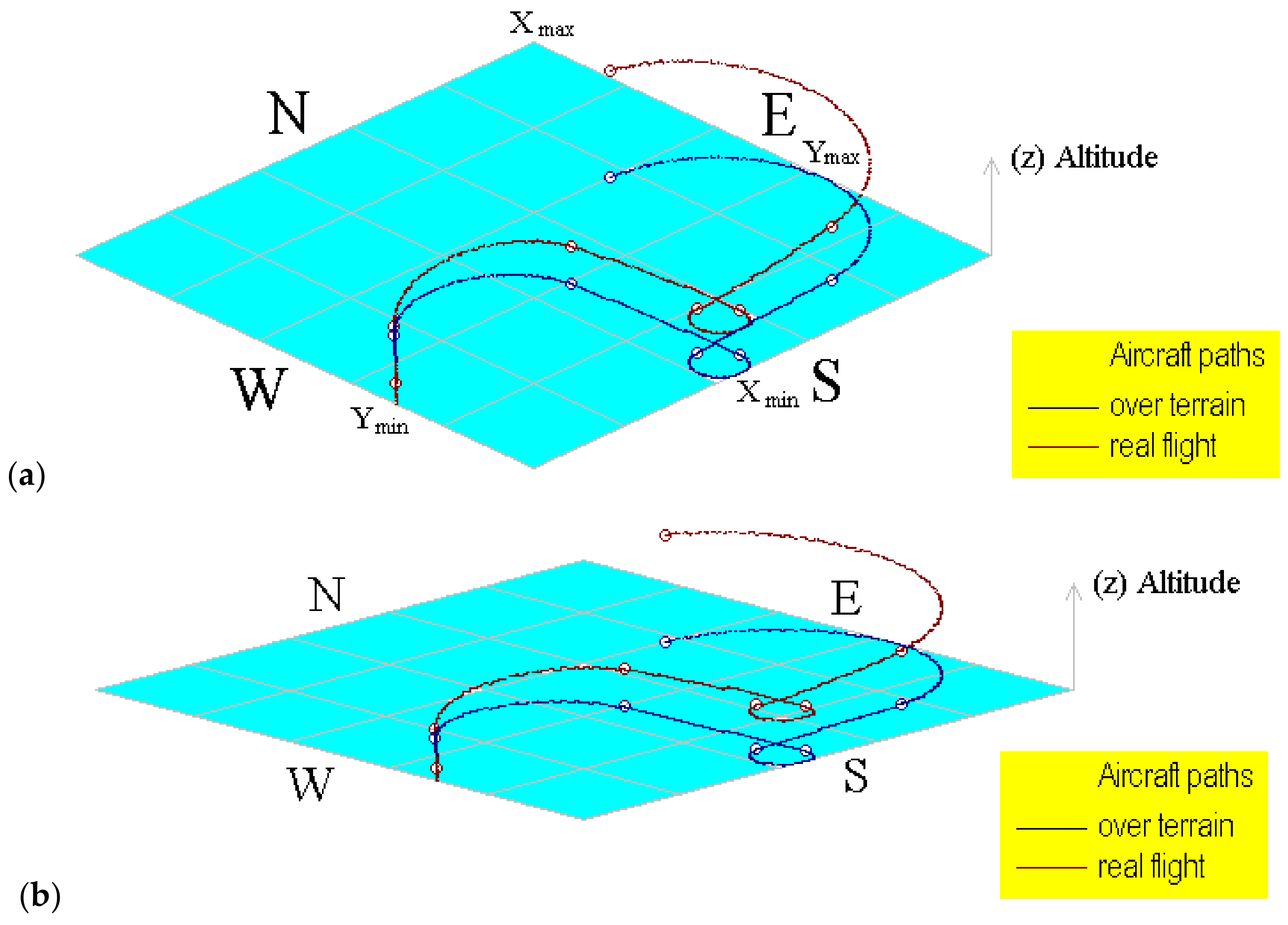
Figure 6a,b shows snapped screens from the simulator. These figures correspond to the flight (1) displayed using different angles over the terrain in order to test the graphical display using rotation and screen scaling tools. These views can be obtained by solving Equations (19) to (21). Here (αterrain) is a reference used to provide an inclined view over the terrain.

Figure 6.
Computational representation of the aircraft path for flight (1) using different terrain angles. (a) Using 20° and (b) using 8°.
Finally, Equations (22)–(24) are used for scaling the aircraft path over the terrain. Here (totpix) is the variable used to display the aircraft path using a congruent scale for the computer screen. Then (npix, npiy and npiz) are the aircraft displacement values expressed in pixels.
A brief description of the flight (1) simulated using the information in Table 1 is explained next; these explanations can be confirmed by watching the aircraft path on Figure 6a,b. Here can be observed the geometrical path in a simulated flat terrain; some maneuvers are symmetrical, but others are non-symmetrical according to speed conditions. The aircraft in this flight is initially placed on the ground at 45° (north–east direction) and then runs over the road and takes off in the same direction and turns to the right (clockwise); maintains a direction towards the south, then turns again to the right and maintains a new direction to the east; finally, turns left to the north and west against clockwise.
The computational tool developed to incline the terrain is very useful and versatile to provide a different point of view of the built aircraft paths. Here, the path over terrain can be easily identified because it is never out of the shaded area.
Maneuver 1. The aircraft is initially in stationary conditions; then it runs in order to prepare for take-off. The aircraft speed changes from (vxn=0 = 0) to (vxn=1 = 100 km/h) at the end of the first maneuver. There are no modifications to the lateral or vertical speed; the aircraft just runs over the reference plane. The heading direction is +45°, which corresponds to 45° measured from the North Pole direction. This run delays 2.50 min.
Maneuver 2. During this maneuver, the aircraft takes off, continues accelerating until it reaches vxn=2 = 120 km/h. Here, the aircraft increases its vertical speed until vzn=2 = 25 km/h. Then the projected and real aircraft paths are separated; the projected path is always traced as a function of the reference plane, and the real path is displayed considering the aircraft altitude over the terrain. This maneuver delays 2.35 min, and the heading angle remains +45°. So, the slope in the line for this segment indicates that the aircraft has taken off from the highway at the same heading angle, describing a line with a smoothed slope.
Maneuver 3. Here the aircraft decelerates slightly until (vxn=3 = 100 km/h); the vertical speed is decreased until (vzn=3 = 5 km/h); nevertheless, the aircraft continues ascending due to the vertical speed value continuing to be positive. Moreover, during this maneuver the aircraft’s heading route is modified from +45° to 180°. So, the original aircraft direction north–east now is towards south. Then the aircraft turns to the right. This maneuver is executed for 6 min, so the advanced distance is longer than those in previous maneuvers.
Maneuver 4. Here the aircraft accelerates slightly again until (vxn=4 = 110 km/h); the vertical speed is nearly invariable (vzn=4 = 0 km/h). In addition, the heading angle remains in a south direction, so the segment of the path for this maneuver is a straight line.
Maneuver 5. Here the aircraft decelerates lightly until (vxn=5 = 100 km/h); the vertical speed becomes negative (vzn=5 = −2.20 km/h); and the aircraft suddenly turns from 180° to 450°, changing the heading route to the east. A turn is quickly performed in 3.25 min, during a light descent. Thus, the path described for this maneuver is a little elliptical arc.
Maneuver 6. The aircraft increases its propulsion and its vertical speed, but the same heading angle remains; so, the aircraft direction also remains towards the east with a slight increment in altitude.
Maneuver 7. Finally, the aircraft speed is slightly decreased, but although the vertical speed is also slightly decreased, the ascending rate remains considerable. Thus, a notorious increment in the aircraft’s altitude can be observed during this maneuver. Moreover, the aircraft changes its heading angle towards the west during the longest period of time.
Speed curves are lines for the initial maneuvers when the aircraft runs along the way, and others are sinusoidal or second-grade curves. Some of these present conditions of symmetry or asymmetry as a function of the aircraft acceleration and the modification of the aircraft direction. In maneuvers 5 and 7, the speed curves are sinusoidal and are inverted for both axes (x, y). This can be considered a partially symmetric or inverted symmetry condition.
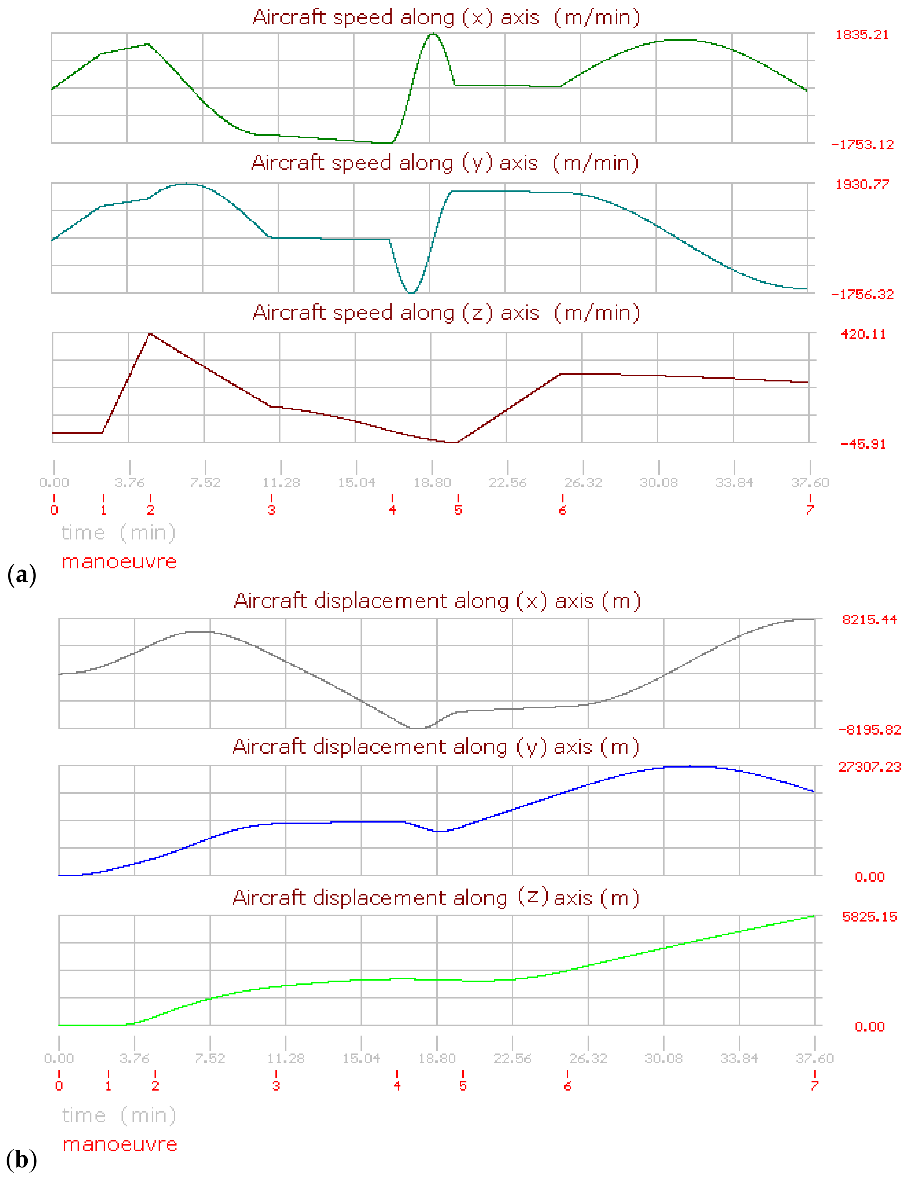
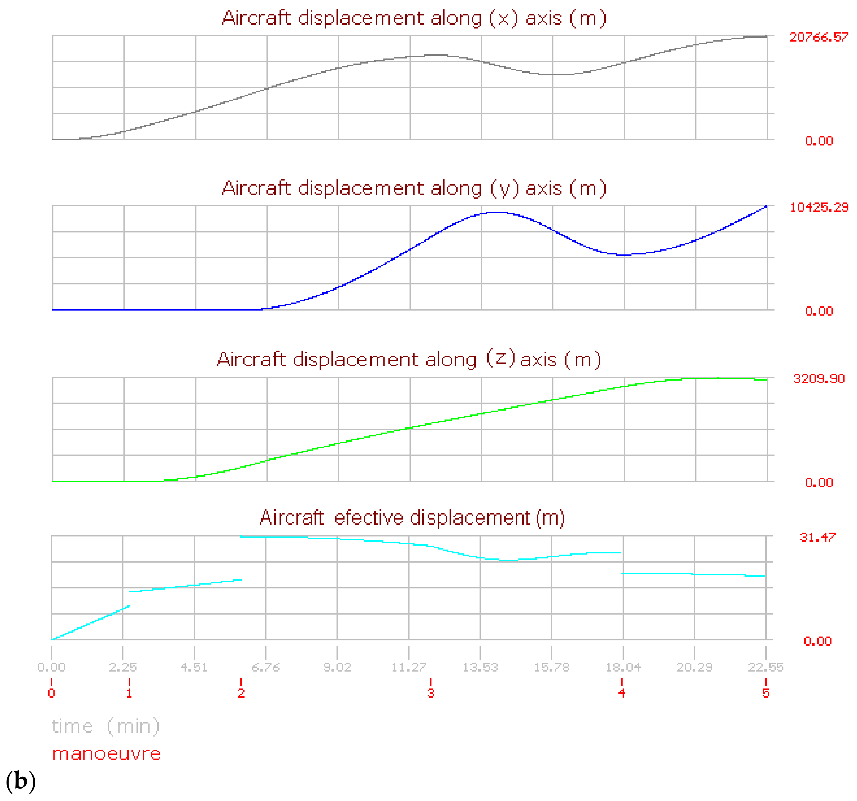
The aircraft performance and behavior during a flight can be analyzed along the axis (x, y, z). Figure 7a,b shows the evolution of the flight (1). Both figures use a dual time scale for the horizontal axis, indicating the maneuver duration just below. The maximum and minimum values are indicated on the vertical axis, which were obtained from the simulation. Figure 7a shows the aircraft speeds for each referred axis; here, the speed on the axis (x) shows the following features:
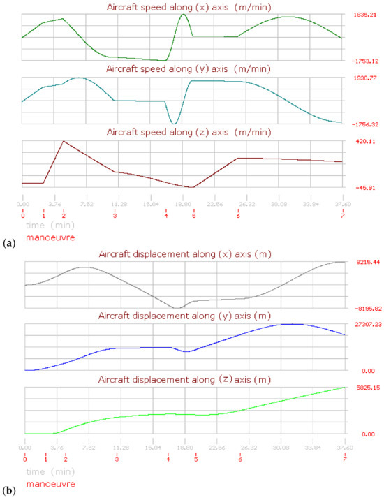
Figure 7.
Aircraft performance graphics for flight (1) (a) Aircraft speed. (b) Aircraft displacement.
The aircraft is initially in a stop position (vzn=0 = 0 km/h). Then the speed is increased until (vzn=1 = 100 km/h) at the end of the first maneuver. Here, a straight line with a constant slope is displayed, evidencing the aircraft’s acceleration. Another line with a minor but constant slope was obtained for the second maneuver due to the increased speed, but at a minor rate. For the third maneuver, the speed curve has a negative slope due to the aircraft having modified its heading route. Then this condition changes the plotting of the speed. During the fourth maneuver, the speed is slightly increased, but with a negative implication, so the slope is nearly horizontal, thus the line with a lightly negative slope can be appreciated. During the fifth maneuver the aircraft’s speed decreased slightly, but it modified its heading direction from 180° to 450°, or from the south to the east, including a quick turn rotation, and the plotting conditions were modified again, resulting in a sinusoidal line segment. During the sixth maneuver the aircraft speed is slightly decreased, but the final plotting position of the fifth remains because the heading angle also remains constant. Finally, during the seventh maneuver, the aircraft changes the heading condition from east to west, becoming the line in this segment with a positive slope until it reaches a maximum value for the North Pole direction; then, the slope becomes negative, forming the end of the curve that corresponds to the final turn position.
The speed curves change geometrically with every maneuver as a function of the simulation conditions. The segments are influenced by the heading angle changes, which modify the direction of the slopes. During flight (1), the heading changes conducted by the aircraft on maneuvers three and five were performed turning towards the right; nevertheless, the final heading changes were performed turning towards the left. Moreover, the maneuver times (tn) also influence the aircraft displacement. So, it is possible to mention the following facts after analyzing the speed curve for the (y) axis:
During the first and second maneuvers the speed behavior is represented by 2 lines with constant slopes in the same way as for the axis (x). Nevertheless, the curve for the third maneuver is very different due to the heading changing from 45° to 180°. Here a maximum is reached for a position east to 90°. Then the curve changes its slope to negative until the end of this maneuver. During the fourth maneuver, the heading remains invariable with a slight increment in the aircraft speed, resulting in a quasi-horizontal line. The aircraft modifies its heading during the fifth maneuver; here a sinusoidal curve is appreciated, but the starting and ending angles are different in comparison with the curve for the speed on the axis (x); the maximum and minimum positions on curves for the analysis over these axes are in mathematical correspondence with the inflection points for the (x) axis. After this, the aircraft remains with a constant heading angle, and for the sixth maneuver, a new sinusoidal curve is shown for the final maneuver due to the heading angle change.
The vertical speed (vz) is very easy to understand due to all the segments being lineal. Here, initially, the aircraft runs over the reference plane (vz = 0); this first maneuver is represented by a horizontal line. During the second maneuver the aircraft takes off; then, the curve has a very vertical positive slope. For the third, fourth, and fifth maneuvers, the vertical speed decreases at different rates, although the aircraft remains always ascending. For the sixth and seventh maneuvers, the vertical speed is increased, but also at a different rate, so the slope changes from positive to negative.
The displacement curves for flight (1) are shown in Figure 7b. Thus, it is possible to mention the following facts about the curve on the axis (x):
The curve begins at an initial speed equal to zero; the displacement curves are different than speed curves due to the displacement rate not being constant (vHA = dHA/dt). During the third maneuver, the displacement reaches its maximum value, and then the slope becomes negative due to the route change. On the fourth maneuver, the heading angle remains unchanged, and the displacement is a line with a negative slope. During the fifth maneuver, the aircraft turns suddenly, changing its heading angle; here, a little inverse curved form with a quasi-flat ending is appreciated. During the sixth maneuver, the aircraft route remains the same; consequently, the curve is lineal. Finally, during the last maneuver, a sinusoidal form is the result of the route change.
Analyzing the curve for displacement on the axis (y), the displacement is similar to the curve for (dx) for the first two maneuvers due to the aircraft speed and acceleration being at the same heading angles. On the third maneuver, the heading angle changes, and the displacement along (y) is lightly decreased. On the fourth maneuver, the effective displacement is increased, but the heading angle is nearly perpendicular to the axis (y), so the displacement about this axis is a horizontal line. During the fifth maneuver, the aircraft turns quickly 270°, turning in the east direction in a short period of time. On the sixth maneuver, the aircraft remains at the same heading angle, resulting in a line with a nearly invariable positive slope. Finally, during the last maneuver, the form of a circular semi-arc is displayed due to the turning again.
The displacement along the vertical axis (z) is shown below. Here, the aircraft begins remaining on the ground during the take-off run. Then the aircraft’s altitude begins to increase during the second maneuver. The aircraft continues increasing its altitude for the next maneuvers, but at different rates, so the slopes are also different. With the exception of the fifth maneuver, which was defined with a negative value. Then it is important to mention that if a negative value is defined on any maneuver for the vertical speed, the aircraft remains ascending until the transition of values becomes negative (vzt+Δt < 0).
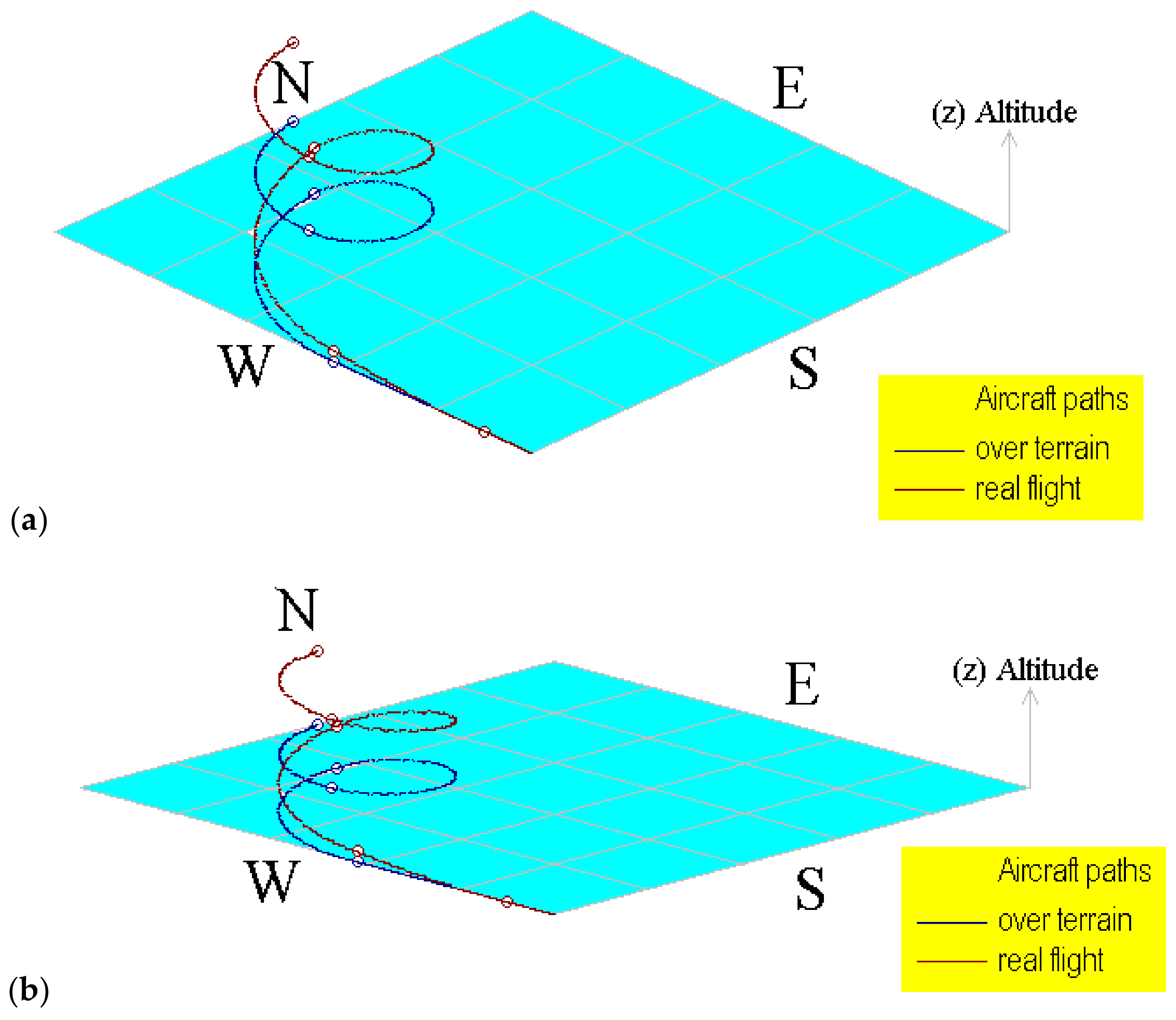
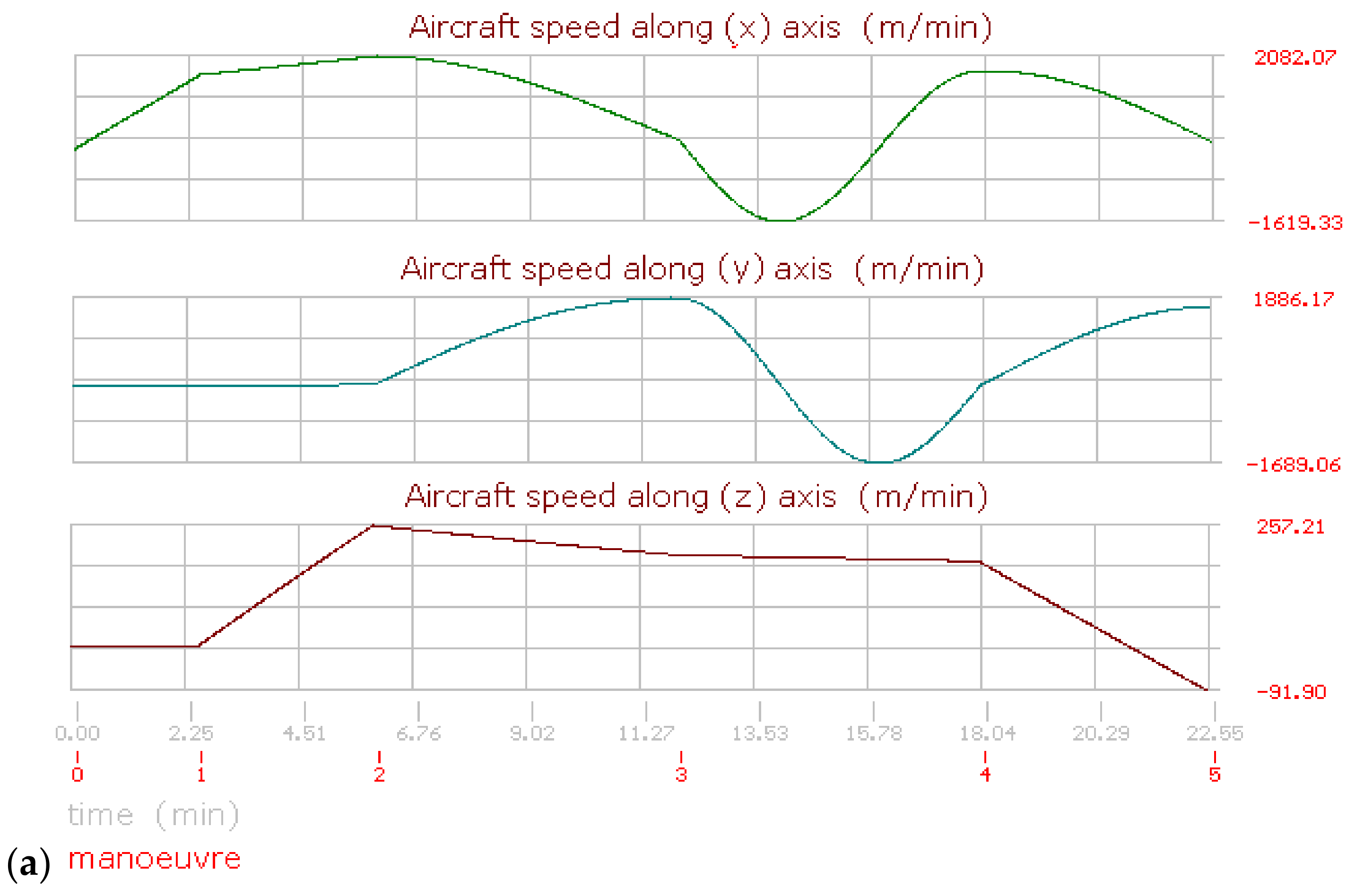
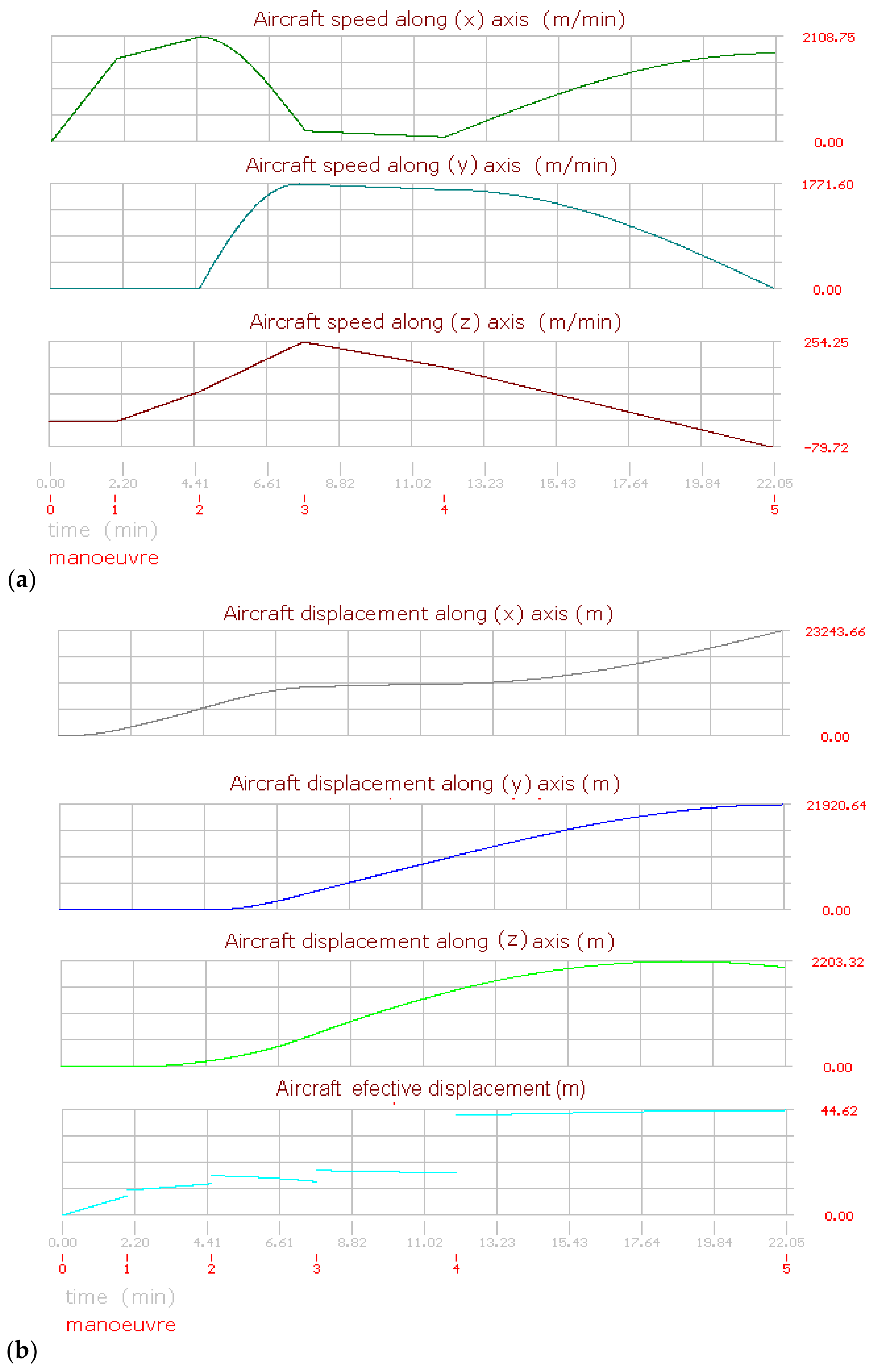
Figure 8, Figure 9, Figure 10 and Figure 11 show the aircraft path, speed, and displacement curves corresponding to the flights (2) and (3), respectively. Here, differences and similarities in comparison with flight (1) can be appreciated. Moreover, the influence of aircraft speed, heading angles, and maneuver times can also be appreciated.

Figure 8.
Computational representation of the aircraft path for flight (2) using different terrain angles. (a) Using 20° and (b) using 8°.
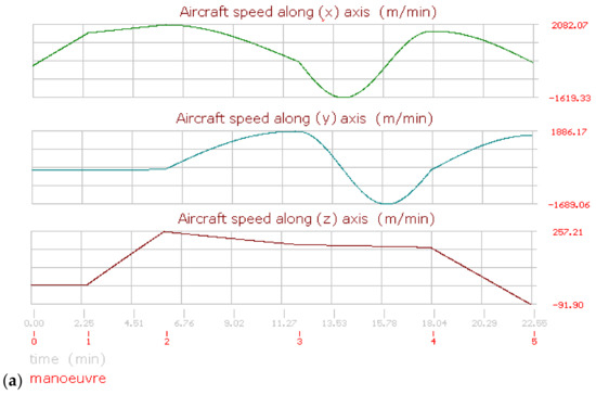
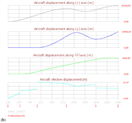
Figure 9.
Aircraft performance graphics for flight (2). (a) Aircraft speed. (b) Aircraft displacement.
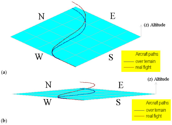
Figure 10.
Computational representation of the aircraft path for flight (3) using different terrain angles. (a) Using 20° and (b) using 5°.
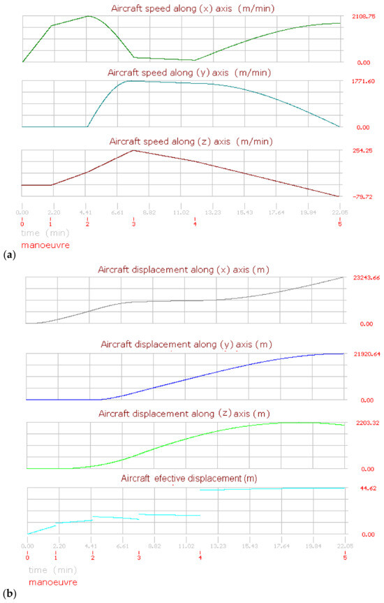
Figure 11.
Aircraft performance graphics for flight (3). (a) Aircraft speed. (b) Aircraft displacement.
The aircraft on this flight is stationary with a direction to the north equal to 0°. Then it runs over the road and takes off in the same direction. On the next maneuver, the heading angles are always greater than the previous; thus, the aircraft always turns to the right in a clockwise direction. Moreover, the vertical speed is positive, the aircraft ascends until the fourth maneuver, and until the last maneuver, the aircraft lightly descends due to the final vertical speed being negative. Figure 8a,b shows the aircraft displacement over different terrain angles for view, evidencing the importance of displaying the flight path.
The flights were divided for analysis purposes into maneuvers with particular conditions of aircraft horizontal and vertical speed; a route angle and time endurance are defined; then the displacement is calculated. Then, all the equations in the manuscript are solved using an integration numerical Runge–Kutta method, which is very easy to program using nested loops with a minimal computational effort. Although increasing the steps for calculation is an easy way, there are some variables involved in the simulation that affect the final approach; therefore, it will be absolutely necessary to increase these in the following cases.
- (a)
- If the aircraft’s horizontal and vertical speeds are increased.
- (b)
- If the endurance time of the maneuver is increased.
Other parameters influence the aircraft route, as follows:
If the heading angle is greater than in the previous maneuver, the aircraft will turn to the right.
- (a)
- If the heading angle is less than in the previous maneuver, the aircraft will turn to the left.
- (b)
- It is important to remember that a simulation is considered precise when a very accurate calculation of the aircraft’s position in space is obtained. Additionally, mathematical and physical theory must be applicable to different conditions with the same certainty.
5. Evaluation of Approaching
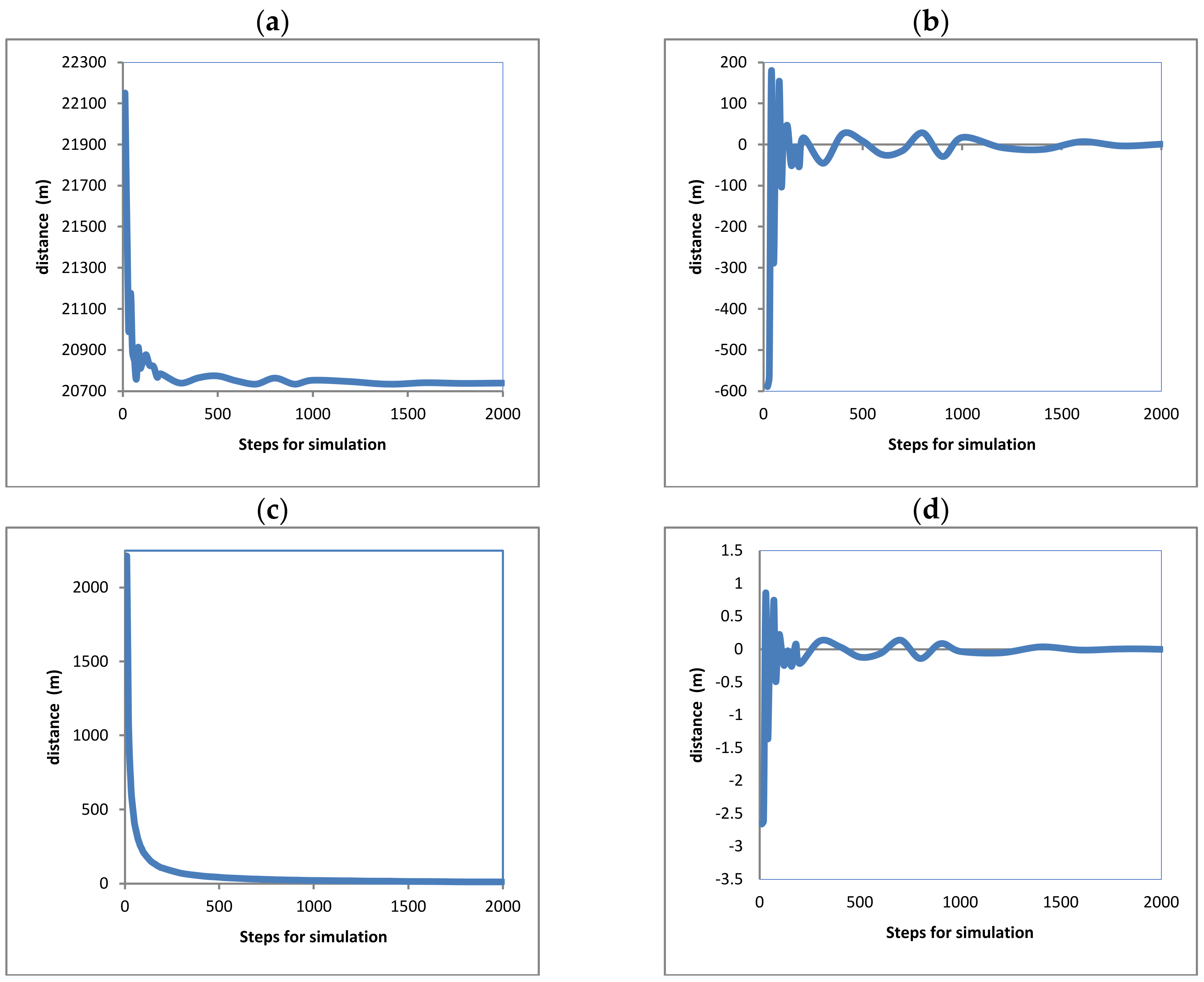
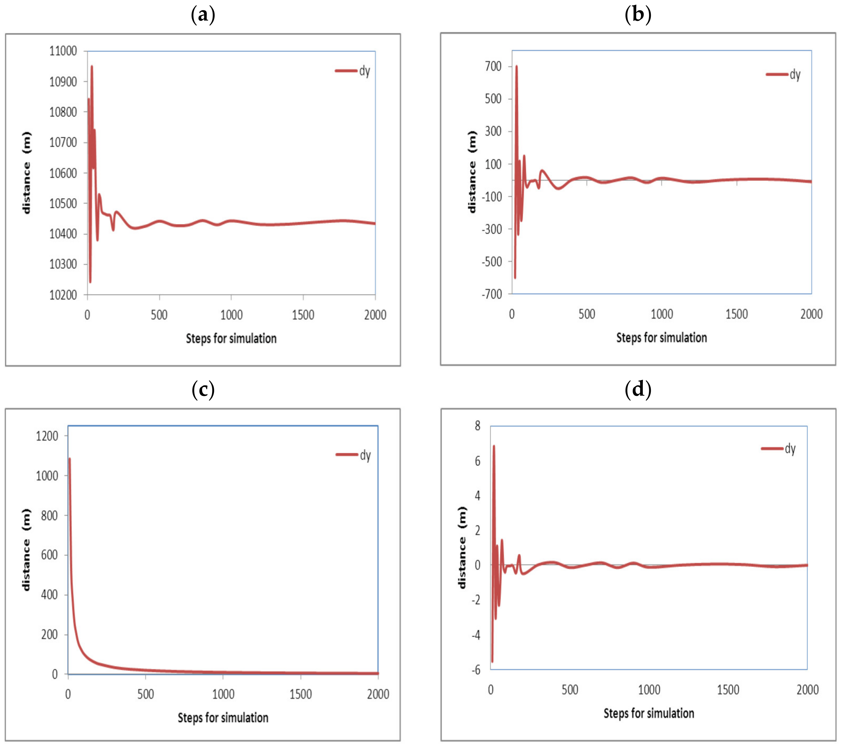
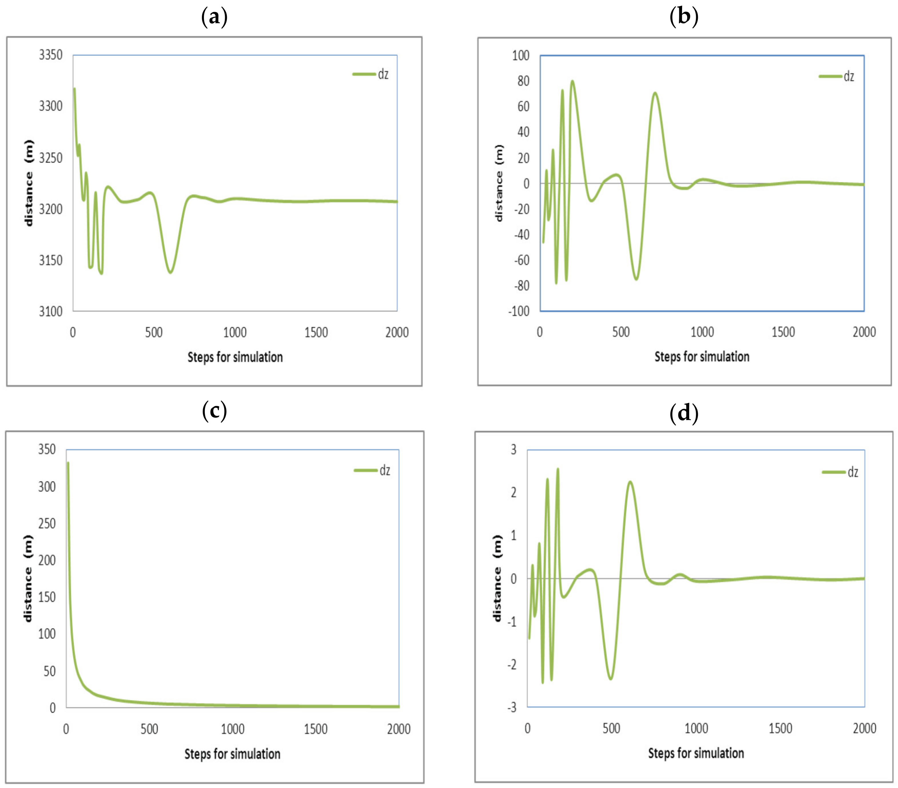
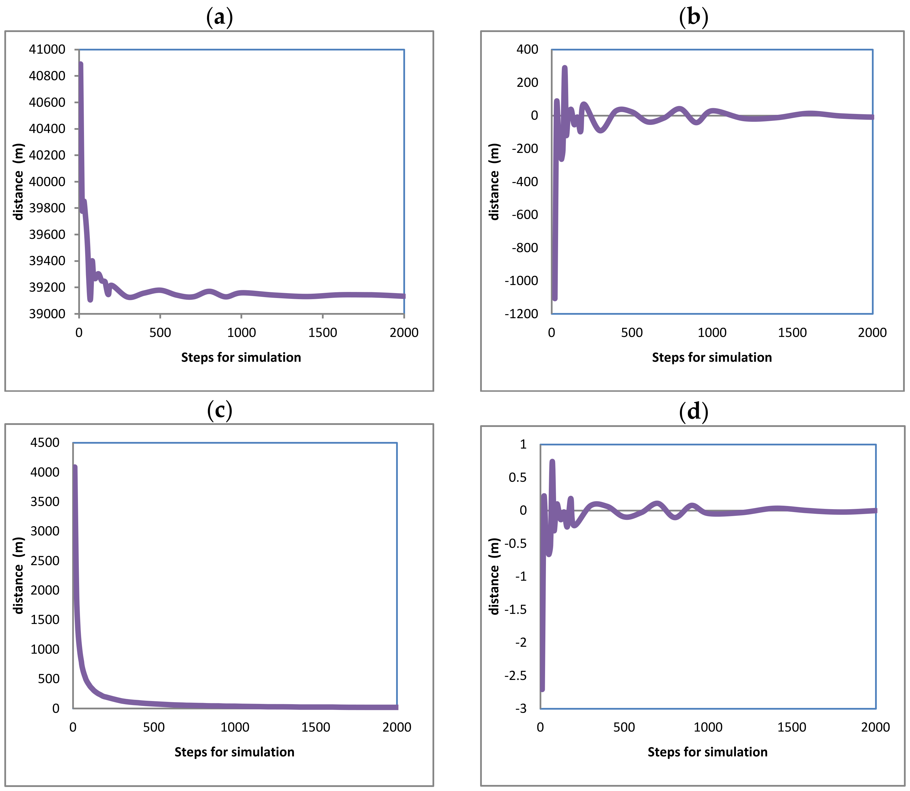
In order to evaluate the numerical method programmed for the simulator, approaches and errors were analyzed by executing the nested routines in the simulator with different divisions (steps) reproducing the 3 flights defined in Table 1. Similar curves resulted for the three flights. The results for flight (2) have been chosen to evidence the error and approaching obtained and are shown in Figure 12, Figure 13, Figure 14 and Figure 15. These curves show the evolution of the final distances calculated for the aircraft path. The distances (dx), (dy), and (dz) are the distances flown along every axis, and (dtot) is the total distance from the origin of the aircraft flight. All of them were measured from the original starting point of the flight, assumed to be the position (0,0,0) towards the corresponding displacement axes. Their description of content is as follows:
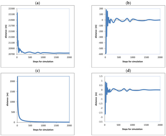
Figure 12.
Calculated approaching for flight (1) curves for axis (x) direction Sud-North. (a) considering displacement values. (b) considering the previous calculated value. (c) considering the division of the displacement between the number of steps. (d) considering the approaching to the final value.
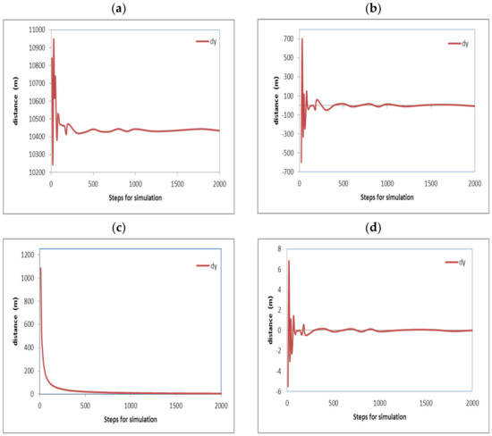
Figure 13.
Calculated approaching for flight (1) curves for axis (y) direction Est-West. (a) considering displacement values. (b) considering the previous calculated value. (c) considering the division of the displacement between the number of steps. (d) considering the approaching to the final value.
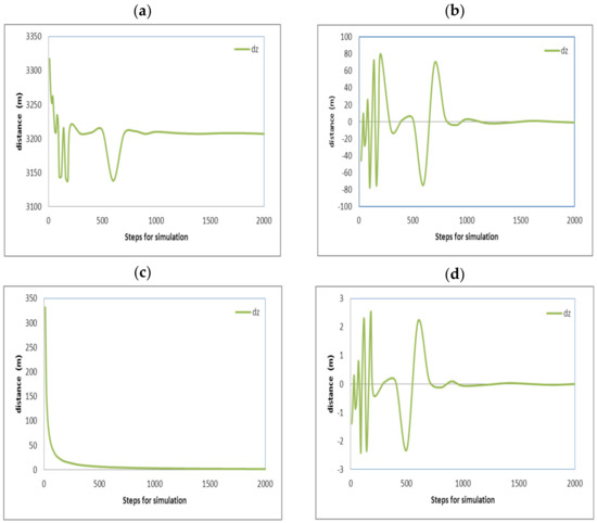
Figure 14.
Calculated approaching for flight (1) curves for axis (z) this is for the altitude. (a) considering displacement values. (b) considering the previous calculated value. (c) considering the division of the displacement between the number of steps. (d) considering the approaching to the final value.
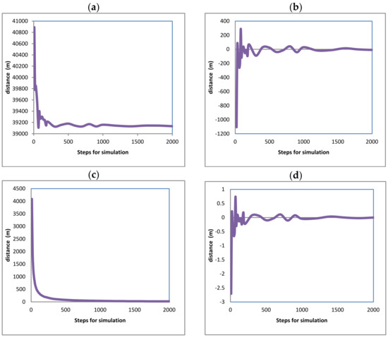
Figure 15.
Calculated approaching for flight (1) curves for total distance measured for the original point assumed as the aircraft was in a stationary position at (0,0,0). (a) considering displacement values. (b) considering the previous calculated value. (c) considering the division of the displacement between the number of steps. (d) considering the approaching to the final value.
Approaching every displacement axis, the total displacement will be described. Figure 12a–d shows the displacement for the (x) axis with different criteria of approaching that are described next; similarly, Figure 13a–d shows the displacement for the (y) axis, Figure 14a–d shows the displacement for the (z) axis, and Figure 15a–d shows the total aircraft displacement, respectively. In all these figures, the values of displacement are plotted as a function of the steps for calculation. But different criteria for approaching are evaluated in order to achieve improvements.
Curves (12a, 13a, 14a, and 15a) show the fluctuation of the displacements along the directions (x), (y), (z), and the total aircraft displacement, respectively, evidencing that the final distances tend to adopt an invariable value. The reduction in this variation indicates that error is reduced and approaching is improved as the steps for analysis are increased.
The vertical axis in Figure 12a, Figure 13a and Figure 15a represents the displacement along the respective axis “x” for direction north–south and “y” for direction east–west and the total displacement. In contrast, the vertical values in
Figure 12b, Figure 13b and Figure 15b are so minor because they were calculated using Equation (25). Additionally, the curves in Figure 12c, Figure 13c and Figure 15c were obtained using Equation (26), and the curves in Figure 12d, Figure 13d and Figure 15d were obtained using Equation (27).
Curves (12b, 13b, 14b, and 15b) show the fluctuation of the values calculated for the distances for the (x), (y), and (z) axes and the total aircraft displacement. Respectively. All these curves tend to zero because the values were obtained from the subtraction of the values with the previous calculation (with steps 1). This also means that the error is reduced as the steps for calculation are increased. The values in these curves were obtained using Equation (25). Here, (dx) is the distance on the axis (x); this equation is also solved again for the (y), (z) axes, and the total distance. The sub-index (ns) refers to the number of steps used for calculation. And the super index (t = total) means that the value corresponds to the latest calculated displacement in the latest step of the latest maneuver; this is at the end of the simulation.
Curves (12c, 13c, 14c, and 15c) show the fluctuation of the values calculated for the distances for axis (x), (y), and (z) axes and the total aircraft displacement, respectively, divided by the steps used, also evidencing that the final values tend to be zero. This means that the error tends to be reduced again. Although these curves tend quickly to zero, they are not considered the best evidence of a good approach. The curves resulted after the application of Equation (26) to the final displacement values calculated; all these curves immediately tend to zero. Nevertheless, this approaching calculation is not the most reliable because (ns) is always increasing; thus, the next value will always be minor.
Curves (12d, 13d, 14d, and 15d) show the fluctuation of the values calculated for the distances for the (x), (y), and (z) axes and the total aircraft displacement, respectively, minus the previous value and divided by the previous value, also evidencing that the final values tend to be zero. This means that the error tends to be reduced again. These curves result from the application of Equation (27). All of these curves tend to zero, but there are positive and negative variations that diminish.
Fluctuations on these curves can be positives or negatives due to the change in heading angles and the steps used for calculation; fluctuations for the axis (z) were major in contrast with the (x) and (y) axes, but they are not according to the scales on the vertical axes.
These curves evidence the following facts for flight (2):
The difference between the displacements calculated tends to a final value; then the error in the calculation is reduced as the number of steps is increased, as could be expected for any integration method; thus, the approaching is improved. The same behavior can be appreciated for every analyzed axis and for the total displacement.
According to the steps used for the calculation of the flights, it is possible to affirm the following facts for all the analyzed axes:
Using 10 to 100 steps, the approaching is bad.
Using 100 to 1000 steps, the approaching is notoriously improved. The fluctuations in the calculated values are damped.
Using 1000 to 2000 steps, the approaching was not significantly improved, which is why it can be considered not absolutely required.
It is important to mention that horizontal aircraft speeds are often higher than vertical speeds, but these can be so different depending on the aircraft type and capacity. For major speeds, it will be necessary to calculate the displacement using more steps.
The maneuver time has a strong influence on the approaching; the increment in steps is the best way to improve approaching for long times.
The aircraft speed also has a strong influence over calculation; increasing the steps for calculation reduces the errors and improves approaching if the aircraft speed is increased, as is appreciated in Figure 12, Figure 13, Figure 14 and Figure 15. Moreover, fluctuations are so high in the vertical axis (z) due to altitude, with minor values in comparison with horizontal displacements. Additionally, it must be noted that a particular approaching can be calculated for every maneuver since everyone has particular data. Nevertheless, for this work, it was decided to do it for the completed flights.
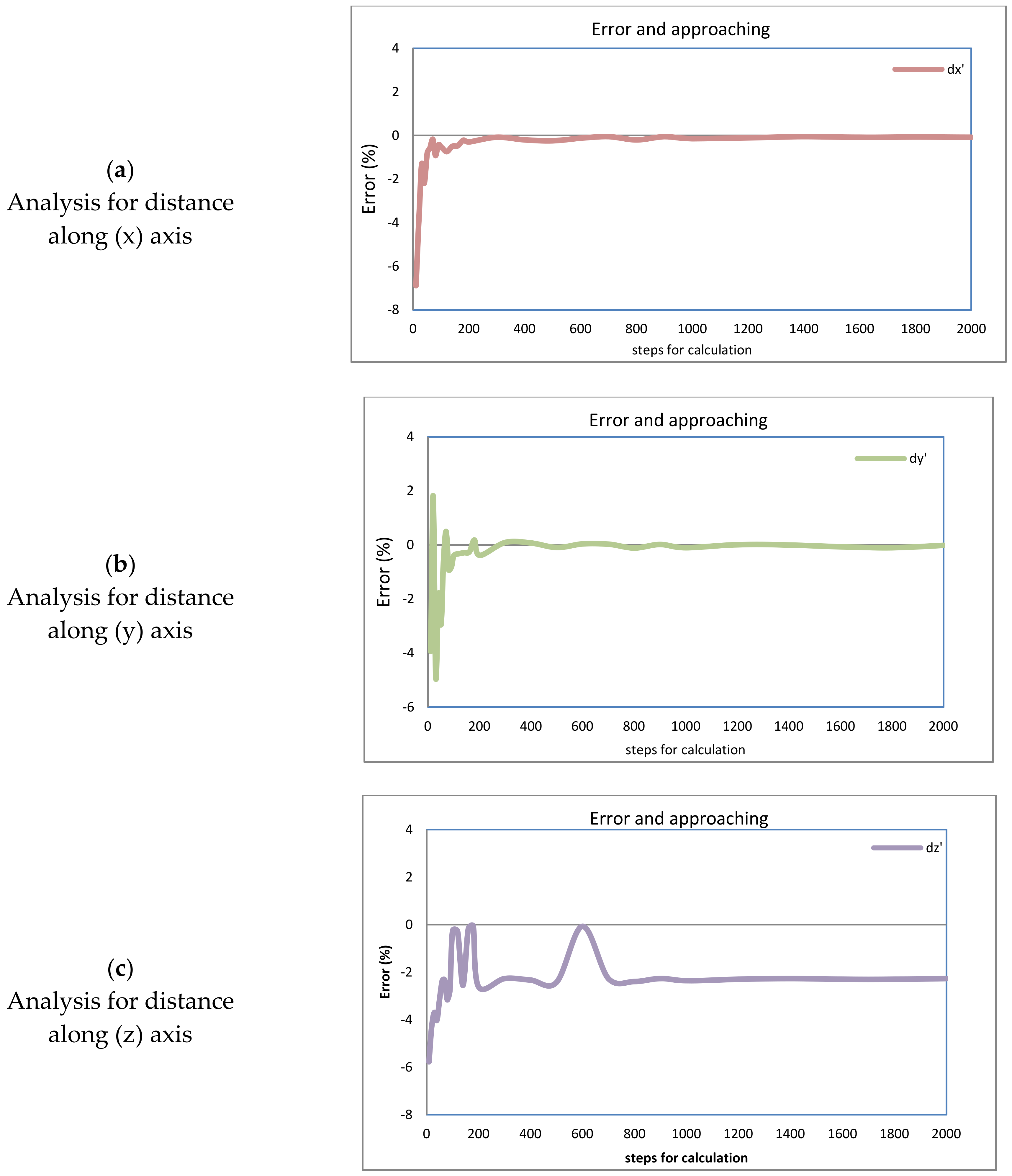
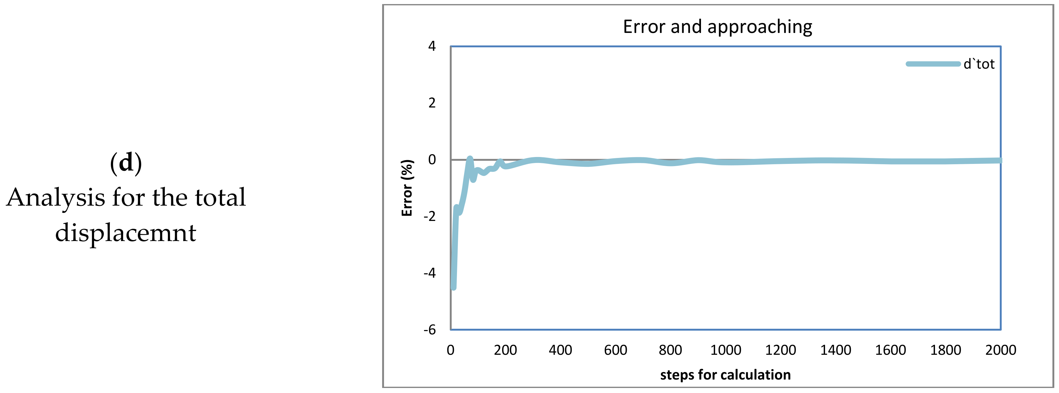
In addition, the displacement values for every flight along the 3 axes and the final displacement using 10,000 steps were calculated, which are considered enough for a very good approaching. The results shown are in Table 2, and additional curves resulted from the application of Equation (28) are shown in Figure 16a–d. The application of these equations shows the approaching as an error in percentage, referring to the value calculated using a large number of steps, and can also be used for comparison.

Table 2.
Calculated distances along the axis (x, y, z) and total measured from the aircraft origin for every simulated flight.
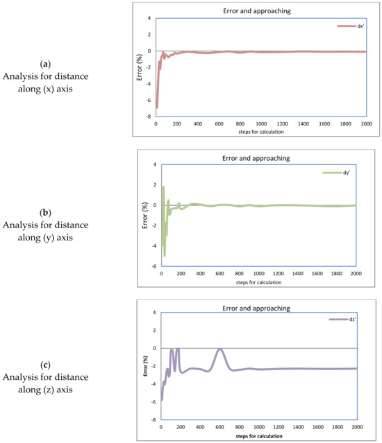
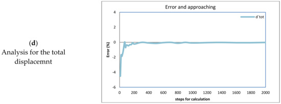
Figure 16.
Reduction in the error calculated for flight (1) over every axis of displacement. Analysis for every displacement calculated (a) for Sud-North direction. (b) for Est-West direction. (c) for altitude. (d) for total displacement.
According to the graph shown in Figure 16a, a good approach is obtained using more than 400 steps for analysis because it tends to zero with such minimal variation. Maximum variations are from (−7.2%) when less than 100 steps are used. In the case of the direction east–west on axis (y), there is a similar damping behavior as the steps are increased, but at the beginning, variations are positive and negative. The maximum variations are between (−4%) and (2%). Although, in the same way as for axis (x), both curves tend to a final true value with a variation almost equal to zero. Thus, it can be considered that the variation over 400 steps is not so significant, and the solution is so close to the real, final true values. In the axis (z) for the altitude where the aircraft is flying, there is a variation until 800 steps; moreover, for 2000 steps, there is a variation of (2%). This variation is considerable, but it must be taken into account that the distance over this axis is so minor in comparison with the distances on the axes (x) and (y) and over the total distance. In Figure 16d, the same behavior is observed, and the curve is so similar to those in Figure 16a,b, evidencing the stronger influence of the much longer distances traveled on the horizontal axes as was shown in the flight path.
6. Discussion
According to the results obtained, it is possible to affirm that any aircraft flight condition can be properly calculated and represented computationally with the algorithm developed. Moreover, the approaching calculation can be easily improved by increasing the number of calculation steps. In addition, no more than 500 steps are needed for a good approach, although for different speeds and times of maneuvers, approaching analysis must be performed; this work can be quickly carried out with a minor computational effort. For immediate future studies, the information calculated can be employed to represent the aircraft instrument animation in a virtual environment to develop a more complex simulator. Some of the potential topics that can be developed from this work are the following:
- (a)
- Computational representation of the aircraft instruments can be employed to train pilots or just to show students and enthusiasm their function described with theoretical support.
- (b)
- Planning of aircraft flights and representation of flights in a basic virtual environment, including obstacles such as a defined geography for terrain. This option can provide tools for planning operations with safe air flying conditions.
- (c)
- More complex calculations, including wind components or weather conditions, influence the aircraft path and the calculation of forces to correct.
- (d)
- Simulation of many flights in one single environment is very important in order to avoid collisions and plan airport operations.
- (e)
- Simulation of flights under pilot control using the computer keyboard with no defined data, considering manual control.
- (f)
- Planning and correction of more sophisticated maneuvers and comparison between manual and automatic aircraft navigation.
- (g)
- Calculation of application forces on stabilizers, flaps, slats, spoilers, rudders, elevators, etc.
- (h)
- Inclusion of aero-dynamical behavior as a function of aircraft features.
In the algorithm developed, there are no limits on time or speed conditions that can be input for the aircraft flight simulated; appropriate warnings were programmed to avoid errors during input data; and the information about the aircraft displacement can be saved as is calculated in an independent file if required.
7. Conclusions
The algorithms developed to represent the aircraft path in 2D and 3D computational representation were successfully tested and represent the aircraft path appropriately during flights.
According to the conditions defined for the flights, simulated symmetrical and asymmetrical speeds and path segments can be observed on the maneuvers as a function of the aircraft direction and acceleration.
The reading data and modification options processes were also considered appropriate.
The options for analyzing the flights were also successfully tested and provided the information required.
The influence of the aircraft speed and maneuver time on the aircraft displacement is properly described with this algorithm.
The main and subroutines of the simulator were properly compiled; computational equipment with huge or specific features is not needed. No additional code is required on the algorithms, the computational effort is not significant; moreover, the execution time is short for a good approaching; thus, the simulator is efficient.
Increment of the steps used for calculation becomes short the step time (Δt) reducing errors and improving approaching.
Funding
This research received no external finance.
Institutional Review Board Statement
Not applicable.
Data Availability Statement
All information is in the manuscript.
Acknowledgments
The author wish to thanks to their institutions: Technological and Autonomous Institute of México (ITAM), Mexican Association of Culture and National Counsel of Humanities, Science and Technology (CONAHCyT).
Conflicts of Interest
The author declares no conflicts of interest.
References
- Jukes, M. Aircraft Display Systems. In Progress in Astronautics and Aeronautics; Professional Engineering Publishing: London, UK, 2004. [Google Scholar]
- Chorley, R.A. Seventy Years of Instruments and Displays 3RD Folland Lecture. Aeronaut. Vol. 1976, 80, 323–342. [Google Scholar] [CrossRef]
- Coombs, L.F.E. The Aircraft Cockpit; Patrick Stephens Ltd.: Wellingborough, UK, 1990; pp. 12–25, 36–45 & 54–59. [Google Scholar]
- Tanner, J. The Official Air Publication for the Lancaster Mk I and III 1942–1945; Arms and Armours: London, UK, 1977; pp. 32–47, 55–72. [Google Scholar]
- Wise, J.A.; Hopkin, V.D.; Garland, D.J. Handbook of Aviation Human Factors, 2nd ed.; CRC Press, Taylor and Francis: Boca Raton, FL, USA, 2010; Chapters 1, 2, 13 & 19. [Google Scholar]
- Carr, G.P.; Montemerlo, M.D. (Eds.) Aerospace Crew Station Design: Proceedings of a Course Given at the International Center for Transportation Studies (ICTS) Amalfi, Italy—October 19–22, 1983; Elsevier Science Publishers B.V.: Amsterdam, The Netherlands, 1984. [Google Scholar]
- FAA. Pilot’s Handbook of Aeronautical Knowledge; US Department of Transportation: Newcastle, WA, USA, 2008; Chapters 1, 4 & 28.
- FAA; U.S. Department of Transportation. Instrument Flying Handbook; US Department of Transportation: Newcastle, WA, USA, 2012; Chapter 5.
- Barspul, M. A Review of Flight Simulation Techniques. Prog. Aerosp. Sci. 1990, 27, 1–120. [Google Scholar] [CrossRef]
- Baarspul, M.; Mulder, J.A.; Nieuwpoort, A.M.H.; Breeman, J.H. Mathematical Model Identification for Flight Simulation, Based on Flight and Taxi Tests. In Flight Simulation—Recent Developments in Technology and Use, International Conference Proceedings; The Royal Aeronautical Society: London, UK, 1988. [Google Scholar]
- Nicholas, O.P.; Giles, J.A.; Williams, D.A. Development of in-flight Simulation Aircraft for Research and Training in U.K. In AGARD Conference Proceedings No. 408 on “Flight Simulation”; North Atlantic Treaty Organization: Cambridge, UK, 1985; pp. 24–35. [Google Scholar]
- Faconti, V. Evolution of Flight Simulator Instructional Capabilities: The First Fifty Years. In 50 Years of Flight Simulation, Conference Proceedings; The Royal Aeronautical Society: London, UK, 1979; Session 2; pp. 51–74. [Google Scholar]
- Hellings, G.; Emms, E.T. A Visual System for Flight Simulators. Br. Commun. Electron. 1960, 7, 334–337. [Google Scholar]
- Tomlinson, B.N. Motion Software for a Research Flight Simulator. In Advances in Flight Simulation-Visual and Motion Systems, International Conference Proceedings; The Royal Aeronautical Society: London, UK, 1986; pp. 64–80. [Google Scholar]
- Hanke, C.R. Volume I: Mathematical model, NASA CR-1756. In The Simulation of a Large Jet Transport Aircraft; NASA: Washington, CA, USA, 1971. [Google Scholar]
- Dunn, W.H.; Eldert, C.; Levonian, P.V. A Digital Computer for use in and Operational Flight Trainer. IRE Trans. Electron. Comput. 1955, 4, 55–63. [Google Scholar] [CrossRef]
- Prathap, G. The Displacement-Type Finite Element Approach—From Art to Science. Prog. Aerosp. Sci. 1994, 30, 295–405. [Google Scholar] [CrossRef]
- Adorian, P.; Staynes, W.N.; Bolton, M. The Evolution of the Flight Simulator. In 50 Years of Flight Simulation, Conference Proceedings; The Royal Aeronautical Society: London, UK, 1979; Session 1; pp. 1–23. [Google Scholar]
- Mulder, J.A.; Chu, Q.P.; Sridhar, J.K.; Breeman, J.H.; Laban, M. Non-linear aircraft flight path reconstruction review and new advances. Prog. Aerosp. Sci. 1999, 35, 673–726. [Google Scholar] [CrossRef]
- Roudbari, A.; Saghafi, F. Intelligent Modeling and Identification of Aircraft Nonlinear Flight. Chin. J. Aeronaut. 2014, 27, 759–771. [Google Scholar] [CrossRef]
- Cutler, A.E. Environmental Realism in Flight Simulators. Radio Electron. Eng. 1966, 31, 1–16. [Google Scholar] [CrossRef]
- Liu, F.; Wang, L.; Tan, X. Digital Virtual Flight testing and Evaluation Method for Flight Characteristics Airworthiness Compliance of Civil Aircraft Based on HQRM. Chin. J. Aeronaut. 2015, 28, 112–120. [Google Scholar] [CrossRef][Green Version]
- Filippone, A. Comprehensive Analysis of Transport Aircraft Flight Performance. Prog. Aerosp. Sci. 2008, 44, 192–236. [Google Scholar] [CrossRef]
- Gołębiewski, M.; Galant-Gołębiewska, M.; Jasiński, R. Flight Simulator’s Energy Consumption Depending on the Conditions of the Air Operation. Energies 2022, 15, 580. [Google Scholar] [CrossRef]
- Kozuba, J.; Bondaruk, A. Flight simulator as an essential device supporting the process of shaping pilot’s situational awareness. In Proceedings of the International Conference of Scientific Paper AFASES 2014, Brasov, Romania, 22–24 May 2014. [Google Scholar]
- Galant, M.; Nowak, M.; Kardach, M.; Maciejewska, M.; Łęgowik, A. Using the simulation technique to improve efficiency in general aviation Using the Simulation Technique To Improve Efficiency in General Aviation. AIP Conf. Proc. 2019, 2078, 20097. [Google Scholar] [CrossRef]
- Epperson, J.F. An Introduction to Numerical Methods and Analysis; John Wiley & Sons, Inc.: Hoboken, NJ, USA, 2013. [Google Scholar]
- Chapra, S.C. Numerical Methods for Engineers, 7th ed.; Mc Graw Hill: New York, NY, USA, 2015. [Google Scholar]
- Venkateshan, S.P.; Swaminathan, P. Computational Methods in Engineering; Elsevier: Amsterdam, The Netherlands, 2013. [Google Scholar]
- Ortega, J.M.; Grimshaw, A.S. An Introduction to C++ and Numerical Methods; Oxford University Press: Oxford, UK, 1998. [Google Scholar]
- Flowers, B.H. An Introduction to Numerical Methods in C++; Oxford University Press: Oxford, UK, 2000. [Google Scholar]
- Weiskamp, K.; Heiny, L. Power Graphics Using Turbo C++; John Wiley & Sons Inc.: Hoboken, NJ, USA, 1994. [Google Scholar]
- Heiny, L. Advanced Graphics Programming Using C/C++; Wiley: Hoboken, NJ, USA, 1993. [Google Scholar]
- Howe, R.M. Transfer Function and Characteristic Root Errors for Fixed-Step Integration Algorithms. Trans. Soc. Comput. Simul. 1985, 2, 293–320. [Google Scholar]
- Howe, R.M. The Use of Real-time Predictor-corrector Integration for Flight Simulation. In Proceedings of the SCS Simulation Conference Simulators V, Orlando, FL, USA, 18–21 April 1988; pp. 38–42. [Google Scholar]
- Hoogstraten, J.A.; Moesdijk, G.A.J. Modular programming structure applied to the simulation of non-linear aircraft models. In IMACS Conference Proceedings ‘Simulation in Engineering Sciences’; Elsevier Science Publishers: Nantes, France, 1983. [Google Scholar]
- Falcone, M. Numerical methods for differential game based on partial differential equations. Int. Game Theory Rev. 2006, 8, 231–272. [Google Scholar] [CrossRef]
- Lin, Y.; Zhang, J.-W.; Liu, H. An algorithm for trajectory prediction of flight plan based on relative motion between positions. Front. Inform. Technol. Electron. Eng. 2018, 19, 905–916. [Google Scholar] [CrossRef]
- Zhu, D. On the Applications of Numerical Methods to Aircraft Running Dynamics. In Computational Mechanics ’95; Atluri, S.N., Yagawa, G., Cruse, T., Eds.; Springer: Berlin/Heidelberg, Germany, 1995. [Google Scholar] [CrossRef]
- Scholz, D.; Thorbeck, J. Computer Based Training in Aircraft Design Education. In ICAS: ICAS 2000 CD-ROM Proceedings (22nd International Congress of Aeronautical Sciences, Harrogate, UK, 27 August–1 September 2000); Paper: ICAS-2000-1.7.3; Optimage: Edinburgh, UK, 2000; ISBN 0953399125. [Google Scholar]
- Jiang, S.-Y.; Luo, X.; He, L. Research on Method of Trajectory Prediction in Aircraft Flight Based on Aircraft Performance and Historical Track Data. Math. Probl. Eng. 2021, 2021, 6688213. [Google Scholar] [CrossRef]
- Ascher, U.M.; Greif, C. A First Course in Numerical Methods; Siam: Philadelphia, PA, USA, 2011. [Google Scholar] [CrossRef]
Disclaimer/Publisher’s Note: The statements, opinions and data contained in all publications are solely those of the individual author(s) and contributor(s) and not of MDPI and/or the editor(s). MDPI and/or the editor(s) disclaim responsibility for any injury to people or property resulting from any ideas, methods, instructions or products referred to in the content. |
© 2024 by the author. Licensee MDPI, Basel, Switzerland. This article is an open access article distributed under the terms and conditions of the Creative Commons Attribution (CC BY) license (https://creativecommons.org/licenses/by/4.0/).

