Regular, Beating and Dilogarithmic Breathers in Biased Photorefractive Crystals

Abstract

The propagation of light beams in photovoltaic pyroelectric photorefractive crystals is modelled by a specific generalization of the nonlinear Schrödinger equation (GNLSE). We use a variational approximation (VA) to predict the propagation of solitary-wave inputs in the crystals, finding that the VA equations involve a dilogarithm special function. The VA predicts that solitons and breathers exist, and the Vakhitov–Kolokolov criterion predicts that the solitons are stable solutions. Direct simulations of the underlying GNLSE corroborates the existence of such stable modes. The numerical solutions produce both regular breathers and ones featuring beats (long-period modulations of fast oscillations). In the latter case, the Fourier transform of amplitude oscillations reveals a nearly discrete spectrum characterizing the beats dynamics. Numerical solutions of another type demonstrate the spontaneous splitting of the input pulse in two or several secondary ones.

1. Introduction

The propagation of light in photorefractive materials has been widely studied since they were discovered by Ashkin in 1966 [1]. Among the other topics addressed in this context is the propagation of self-trapped light beams in the form of spatial solitons, whose transverse width remains bounded. In particular, they are identified as breathers if the beam’s width and amplitude oscillate in the course of the propagation. It is known that photorefractive crystals support steady-state solitons in different settings, such as:

(a).

biased nonphotovoltaic photorefractive crystals (screening solitons) [2,3,4,5,6];

(b).

unbiased photovoltaic photorefractive crystals (photovoltaic solitons) [3,4,5,6,7,8,9];

(c).

biased photovoltaic photorefractive crystals (screening photovoltaic solitons) [4,5,6,10];

(d).

unbiased photovoltaic photorefractive crystals affected by temperature variations (photovoltaic pyroelectric solitons) [5];

(e).

biased photovoltaic photorefractive crystals affected by temperature variations (screening photovoltaic pyroelectric solitons) [6];

(f).

photovoltaic crystals exhibiting a two-photon photorefractive effect [11].

The propagation of breathers in photorefractive crystals has received less attention in comparison to breathers that appear in other systems [12,13,14,15,16]. In the present work, we focus on breather dynamics.

The propagation of breathers and solitons in photorefractive crystals, apart from their possible applications [17], is particularly interesting from a theoretical point of view as it is modelled by equations similar to the nonlinear Schrödinger (NLS) equation. In the present work, we study the propagation of light beams in a biased photovoltaic photorefractive crystal featuring the pyroelectric effect. It is known that this medium maintains spatial solitons, which are governed by a generalized NLS equation (GNLSE) that includes the usual diffractive term (the second derivative with respect to the transversal coordinate); Kerr-type and saturable nonlinearities, produced by the pyroelectric and photovoltaic effects, respectively; and a nonlinear term induced by the external field [18]. In this work, we introduce a saturation parameter, which is a measure of the combined effect of the three distinct nonlinearities. The corresponding GNLSE is not integrable, unlike the classical NLS equation [19,20], but it has a Lagrangian structure. The latter property suggests the construction of solutions by means of Anderson’s variational approximation (VA) [21,22], which is used, in various forms, in studies of optical solitons [23,24,25,26,27,28,29,30,31] (see also reviews in Refs. [32,33]). The existence of a Lagrangian makes it also possible to apply Noether’s theorem to identify dynamical invariants of GNLSE [33].

The rest of the paper is structured as follows. In Section 2, we derive the GNLSE modelling the propagation of light in the setting under consideration. In Section 3, we introduce the Lagrangian for the GNLSE and elaborate the VA using two different ansätze (trial forms of the approximate solution). We thus derive two sets of Euler–Lagrange equations corresponding to these ansätze. They involve effective Lagrangians, which include the dilogarithm function Li₂(z), where z is the propagation distance (evolution variable). With the help of Noether’s theorem, we obtain dynamical invariants (conserved quantities) of the GNLSE. Moreover, the Euler–Lagrange equations obtained via the VA permit us to apply the Vakhitov–Kolokolov criterion in order to show that the soliton solutions of this equation are stable. In Section 4, we demonstrate that the VA produces both stationary solitons and breathers. The existence of the breathers is confirmed by direct numerical simulations of the GNLSE. The simulations also reveal robust breathers with intrinsic vibrations featuring beats as well as solutions exhibiting the spontaneous splitting of the initial pulse in two or several secondary ones. The paper concludes with Section 5.

2. The Fundamental Equation (GNLSE)

We consider a noncentrosymmetric photorefractive crystal whose principal axes coincide with the axes (x, y, z) of a rectangular coordinate system, with the x-axis designating the crystal’s optical axis (the c-axis). A bias voltage is applied between the crystal’s boundaries in the x direction. A polarized laser beam, with the electric field directed along x, propagates in the z direction. Once a stationary state is reached, the beam’s electric field can be written as

$$\overrightarrow{E}\left(x,z\right)=\phi \left(x,z\right) e^{ikz}\widehat{x}$$

(1)

with $k=k_0{n}_e=2\pi n_e/{\lambda }_0$, where $n_e$ is the unperturbed refractive index along the extraordinary c-axis and ${\lambda }_0$ is the carrier wavelength in vacuum. Field $\overrightarrow{E}\left(x,z\right)$ satisfies the Helmholtz equation:

$${\nabla }^2\overrightarrow{E}+{\left(k_0{n}_e^{\prime }\right)}^2\overrightarrow{E}=0$$

(2)

where $n_e^{\prime }$ is the full refractive index along the c-axis, ${\left(n_e^{\prime }\right)}^2=n_e^2-n_e^4{r}_{ef}{E}_{SC}$ [34,35], where $r_{ef}$ is the electro-optic coefficient and $\overrightarrow{E_{SC}}=E_{SC}\widehat{x}$ is the space-charge field induced in the crystal. Substituting the form of $\overrightarrow{E}$, defined as per Equation (1), into Equation (2) and using a paraxial approximation, we obtain an equation of the NLS-type as follows:

$$i\frac{\partial \phi }{\partial z}+\frac{1}{2k}\frac{{\partial }^2\phi }{\partial x^2}+\frac{k\Delta n}{n_e}\phi =0,$$

(3)

$$\Delta n\equiv -n_e^3{ r}_{ef}{E}_{SC}/2$$

(4)

In a biased photovoltaic pyroelectric photorefractive crystal, the space-charge field has three contributions [6]:

$$E_{SC}=E_0\frac{I_{\mathrm{\infty }}+I_d}{I+I_d}+E_p\frac{I_{\mathrm{\infty }}-I}{I+I_d}-E_{py}\frac{{\lambda }_{c}I}{I_d}$$

(5)

where $I=n_e{\left|\phi \right|}^2/(2{\eta }_0)$ is the beam’s intensity (with ${\eta }_0=\sqrt{{\mu }_0/{\epsilon }_0}$), $I_d$ is the dark irradiance, $I_{\infty }=I\left(x\to \pm \infty \right)$ and $E_0=E\left(x\to \pm \infty \right)$. The background value $E_0$ is determined by the external voltage, $E_p$ depends on the polarization of light and the photovoltaic coefficient, $E_{py}$ is the pyroelectric field and coefficient ${\lambda }_c$ is determined by the properties of the crystal. The pyroelectric contribution to $E_{SC}$ (the last term in Equation (5)) is adopted according to the approximation introduced in [36].

We substitute (5) in the definition of $\Delta n$ given by Equation $\left(4\right)$ and the ensuing expression for $\Delta n$ is inserted into (3). Then, by introducing scaled variables, $\zeta =z/(k{x}_0^2)$, $s=x/x_0$ and $U=n_e^{1/2}\phi /{\left(2P_0{\eta }_0\right)}^{1/2}$, where $x_0$ and $P_0$ are characteristic units of the propagation length and intensity of the laser beam. Thus, Equation (2) is transformed into

$$i\frac{\partial U}{\partial \mathsf{\zeta }}+\frac{1}{2}\frac{{\partial }^{2}U}{\partial s^2}+\beta \gamma {\left|U\right|}^{2}U-\theta \frac{\mathsf{\rho }+1}{1+\mathsf{\gamma }{\left|U\right|}^2}U-\alpha \frac{\mathsf{\rho }-\mathsf{\gamma }{\left|U\right|}^2}{1+\mathsf{\gamma }{\left|U\right|}^2}U=0,$$

(6)

where $\rho =I_{\mathrm{\infty }}/I_d$, $\alpha =E_p\tau$, $\beta ={{\lambda }_{c}E}_{py}\tau$, $\theta =E_0\tau$, $\tau ={\left(k_0{x}_0\right)}^2{n}_e^4{r}_{ef}/2$ and $\gamma =P_0/I_d$. Finally, we consider the illumination of the crystal corresponding to $I_{\mathrm{\infty }}=\rho =0$; hence, Equation (6) is reduced to the following GNLSE:

$$i\frac{\partial U}{\partial \mathsf{\zeta }}+\frac{1}{2}\frac{{\partial }^{2}U}{\partial s^2}+\beta \gamma {\left|U\right|}^{2}U-\theta \frac{U}{1+\mathsf{\gamma }{\left|U\right|}^2}+\alpha \frac{\mathsf{\gamma }{\left|U\right|}^{2}U}{1+\mathsf{\gamma }{\left|U\right|}^2}=0.$$

(7)

This equation predicts the propagation of stationary spatial solitons in a photorefractive waveguide [6].

Stationary soliton solutions to Equation $\left(7\right)$ with a real propagation constant $\kappa$ are looked for as

$$U=\exp \left(i\kappa \zeta \right)V\left(s;\kappa \right),$$

(8)

where $V\left(s\right)$ is a real function. In particular, the main characteristic of the soliton is its integral optical power:

$$P\left(\kappa \right)={\int }_{-\infty }^{+\infty }{V}^2\left(s;\kappa \right)ds,$$

(9)

(see also Equation (12) below).

3. The Lagrangian Structure

In terms of the appropriate Lagrangian density,

$$\mathcal{L}=\frac{i}{2}\left(U^{\ast }{U}_{\zeta }-U{U}_{\zeta }^{\ast }\right)-\frac{1}{2}{U}_s{U}_s^{\ast }+\frac{\beta \gamma }{2}{U}^2{\left(U^{\ast }\right)}^2+\alpha U{U}^{\ast }-\frac{1}{\gamma }\left(\alpha +\theta \right) ln\left(1+\gamma U{U}^{\ast }\right) ,$$

(10)

Equation (7) is written as the variational Euler–Lagrange equation:

$$\frac{\partial \mathcal{L}}{\partial U}-\frac{\partial }{\partial \zeta }\frac{\partial \mathcal{L}}{\partial U_{\zeta }}-\frac{\partial }{\partial s}\frac{\partial \mathcal{L}}{\partial U_s}=0.$$

(11)

According to the Noether’s theorem, the invariance of the action integral [corresponding to the Lagrangian density (10)] with respect to translations along directions ζ and s, and an arbitrary shift of the phase of the complex amplitude U, implies the conservation of three dynamical invariants, viz., the Hamiltonian, momentum and optical power (norm) (cf. Equation (9)):

$$H={\int }_{-\infty }^{+\infty }\mathcal{H}ds, M={\int }_{-\infty }^{+\infty }\mathcal{M} ds, P={\int }_{-\infty }^{+\infty }\mathcal{P} ds,$$

(12)

with the following densities:

$$\mathcal{H}=-\frac{1}{2}{U}_s{U}_s^{\ast }+\frac{\beta }{2}\mathsf{\gamma }{\left|U\right|}^4+\alpha \left[{\left|U\right|}^2-\frac{1}{\mathsf{\gamma }}\mathrm{l}\mathrm{n}\left(1+\mathsf{\gamma }{\left|U\right|}^2\right)\right]-\frac{\theta }{\mathsf{\gamma }}\mathrm{l}\mathrm{n}\left(1+\mathsf{\gamma }{\left|U\right|}^2\right),$$

(13)

$$\begin{gathered} \mathcal{M}=\frac{i}{2}\left(U^{\ast }{U}_{\mathsf{\zeta }}+U{U}_s^{\ast }-U{U}_{\zeta }^{\ast }-U^{\ast }{U}_s\right)-\frac{1}{2}{U}_s{U}_s^{\ast }+\frac{\mathsf{\beta }}{2}\mathsf{\gamma }{\left|U\right|}^4 \\ +\alpha \left[{\left|U\right|}^2-\frac{1}{\mathsf{\gamma }}\mathrm{l}\mathrm{n}\left(1+\mathsf{\gamma }{\left|U\right|}^2\right)\right]-\frac{\theta }{\mathsf{\gamma }}\mathrm{l}\mathrm{n}\left(1+\mathsf{\gamma }{\left|U\right|}^2\right) \end{gathered}$$

(14)

$$\mathcal{P}={\left|U\right|}^2 .$$

(15)

The Lagrangian representation of Equation (5) suggests the possibility of applying Anderson’s VA [21,22] to predict the propagation of a solitary-wave input in a photorefractive crystal.

To apply the VA, one needs to choose an adequate variational ansatz for a soliton (strictly speaking, it is a solitary wave rather than a soliton in an integrable system). The traditional Gaussian, similar to the one used in Refs. [21,28,29,30,31] for NLS equations with polynomial nonlinearities, would not allow the necessary analytical calculation of the resulting integral of the nonpolynomial Lagrangian density (10). Instead, two ansätze lead to the VA in a tractable analytical form. The first one is based on the hyperbolic secant:

$$U\left(\zeta ,s\right)=A\left(\zeta \right)\mathrm{s}\mathrm{e}\mathrm{c}\mathrm{h}\left[\frac{s}{a\left(\zeta \right)}\right]\mathrm{e}\mathrm{x}\mathrm{p}\left[i\{b\left(\zeta \right)+c\left(\zeta \right)s^2\}\right]$$

(16)

where A, a, b and c are, respectively, the soliton’s amplitude, width, phase and chirp. Substituting this ansatz in the Lagrangian density (8), we calculate the corresponding averaged Lagrangian as

$$L={\int }_{-\mathrm{\infty }}^{\mathrm{\infty }}\mathcal{L}ds,$$

(17)

The result is

$$L=-2a{A}^2\left(\frac{db}{d\zeta }-\alpha \right)-\frac{{\pi }^2{a}^3{A}^2}{6}\left(\frac{dc}{d\zeta }+2c^2\right)-\frac{A^2}{3a}+\frac{2\beta \gamma a{A}^4}{3}-\frac{a}{\gamma }\left(\alpha +\theta \right)f\left(y\right),$$

(18)

where $y=\gamma A^2$, and we have defined

$$f\left(y\right)=-\frac{{\pi }^2}{6}-{\mathrm{L}\mathrm{i}}_2\left(-1-2y-2\sqrt{y\left(1+y\right)}\right)-{\mathrm{L}\mathrm{i}}_2\left(-1-2y+2\sqrt{y\left(1+y\right)}\right),$$

(19)

with the dilogarithm ${\mathrm{L}\mathrm{i}}_2$ (also called the Spence’s function) as

$${\mathrm{L}\mathrm{i}}_2\left(t\right)=-{\int }_0^t\frac{\mathrm{l}\mathrm{n}(1-\tau )}{\tau }d\tau \equiv {\sum }_{k=1}^{\infty }\frac{t^k}{k^2}$$

(20)

Ref. [37], which is a special case of the polylogarithm ${\mathrm{L}\mathrm{i}}_n$ for $n=2$. Note that the arguments of ${\mathrm{L}\mathrm{i}}_2$ in Equation (19) are negative, in agreement with the fact that the integral definition in (20) is well-defined for t < 1. The dilogarithm has only appeared in a few previous works dealing with optical solitons [38,39]. Therefore, it is worthy to note that this special function naturally arises in the study of solitons in photorefractive media in the present context.

The averaged Lagrangian (18) gives rise to Euler–Lagrange equations for the variational parameters $A\left(\zeta \right)$, $a\left(\zeta \right)$, $b\left(\zeta \right)$ and $c\left(\zeta \right)$ which are defined in ansatz (16) as

$$a{A}^2=\mathrm{c}\mathrm{o}\mathrm{n}\mathrm{s}\mathrm{t},$$

(21)

(this equation implies, as usual, the power conservation),

$$\frac{da}{d\zeta }=2ac,$$

(22)

$$\frac{db}{d\zeta }=\alpha -\frac{1}{3a^2}+\frac{5\beta \gamma A^2}{6}+\frac{\left(\alpha +\theta \right)}{4\gamma A^2}f\left(y\right)-\frac{3\left(\alpha +\theta \right)}{4}g\left(y\right),$$

(23)

$$\frac{dc}{d\zeta }=-2c^2+\frac{2}{{\pi }^2{a}^4}-\frac{2\beta \gamma A^2}{{\pi }^2{a}^2}-\frac{3\left(\alpha +\theta \right)}{{\pi }^2{a}^2\gamma A^2}f\left(y\right)+\frac{3\left(\alpha +\theta \right)}{{\pi }^2{a}^2}g\left(y\right) ,$$

(24)

where:

$$g\left(y\right)\equiv \frac{\mathrm{d}f\left(y\right)}{\mathrm{d}y}$$

$$=\frac{\left(-2+\frac{1+2y}{\sqrt{y+y^2}}\right)\mathrm{l}\mathrm{n}\left(2+2y-2\sqrt{y+y^2}\right)}{-1-2y+2\sqrt{y+y^2}}$$

(25)

$$+\frac{\left(-2-\frac{1+2y}{\sqrt{y+y^2}}\right)\mathrm{l}\mathrm{n}\left(2+2y+2\sqrt{y+y^2}\right)}{-1-2y-2\sqrt{y+y^2}}$$

The primary use of the Euler–Lagrange equations (21)–(24) is to predict the evolution of the solitary wave. These equations also make it possible to apply the Vakhitov–Kolokolov (VK) criterion [40,41,42,43,44] to predict the stability of the soliton solutions of the system (21)–(24).

For stationary solutions (alias the fixed points) of the variational equations, we set $\frac{da}{d\zeta }=0$ in Equation (22), which implies, as usual, that the chirp must vanish ($c=0$). Then, setting $\frac{dc}{d\zeta }=0$ in Equation (24) leads to a certain VA-predicted relation between the amplitude and the width in the stationary solution, as follows:

$$a=H\left(A\right)$$

(26)

where the form of the function $H\left(A\right)$ can be obtained from Equation (24).

Further, Equation (23) produces the phase of the stationary solution as

$$b\left(\zeta \right)=k\zeta ,$$

(27)

where the propagation constant can be written as

$$k=Q\left(A\right)$$

(28)

or, alternatively,

$$A=Q^{-1}(k)$$

(29)

taking into regard that Equation (23) produces k as a function of A and a, and a can be expressed in terms of A as per Equation (26).

To apply the VK criterion, one needs to obtain the sign of the derivative $dP/dk$, where P is the optical power defined in Equation (9). Using the form of the ansatz (16) and removing the width a in favor of the amplitude A pursuant to Equation (26), we obtain

$$P={\int }_{-\infty }^{+\infty }{\left|U\right|}^2 ds=2a{A}^2=2H\left(A\right)A^2$$

(30)

Then, taking Equation (29) into account, we obtain

$$\frac{dP}{dk}=\frac{dP}{dA}\frac{dA}{dk}=\frac{dP}{dA}\frac{1}{\frac{dk}{dA}}=\frac{dP}{dA}\frac{1}{Q\prime \left(A\right)}$$

(31)

where $Q\prime \left(A\right)=dQ/dA$.

As an example, Figure 1 displays the VK derivative $dP/dk$ as obtained from Equation (31) with the following (physically relevant) values of the coefficients in Equation (7):

$$\alpha =-6.76, \beta =21.45, \theta =-13.51, \gamma =1$$

(32)

It is seen in Figure 1 that the condition $\frac{dP}{dk}>0$ holds for all values of k, hence the VA-predicted family of stationary soliton solutions may be completely stable. In the following section, we present some numerical solutions corroborating this prediction.

An alternative ansatz relies upon the square root of sech instead of the sech in Equation (16) to approximate the soliton’s shape as follows:

$$U\left(\zeta ,s\right)=A\left(\zeta \right)\sqrt{\mathrm{s}\mathrm{e}\mathrm{c}\mathrm{h}\left[\frac{s}{a\left(\zeta \right)}\right]}\mathrm{e}\mathrm{x}\mathrm{p}\left[i\{b\left(\zeta \right)+c\left(\zeta \right)s^2\}\right].$$

(33)

where the parameters $A, a, b$ and $c$ have the same meaning as in Equation (16). By substituting this ansatz into the Lagrangian density (10) and calculating the integral (17), we obtain the averaged Lagrangian as follows:

$$L=-a\pi A^2\left(\frac{db}{d\zeta }-\alpha \right)-\frac{a^3{\pi }^3}{4}{A}^2\left(\frac{dc}{d\zeta }+2c^2\right)-\frac{\pi A^2}{16a}+\beta \gamma a{A}^4-\frac{a}{\gamma }\left(\alpha +\theta \right)p\left(y\right),$$

(34)

where $y=\gamma A^2$ as above, and

$$p\left(y\right)\equiv -\frac{{\pi }^2}{12}-2{\mathrm{L}\mathrm{i}}_2\left(\frac{1}{-y+\sqrt{y^2-1}}\right)-2{\mathrm{L}\mathrm{i}}_2\left(\frac{-1}{y+\sqrt{y^2-1}}\right).$$

(35)

Note that the averaged Lagrangian (34) also includes the dilogarithm ${\mathrm{L}\mathrm{i}}_2$. The occurrence of this special function in both averaged Lagrangians (18) and (34) is due to the presence of the logarithmic term in the Lagrangian density (10). Consequently, it may be expected for Li₂ to appear whenever the VA is applied to other models that contain a logarithmic term in the Lagrangian.

Using the averaged Lagrangian (34), we derive the following system of Euler–Lagrange equations:

$$a{A}^2=\mathrm{c}\mathrm{o}\mathrm{n}\mathrm{s}\mathrm{t},$$

(36)

$$\frac{da}{d\zeta }=2ac,$$

(37)

$$\frac{db}{d\zeta }=\alpha -\frac{1}{8a^2}+\frac{5\beta \gamma A^2}{2\pi }+\frac{\left(\alpha +\theta \right)}{2\pi \gamma A^2}p\left(y\right)-\frac{3\left(\alpha +\theta \right)}{2\pi }q\left(y\right),$$

(38)

$$\frac{dc}{d\zeta }=-2c^2+\frac{1}{4{\pi }^2{a}^4}-\frac{2\beta \gamma A^2}{{\pi }^3{a}^2}-\frac{2\left(\alpha +\theta \right)}{{\pi }^3{a}^2\gamma A^2}p\left(y\right)+\frac{2\left(\alpha +\theta \right)}{{\pi }^3{a}^2}q\left(y\right),$$

(39)

where

$$q\left(y\right)\equiv \frac{\mathrm{d}p\left(y\right)}{\mathrm{d}y}=2\frac{\left[\mathrm{l}\mathrm{n}\left(\frac{1}{y-\sqrt{y^2-1}}+1\right)-\mathrm{l}\mathrm{n}\left(\frac{1}{y+\sqrt{y^2-1}}+1\right)\right]}{\sqrt{y^2-1}}$$

(40)

while Equations (36) and (37) are identical to (21) and (22), Equations (38) and (39) are different from their counterparts (23) and (24) produced by ansatz (16). The solutions of the system (36)–(39) are presented in the next section.

With Euler–Lagrange Equations (36)–(39), we can apply the VK criterion to predict the stability of the soliton solutions. Following a procedure similar to that employed above to produce Figure 1 and by fixing the same parameters as in Equation (32), we obtain a plot for the function $dP/dk$, which has a form that is almost identical to the one in Figure 1. Therefore, ansatz (33) also predicts VK-stable solitons as stationary solutions of Equation (7).

To close this section, we would like to emphasize that the VA is a powerful tool in the study of solitons and breathers because it allows one to transform a complex nonlinear partial differential equation (NLPDE) into a system of first-order ordinary differential equations (ODEs), which is definitely much easier to solve than the underlying NLPDE. The Euler–Lagrange equations provided by the VA may also permit us to obtain, in a compact way, approximate results that would be quite difficult to obtain if we dealt directly with the original NLPDE. For example, we were able to estimate the stability of the solitons of Equation (7) by means of the VK criterion in this section because the variational Equations (22)–(26) permitted us to calculate the sign of the derivative dP/dk.

4. Variational and Full Numerical Solutions

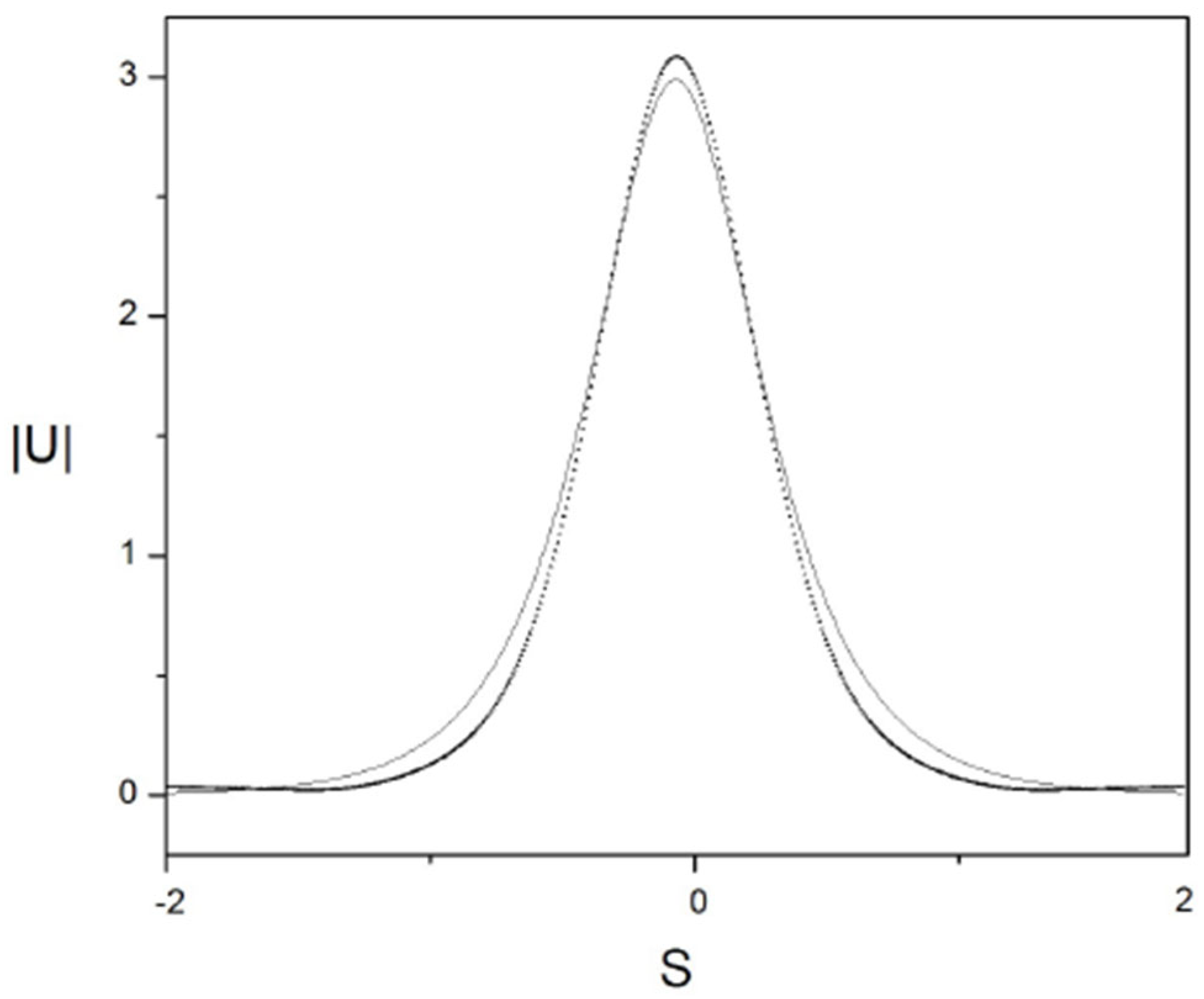
4.1. Variational Results Produced by the Sech Ansatz (16)

We start the analysis by considering the same coefficients of α, β, θ and γ from Equation (32) that were used to generate Figure 1. These coefficients adequately represent a generic case.

First, Figure 2 demonstrates the soliton’s shape as produced by ansatz (16) with parameters obtained from the numerical solution of the Euler–Lagrange Equations (21)–(24), with the initial conditions corresponding to a fixed point of the equations, which are $A=\sqrt{10}$ and $a=7/100$. The respective ansatz is

$$U\left(0,s\right)=\sqrt{10} \mathrm{sech}(100 s/7)$$

(41)

The stationary propagation observed in Figure 2 corroborates that this fixed point is a stable constant solution of Equations (21)–(24).

Next, we take the coefficients

$$\alpha =31.5965, \beta =3.9049, \theta =-13.5328, \gamma =1$$

(42)

in Equation (7) and the initial parameters in ansatz (16), corresponding to the following input:

$$U\left(0,s\right)=4\mathrm{sech}\left(8s\right),$$

(43)

cf. Equation (41). The amplitude and width of expression (43) do not correspond to a fixed point of Equations (22) and (24), hence the solutions of the Euler–Lagrange Equations (21)–(24) produce the solutions shown in Figure 3 and Figure 4. It is a breather, i.e., a solitary wave whose amplitude and width exhibit periodic oscillations along the ζ-axis with the period $\lambda \approx 0.123$.

Another relevant example of breathers is produced by Equations (21)–(24) with the following parameter set, which differs from (42) by a smaller value of coefficient $\beta$ in front of the cubic term,

$$\alpha =31.5965, \beta =1.0149, \theta =-13.5328, \gamma =1,$$

(44)

and initial values of the variational parameters corresponding to the following input:

$$U\left(0,s\right)=4\mathrm{sech}\left(6s\right),$$

(45)

cf. Equation (43). Similar to the examples displayed in Figure 3 and Figure 4, the amplitude and width of expression (45) do not correspond to a fixed point of Equations (22) and (24). In this case, the solution of the Euler–Lagrange Equations (21)–(24) produces the results presented in Figure 5 and Figure 6. They exhibit oscillations of the breather with the period $\lambda \approx 0.411$, which is larger by a factor $\simeq 3.34$ than in Figure 3 and Figure 4.

Lastly, Figure 7 and Figure 8 demonstrate examples of a robust breather featuring much slower oscillations with the period $\lambda \approx 1.888$, which is larger by a factor $\simeq 4.6$ than in Figure 5 and Figure 6. This solution of Equations (21)–(24) was obtained for the following parameter set:

$$\alpha =-6.7658, \beta =14.078, \theta =-13.5153, \gamma =1$$

(46)

and the same initial input (41) as used above, which, in this case, does not represent a fixed point of Equations (22) and (24).

Thus, depending on the values of coefficients $\alpha$, $\beta$ and $\theta$ in Equation (7) and the form of the initial condition, the VA predicts breathers with very different oscillation periods. The values of the coefficients $\alpha$, $\beta$ and $\theta$ used to obtain the solutions shown in Figure 2, Figure 3, Figure 4, Figure 5, Figure 6, Figure 7 and Figure 8 are translated using the material characteristics given [6] into the following values of the physical parameters of the photorefractive crystal:

$$\begin{gathered} x_0=20 \mathsf{\mu }\mathrm{m}\hspace{1em}{k}_0=\frac{2\pi }{{\lambda }_0}=\frac{2\pi }{405}{ \mathrm{n}\mathrm{m}}^{-1} \\ {n}_e=2.2\hspace{1em}{r}_{ef}=30\times {10}^{-12} \mathrm{m}/\mathrm{V} \\ {\lambda }_c=0.5\hspace{1em}\tau =3.3829\times {10}^{-5 }\mathrm{m}/\mathrm{V} \end{gathered}$$

(47)

4.2. Variational Results Produced by the $\sqrt{sech}$ Ansatz (33)

Next, we produce VA predictions based on an alternative analytically tractable ansatz (33) with the evolution of the variational parameters governed by Euler–Lagrange Equations (36)–(39). To begin with, as shown in Figure 9, we produce a stationary soliton generated by initial values of the variational parameters corresponding to the input as follows:

$$U\left(0,s\right)=\sqrt{10 \mathrm{s}\mathrm{e}\mathrm{c}\mathrm{h}\left(13.11 s\right)}$$

(48)

where the amplitude and width correspond to a fixed point of Equations (37) and (39). The respective set of coefficients in Equation (7) are:

$$\alpha =-6.7658, \beta =7.7976, \gamma =1, \theta =-13.5153$$

(49)

Next, to produce a breather (as shown in Figure 10 and Figure 11), we use the same input as (48) but with different coefficients in Equations (7) and (36)–(39), as follows:

$$\alpha =-6.7658, \beta =7.2976, \theta =-13.5153, \gamma =1$$

(50)

In this case, the parameters of the input in (48) do not correspond to a fixed point of Equations (37) and (39); consequently, the simulations of variational Equations (36)–(39) produce a breather with a period of stable oscillations of $\mathsf{\lambda }\approx 0.24$.

Further, the same input as (47) and the same set of coefficients as (49), but with a smaller value of the coefficient in front of the cubic term of $\beta =6.6$ (in this case, the input does not represent a fixed point of Equations (37) and (39), produce the breather shown in Figure 12 and Figure 13. Its oscillation period, $\lambda \approx 0.56$, is larger by a factor $\approx 2.3$ than in Figure 10 and Figure 11.

Lastly, a stable breather with a very large oscillation period of $\lambda \approx 5.8$, which is $\approx$24 times larger than in Figure 12 and Figure 13, is predicted by a VA based on the input

$$U\left(0,s\right)=\sqrt{10\mathrm{s}\mathrm{e}\mathrm{c}\mathrm{h}\left(22.38 s\right)}$$

(51)

for the following coefficients:

$$\alpha =-6.7658, \beta =1.1976, \theta =-13.5153, \gamma =1$$

(52)

in Equations (36)–(39). This slowly oscillating breather (once again initiated by an input that does not correspond to the fixed point of Equations (37) and (39)) is displayed in Figure 14 and Figure 15.

The values of the coefficients $\alpha$, $\beta$ and $\theta$ used to obtain the solutions shown in Figure 9, Figure 10, Figure 11, Figure 12, Figure 13, Figure 14 and Figure 15 are translated using the material characteristics given in [18] into the values of the physical parameters of the photorefractive crystal given in Equation (47), along with $E_p=-2 \mathrm{k}\mathrm{V}/\mathrm{c}\mathrm{m}$ and $E_0=-3.99518\mathrm{k}\mathrm{V}/\mathrm{c}\mathrm{m}$.

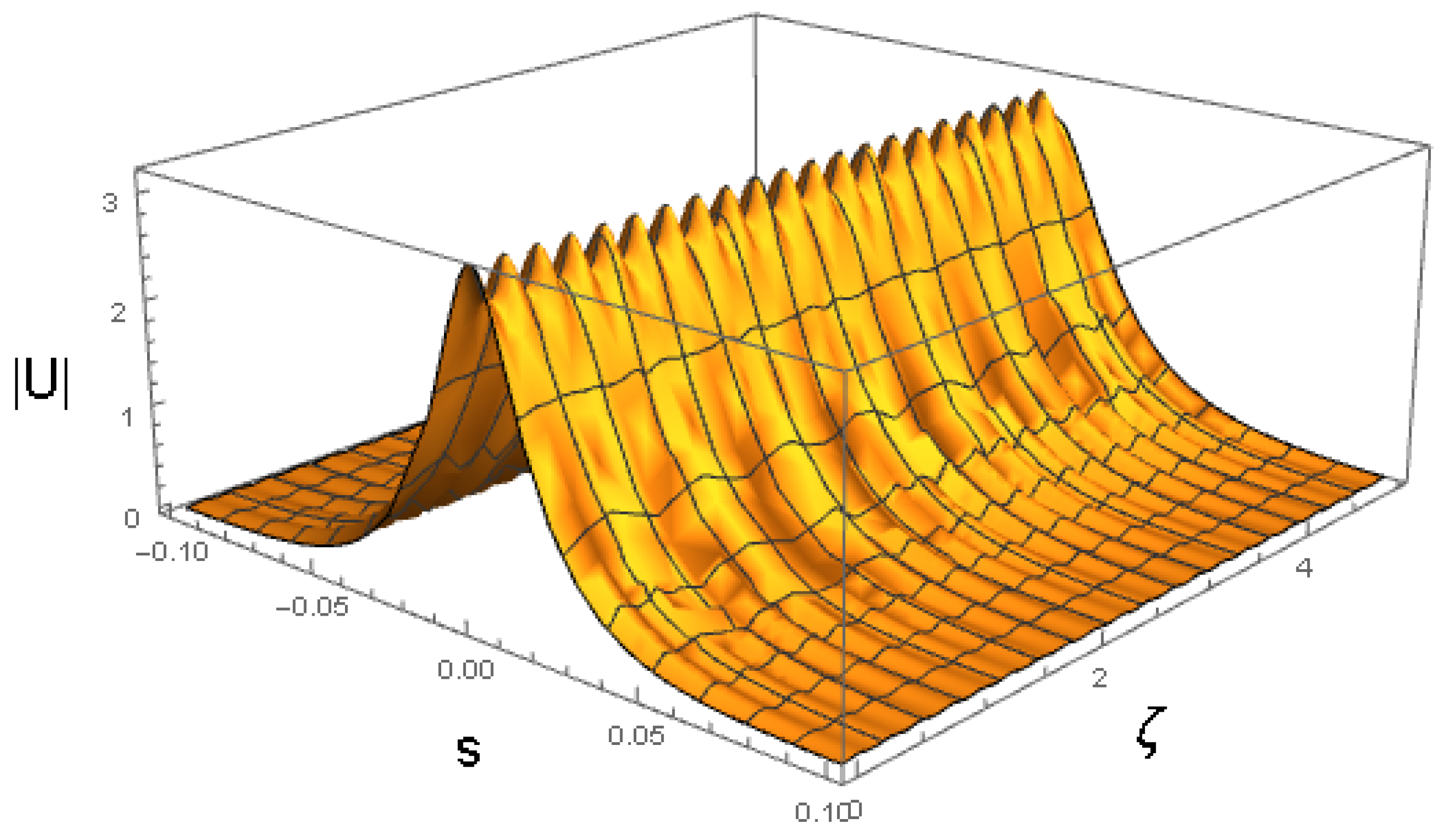
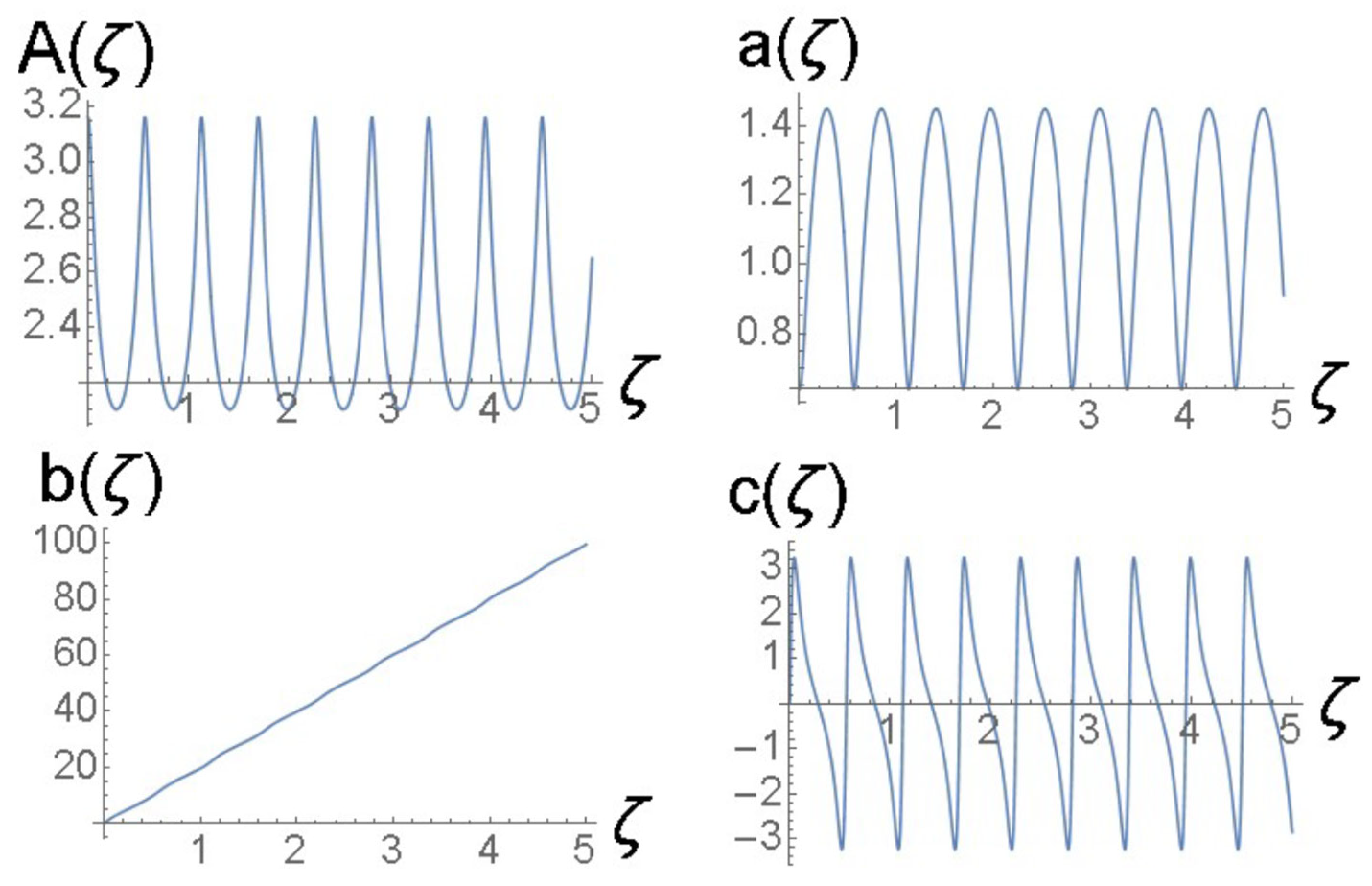
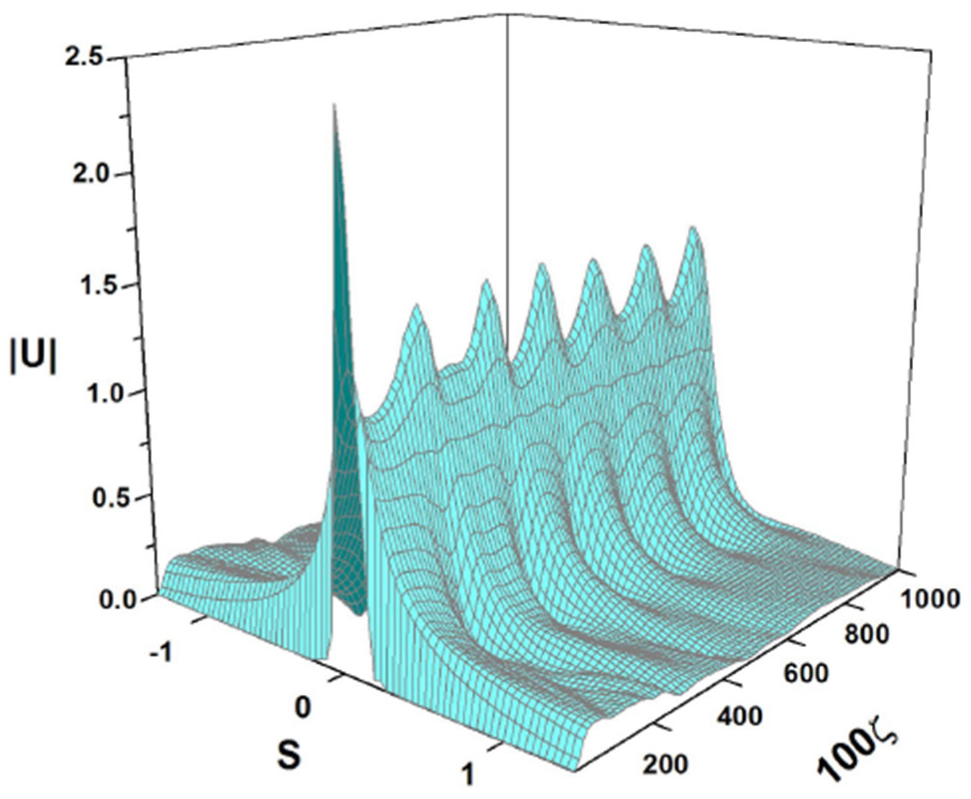
4.3. Direct Simulations of the Evolution of Solitons and Breathers

The predictions of the VA reported above can be verified by means of the full numerical solution of Equation (7). These numerical solutions are obtained by using a fourth-order Runge–Kutta algorithm to advance along ζ, approximating the second derivative $U_{ss}$ with finite differences, including first and second neighbors. To begin with, we solve Equation (7) using the same coefficients given in Equation (32) and the initial condition given in Equation (41), which were used to produce the variational solution shown in Figure 2. The corresponding numerical solution of Equation (7) is displayed in Figure 16. The full simulations produce a stable soliton in perfect agreement with the VA prediction.

The surfaces seen in Figure 2 and Figure 16 look quite similar. In order to appreciate to what extent these surfaces are really similar, we show in Figure 17 the form of the profile $\left|U\left(s,\zeta =20\right)\right|$ given by the numerical solution of Equation (7) (black squares) and the profile obtained from the variational solution (the thin continuous line). It can be seen that the agreement between the two solutions is excellent.

Next, in Figure 18 and Figure 19, we show the numerical solutions of Equation (7) that corroborate the existence of robust breathers, which are quite close to those predicted in Figure 3 and Figure 5 for the same parameters and initial conditions. It is noteworthy that the VA-predicted and numerically found oscillation periods are very close.

To appreciate to what extent the variational solution shown in Figure 5 is similar to the direct numerical solution shown in Figure 19, Figure 20 presents the profiles $\left|U\left(s,\zeta =1\right)\right|$ obtained from the variational solution shown Figure 5 (a thin line) and the profile obtained from the direct numerical solution of Equation (7) (black dots). It can be seen that the agreement between both profiles is very good, thus confirming that the variational method indeed produces solutions that are close to the direct numerical solutions of Equation (7).

The breathing solutions shown in Figure 18 and Figure 19 are produced by using initial conditions that are very close to exact breathers. A natural question is what will happen if one uses an input that is not too close to an exact breather. To address this issue, we show the numerical solution of Equation (7) in Figure 21, which is obtained with the input

$$U\left(s,0\right)=2.958 \mathrm{sech}(100s/7)$$

(53)

and the coefficients given in Equation (46). It can be seen that the input evolves into a breather, even though the initial amplitude of the pulse is significantly higher than the breather’s amplitude. This result implies that even if the breather is significantly perturbed (by increasing its amplitude and reducing its width), the pulse returns to the breather’s shape, indicating that this breather is a robust solution.

All the breather solutions produced by the simulations of Equation (7) demonstrate their robustness against decay into small-amplitude radiation waves. Strictly speaking, the emission of radiation (in the form of the slow decay of an excited state of a fundamental soliton [45]) is generated by any equation of the NLS-type (a well-known fact is that an integrable NLS equation with cubic self-focusing gives rise to exact breather solutions in the form of N-solitons, which are produced by the input in the form of a fundamental soliton multiplied by an arbitrary integer such as N = 2, 3, 4, … [46]). Nevertheless, in our simulations the decay presents a very weak effect, which remains virtually invisible.

We can use the numerical solutions of Equation (7) to corroborate that the VK criterion predicts the stability of the soliton solutions of Equation (7). To this end, we look for solitons corresponding to the same set of coefficients $\left\{\alpha , \beta , \gamma \mathrm{a}\mathrm{n}\mathrm{d} \theta \right\}$ as chosen in Equation (49) and four different values of the propagation constant (k = 21.99, 31.42, 62.83 and 100.53). In each case, we compute the integral power P (see Equation (12)), as shown in Figure 22. This figure shows that dependence $P\left(k\right)$ has a positive slope (i.e., $dP/dk>0$), hence the VK criterion indicates that these solitons are stable solutions, which is corroborated by the simulations of Equation (7).

Figure 17, Figure 18 and Figure 19 show that the separation $\lambda$ between the breathers’ peaks changes if we modify the coefficients of Equation (7). It is noteworthy that that the VA present in Figure 3, Figure 5 and Figure 7 predicts similar changes in λ. To evaluate to what extent the VA-predicted changes in λ are similar to those observed in the direct numerical solutions of Equation (7), we calculate how $\lambda$ depends on $\beta$ according to the direct numerical solutions of Equation (7) and, on the other hand, according to the variational Equations (21)–(24). We focus here on the parameter $\beta$ as this is the coefficient associated with the cubic nonlinearity of Equation (7), which is responsible for the creation and propagation of solitons in NLS-like equations.

In Figure 23, we display the form of function $\lambda \left(\beta \right)$ according to the direct numerical solutions of Equation (7) (black squares) and according to the variational Equations (stars). All the results shown in this figure can be obtained using the coefficients $\alpha =31.60$, $\theta =-13.53$ and $\gamma =1$ in Equation (7) and the initial condition defined in Equation (45).

Figure 23 shows that both procedures (performed using the direct numerical solutions of Equation (7) or the variational equations) demonstrate that λ decreases as $\beta$ increases. This behaviour can be understood if we observe that the definition of $\beta$ (below Equation (6)) combined with Equations (4) and (5) imply that $\Delta n$ will increase if $\beta$ increases. If $\Delta n$ (the refractive index change due to the photorefractive effect) increases, the light velocity in the crystal decreases. Consequently, if $∆t$ is the time interval between two successive maxima in the light intensity of a breather, the distance $v∆t$, advanced by light during this time interval, diminishes if the velocity of light $\left(v\right)$ decreases. In other words, $\lambda =v∆t$ will decrease. This is the physical interpretation of Figure 23. It should be mentioned, however, that a change in $\beta$ is not the only possible cause for a change in λ. In particular, it is known that light absorption may also change the value of λ [47].

The numerical solutions of Equation (7) presented in this subsection as well as the variational solutions presented in Section 4.1 and Section 4.2 show that Equation (7) permits the propagation of solitons and breathers. Consequently, a natural question is if there is a criterion that permits one to forecast if a given solitary-wave input will propagate as a soliton or if it will evolve as a breather. In the case of the cubic NLS equation, the integrability of this equation permits one to answer this question. More precisely, if we consider the input in the form $U\left(s,\zeta =0\right)=A \mathrm{s}\mathrm{e}\mathrm{c}\mathrm{h}(s/a)$, the Zakharov–Shabat equations predict the number of solitons that will be generated as the number of bound eigenstates in a linear problem (in a similar way as in the usual quantum mechanical problem with a given potential well). It is well-known [46] that if the parameters of the input satisfy the inequality $Aa<1/2$, the potential well has no bound states and no solitons appear. In the interval $1/2<Aa<3/2,$ the eigenvalue problem has exactly one bound state, hence exactly one soliton appears. However, when $Aa>3/2$, a second bound state appears, which implies the creation of the superposition of two solitons, i.e., precisely the simplest breather. In other words, in the integrable NLS case, the character of the output (i.e., the generation of a soliton or a breather) is determined by the size of the product $Aa$. For a nonintegrable equation such as Equation (7), there are no exact results like that, although the situation remains qualitatively similar: for relatively small values of $Aa$, the input is able to maintain the self-trapping of a single soliton, but for larger values of $Aa$, the input cannot avoid the generation of at least one additional soliton whose interaction with the original soliton builds a breather. It should be mentioned, however, than the determination of precise criteria that may be helpful to predict if a given solitary-wave initial condition for Equation (7) will evolve as a soliton or as a breather is outside the scope of this article.

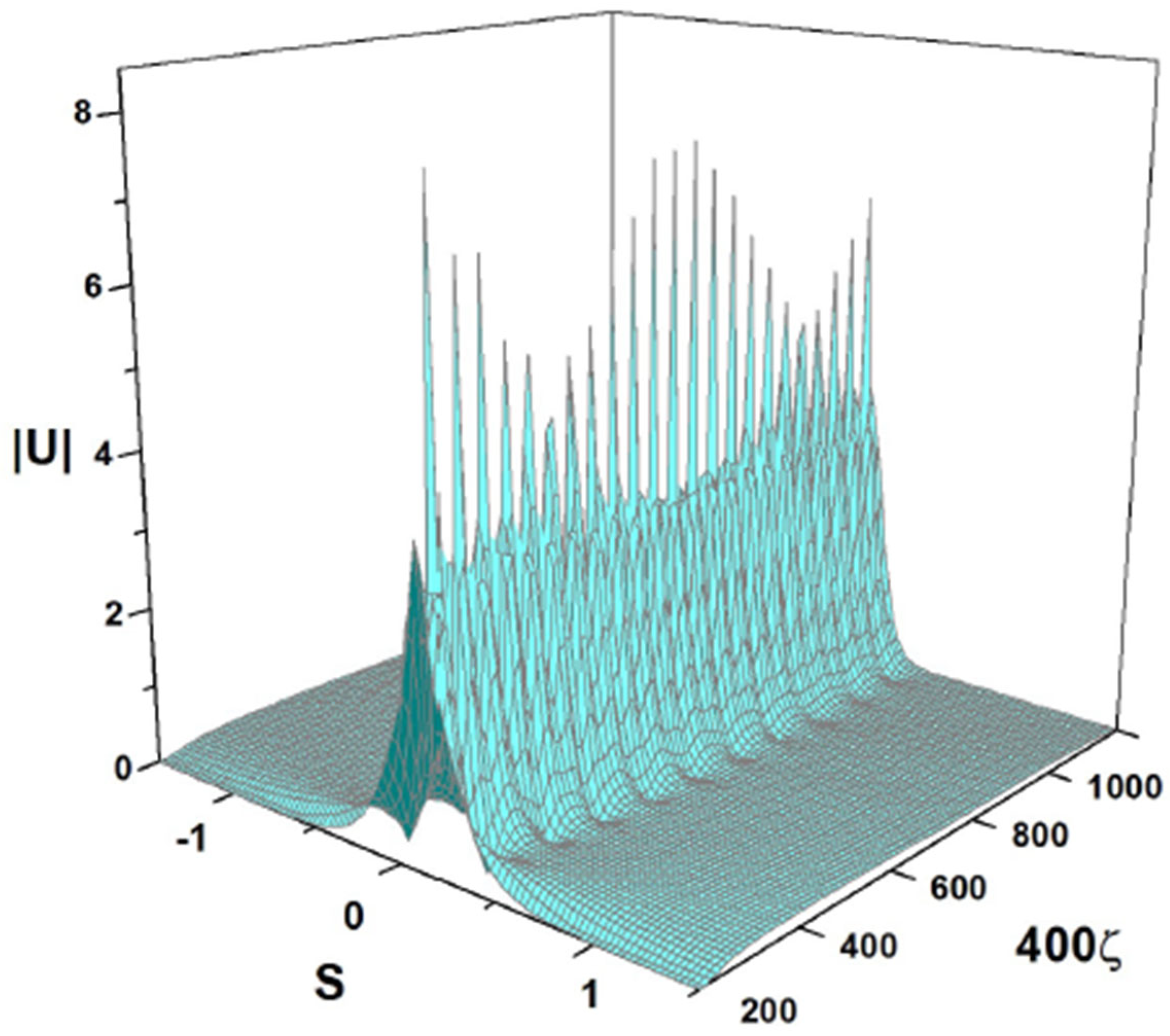
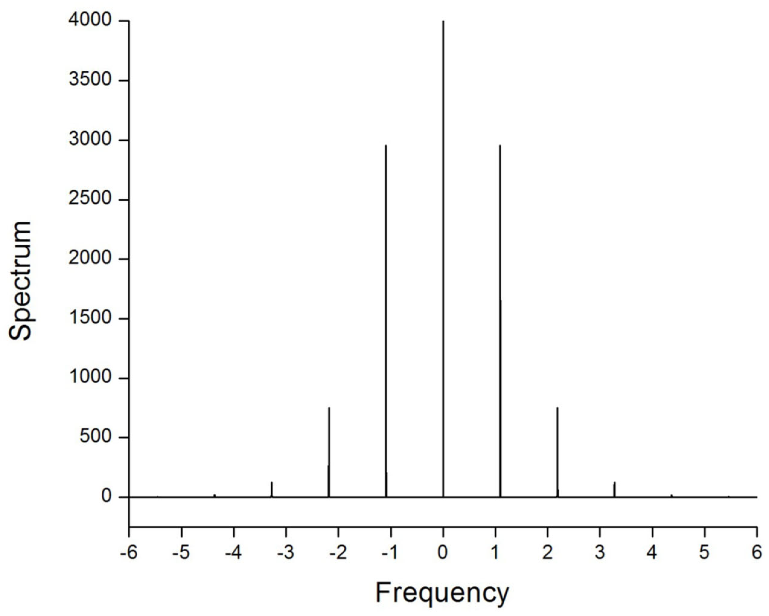
4.4. Breathers Modulated by Beats

The solutions produced by the simulations of Equation (7) in Figure 18, Figure 19 and Figure 21 may be considered as regular breathers as they exhibit strictly periodic oscillations. On the other hand, nonintegrable systems (such as the NLS equation combining the cubic self-defocusing and harmonic-oscillator trapping potential [48]) may give rise, under special conditions, to dynamical states featuring quasi-periodic oscillations. In accordance with this expectation, Equation (7) gives rise, in addition to the regular breathers presented above, to more sophisticated spatially self-trapped modes in the form of breathers featuring long-period beats such as one displayed in Figure 24. It corresponds to coefficients

$$\alpha =-6.7658, \beta =67.6584, \theta =-13.2643, \gamma =1$$

(54)

in Equation (7) and the following input:

$$U\left(s,\zeta =0\right)=\sqrt{10} \mathrm{sech}\left(9.57s\right)$$

(55)

To identify the character of the beats exhibited by the breather displayed in Figure 24, it is relevant to calculate the power spectrum of the oscillations of their amplitude, ${\left|\tilde{U}(\nu )\right|}^2$, where $\tilde{U}(\nu )$ is the Fourier transform of $U(\zeta ,s=0)$ and $\nu$ is the respective spatial frequency.

The power spectrum for the amplitude oscillations of the breather shown in Figure 24 is plotted in Figure 25. In this case, the Fourier transform of $\left|U\left(\zeta ,s=0\right)\right|$ is computed using $2^{14}$ values of this function of $\zeta$, corresponding to 16,384 equally spaced points in the interval of $0\le \zeta \le 7.5$. As ζ is a dimensionless variable, the Fourier transform of $\left|U\left(\zeta ,s=0\right)\right|$ is a function of a dimensionless spatial frequency. It is observed that the discrete spectral components at frequencies $\pm 1.09, \pm 2.19 \mathrm{a}\mathrm{n}\mathrm{d} \pm 3.28$ represent anharmonic oscillations of the breather, while the dc component that concentrates around the zero frequency accounts for long-period beats.

The results presented in this section and in the previous ones show that breathers in photorefractive crystals constitute a subject deserving further investigation. In this connection, it is relevant to mention that the study of breathers in other systems such as linear and nonlinear phononic crystals and granular crystals [49,50,51] as well as the study of discrete breathers [52,53,54] are also interesting fields.

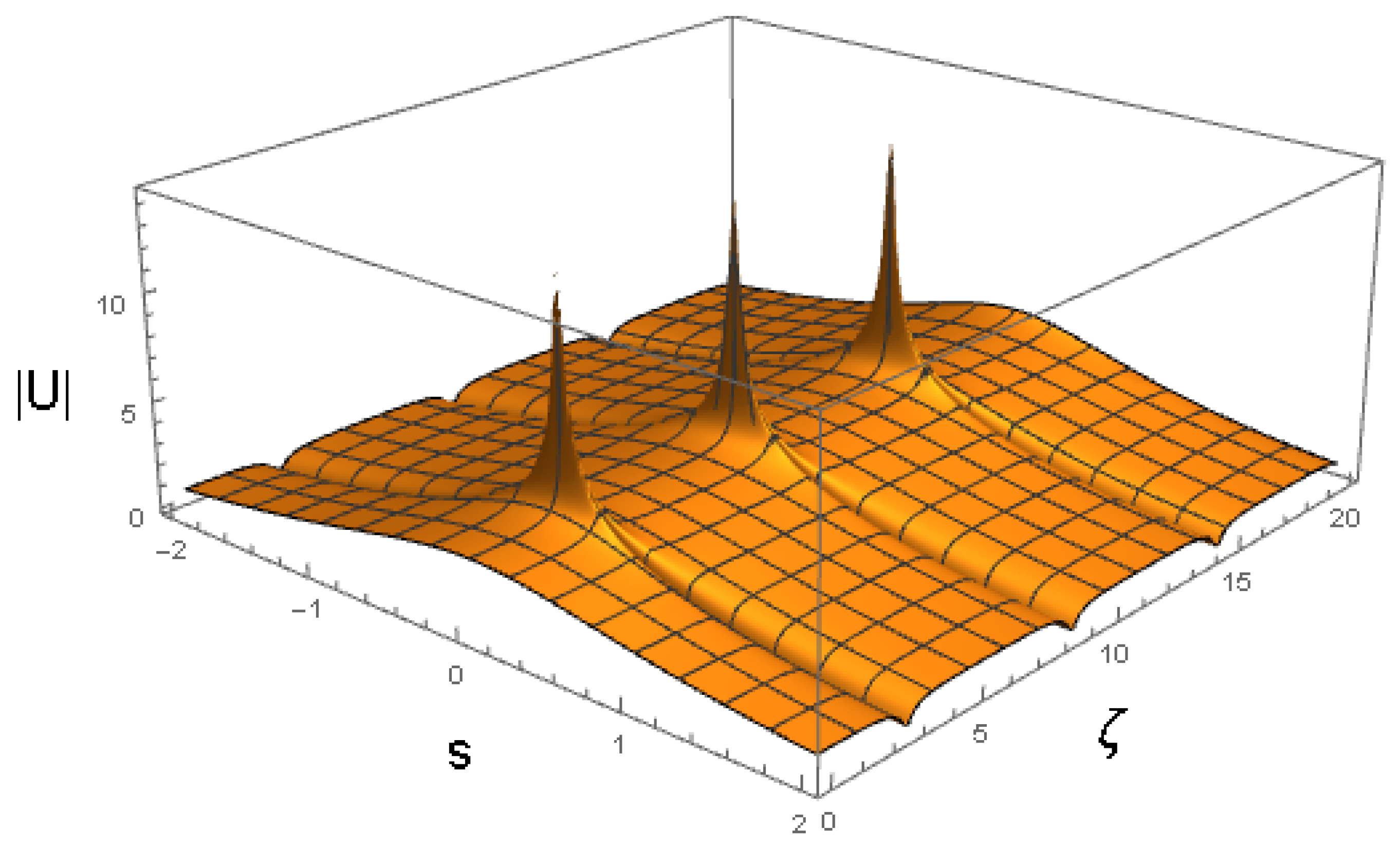
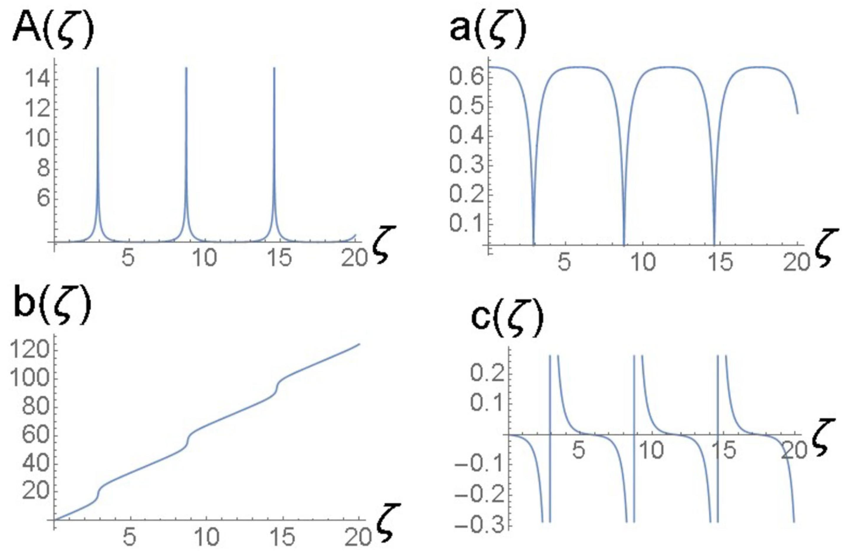
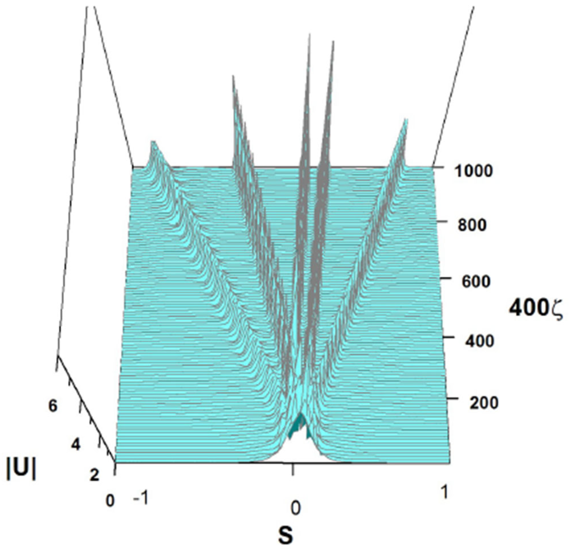
4.5. Splitting Breathers

Another example of a breather with slowly modulated intrinsic oscillations is displayed in Figure 26. It is obtained as a numerical solution of Equation (7) with the same values of coefficients as in Equation (53) and the following input:

$$U\left(s,\zeta =0\right)=\sqrt{10} \mathrm{sech}(8.70 s).$$

(56)

Unlike the dynamical scenarios demonstrated above, this breather splits in two parts: a small solitary wave that moves to the left (towards s < 0) and the principal one, which moves to the right with a small velocity. Although the small solitary wave that moves to the left is not seen in Figure 26 because it is located behind the principal wave, it is visible under the different angle used in Figure 27. Splitting is one of the generic outcomes of the evolution of chirped pulses in equations of the NLS-type [55,56].

Splitting of a single pulse into multiple solitary waves is possible too. A typical example of this type is displayed in Figure 28, where the initial pulse is fragmented into five solitons with weak internal oscillations. In this case, the coefficients of Equation (7) are the same as in Figure 24, i.e., they are given as per Equation (54), and the input is as follows:

$$U\left(s,\zeta =0\right)=\sqrt{10} \mathrm{sech}(4.50 s)$$

(57)

The two examples presented in Figure 27 and Figure 28 show that the solutions of Equation (7) corresponding to localized initial conditions may produce solutions that split into two or more solitary waves. This is not a surprise, as it is well-known that in the case of an integrable NLS equation, a sech input (depending on amplitude $B$ in front of it $\left[U\left(s,\zeta =0\right)=B \mathrm{s}\mathrm{e}\mathrm{c}\mathrm{h}\left(bs\right)\right]$) may generate a soliton or produce a fission into a set of several solitary waves. Without any additional perturbation, the multi-soliton state would form a breather, while any perturbation would split it into a set of separating fundamental solitons. The number of solitons, $N$, is determined by what is usually called the “area” $A$ of the input, i.e., the integral of $U\left(s,\zeta =0\right)$. This integral should not be confused with the norm, which is the integral of ${\left[U\left(s,\zeta =0\right)\right]}^2$, and, unlike the norm, the area is not a dynamical invariant of the NLS equation. In the case of a nonintegrable equation such as Equation (7), there is no exact criterion to predict the number of solitary waves generated by the splitting of the input. However, a qualitative similarity still holds: in the case of Equation (7) the number of fundamental solitons created by the splitting of a sech input increases as the area $A$ of the input increases. We can observe that the value $A_{57}=2.21$ corresponding to the input of (57) is nearly twice as large in comparison to $A_{56}=1.14$ for the pulse of (56), and, as a consequence, the number of waves generated by the splitting increases from 2 to 5. It is interesting to observe that in the integrable case, if an initial pulse with area $A$ splits into two solitary waves, a broader pulse with area $2A$ would split into $2\times 2=4$ new waves. Therefore, the splitting of the pulse of (57) into five new waves (instead of four) is an interesting manifestation of the nonintegrability of Equation (7). On the other hand, an essential similarity with the integrable case is that the initial pulse in (57) splits into a set of solitary waves with unequal amplitudes. Therefore, the fission of solitary waves in the case of Equation (7) presents some similarities to the results observed in the integrable cubic–NLS case, but the similarity is not exact due to the fact that Equation (7) is not integrable.

5. Conclusions

The results presented in this communication show that solitons and breathers exist in biased photovoltaic pyroelectric photorefractive crystals where the light propagation obeys Equation (7). The application of VA (variational approximation) predicts the existence of breathers with different shapes and oscillation periods. The VK (Vakhitov–Kolokolov) criterion correctly indicates that these solitons are stable solutions. The VA is elaborated on the basis of two different ansätze, which are defined in Equations (16) and (33). In both cases, the averaged Lagrangians given by Equations (18) and (34), respectively, involve the dilogarithm function ${\mathrm{L}\mathrm{i}}_2$. Therefore, we refer to these modes as dilogarithmic breathers. The existence of these VA-predicted breathers is then confirmed by full numerical solutions of Equation (7). The numerical results demonstrate that, in addition to the regular (periodic) breathers such as those shown in Figure 18, Figure 19 and Figure 21, Equation (7) also gives rise to robust breathers exhibiting beats (long-period modulations) in their intrinsic dynamics such as the one shown in Figure 24. The spectrum of oscillations of the beating breathers is nearly discrete, thus confirming that the oscillations are indeed subject to long-period quasi-periodic modulations. Another class of numerical solutions demonstrates the spontaneous splitting of the input pulse into two or several secondary quasi-soliton pulses, as shown in Figure 27 and Figure 28. Systematic simulations of the splitting dynamics is a subject for a separate work, which is currently in progress.

References

1. Ashkin, A.; Boyd, C.D.; Dziedzic, J.M.; Smith, R.G.; Ballman, A.A.; Levinstein, J.J.; Nassau, K. Optically-induced refractive index inhomogeneities in LiNbO3 and LiTaO3. Appl. Phys. Lett. 1966, 9, 72. [Google Scholar] [CrossRef]
2. Seguev, M.; Valley, G.C.; Crosignani, B.; Diporto, P.; Yariv, A. Steady-state spatial screening solitons in photorefractive materials with external applied field. Phys. Rev. Lett. 1994, 73, 3211. [Google Scholar] [CrossRef] [PubMed]
3. Segev, M.; Valley, G.C.; Bashaw, M.C.; Taya, M.; Fejer, M.M. Photovoltaic spatial solitons. J. Opt. Soc. Am. B 1997, 14, 1772. [Google Scholar] [CrossRef]
4. Liu, J.S.; Lu, K.Q. Screening-photovoltaic spatial solitons in biased photovoltaic–photorefractive crystals and their self-deflection. J. Opt. Soc. Am. B 1999, 16, 550. [Google Scholar] [CrossRef]
5. Jiang, Q.; Su, Y.; Ji, X. Pyroelectric photovoltaic spatial solitons in unbiased photorefractive crystals. Phys. Lett. A 2012, 376, 3085. [Google Scholar] [CrossRef]
6. Katti, A.; Yadav, R.A. Spatial solitons in biased photovoltaic photorefractive materials with the pyroelectric effect. Phys. Lett. A 2017, 381, 166. [Google Scholar] [CrossRef]
7. Valley, G.C.; Segev, M.; Crosignani, B.; Yariv, A.; Fejer, M.M.; Bashaw, M.C. Dark and bright photovoltaic spatial solitons. Phys. Rev. A 1994, 50, R4457. [Google Scholar] [CrossRef] [PubMed]
8. Taya, M.; Bashaw, M.C.; Fejer, M.M.; Segev, M.; Valley, G.C. Observation of dark photovoltaic spatial solitons. Phys. Rev. A 1995, 52, 3095. [Google Scholar] [CrossRef] [PubMed]
9. She, W.L.; Xu, C.C.; Guo, B.; Lee, W.K. Formation of photovoltaic bright spatial soliton in photorefractive LiNbO3 crystal by a defocused laser beam induced by a background laser beam. J. Opt. Soc. Am. B 2006, 23, 2121. [Google Scholar] [CrossRef]
10. Fazio, E.; Renzi, F.; Rinaldi, R.; Bertolotti, M.; Chauvet, M.; Ramadan, W.; Petris, A.; Vlad, V.I. Screening-photovoltaic bright solitons in lithium niobate and associated single-mode waveguides. App. Phys. Lett. 2004, 85, 2193. [Google Scholar] [CrossRef]
11. Katti, A. Bright optical spatial solitons in a photovoltaic photorefractive waveguide exhibiting the two photon photorefractive effect. Rev. Mex. Física 2023, 69, 021301. [Google Scholar] [CrossRef]
12. Carretero-González, R.; Promislow, K. Localized breathing oscillations of Bose-Einstein condensates in periodic traps. Phys. Rev. A 2002, 66, 033610. [Google Scholar] [CrossRef]
13. Cuevas, J.; English, L.Q.; Kevrekidis, P.G.; Anderson, M. Discrete breathers in a forced-damped array of coupled pendula: Modeling, computation, and experiment. Phys. Rev. Lett. 2009, 102, 224101. [Google Scholar] [CrossRef] [PubMed]
14. Nikolić, S.N.; Ashour, O.A.; Aleksić, N.B.; Belić, M.R.; Chin, S.A. Breathers, solitons and rogue waves of the quintic nonlinear Schrödinger equation on various backgrounds. Nonlinear Dyn. 2019, 95, 2855. [Google Scholar] [CrossRef]
15. Flach, S.; Gorbach, A.V. Discrete breathers—Advances in theory and applications. Phys. Rep. 2008, 467, 1. [Google Scholar] [CrossRef]
16. Burlak, G.; Chen, Z.; Malomed, B.A. Solitons in PT-symmetric systems with spin–orbit coupling and critical nonlinearity. Commun. Nonlinear Sci. Numer. Simul. 2022, 109, 106282. [Google Scholar] [CrossRef]
17. Konar, S.; Yacheslav, V.; Trofimov, A. Some aspects of optical spatial solitons in photorefractive media and their important applications. Pramana 2015, 85, 975. [Google Scholar] [CrossRef]
18. Katti, A.; Yadav, R.A. Optical Spatial Solitons in Photorefractive Materiales; Springer: Singapore, 2021. [Google Scholar] [CrossRef]
19. Ablowitz, M.J.; Segur, H. Solitons and the Inverse Scattering Transform; SIAM: Philadelphia, PA, USA, 1981. [Google Scholar] [CrossRef]
20. Ablowitz, M.J.; Clarkson, P.A. Solitons, Nonlinear Evolution Equations and Inverse Scattering; Cambridge University Press: Cambridge, UK, 1991. [Google Scholar] [CrossRef]
21. Anderson, D. Variational approach to nonlinear pulse propagation in optical fibers. Phys. Rev. A 1983, 27, 3135. [Google Scholar] [CrossRef]
22. Anderson, D.; Lisak, M.; Reichel, T. Asymptotic propagation properties of pulses in a soliton-based optical-fiber communication system. J. Opt. Soc. Am. B 1988, 5, 207. [Google Scholar] [CrossRef]
23. Malomed, B.A.; Parker, D.F.; Smyth, N.F. Resonant shape oscillations and decay of a soliton in a periodically inhomogeneous nonlinear optical fiber. Phys. Rev. E 1993, 48, 1418. [Google Scholar] [CrossRef] [PubMed]
24. Kath, W.L.; Smyth, N.F. Soliton evolution and radiation loss for the nonlinear Schrödinger equation. Phys. Rev. E 1995, 51, 1484. [Google Scholar] [CrossRef] [PubMed]
25. Doty, S.L.; Haus, J.W.; Oh, Y.; Fork, R.L. Soliton interactions on dual-core fibers. Phys. Rev. E 1995, 51, 709. [Google Scholar] [CrossRef] [PubMed]
26. Paré, C.; Florjanczyk, M. Approximate model of soliton dynamics in all-optical couplers. Phys. Rev. A 1990, 41, 6287. [Google Scholar] [CrossRef] [PubMed]
27. Rusin, R.; Kusdiantara, R.; Susanto, H. Variational approximations of soliton dynamics in the Ablowitz-Musslimani nonlinear Schrödinger equation. Phys. Lett. A 2019, 383, 2039. [Google Scholar] [CrossRef]
28. Fujioka, J.; Espinosa, A. Stability of the bright-type algebraic solitary-wave solutions of two extended versions of the nonlinear Schrödinger equation. J. Phys. Soc. Jpn. 1996, 65, 2440. [Google Scholar] [CrossRef]
29. Fujioka, J.; Espinosa, A. Soliton-like solution of an extended NLS equation existing in resonance with linear dispersive waves. J. Phys. Soc. Jpn. 1997, 66, 2601. [Google Scholar] [CrossRef]
30. Fujioka, J.; Espinosa, A. Radiationless higher-order embedded solitons. J. Phys. Soc. Jpn. 2013, 82, 034007. [Google Scholar] [CrossRef]
31. Velasco-Juan, M.; Fujioka, J. Lagrangian nonlocal nonlinear Schrödinger equations. Chaos Solitons Fractals 2022, 156, 111798. [Google Scholar] [CrossRef]
32. Malomed, B.A. Variational methods in nonlinear fiber optics and related fields. Progr. Optics 2002, 43, 71–193. [Google Scholar] [CrossRef]
33. Malomed, B.A. Multidimensional Solitons; American Institute of Physics Publishing: Melville, NY, USA, 2022. [Google Scholar] [CrossRef]
34. Gunter, P.; Huignard, J.P. (Eds.) Photorefractive Materials and Their Applications I and II; Springer: Berlin/Heidelberg, Germany, 1988. [Google Scholar] [CrossRef]
35. Yeh, P. Photorefractive Nonlinear Optics; Wiley: New York, NY, USA, 1993. [Google Scholar]
36. Su, Y.; Jiang, Q.; Ji, X. Coherent interactions of multi bright spatial solitons in biased photorefractive crystals. Optik 2014, 125, 1231. [Google Scholar] [CrossRef]
37. Gradshteyn, I.S.; Ryzhik, I.M. Table of Integrals, Series, and Products; Academic Press: Amsterdam, The Netherlands, 2007. [Google Scholar] [CrossRef]
38. Petrović, M.S.; Strinić, A.I.; Aleksić, N.B.; Belić, M.R. Rotating solitons supported by a spiral waveguide. Phys. Rev. A 2018, 98, 063822. [Google Scholar] [CrossRef]
39. Kalashnikov, V.L.; Apolonski, A. Energy scalability of mode-locked oscillators: A completely analytical approach to analysis. Opt. Express 2010, 18, 25757. [Google Scholar] [CrossRef] [PubMed]
40. Vakhitov, N.G.; Kolokolov, A.A. Stationary solutions of the wave equation in a medium with nonlinearity saturation. Radiophys. Quantum Electron. 1973, 16, 783. [Google Scholar] [CrossRef]
41. Kolokolov, A.A. Stability of stationary solutions of nonlinear wave equations. Radiophys. Quantum Electron. 1974, 17, 1016. [Google Scholar] [CrossRef]
42. Yang, J. Nonlinear Waves in Integrable and Nonintegrable Systems; SIAM series on Mathematical Modeling and Computation; SIAM: Philadelphia, PA, USA, 2010. [Google Scholar] [CrossRef]
43. Ablowitz, M.J.; Antar, N.; Bakirtaş, I.; Boaz, I. Band-gap boundaries and fundamental solitons in complex two-dimensional nonlinear lattices. Phys. Rev. A 2010, 81, 033834. [Google Scholar] [CrossRef]
44. Abdullaev, F.K.; Gammal, A.; Tomio, L.; Frederico, T. Stability of Trpped Bose-Einstein condensates. Phys. Rev. A 2001, 63, 043604. [Google Scholar] [CrossRef]
45. Kuznetsov, E.A.; Mikhailov, A.V.; Shimokhin, I.A. Nonlinear interaction of solitons and radiation. Physica D 1995, 87, 201–205. [Google Scholar] [CrossRef]
46. Satsuma, J.; Yajima, N.B. Initial Value problems of one-dimensional self-modulation of nonlinear waves in dispersive media. Suppl. Prog. Theor. Phys. 1974, 55, 284. [Google Scholar] [CrossRef]
47. Fazio, E.; Babin, V.; Bertolotti, M.; Vlad, V. Solitonlike propagation in photorefractive crystals with large optical activity and absorption. Phys. Rev. E 2002, 66, 016605. [Google Scholar] [CrossRef]
48. Bland, T.; Parker, N.G.; Proukakis, N.P.; Malomed, B.A. Probing quasi-integrability of the Gross-Pitaevskii equation in a harmonic-oscillator potential. J. Phys. B 2018, 51, 205303. [Google Scholar] [CrossRef]
49. Liu, Z.G.; Zhang, J.; Wang, Y.S.; Huang, G. Analytical solutions of solitary waves and their collision stability in a pre-compressed one-dimensional granular crystal. Nonlinear Dyn. 2021, 104, 4293–4309. [Google Scholar] [CrossRef]
50. Boechler, N.; Theocharis, G.; Job, S.; Kevrekidis, P.G.; Porter, M.A.; Daraio, C. Discrete breathers in one-dimensional diatomic granular crystals. Phys. Rev. Lett. 2010, 104, 244302. [Google Scholar] [CrossRef] [PubMed]
51. Chong, C.; Porter, M.A.; Kevrekidis, P.G.; Daraio, C. Nonlinear coherent structures in granular crystals. J. Phys. Condens. Matter 2017, 29, 413003. [Google Scholar] [CrossRef] [PubMed]
52. Dimitriev, S.V.; Korznikova, E.A.; Baimova, Y.A.; Velarde, M.G. Discrete breathers in crystals. Phys.-Uspekhi 2016, 59, 446. [Google Scholar] [CrossRef]
53. Duran, H.; Cuevas-Maraver, J.; Kevrekidis, P.G.; Vainchtein, A. Discrete breathers in a mechanical metamaterial. Phys. Rev. E 2023, 107, 014220. [Google Scholar] [CrossRef] [PubMed]
54. Ovchinnikov, A.A.; Flach, S. Discrete Breathers in Systems with Homogeneous Potentials: Analytic Solutions. Phys. Rev. Lett. 1999, 83, 248. [Google Scholar] [CrossRef]
55. Kaup, D.J.; El-Reedy, J.; Malomed, B.A. Effect of chirp on soliton production. Phys. Rev. E 1994, 50, 1635. [Google Scholar] [CrossRef] [PubMed]
56. Erkintalo, M.; Hammani, M.K.; Kibler, B.; Finot, C.; Akhmediev, N.; Dudley, J.M.; Genty, G. Higher-order modulation instability in nonlinear fiber optics. Phys. Rev. Lett. 2011, 107, 253901. [Google Scholar] [CrossRef]
Figure 1. Values of the VA-predicted VK derivative d P / d k for the family of stationary solitons based on ansatz (16) as produced by Equation (31) with the coefficients fixed as per Equation (32).
Axioms 13 00338 g001
Figure 2. U ( s , ζ ) as produced by ansatz (16), with the variational parameters obtained from the numerical solution of Equations (21)–(24) with coefficients (32) and an initial condition corresponding to input (41), which represents the fixed point of the equations. The values of coefficients (32) correspond to E p y = 12.7   k V / c m , E 0 = 3.99518   k V / c m , E p = 2   k V / c m and the physical parameters shown in Equation (47). The counterpart of this picture, produced by full simulations of the GNLSE (7), is presented below in Section 4.3.
Axioms 13 00338 g002
Figure 3. The VA-predicted breather for the coefficients chosen as per Equation (42) and the input corresponding to Equation (43). The values of coefficients (42) correspond to E p y = 2.31   k V / c m , E 0 = 4.00035   k V / c m , E p = 9.34   k v / c m and the physical parameters shown in Equation (47). The counterpart of this dynamical picture, produced by full simulations of the GNLSE (7), is presented below in Section 4.3.
Axioms 13 00338 g003
Figure 4. Solutions of the Euler–Lagrange Equations (21)–(24) for variational parameters A ζ ,   a ζ ,   b ζ   a n d   c ζ for the same case as shown in Figure 3.
Axioms 13 00338 g004
Figure 5. The same as in Figure 3, but for the parameters of (44) and an input corresponding to Equation (45). The values of the coefficients (44) correspond to E p y = 0.6   k V / c m , E 0 = 3.99518   k V / c m , E p = 9.34   k V / c m and the other physical parameters shown in Equation (47). The counterpart of this dynamical picture, produced by full simulations of the GNLSE (7), is presented below in Section 4.3.
Axioms 13 00338 g005
Figure 6. Solutions of the Euler–Lagrange Equations (21)–(24) for variational parameters A ζ ,   a ζ ,   b ζ   a n d   c ζ for the same case as shown in Figure 5.
Axioms 13 00338 g006
Figure 7. The same as in Figure 3, but for the parameters of (46) and an input corresponding to Equation (41). The values of coefficients (46) correspond to E p y = 8.32   k V / c m , E 0 = 3.99518   k V / c m , E p = 2   k V / c m and the other physical parameters shown in Equation (47).
Axioms 13 00338 g007
Figure 8. Solutions of the Euler–Lagrange Equations (21)–(24) for the variational parameters A ζ ,   a ζ ,   b ζ a n d   c ζ for the same case as shown in Figure 7.
Axioms 13 00338 g008
Figure 9. Soliton obtained with ansatz (33). In this case, the variational parameters evolve according to the Euler–Lagrange Equations (36)–(39) with the coefficients shown in Equation (49) and the initial condition given in Equation (48). The values of the coefficients in (49) correspond to E p y = 4.61   k V / c m , E p = 2   k V / c m , E 0 = 3.99518   k V / c m and the physical parameters shown in Equation (47).
Axioms 13 00338 g009
Figure 10. VA-predicted breather obtained with the ansatz (33). It is plotted with the variational parameters evolving according to Euler–Lagrange Equations (36)–(39) with the coefficients chosen as per Equation (50) and the initial condition corresponding to Equation (48). The values of the coefficients of (50) correspond to E p y = 4.31   k V / c m , E p = 2   k V / c m , E 0 = 3.99518   k V / c m and the other physical parameters shown in Equation (47).
Axioms 13 00338 g010
Figure 11. Solutions of the Euler–Lagrange Equations (36)–(39) for the variational parameters A ζ ,   a ζ ,   b ζ   a n d   c ζ , for the same case as shown in Figure 10.
Axioms 13 00338 g011
Figure 12. The same as in Figure 10, except β = 6.6 . This value, and coefficients α , θ and γ given in Equation (50), correspond to E p y = 3.9   k V / c m , E p = 2   k V / c m , E 0 = 3.99518 k V / c m and the other physical parameters shown in Equation (47).
Axioms 13 00338 g012
Figure 13. Solutions of the Euler–Lagrange Equations (36)–(39) for the variational parameters A ζ ,   a ζ ,   b ζ   a n d c ζ , for the same case as shown in Figure 12.
Axioms 13 00338 g013
Figure 14. Breather produced by ansatz (33). In this case, the variational parameters evolve according to the Euler–Lagrange Equations (36)–(39) along with the coefficients shown in Equation (52) and the initial condition given in Equation (51). The values of the coefficients in (52) correspond to E p y = 0.71   k V / c m , E p = 2   k V / c m , E 0 = 3.99518 k V / c m and the other physical parameters shown in Equation (47).
Axioms 13 00338 g014
Figure 15. Solutions of the Euler–Lagrange Equations (36)–(39) for the variational parameters A ζ ,   a ζ ,   b ζ   a n d   c ζ , for the same case as shown in Figure 14.
Axioms 13 00338 g015
Figure 16. Results of the numerical simulations of Equation (7) with the same coefficients as in Equation (32) and the same input as in Equation (41), which were used above to produce the VA solution displayed in Figure 2.
Axioms 13 00338 g016
Figure 17. Profiles | U s , ζ = 20 | obtained from the numerical solution of Equation (7) shown in Figure 16 (black squares) and the variational solution shown in Figure 2 (the thin line).
Axioms 13 00338 g017
Figure 18. Results of the numerical simulations of Equation (7) with the same coefficients as Equation (42) and the same input as Equation (43), which were used above to produce the VA solution displayed in Figure 3.
Axioms 13 00338 g018
Figure 19. Results of the numerical simulations of Equation (7) with the same coefficients as Equation (44) and the same input as Equation (45), which were used above to produce the VA solution displayed in Figure 5.
Axioms 13 00338 g019
Figure 20. Profiles | U s , ζ = 1 | obtained from the numerical solution of Equation (7) shown in Figure 19 (black dots) and the variational solution shown in Figure 5 (thin line).
Axioms 13 00338 g020
Figure 21. Numerical solution of Equation (7) for the coefficients shown in (46) and the initial condition in (53).
Axioms 13 00338 g021
Figure 22. Optical power P vs. the propagation constant k of the soliton solutions of Equation (7) with the coefficients given in Equation (49).
Axioms 13 00338 g022
Figure 23. Separation λ between the breather’s peaks as a function of β . Black squares represent direct numerical solutions of Equation (7) and stars represent the variational solution using the ansatz (16). The input is taken as per Equation (45) and the other coefficients in Equation (7) are α = 31.60 , θ = 13.53 and γ = 1 .
Axioms 13 00338 g023
Figure 24. Beating breather, obtained as a numerical solution of Equation (7) with the parameters of (54) and the input of (55). The values of the coefficients of (54) correspond to the physical parameters given in Equation (47): E p y = 40   k V / c m , E 0 = 3.92098   k V / c m and E p = 2 k V / c m .
Axioms 13 00338 g024
Figure 25. The power spectrum of the amplitude function U ( ζ , s = 0 ) corresponding to the breather shown in Figure 24.
Axioms 13 00338 g025
Figure 26. Numerical solution of Equation (7) with values of the parameters of (54) and the input of (56). These coefficients correspond to the physical parameters shown in Equation (47), where E p y = 40   k V / c m , E 0 = 3.92098   k V / c m and E p = 2   k V / c m .
Axioms 13 00338 g026
Figure 27. The same as in Figure 26, but observed from a different direction.
Axioms 13 00338 g027
Figure 28. Splitting of the input pulse into five secondary ones, exhibited by the numerical solution of Equation (7) with the coefficients shown in Equation (54) and the initial condition of (57). These coefficients correspond to the physical parameters given in Equation (47), where E p y = 40   k V / c m , E 0 = 3.92098   k V / c m and E p = 2   k V / c m .
Axioms 13 00338 g028
Disclaimer/Publisher’s Note: The statements, opinions and data contained in all publications are solely those of the individual author(s) and contributor(s) and not of MDPI and/or the editor(s). MDPI and/or the editor(s) disclaim responsibility for any injury to people or property resulting from any ideas, methods, instructions or products referred to in the content.