On Certain Properties of Parametric Kinds of Apostol-Type Frobenius–Euler–Fibonacci Polynomials

Abstract

This paper presents an overview of cosine and sine Apostol-type Frobenius–Euler–Fibonacci polynomials, as well as several identities that are associated with these polynomials. By applying a partial derivative operator to the generating functions, the authors obtain derivative formulae and finite combinatorial sums involving these polynomials and numbers. Additionally, the paper establishes connections between cosine and sine Apostol-type Frobenius–Euler–Fibonacci polynomials of order $\alpha$ and several other polynomial sequences, such as the Apostol-type Bernoulli–Fibonacci polynomials, the Apostol-type Euler–Fibonacci polynomials, the Apostol-type Genocchi–Fibonacci polynomials, and the Stirling–Fibonacci numbers of the second kind. The authors also provide computational formulae and graphical representations of these polynomials using the Mathematica program.

1. Introduction

Formal research on special polynomials and their associated special numbers has been conducted by numerous scholars. Specifically, the generating functions of these polynomials have been utilized to derive various identities, sum formulae, and symmetric formulae containing these polynomials. Recently, several researchers [1,2,3,4,5] have developed generating functions for new families of special polynomials, including Hermite, Bernoulli, Euler, and Genocchi polynomials. These authors have established the fundamental properties of these polynomials and derived a variety of identities and relationships between trigonometric functions and two parametric kinds of special polynomials using generating functions. The partial derivative operator has been employed to obtain derivative formulae and finite combinatorial sums that involve the mentioned polynomials and numbers. Additionally, these special polynomials facilitate the straightforward derivation of several important identities.

For any $u\in \mathbb{C}$, $u\ne 1$ and $\xi \in \mathbb{R}$, the Apostol-type Frobenius–Euler polynomials ${\mathbb{H}}_w^{\left(\alpha \right)}(\xi ;u;\lambda )$ of order $\alpha \in \mathbb{C}$ are defined (see [3,6,7,8]) as follows:

$${\left(\frac{1-u}{\lambda e^d-u}\right)}^{\alpha }{e}^{\xi d}=\sum _{w=0}^{\infty }{\mathbb{H}}_w^{\left(\alpha \right)}(\xi ;u;\lambda )\frac{d^w}{w!},\mid d\mid <\mid \ln \left(\frac{\lambda }{u}\right)\mid .$$

(1)

For $\xi =0$, ${\mathbb{H}}_w^{\left(\alpha \right)}(u;\lambda )={\mathbb{H}}_w^{\left(\alpha \right)}(0;u;\lambda )$ are called the Apostol-type Frobenius–Euler numbers of order $\alpha$. From (1), we see that

$${\mathbb{H}}_w^{\left(\alpha \right)}(\xi ;u;\lambda )=\sum _{s=0}^w\left({\displaystyle \genfrac{}{}{0pt}{}{w}{s}}\right){\mathbb{H}}_s^{\left(\alpha \right)}(u;\lambda ){\xi }^{w-s},$$

(2)

and

$${\mathbb{H}}_w^{\left(\alpha \right)}(\xi ;-1;\lambda )={\mathbb{E}}_w^{\left(\alpha \right)}(\xi ;\lambda ),$$

(3)

where ${\mathbb{E}}_w^{\left(\alpha \right)}(\xi ;\lambda )$ are the wth Apostol–Euler polynomials of order $\alpha$.

The generalized $\lambda$-Stirling numbers of the second kind $S(w,s;\lambda )$ are provided by (see [9])

$$\frac{{(\lambda e^d-1)}^s}{s!}=\sum _{w=0}^{\infty }S(w,s;\lambda )\frac{d^w}{w!},$$

(4)

for $\lambda \in \mathbb{C}$ and $s\in \mathbb{N}=\{0,1,2,\cdots ,\}$, where $\lambda =1$ yields the usual Stirling numbers of the second kind given by (see [4,10])

$$\frac{{(e^d-1)}^s}{s!}=\sum _{w=0}^{\infty }S(w,s)\frac{d^w}{w!}.$$

(5)

With reference to (4), the $\lambda$-array type polynomials $S(w,s;\xi ;\lambda )$ are given by (see [11])

$$\frac{{(\lambda e^d-1)}^s}{s!}{e}^{\xi d}=\sum _{w=0}^{\infty }S(w,s;\xi ;\lambda )\frac{d^w}{w!}.$$

(6)

The Apostol-type Bernoulli polynomials ${\mathbb{B}}_w^{\left(\alpha \right)}(\xi ;\lambda )$ of order $\alpha$, the Apostol-type Euler polynomials ${\mathbb{E}}_w^{\left(\alpha \right)}(\xi ;\lambda )$ of order $\alpha$, and the Apostol-type Genocchi polynomials ${\mathbb{G}}_w^{\left(\alpha \right)}(\xi ;\lambda )$ of order $\alpha$ are introduced by (see [5,9])

$${\left(\frac{d}{\lambda e^d-1}\right)}^{\alpha }{e}^{\xi d}=\sum _{w=0}^{\infty }{\mathbb{B}}_w^{\left(\alpha \right)}(\xi ;\lambda )\frac{d^w}{w!}\left(\mid d+\log \lambda \mid <2\pi \right),$$

(7)

$${\left(\frac{2}{\lambda e^d+1}\right)}^{\alpha }{e}^{\xi d}=\sum _{w=0}^{\infty }{\mathbb{E}}_w^{\left(\alpha \right)}(\xi ;\lambda )\frac{d^w}{w!}\left(\mid d+\log \lambda \mid <\pi \right),$$

(8)

and

$${\left(\frac{2d}{\lambda e^d+1}\right)}^{\alpha }{e}^{\xi d}=\sum _{w=0}^{\infty }{\mathbb{G}}_w^{\left(\alpha \right)}(\xi ;\lambda )\frac{d^w}{w!},\left(\mid d+\log \lambda \mid <\pi \right),$$

(9)

respectively.

Obviously, we have

$${\mathbb{B}}_w^{\left(\alpha \right)}\left(\lambda \right)={\mathbb{B}}_w^{\left(\alpha \right)}(0;\lambda ),{\mathbb{E}}_w^{\left(\alpha \right)}\left(\lambda \right)={\mathbb{E}}_w^{\left(\alpha \right)}(0;\lambda ),{\mathbb{G}}_w^{\left(\alpha \right)}\left(\lambda \right)={\mathbb{G}}_w^{\left(\alpha \right)}(0;\lambda ).$$

The field of Golden calculus, also known as F-calculus, traces its origins back to the nineteenth century, when its diverse applications in areas like mathematics, physics, and engineering came to light. The concepts and notation used in Golden calculus are derived from various sources [12,13,14,15].

The Fibonacci sequence is introduced as follows:

$$F_w=F_{w-1}+F_{w-2},w\ge 2$$

where $F_0=0$, $F_1=1$. Fibonacci numbers can be written explicitly in terms of

$$F_w=\frac{{\varphi }^w-{\psi }^w}{\varphi -\psi },$$

where $\varphi =\frac{1+\sqrt{5}}{2}$ and $\psi =\frac{1-\sqrt{5}}{2}$; $\varphi \approx 1.6180339\cdots$ is called the Golden ratio. In many different disciplines of science and mathematics, the Golden ratio is a number that occurs frequently. The various properties of the Golden ratio have been extensively studied by Pashaev and Nalci [14]. Other references include Pashaev [15], Krot [16], and Pashaev and Ozvatan [17].

The definition of F-factorial is

$$F_1{F}_2{F}_3\cdots F_w=F_w!,$$

(10)

where $F_0!=1$. The binomial theorem for the F-analogues, also known as the Golden binomial theorem, is expressed as

$${(\xi +\nu )}^w:={(\xi +\nu )}_F^w=\sum _{l=0}^w{\left({\displaystyle \genfrac{}{}{0pt}{}{w}{l}}\right)}_F{(-1)}^{\left(\genfrac{}{}{0pt}{}{l}{2}\right)}{\xi }^{w-l}{\nu }^l,$$

(11)

using Golden binomial coefficients, known as Fibonomials

$${\left(\genfrac{}{}{0pt}{}{w}{l}\right)}_F=\frac{F_w!}{F_{w-l!}{F}_l!},$$

with w and l being nonnegative integers, $w\ge l$. The Fibonomial coefficients have the following identity:

$${\left(\genfrac{}{}{0pt}{}{w}{l}\right)}_F{\left(\genfrac{}{}{0pt}{}{l}{m}\right)}_F={\left(\genfrac{}{}{0pt}{}{w}{m}\right)}_F{\left(\genfrac{}{}{0pt}{}{w-m}{l-m}\right)}_F.$$

(12)

The F-derivative is introduced as follows:

$$\frac{{\partial }_F}{{\partial }_F\xi }\left(f\left(\xi \right)\right)=\frac{f\left(\varphi \xi \right)-f(-\frac{\xi }{\varphi })}{(\varphi -(-\frac{1}{\varphi }))\xi }.$$

(13)

The Golden exponential functions of the first and second variety are

$$e_F\left(\xi \right)=\sum _{w=0}^{\infty }\frac{{\left(\xi \right)}_F^w}{F_w!}$$

(14)

and

$$E_F\left(\xi \right)=\sum _{w=0}^{\infty }{(-1)}^{\left(\genfrac{}{}{0pt}{}{w}{2}\right)}\frac{{\left(\xi \right)}_F^w}{F_w!},$$

(15)

where

$${(\xi +\nu )}^w:={(\xi +\nu )}_F^w=\sum _{l=0}^w{\left({\displaystyle \genfrac{}{}{0pt}{}{w}{l}}\right)}_F{(-1)}^{\left(\genfrac{}{}{0pt}{}{l}{2}\right)}{\xi }^{w-l}{\nu }^l.$$

(16)

Shortly, we use the following notations throughout the paper:

$$e_F\left(\xi \right)=\sum _{w=0}^{\infty }\frac{{\xi }^w}{F_w!}$$

and

$$E_F\left(\xi \right)=\sum _{w=0}^{\infty }{(-1)}^{\left(\genfrac{}{}{0pt}{}{w}{2}\right)}\frac{{\xi }^w}{F_w!},$$

respectively.

The expressions $e_F\left(\xi \right)$ and $E_F\left(\xi \right)$ satisfy the following identity (see [13]):

$$e_F^{\xi }{E}_F^{\nu }=e_F^{{(\xi +\nu )}_F}.$$

(17)

The Apostol-type Bernoulli–Fibonacci polynomials ${\mathbb{B}}_{w,F}^{\left(\alpha \right)}(\xi ;\lambda )$ of order $\alpha$, the Apostol-type Euler–Fibonacci polynomials ${\mathbb{E}}_{w,F}^{\left(\alpha \right)}(\xi ;\lambda )$ of order $\alpha$, and the Apostol-type Genocchi–Fibonacci polynomials ${\mathbb{G}}_{w,F}^{\left(\alpha \right)}(\xi ;\lambda )$ of order $\alpha$ are defined by (see [18,19,20]):

$${\left(\frac{d}{\lambda e_F^d-1}\right)}^{\alpha }{e}_F^{\xi d}=\sum _{w=0}^{\infty }{\mathbb{B}}_{w,F}^{\left(\alpha \right)}(\xi ;\lambda )\frac{d^w}{F_w!},$$

(18)

$${\left(\frac{2}{\lambda e_F^d+1}\right)}^{\alpha }{e}_F^{\xi d}=\sum _{w=0}^{\infty }{\mathbb{E}}_{w,F}^{\left(\alpha \right)}(\xi ;\lambda )\frac{d^w}{F_w!},$$

(19)

and

$${\left(\frac{2d}{\lambda e_F^d+1}\right)}^{\alpha }{e}_F^{\xi d}=\sum _{w=0}^{\infty }{\mathbb{G}}_{w,F}^{\left(\alpha \right)}(\xi ;\lambda )\frac{d^w}{F_w!},$$

(20)

respectively.

Clearly, we have

$${\mathbb{B}}_{w,F}^{\left(\alpha \right)}\left(\lambda \right)={\mathbb{B}}_{w,F}^{\left(\alpha \right)}(0;\lambda ),{\mathbb{E}}_{w,F}^{\left(\alpha \right)}\left(\lambda \right)={\mathbb{E}}_{w,F}^{\left(\alpha \right)}(0;\lambda ),{\mathbb{G}}_{w,F}^{\left(\alpha \right)}\left(\lambda \right)={\mathbb{G}}_{w,F}^{\left(\alpha \right)}(0;\lambda ).$$

In [19], Kızılateş and Öztürk defined two parametric types of the Apostol Bernoulli–Fibonacci polynomials, the Apostol Euler–Fibonacci polynomials, and the Apostol Genocchi–Fibonacci polynomials of order $\alpha$ and obtained some properties for these type of polynomials using Golden calculus. In [21], the authors introduced the generalized Apostol-type Frobenius–Euler–Fibonacci polynomials and numbers using (14) and (15). With this definition, the authors defined Frobenius–Euler–Fibonacci polynomials of the Apostol type in two variables, but in this paper, we give a different generalization of these polynomials.

Given the aforementioned studies, we propose a new class of two-variable polynomials, which includes those defined by Equation (1) through the application of Golden calculus. We introduce the use of generating functions to define parametric Apostol-type Frobenius–Euler–Fibonacci polynomials using the principles of Golden calculus. By employing the associated generating functions and functional equations, we establish numerous properties for these particular polynomials. We present several properties of this polynomial family, such as recurrence relations, summation formulae, and derivative relations, by utilizing their generating function and functional equation. Furthermore, we establish connections between parametric kinds of the Apostol-type Frobenius–Euler–Fibonacci polynomials of order $\alpha$ and various other polynomial sequences, including the Apostol-type Bernoulli–Fibonacci polynomials, the Apostol-type Euler–Fibonacci polynomials, the Apostol-type Genocchi–Fibonacci polynomials, and the Stirling–Fibonacci numbers of the second kind. Finally, we give zeros and graphical illustrations for the parametric kinds of Apostol-type Frobenius–Euler–Fibonacci polynomials.

2. Two Parametric Kinds of Apostol-Type Frobenius–Euler–Fibonacci Polynomials

According to Krot’s definition [16], the Fibonomial convolution of two sequences involves the following: Let $a_n$ and $b_n$ be two sequences with their respective generating functions

$$A_F\left(d\right)=\sum _{w=0}^{\infty }{a}_n\frac{d^w}{F_w!}\mathrm{and}{B}_F\left(d\right)=\sum _{w=0}^{\infty }{b}_n\frac{d^w}{F_w!};$$

then their Fibonomial convolution is defined as

$$c_w=a_w\ast b_w=\sum _{l=0}^w{\left(\genfrac{}{}{0pt}{}{w}{k}\right)}_F{a}_l{b}_{w-l}.$$

Therefore, the generating function takes the form

$$C_F\left(d\right)=A_F\left(d\right)B_F\left(d\right)=\sum _{w=0}^{\infty }{c}_w\frac{d^w}{F_w!}.$$

Let $\xi ,\nu \in \mathbb{R}.$ The functions $e_F^{\xi t}{\cos }_F\left(\nu t\right)$ and $e_F^{\xi t}{\sin }_F\left(\nu t\right)$ are defined by Taylor series as follows:

$$e_F^{\xi t}{\cos }_F\left(\nu d\right)=\sum _{w=0}^{\infty }{\mathcal{C}}_{w,F}\left(\xi ,\nu \right)\frac{d^w}{F_w!}$$

(21)

and

$$e_F^{\xi t}{\sin }_F\left(\nu d\right)=\sum _{w=0}^{\infty }{\mathcal{S}}_{w,F}\left(\xi ,\nu \right)\frac{d^w}{F_w!}.$$

(22)

Here

$${\mathcal{C}}_{w,F}\left(\xi ,\nu \right)=\sum _{k=0}^{⌊\frac{w}{2}⌋}{\left(-1\right)}^k{\left({\displaystyle \genfrac{}{}{0pt}{}{w}{2k}}\right)}_F{\xi }^{w-2k}{\nu }^{2k},$$

(23)

$${\mathcal{S}}_{w,F}\left(\xi ,\nu \right)=\sum _{k=0}^{⌊\frac{w-1}{2}⌋}{\left(-1\right)}^k{\left({\displaystyle \genfrac{}{}{0pt}{}{w}{2k+1}}\right)}_F{\xi }^{w-2k-1}{\nu }^{2k+1}.$$

(24)

By means of the above definitions of ${\mathcal{C}}_{n,F}\left(\xi ,\nu \right)$ and ${\mathcal{S}}_{n,F}\left(\xi ,\nu \right)$ and the numbers ${\mathbb{H}}_w^{\left(\alpha \right)}(u;\lambda )$, we can define two parametric types of the Apostol-type Frobenius–Euler–Fibonacci polynomials of order $\alpha ,$ as follows.

Definition 1.

Let $w\ge 0$. Two parametric kinds of cosine-Apostol-type Frobenius–Euler–Fibonacci polynomials ${\mathbb{H}}_{w,F}^{(\alpha ,c)}(\xi ,\nu ;u;\lambda )$ and sine-Apostol-type Frobenius–Euler–Fibonacci polynomials

${\mathbb{H}}_{w,F}^{(\alpha ,s)}(\xi ,\nu ;u;\lambda )$, are defined by

$${\left(\frac{1-u}{\lambda e_F^d-u}\right)}^{\alpha }{e}_F^{\xi d}{\cos }_F\left(\nu d\right)=\sum _{w=0}^{\infty }{\mathbb{H}}_{w,F}^{(\alpha ,c)}(\xi ,\nu ;u;\lambda )\frac{d^w}{F_w!}$$

(25)

and

$${\left(\frac{1-u}{\lambda e_F^d-u}\right)}^{\alpha }{e}_F^{\xi d}{\sin }_F\left(\nu d\right)=\sum _{w=0}^{\infty }{\mathbb{H}}_{w,F}^{(\alpha ,s)}(\xi ,\nu ;u;\lambda )\frac{d^w}{F_w!},$$

(26)

respectively.

Note that, for $w\ge 0,$ we get

$${\mathbb{H}}_{w,F}^{(\alpha ,c)}(0,0;u;\lambda )={\mathbb{H}}_{w,F}(u;\lambda )$$

(27)

and

$${\mathbb{H}}_{w,F}^{(\alpha ,s)}(0,0;u;\lambda )=0.$$

Remark 1.

For $\xi =0$ in (25) and (26), we get

$${\left(\frac{1-u}{\lambda e_F^d-u}\right)}^{\alpha }{\cos }_F\left(\nu d\right)=\sum _{w=0}^{\infty }{\mathbb{H}}_{w,F}^{(\alpha ,c)}(\nu ;u;\lambda )\frac{d^w}{F_w!}$$

(28)

and

$${\left(\frac{1-u}{\lambda e_F^d-u}\right)}^{\alpha }{\sin }_F\left(\nu d\right)=\sum _{w=0}^{\infty }{\mathbb{H}}_{w,F}^{(\alpha ,s)}(\nu ;u;\lambda )\frac{d^w}{F_w!},$$

(29)

respectively. Moreover, it is clear that

$${\mathbb{H}}_{w,F}^{(\alpha ,c)}(0;u;\lambda )={\mathbb{H}}_{w,F}(u;\lambda ),{\mathbb{H}}_{w,F}^{(\alpha ,s)}(0;u;\lambda )=0,(w\ge 0).$$

We commence with the fundamental properties of these polynomials.

Theorem 1.

Let $w\ge 0$. Then, we have

$${\mathbb{H}}_{w,F}^{(\alpha ,c)}(\nu ;u;\lambda )=\sum _{v=0}^{\left[\frac{w}{2}\right]}{\left(\genfrac{}{}{0pt}{}{w}{2v}\right)}_F{(-1)}^v{\nu }^{2v}{\mathbb{H}}_{w-2v,F}(u;\lambda )$$

(30)

and

$${\mathbb{H}}_{w,F}^{(\alpha ,s)}(\nu ;u;\lambda )=\sum _{v=0}^{\left[\frac{w-1}{2}\right]}{\left(\genfrac{}{}{0pt}{}{w}{2v+1}\right)}_F{(-1)}^v{\nu }^{2v+1}{\mathbb{H}}_{w-2v-1,F}(u;\lambda ).$$

(31)

Proof. 

By (28) and (29), we can derive the following equations:

$$\sum _{w=0}^{\infty }{\mathbb{H}}_{w,F}^{(\alpha ,c)}(\nu ;u;\lambda )\frac{d^w}{F_w!}={\left(\frac{1-u}{\lambda e_F^d-u}\right)}^{\alpha }{\cos }_F\left(\nu d\right)$$

$$=\left(\sum _{w=0}^{\infty }{\mathbb{H}}_{w,F}^{\left(\alpha \right)}(u;\lambda )\frac{d^w}{F_w!}\right)\left(\sum _{v=0}^{\infty }{(-1)}^v{\nu }^{2v}\frac{d^v}{F_{2\nu }!}\right)$$

$$=\sum _{w=0}^{\infty }\left(\sum _{v=0}^{\left[\frac{w}{2}\right]}{\left(\genfrac{}{}{0pt}{}{w}{2v}\right)}_F{(-1)}^v{\nu }^{2v}{\mathbb{H}}_{w-2v,F}(u;\lambda )\right)\frac{d^w}{F_w!}$$

(32)

and

$$\sum _{w=0}^{\infty }{\mathbb{H}}_{w,F}^{(\alpha ,s)}(\nu ;u;\lambda )\frac{d^w}{F_w!}={\left(\frac{1-u}{\lambda e_F^d-u}\right)}^{\alpha }{\sin }_F\left(\nu d\right)$$

$$=\sum _{w=0}^{\infty }\left(\sum _{v=0}^{\left[\frac{w-1}{2}\right]}{\left(\genfrac{}{}{0pt}{}{w}{2v+1}\right)}_F{(-1)}^v{\nu }^{2v+1}{\mathbb{H}}_{w-2v-1,F}(u;\lambda )\right)\frac{d^w}{F_w!}.$$

(33)

Therefore, by (32) and (33), we get (30) and (31). □

Theorem 2.

Let $w\ge 0$. Then, we have

$${\mathbb{H}}_{w,F}^{(\alpha ,c)}(\xi ,\nu ;u;\lambda )=\sum _{k=0}^w{\left(\genfrac{}{}{0pt}{}{w}{k}\right)}_F{\mathbb{H}}_{k,F}^{\left(\alpha \right)}(u;\lambda ){\mathcal{C}}_{w-k,F}(\xi ,\nu )$$

(34)

and

$${\mathbb{H}}_{w,F}^{(\alpha ,s)}(\xi ,\nu ;u;\lambda )=\sum _{k=0}^w{\left(\genfrac{}{}{0pt}{}{w}{k}\right)}_F{\mathbb{H}}_{k,F}^{\left(\alpha \right)}(u;\lambda ){\mathcal{S}}_{w-k,F}(\xi ,\nu ).$$

(35)

Proof. 

From (21) and (27), we have

$$\sum _{w=0}^{\infty }{\mathbb{H}}_{w,F}^{(\alpha ,c)}(\xi ,\nu ;u;\lambda )\frac{d^w}{F_w!}={\left(\frac{1-u}{\lambda e_F^d-u}\right)}^{\alpha }{e}_F^{\xi d}{\cos }_F\left(\nu d\right)$$

$$=\left(\sum _{w=0}^{\infty }{\mathbb{H}}_{k,F}^{\left(\alpha \right)}(u;\lambda )\frac{d^w}{F_w!}\right)\left(\sum _{w=0}^{\infty }{\mathcal{C}}_{w,F}(\xi ,\nu )\frac{d^w}{F_w!}\right)$$

$$=\sum _{w=0}^{\infty }\left(\sum _{k=0}^w{\left(\genfrac{}{}{0pt}{}{w}{k}\right)}_F{\mathbb{H}}_{k,F}^{\left(\alpha \right)}(u;\lambda ){\mathcal{C}}_{w-k,F}(\xi ,\nu )\right)\frac{d^w}{F_w!},$$

which proves (34). The proof of (35) is similar. □

Theorem 3.

Let $j\ge 0$. Then, we get

$${\mathbb{H}}_{w,F}^{(\alpha ,c)}(\xi +r,\nu ;u;\lambda )=\sum _{k=0}^w{\left(\genfrac{}{}{0pt}{}{w}{k}\right)}_F{\left(-1\right)}^{\left(\genfrac{}{}{0pt}{}{w-k}{2}\right)}{\mathbb{H}}_{k,F}^{(\alpha ,c)}(\xi ,\nu ;u;\lambda )r^{w-k}$$

(36)

and

$${\mathbb{H}}_{w,F}^{(\alpha ,s)}(\xi +r,\nu ;u;\lambda )=\sum _{k=0}^w{\left(\genfrac{}{}{0pt}{}{w}{k}\right)}_F{\left(-1\right)}^{\left(\genfrac{}{}{0pt}{}{w-k}{2}\right)}{\mathbb{H}}_{k,F}^{(\alpha ,s)}(\xi ,\nu ;u;\lambda )r^{w-k}.$$

(37)

Proof. 

By changing $\xi$ with $\xi +r$ in (25), we have

$$\sum _{w=0}^{\infty }{\mathbb{H}}_{w,F}^{(\alpha ,c)}(\xi +r,\nu ;u;\lambda )\frac{d^w}{F_w!}={\left(\frac{1-u}{\lambda e_F^d-u}\right)}^{\alpha }{e}_F^{d{\left(\xi +r\right)}_F}{\cos }_F\left(\nu d\right)$$

$$=\left(\sum _{w=0}^{\infty }{\mathbb{H}}_{w,F}^{(\alpha ,c)}(\xi ,\nu ;u;\lambda )\frac{d^w}{F_w!}\right)\left(\sum _{w=0}^{\infty }{\left(-1\right)}^{\left(\genfrac{}{}{0pt}{}{w}{2}\right)}{r}^w\frac{d^w}{F_w!}\right)$$

$$=\sum _{w=0}^{\infty }\left(\sum _{k=0}^w{\left(\genfrac{}{}{0pt}{}{w}{k}\right)}_F{\left(-1\right)}^{\left(\genfrac{}{}{0pt}{}{w-k}{2}\right)}{\mathbb{H}}_{k,F}^{(\alpha ,c)}(\xi ,\nu ;u;\lambda )r^{w-k}\right)\frac{d^w}{F_w!},$$

which complete the proof (36). The result in (37) can be similarly proved. □

Theorem 4.

Let $w\ge 1$. Then, we have

$$\frac{{\partial }_F}{{\partial }_F\xi }{\mathbb{H}}_{w,F}^{(\alpha ,c)}(\xi ,\nu ;u;\lambda )=F_w{\mathbb{H}}_{w-1,F}^{(\alpha ,c)}(\xi ,\nu ;u;\lambda ),$$

(38)

$$\frac{{\partial }_F}{{\partial }_F\nu }{\mathbb{H}}_{w,F}^{(\alpha ,c)}(\xi ,\nu ;u;\lambda )=-F_w{\mathbb{H}}_{w-1,F}^{(\alpha ,s)}(\xi ,\nu ;u;\lambda ),$$

(39)

$$\frac{{\partial }_F}{{\partial }_F\xi }{\mathbb{H}}_{w,F}^{(\alpha ,s)}(\xi ,\nu ;u;\lambda )=F_w{\mathbb{H}}_{w-1,F}^{(\alpha ,s)}(\xi ,\nu ;u;\lambda ),$$

(40)

and

$$\frac{{\partial }_F}{{\partial }_F\nu }{\mathbb{H}}_{w,F}^{(\alpha ,s)}(\xi ,\nu ;u;\lambda )=F_w{\mathbb{H}}_{w-1,F}^{(\alpha ,c)}(\xi ,\nu ;u;\lambda ).$$

(41)

Proof. 

Equation (25) yields

$$\sum _{w=1}^{\infty }\frac{{\partial }_F}{{\partial }_F\xi }{\mathbb{H}}_{w,F}^{(\alpha ,c)}(\xi ,\nu ;u;\lambda )\frac{d^w}{F_w!}={\left(\frac{1-u}{\lambda e_F^d-u}\right)}^{\alpha }\frac{{\partial }_F}{{\partial }_F\xi }{e}_F^{\xi d}{\cos }_F\left(\nu d\right)=\sum _{w=0}^{\infty }{\mathbb{H}}_{w,F}^{(\alpha ,c)}(\xi ,\nu ;u;\lambda )\frac{d^{w+1}}{F_w!}$$

$$=\sum _{w=1}^{\infty }{\mathbb{H}}_{w-1,F}^{(\alpha ,c)}(\xi ,\nu ;u;\lambda )\frac{d^w}{F_{w-1}!}$$

$$=\sum _{w=0}^{\infty }{F}_w{\mathbb{H}}_{w-1,F}^{(\alpha ,c)}(\xi ,\nu ;u;\lambda )\frac{d^w}{F_w!},$$

proving (38). Other results (39)–(41) can be similarly derived. □

Theorem 5.

Let $w\in \mathbb{N}$. The following formulae hold true:

$$\lambda {\mathbb{H}}_{w,F}^{(\alpha ,c)}(1,\nu ;u;\lambda )-u{\mathbb{H}}_{w,F}^{(\alpha ,c)}(0,\nu ;u;\lambda )=(1-u){\mathbb{H}}_{w,F}^{(\alpha -1,c)}(0,\nu ;u;\lambda )$$

(42)

and

$$\lambda {\mathbb{H}}_{w,F}^{(\alpha ,s)}(1,\nu ;u;\lambda )-u{\mathbb{H}}_{w,F}^{(\alpha ,s)}(0,\nu ;u;\lambda )=(1-u){\mathbb{H}}_{w,F}^{(\alpha -1,s)}(0,\nu ;u;\lambda ).$$

(43)

Proof. 

Using Definition 1, we can easily prove Equations (42) and (43). We omit the proof. □

Theorem 6.

The following formulae for the parametric kinds of cosine-Apostol-type Frobenius–Euler–Fibonacci polynomials ${\mathbb{H}}_{w,F}^{(\alpha ,c)}(\xi ,\nu ;u;\lambda )$ and sine-Apostol-type Frobenius–Euler–Fibonacci polynomials ${\mathbb{H}}_{w,F}^{(\alpha ,s)}(\xi ,\nu ;u;\lambda )$ hold true:

$${\mathbb{H}}_{w,F}^{(\alpha +\beta ,c)}(\xi ,\nu ;u;\lambda )=\sum _{m=0}^w{\left(\genfrac{}{}{0pt}{}{w}{m}\right)}_F{\mathbb{H}}_{w-m,F}^{(\alpha ,c)}(\xi ,\nu ;u;\lambda ){\mathbb{H}}_{m,F}^{\left(\beta \right)}(u;\lambda ),$$

(44)

$${\mathbb{H}}_{w,F}^{(\alpha +\beta ,s)}(\xi ,\nu ;u;\lambda )=\sum _{m=0}^w{\left(\genfrac{}{}{0pt}{}{w}{m}\right)}_F{\mathbb{H}}_{w-m,F}^{(\alpha ,s)}(\xi ,\nu ;u;\lambda ){\mathbb{H}}_{m,F}^{\left(\beta \right)}(u;\lambda ),$$

(45)

$${\mathbb{H}}_{w,F}^{(\alpha -\beta ,c)}(\xi ,\nu ;u;\lambda )=\sum _{m=0}^w{\left(\genfrac{}{}{0pt}{}{w}{m}\right)}_F{\mathbb{H}}_{w-m,F}^{(\alpha ,c)}(\xi ,\nu ;u;\lambda ){\mathbb{H}}_{m,F}^{(-\beta )}(u;\lambda ),$$

(46)

and

$${\mathbb{H}}_{w,F}^{(\alpha -\beta ,s)}(\xi ,\nu ;u;\lambda )=\sum _{m=0}^w{\left(\genfrac{}{}{0pt}{}{w}{m}\right)}_F{\mathbb{H}}_{w-m,F}^{(\alpha ,s)}(\xi ,\nu ;u;\lambda ){\mathbb{H}}_{m,F}^{(-\beta )}(u;\lambda ).$$

(47)

Proof. 

Using Definition 1, we can easily obtain (44)–(47). □

Theorem 7.

Let $\xi ,\nu ,$ and r be any real numbers. Then, we have

(i) 

$${\mathbb{H}}_{w,F}^{(\alpha ,c)}({(\xi +r)}_F,\nu ;u;\lambda )+{\mathbb{H}}_{w,F}^{(\alpha ,s)}({(\xi -r)}_F,\nu ;u;\lambda )$$

$$=\sum _{l=0}^w{\left(\genfrac{}{}{0pt}{}{w}{l}\right)}_F{(-1)}^{\left(\genfrac{}{}{0pt}{}{l}{2}\right)}{r}^l\left({\mathbb{H}}_{w-l,F}^{(\alpha ,c)}(\xi ,\nu ;u;\lambda )+{(-1)}^l{\mathbb{H}}_{w-l,F}^{(\alpha ,s)}(\xi ,\nu ;u;\lambda )\right),$$

(48)

(ii) 

$${\mathbb{H}}_{w,F}^{(\alpha ,s)}({(\xi +r)}_F,\nu ;u;\lambda )+{\mathbb{H}}_{w,F}^{(\alpha ,c)}({(\xi -r)}_F,\nu ;u;\lambda )$$

$$=\sum _{k=0}^w{\left(\genfrac{}{}{0pt}{}{w}{l}\right)}_F{(-1)}^{\left(\genfrac{}{}{0pt}{}{l}{2}\right)}{r}^l\left({\mathbb{H}}_{w-l,F}^{(\alpha ,s)}(\xi ,\nu ;u;\lambda )+{(-1)}^l{\mathbb{H}}_{w-l,F}^{(\alpha ,c)}(\xi ,\nu ;u;\lambda )\right).$$

(49)

Proof. 

By substituting ${(\xi +r)}_F$ into $\xi$ in the generating function of cosine Apostol-type Frobenius–Euler–Fibonacci polynomials, we have

$$\sum _{w=0}^{\infty }{\mathbb{H}}_{w,F}^{(\alpha ,c)}({(\xi +r)}_F,\nu ;u;\lambda )\frac{d^w}{F_w!}={\left(\frac{1-u}{\lambda e_F^d-u}\right)}^{\alpha }{e}_F^{\left(d{(\xi +r)}_F\right)}{\cos }_F\left(\nu d\right)$$

$$={\left(\frac{1-u}{\lambda e_F^d-u}\right)}^{\alpha }{e}_F^{\xi d}co{s}_F\left(\nu d\right)E_F^{dr}$$

$$=\sum _{w=0}^{\infty }{\mathbb{H}}_{w,F}^{(\alpha ,c)}(\xi ,\nu ;u;\lambda )\frac{d^w}{F_w!}\sum _{l=0}^{\infty }{(-1)}^{\left(\genfrac{}{}{0pt}{}{l}{2}\right)}{r}^l\frac{d^l}{F_l!}$$

$$=\sum _{w=0}^{\infty }\left(\sum _{l=0}^w{\left(\genfrac{}{}{0pt}{}{w}{l}\right)}_F{\mathbb{H}}_{w-l,F}^{(\alpha ,c)}(\xi ,\nu ;u;\lambda ){(-1)}^{\left(\genfrac{}{}{0pt}{}{l}{2}\right)}{r}^l\right)\frac{d^w}{F_w!}.$$

(50)

In a similar method, we find the following equation:

$$\sum _{w=0}^{\infty }{\mathbb{H}}_{w,F}^{(\alpha ,s)}({(\xi -r)}_F,\nu ;u;\lambda )\frac{d^w}{F_w!}={\left(\frac{1-u}{\lambda e_F^d-u}\right)}^{\alpha }{e}_F^{\left(d{(\xi -r)}_F\right)}{\sin }_F\left(\nu d\right)$$

$${\left(\frac{1-u}{\lambda e_F^d-u}\right)}^{\alpha }{e}_F^{\xi d}{\sin }_F\left(\nu d\right)E_F^{-dr}$$

$$=\sum _{w=0}^{\infty }{\mathbb{H}}_{w,F}^{(\alpha ,s)}(\xi ,\nu ;u;\lambda )\frac{d^w}{F_w!}\sum _{l=0}^{\infty }{(-1)}^{\left(\genfrac{}{}{0pt}{}{l}{2}\right)}{(-1)}^l{r}^l\frac{d^l}{F_l!}$$

$$=\sum _{w=0}^{\infty }\left(\sum _{l=0}^w{\left(\genfrac{}{}{0pt}{}{w}{l}\right)}_F{\mathbb{H}}_{w-l,F}^{(\alpha ,s)}(\xi ,\nu ;u;\lambda ){(-1)}^{\left(\genfrac{}{}{0pt}{}{l}{2}\right)}{(-1)}^l{r}^l\right)\frac{d^w}{F_w!}.$$

(51)

By adding (50) to (51), we can derive result (i) of Theorem 7.

(ii) We also can find the following equations:

$$\sum _{w=0}^{\infty }{\mathbb{H}}_{w,F}^{(\alpha ,s)}({(\xi +r)}_F,\nu ;u;\lambda )\frac{d^w}{F_w!}={\left(\frac{1-u}{\lambda e_F^d-u}\right)}^{\alpha }{e}_F^{\left(d{(\xi +r)}_F\right)}{\sin }_F\left(\nu d\right)$$

$$={\left(\frac{1-u}{\lambda e_F^d-u}\right)}^{\alpha }{e}_F^{d\xi }{\sin }_F\left(\nu d\right)E_F^{dr}$$

(52)

$$\sum _{w=0}^{\infty }{\mathbb{H}}_{w,F}^{(\alpha ,c)}({(\xi -r)}_F,\nu ;u;\lambda )\frac{d^w}{F_w!}={\left(\frac{1-u}{\lambda e_F^d-u}\right)}^{\alpha }{e}_F^{\left(d{(\xi -r)}_F\right)}co{s}_F\left(\nu d\right).$$

(53)

By virtue of (52) and (53), we can find result (ii) of Theorem 7. □

Corollary 1.

Let $j\ge 0$. Then, we have

$${\mathbb{H}}_{w,F}^{(\alpha ,c)}\left({(\xi +r)}_F,\nu ;u;\lambda \right)+{\mathbb{H}}_{w,F}^{(\alpha ,c)}\left({(\xi -r)}_F,\nu ;u;\lambda \right)$$

$$=\sum _{k=0}^w{\left(\genfrac{}{}{0pt}{}{w}{k}\right)}_F{(-1)}^{\left(\genfrac{}{}{0pt}{}{k}{2}\right)}{r}^k\left({\mathbb{H}}_{w-k,F}^{(\alpha ,c)}(\xi ,\nu ;u;\lambda )+{(-1)}^k{\mathbb{H}}_{w-k,F}^{(\alpha ,c)}(\xi ,\nu ;u;\lambda )\right)$$

(54)

and

$${\mathbb{H}}_{w,F}^{(\alpha ,s)}\left({(\xi +r)}_F,\nu ;u;\lambda \right)+{\mathbb{H}}_{w,F}^{(\alpha ,s)}\left({(\xi -r)}_F,\nu ;u;\lambda \right)$$

$$=\sum _{k=0}^w{\left(\genfrac{}{}{0pt}{}{w}{k}\right)}_F{(-1)}^{\left(\genfrac{}{}{0pt}{}{k}{2}\right)}{r}^k\left({\mathbb{H}}_{w-k,F}^{(\alpha ,s)}(\xi ,\nu ;u;\lambda )+{(-1)}^k{\mathbb{H}}_{w-k,F}^{(\alpha ,s)}(\xi ,\nu ;u;\lambda )\right).$$

(55)

Corollary 2.

For $r=1$ in Theorem 7, we have

$${\mathbb{H}}_{w,F}^{(\alpha ,c)}\left({(\xi +1)}_F,\nu ;u;\lambda \right)+{\mathbb{H}}_{w,F}^{(\alpha ,s)}\left({(\xi -1)}_F,\nu ;u;\lambda \right)$$

$$=\sum _{k=0}^w{\left(\genfrac{}{}{0pt}{}{w}{k}\right)}_F{(-1)}^{\left(\genfrac{}{}{0pt}{}{k}{2}\right)}\left({\mathbb{H}}_{w-k,F}^{(\alpha ,c)}(\xi ,\nu ;u;\lambda )+{(-1)}^k{\mathbb{H}}_{w-k,F}^{(\alpha ,s)}(\xi ,\nu ;u;\lambda )\right)$$

(56)

and

$${\mathbb{H}}_{w,F}^{(\alpha ,s)}\left({(\xi +1)}_F,\nu ;u;\lambda \right)+{\mathbb{H}}_{w,F}^{(\alpha ,c)}\left({(\xi -1)}_F,\nu ;u;\lambda \right)$$

$$=\sum _{k=0}^w{\left(\genfrac{}{}{0pt}{}{w}{k}\right)}_F{(-1)}^{\left(\genfrac{}{}{0pt}{}{w-k}{2}\right)}\left({\mathbb{H}}_{k,F}^{(\alpha ,s)}(\xi ,\nu ;u;\lambda )+{(-1)}^{w-k}{\mathbb{H}}_{k,F}^{(\alpha ,c)}(\xi ,\nu ;u;\lambda )\right).$$

(57)

3. Summation Formulae for Parametric Kinds of Apostol-Type Frobenius–Euler–Fibonacci Polynomials

In this section, we explore the Apostol-type Frobenius–Euler–Fibonacci polynomials, specifically focusing on their parametric forms, as well as examining connections with other polynomial sequences, such as Apostol-type Bernoulli–Fibonacci polynomials, Euler–Fibonacci polynomials, Genocchi–Fibonacci polynomials, and Stirling–Fibonacci numbers of the second kind.

Theorem 8.

For $\alpha =1,$ the following results hold true:

$$(2u-1)\sum _{k=0}^w{\left(\genfrac{}{}{0pt}{}{w}{k}\right)}_F{\mathbb{H}}_{k,F}(\xi ,0;u;\lambda ){\mathbb{H}}_{w-k,F}^{\left(c\right)}(0,\nu ;1-u;\lambda )$$

$$=u{\mathbb{H}}_{w,F}^{\left(c\right)}(\xi ,\nu ;u;\lambda )-(1-u){\mathbb{H}}_{w,F}^{\left(c\right)}(\xi ,\nu ;1-u;\lambda )$$

(58)

and

$$(2u-1)\sum _{k=0}^w{\left(\genfrac{}{}{0pt}{}{w}{k}\right)}_F{\mathbb{H}}_{k,F}(\xi ,0;u;\lambda ){\mathbb{H}}_{w-k,F}^{\left(s\right)}(0,\nu ;1-u;\lambda )$$

$$=u{\mathbb{H}}_{w,F}^{\left(s\right)}(\xi ,\nu ;u;\lambda )-(1-u){\mathbb{H}}_{w,F}^{\left(s\right)}(\xi ,\nu ;1-u;\lambda ).$$

(59)

Proof. 

We set

$$\frac{(2u-1)}{(\lambda e_F^d-u)(\lambda e_F^d-(1-u))}=\frac{1}{\lambda e_F^d-u}-\frac{1}{\lambda e_F^d-(1-u)}.$$

From the above equation, we see that

$$(2u-1)\frac{(1-u)e_F^{\xi d}(1-(1-u)){\cos }_F\left(\nu d\right)}{(\lambda e_F^d-u)(\lambda e_F^d-(1-u))}$$

$$=\frac{(1-u)e_F^{\xi d}u{\cos }_F\left(\nu d\right)}{\lambda e_F^d-u}-\frac{(1-u)e_F^{\xi d}{\cos }_F\left(\nu d\right)(1-(1-u))}{\lambda e_F^d-(1-u)},$$

(60)

which, on using Equations (60) and (25) in both sides, we have

$$(2u-1)\left(\sum _{k=0}^{\infty }{\mathbb{H}}_{k,F}(\xi ,0;u;\lambda )\frac{d^k}{F_k!}\right)\left(\sum _{w=0}^{\infty }{\mathbb{H}}_{w,F}^{\left(c\right)}(0,\nu ;1-u;\lambda )\frac{d^w}{F_w!}\right)$$

$$=u\sum _{w=0}^{\infty }{\mathbb{H}}_{w,F}^{\left(c\right)}(\xi ,\nu ;u;\lambda )\frac{d^w}{F_w!}-(1-u)\sum _{w=0}^{\infty }{\mathbb{H}}_{w,F}^{\left(c\right)}(\xi ,\nu ;1-u;\lambda )\frac{d^w}{F_w!}.$$

Using the Cauchy product rule in the aforementioned equation and then comparing the coefficients of similar powers of d on both sides of the resulting equation, assertion (58) is established. Equation (59) can also be proven utilizing a similar method. □

Theorem 9.

For $\alpha =1,$ the following relations hold true:

$$u{\mathbb{H}}_{w,F}^{\left(c\right)}(\xi ,\nu ;u;\lambda )=\lambda \sum _{k=0}^w{\left(\genfrac{}{}{0pt}{}{w}{k}\right)}_F{\mathbb{H}}_{k,F}^{\left(c\right)}(\xi ,\nu ;u;\lambda )-(1-u){\mathcal{C}}_{w,F}(\xi ,\nu )$$

(61)

and

$$u{\mathbb{H}}_{w,F}^{\left(s\right)}(\xi ,\nu ;u;\lambda )=\lambda \sum _{k=0}^w{\left(\genfrac{}{}{0pt}{}{w}{k}\right)}_F{\mathbb{H}}_{k,F}^{\left(s\right)}(\xi ,\nu ;u;\lambda )-(1-u){\mathcal{S}}_{w,F}(\xi ,\nu ).$$

(62)

Proof. 

Consider the following identity:

$$\frac{u}{\lambda (\lambda e_F^d-u)e_F^d}=\frac{1}{(\lambda e_F^d-u)}-\frac{1}{\lambda e_F^d}.$$

Evaluating the following fraction using the above identity, we find

$$\frac{u(1-u)e_F^{\xi d}{\cos }_F\left(\nu d\right)}{\lambda (\lambda e_F^d-u)e_F^d}=\frac{(1-u)e_F^{\xi d}{\cos }_F\left(\nu d\right)}{\lambda e_F^d-u}-\frac{(1-u)e_F^{\xi d}{\cos }_F\left(\nu d\right)}{\lambda e_F^d}$$

$$u\sum _{w=0}^{\infty }{\mathbb{H}}_{w,F}^{\left(c\right)}(\xi ,\nu ;u;\lambda )\frac{d^w}{F_w!}=\lambda \sum _{w=0}^{\infty }{\mathbb{H}}_{w,F}^{\left(c\right)}(\xi ,\nu ;u;\lambda )\frac{d^w}{F_w!}\sum _{k=0}^{\infty }\frac{d^k}{F_k!}-(1-u)\sum _{w=0}^{\infty }{\mathcal{C}}_{w,F}(\xi ,\nu )\frac{d^w}{F_w!}.$$

Using the Cauchy product rule in the aforementioned equation and then comparing the coefficients of similar powers of d on both sides of the resulting equation, assertion (61) is established. Equation (62) can also be proven utilizing a similar method. □

Theorem 10.

For $\alpha =1,$ the following relations hold true:

$${\mathbb{H}}_{w,F}^{(\alpha ,c)}(\xi ,\nu ;u;\lambda )=\frac{1}{1-u}\sum _{k=0}^w{\left(\genfrac{}{}{0pt}{}{w}{k}\right)}_F\left[\lambda {\mathbb{H}}_{w-k,F}(u;\lambda ){\mathbb{H}}_{k,F}^{(\alpha ,c)}(\xi ,\nu ;u;\lambda )\right.$$

$$\left.-u{\mathbb{H}}_{w-k,F}(u;\lambda ){\mathbb{H}}_{k,F}^{(\alpha ,c)}(\xi ,\nu ;u;\lambda )\right]$$

(63)

and

$${\mathbb{H}}_{w,F}^{(\alpha ,s)}(\xi ,\nu ;u;\lambda )=\frac{1}{1-u}\sum _{k=0}^w{\left(\genfrac{}{}{0pt}{}{w}{k}\right)}_F\left[\lambda {\mathbb{H}}_{w-k,F}(u;\lambda ){\mathbb{H}}_{k,F}^{(\alpha ,s)}(\xi ,\nu ;u;\lambda )\right.$$

$$\left.-u{\mathbb{H}}_{w-k,F}(u;\lambda ){\mathbb{H}}_{k,F}^{(\alpha ,s)}(\xi ,\nu ;u;\lambda )\right].$$

(64)

Proof. 

Considering generating function (25), we have

$$\sum _{w=0}^{\infty }{\mathbb{H}}_{w,F}^{(\alpha ,c)}(\xi ,\nu ;u;\lambda )\frac{d^w}{F_w!}$$

$$=\left(\frac{1-u}{\lambda e_F^d-u}\right)\left(\frac{\lambda e_F^d-u}{1-u}\right){\left(\frac{1-u}{\lambda e_F^d-u}\right)}^{\alpha }{e}_F^{\xi d}{\cos }_F\left(\nu d\right)$$

$$=\frac{\lambda }{1-u}\left(\frac{1-u}{\lambda e_F^d-u}\right)e_F^{\xi d}{\left(\frac{1-u}{\lambda e_F^d-u}\right)}^{\alpha }{e}_F^{\xi d}{\cos }_F\left(\nu d\right)$$

$$-\frac{u}{1-u}\left(\frac{1-u}{\lambda e_F^d-u}\right){\left(\frac{1-u}{\lambda e_F^d-u}\right)}^{\alpha }{e}_F^{\xi d}{\cos }_F\left(\nu d\right).$$

Simplifying the above equation and using Equations (25) and (27), we find

$$\sum _{w=0}^{\infty }{\mathbb{H}}_{w,F}^{(\alpha ,c)}(\xi ,\nu ;u;\lambda )\frac{d^w}{F_w!}=\frac{\lambda }{1-u}\sum _{w=0}^{\infty }{\mathbb{H}}_{w,F}(u;\lambda )\frac{d^w}{F_w!}\sum _{k=0}^{\infty }{\mathbb{H}}_{k,F}^{(\alpha ,c)}(\xi ,\nu ;u;\lambda )\frac{d^k}{F_k!}-$$

$$\frac{u}{1-u}\sum _{w=0}^{\infty }{\mathbb{H}}_{w,F}(u;\lambda )\frac{d^w}{F_w!}\sum _{k=0}^{\infty }{\mathbb{H}}_{k,F}^{(\alpha ,c)}(\xi ,\nu ;u;\lambda )\frac{d^k}{F_k!}.$$

Using the Cauchy product rule in the aforementioned equation and then comparing the coefficients of similar powers of d on both sides of the resulting equation, assertion (63) is established. Equation (64) can also be proven utilizing a similar method. □

Theorem 11.

The following relations hold true:

$${\mathbb{H}}_{w,F}^{(\alpha ,c)}(\xi ,\nu ;u;\lambda )=\sum _{k=0}^{w+1}{\left(\genfrac{}{}{0pt}{}{w+1}{k}\right)}_F\left(\lambda \sum _{r=0}^k{\left(\genfrac{}{}{0pt}{}{k}{r}\right)}_F{\mathbb{B}}_{k-r,F}(\xi ;\lambda )-{\mathbb{B}}_{k,F}(\xi ;\lambda )\right)$$

$$\times {\mathbb{H}}_{w-k+1,F}^{(\alpha ,c)}(0,\nu ;u;\lambda )$$

(65)

and

$${\mathbb{H}}_{w,F}^{(\alpha ,s)}(\xi ,\nu ;u;\lambda )=\sum _{k=0}^{w+1}{\left(\genfrac{}{}{0pt}{}{w+1}{k}\right)}_F\left(\lambda \sum _{r=0}^k{\left(\genfrac{}{}{0pt}{}{k}{r}\right)}_F{\mathbb{B}}_{k-r,F}(\xi ;\lambda )-{\mathbb{B}}_{k,F}(\xi ;\lambda )\right)$$

$$\times {\mathbb{H}}_{w-k+1,F}^{(\alpha ,s)}(0,\nu ;u;\lambda ).$$

(66)

Proof. 

Considering generating function (25), we have

$$\sum _{w=0}^{\infty }{\mathbb{H}}_{w,F}^{(\alpha ,c)}(\xi ,\nu ;u;\lambda )\frac{d^w}{F_w!}$$

$$={\left(\frac{1-u}{e_F^d-u}\right)}^{\alpha }{e}_F^{\xi d}{\cos }_F\left(\nu d\right)\left(\frac{d}{\lambda e_F^d-1}\right)\left(\frac{\lambda e_F^d-1}{d}\right)$$

$$=\frac{1}{d}\left(\lambda \sum _{w=0}^{\infty }{\mathbb{H}}_{w,F}^{(\alpha ,c)}(0,\nu ;\lambda )\frac{d^w}{F_w!}\sum _{k=0}^{\infty }{\mathbb{B}}_{k,F}(\xi ;\lambda )\frac{d^k}{F_k!}\sum _{r=0}^{\infty }\frac{d^r}{F_r!}\right.$$

$$\left.-\sum _{w=0}^{\infty }{\mathbb{H}}_{w,F}^{(\alpha ,c)}(0,\nu ;u;\lambda )\frac{d^w}{F_w!}\sum _{k=0}^{\infty }{\mathbb{B}}_{k,F}(\xi ;\lambda )\frac{d^k}{F_k!}\right).$$

(67)

On equating the coefficients of same powers of d after using the Cauchy product rule in (67), assertion (65) follows. Equation (66) can be similarly obtained. □

Theorem 12.

The following relations hold true:

$${\mathbb{H}}_{w,F}^{(\alpha ,c)}(\xi ,\nu ;u;\lambda )=\frac{1}{2}\sum _{k=0}^w{\left(\genfrac{}{}{0pt}{}{w}{k}\right)}_F\left(\lambda \sum _{r=0}^k{\left(\genfrac{}{}{0pt}{}{k}{r}\right)}_F{\mathbb{E}}_{k-r,F}\left(\lambda \right)+{\mathbb{E}}_{k,F}\left(\lambda \right)\right)$$

$$\times {\mathbb{H}}_{w-k,F}^{(\alpha ,c)}(\xi ,\nu ;u;\lambda )$$

(68)

and

$${\mathbb{H}}_{w,F}^{(\alpha ,s)}(\xi ,\nu ;u;\lambda )=\frac{1}{2}\sum _{k=0}^w{\left(\genfrac{}{}{0pt}{}{w}{k}\right)}_F\left(\lambda \sum _{r=0}^k{\left(\genfrac{}{}{0pt}{}{k}{r}\right)}_F{\mathbb{E}}_{k-r,F}\left(\lambda \right)+{\mathbb{E}}_{k,F}\left(\lambda \right)\right)$$

$$\times {\mathbb{H}}_{w-k,F}^{(\alpha ,s)}(\xi ,\nu ;u;\lambda ).$$

(69)

Proof. 

Consider generating function (25), we have

$$\sum _{w=0}^{\infty }{\mathbb{H}}_{w,F}^{(\alpha ,c)}(\xi ,\nu ;u;\lambda )\frac{d^w}{F_w!}$$

$$={\left(\frac{1-u}{e_F^d-u}\right)}^{\alpha }{e}_F^{\xi d}{\cos }_F\left(\nu d\right)\left(\frac{2}{\lambda e_F^d+1}\right)\left(\frac{\lambda e_F^d+1}{2}\right)$$

$$=\frac{1}{2}\left(\lambda \sum _{w=0}^{\infty }{\mathbb{H}}_{w,F}^{(\alpha ,c)}(\xi ,\nu ;u;\lambda )\frac{d^w}{F_w!}\sum _{k=0}^{\infty }{\mathbb{E}}_{k,F}\left(\lambda \right)\frac{d^k}{F_k!}\sum _{r=0}^{\infty }\frac{d^r}{F_r!}\right.$$

$$\left.+\sum _{w=0}^{\infty }{\mathbb{H}}_{w,F}^{(\alpha ,c)}(\xi ,\nu ;u;\lambda )\frac{d^w}{F_w!}\sum _{k=0}^{\infty }{\mathbb{E}}_{k,F}\left(\lambda \right)\frac{d^k}{F_k!}\right).$$

(70)

On equating the coefficients of same powers of d after using the Cauchy product rule in (70), assertion (68) follows. Equation (69) can be similarly obtained. □

Theorem 13.

The following relations hold true:

$${\mathbb{H}}_{w,F}^{(\alpha ,c)}(\xi ,\nu ;u;\lambda )=\frac{1}{2}\sum _{k=0}^{w+1}{\left(\genfrac{}{}{0pt}{}{w+1}{k}\right)}_F\left(\lambda \sum _{r=0}^k{\left(\genfrac{}{}{0pt}{}{k}{r}\right)}_F{\mathbb{G}}_{k-r,F}\left(\lambda \right)+{\mathbb{G}}_{k,F}\left(\lambda \right)\right)$$

$$\times {\mathbb{H}}_{w-k+1,F}^{(\alpha ,c)}(\xi ,\nu ;u;\lambda )$$

(71)

and

$${\mathbb{H}}_{w,F}^{(\alpha ,s)}(\xi ,\nu ;u;\lambda )=\frac{1}{2}\sum _{k=0}^{w+1}{\left(\genfrac{}{}{0pt}{}{w+1}{k}\right)}_F\left(\lambda \sum _{r=0}^k{\left(\genfrac{}{}{0pt}{}{k}{r}\right)}_F{\mathbb{G}}_{k-r,F}\left(\lambda \right)+{\mathbb{G}}_{k,F}\left(\lambda \right)\right)$$

$$\times {\mathbb{H}}_{w-k+1,F}^{(\alpha ,s)}(\xi ,\nu ;u;\lambda ).$$

(72)

Proof. 

Consider generating function (25), we have

$$\sum _{w=0}^{\infty }{\mathbb{H}}_{w,F}^{(\alpha ,c)}(\xi ,\nu ;u;\lambda )\frac{d^w}{F_w!}$$

$$={\left(\frac{1-u}{\lambda e_F^d-u}\right)}^{\alpha }{e}_F^{\xi d}{\cos }_F\left(\nu d\right)\left(\frac{2d}{\lambda e_F^d+1}\right)\left(\frac{\lambda e_F^d+1}{2d}\right)$$

$$=\frac{1}{2d}\left(\lambda \sum _{w=0}^{\infty }{\mathbb{H}}_{w,F}^{(\alpha ,c)}(\xi ,\nu ;u;\lambda )\frac{d^w}{F_w!}\sum _{k=0}^{\infty }{\mathbb{G}}_{k,F}\left(\lambda \right)\frac{d^k}{F_k!}\sum _{r=0}^{\infty }\frac{d^r}{F_r!}\right.$$

$$\left.+\sum _{w=0}^{\infty }{\mathbb{H}}_{w,F}^{(\alpha ,c)}(\xi ,\nu ;u;\lambda )\frac{d^w}{F_w!}\sum _{k=0}^{\infty }{\mathbb{G}}_{k,F}\left(\lambda \right)\frac{d^k}{F_k!}\right).$$

(73)

On equating the coefficients of same powers of d after using the Cauchy product rule in (73), assertion (71) follows. Equation (72) can be similarly obtained. □

Theorem 14.

Let α and γ be nonnegative integers. The following relation holds true: ${\mathbb{H}}_{w,F}^{\left(\alpha \right)}(\xi ,\nu ;u;\lambda )$ of order α holds true:

$${\left(\frac{1-u}{u}\right)}^{\alpha }{\mathcal{C}}_{w,F}(\xi ,\nu )=\alpha !\sum _{l=0}^w{\left(\genfrac{}{}{0pt}{}{w}{l}\right)}_F{\mathbb{H}}_{w-l,F}^{(\alpha ,c)}(\xi ,\nu ;u;\lambda )S_F\left(l,\alpha ;\frac{\lambda }{u}\right),$$

(74)

$${\left(\frac{1-u}{u}\right)}^{\alpha }{\mathcal{S}}_{w,F}(\xi ,\nu )=\alpha !\sum _{l=0}^w{\left(\genfrac{}{}{0pt}{}{w}{l}\right)}_F{\mathbb{H}}_{w-l,F}^{(\alpha ,s)}(\xi ,\nu ;u;\lambda )S_F\left(l,\alpha ;\frac{\lambda }{u}\right),$$

(75)

$${\mathbb{H}}_{w,F}^{(\alpha -\gamma ,c)}(\xi ,\nu ;u;\lambda )$$

$$=\gamma !{\left(\frac{u}{1-u}\right)}^{\gamma }\sum _{l=0}^w{\left(\genfrac{}{}{0pt}{}{w}{l}\right)}_F{\mathbb{H}}_{w-l,F}^{(\alpha ,c)}(\xi ,\nu ;u;\lambda )S_F\left(l,\alpha ;\frac{\lambda }{u}\right)$$

(76)

and

$${\mathbb{H}}_{w,F}^{(\alpha -\gamma ,s)}(\xi ,\nu ;u;\lambda )$$

$$=\gamma !{\left(\frac{u}{1-u}\right)}^{\gamma }\sum _{l=0}^w{\left(\genfrac{}{}{0pt}{}{w}{l}\right)}_F{\mathbb{H}}_{w-l,F}^{(\alpha ,s)}(\xi ,\nu ;u;\lambda )S_F\left(l,\alpha ;\frac{\lambda }{u}\right).$$

(77)

Proof. 

By using generating function (25), we have

$${\left(\frac{1-u}{\lambda e_F^d-u}\right)}^{\alpha }{e}_F^{\xi d}{\cos }_F\left(\nu d\right)=\sum _{w=0}^{\infty }{\mathbb{H}}_{w,F}^{(\alpha ,c)}(\xi ,\nu ;u;\lambda )\frac{d^w}{F_w!}$$

$${(1-u)}^{\alpha }\sum _{w=0}^{\infty }{\mathcal{C}}_{w,F}(\xi ,\nu )\frac{d^w}{F_w!}={\left(\lambda e_F^d-u\right)}^{\alpha }\sum _{w=0}^{\infty }{\mathbb{H}}_{w,F}^{(\alpha ,c)}(\xi ,\nu ;u;\lambda )\frac{d^w}{F_w!}$$

$${\left(\frac{1-u}{u}\right)}^{\alpha }\sum _{w=0}^{\infty }{\mathcal{C}}_{w,\nu }(\xi ,\nu )\frac{d^w}{F_w!}=\alpha !\frac{{\left(\frac{\lambda }{u}{e}_F^d-1\right)}^{\alpha }}{\alpha !}\sum _{w=0}^{\infty }{\mathbb{H}}_{w,F}^{(\alpha ,c)}(\xi ,\nu ;u;\lambda )\frac{d^w}{F_w!},$$

which, on rearranging the terms using Equation (21) and the following expansion as:

$$\frac{{(\lambda e_F^d-k)}^{\alpha }}{k!}=\sum _{w=0}^{\infty }{S}_F(w,k;\lambda )\frac{d^w}{F_w!},$$

(78)

becomes

$$={\left(\frac{1-u}{u}\right)}^{\alpha }\sum _{w=0}^{\infty }{\mathcal{C}}_{w,F}(\xi ,\nu )\frac{d^w}{F_w!}$$

$$=\alpha !\sum _{w=0}^{\infty }{\mathbb{H}}_{w,F}^{(\alpha ,c)}(\xi ,\nu ;u;\lambda )\frac{d^w}{F_w!}\sum _{l=0}^{\infty }{S}_F\left(l,\alpha ;\frac{\lambda }{u}\right)\frac{d^l}{F_l!},$$

which, on rearranging the summation and then simplifying the resultant equation, yields relation (74).

Again, we consider the following arrangement of generating function (25) as:

$$\sum _{w=0}^{\infty }{\mathbb{H}}_{w,F}^{(\alpha -\gamma ,c)}(\xi ,\nu ;u;\lambda )\frac{d^w}{F_w!}$$

$$={\left(\frac{1-u}{\lambda e_F^d-u}\right)}^{\alpha }{e}_F^{\xi d}co{s}_F\left(\nu d\right){\left(\frac{u}{1-u}\right)}^{\gamma }\gamma !\frac{{\left(\frac{\lambda }{u}{e}_F^d-1\right)}^{\gamma }}{\gamma !},$$

(79)

which, on use of Equations (25) and (78) and applying the Cauchy product rule and then canceling the same powers of d in resultant equation yields relation (76). Other assertions (75) and (77) are similarly obtained. □

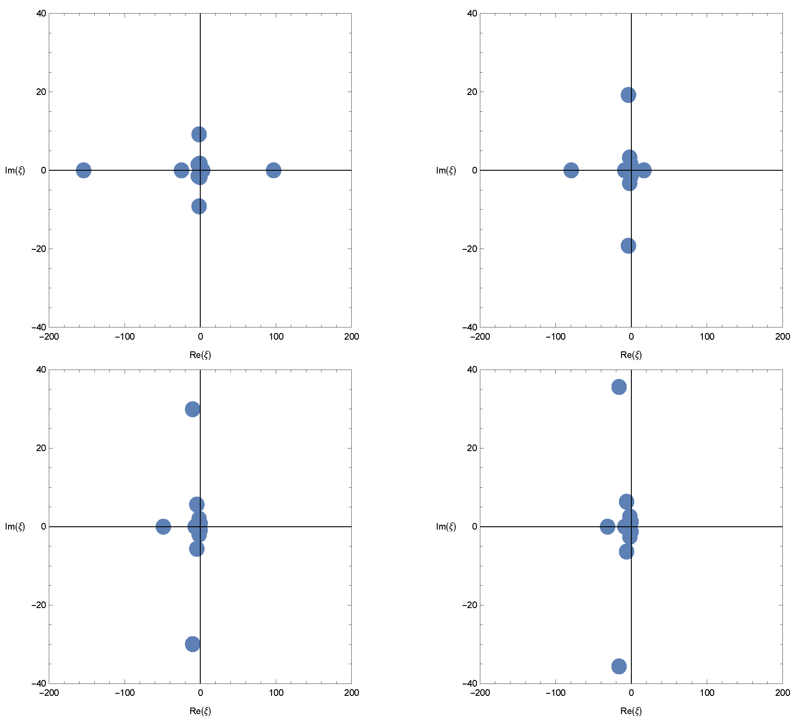
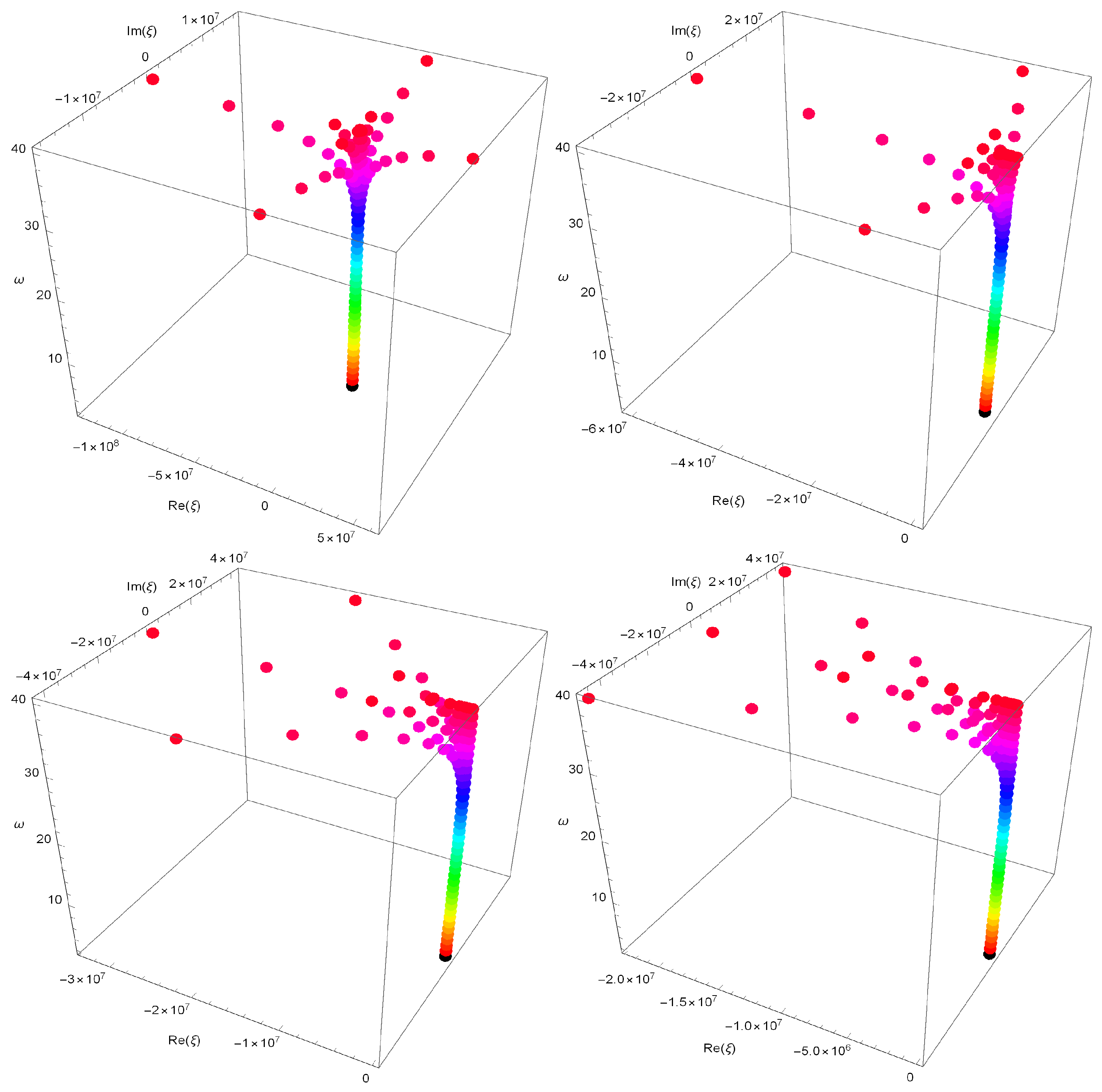
4. Approximate Roots for Cosine Apostol-Type Frobenius–Euler–Fibonacci Polynomials and Their Application

In this section, certain zeros of the two parametric kinds of cosine-Apostol-type Frobenius–Euler–Fibonacci polynomials ${\mathbb{H}}_{w,F}^{(\alpha ,c)}(\xi ,\nu ;u;\lambda )$ and beautifully graphical representations are shown.

A few of them are

$${\mathbb{H}}_{0,F}^{(\alpha ,c)}(\xi ,\nu ;u;\lambda )={\left(\frac{u-1}{u-\lambda }\right)}^{\alpha },$$

$${\mathbb{H}}_{1,F}^{(\alpha ,c)}(\xi ,\nu ;u;\lambda )=-\frac{u\xi {\left(\frac{-1+u}{u-\lambda }\right)}^{\alpha }}{-u+\lambda }+\frac{\xi {\left(\frac{-1+u}{u-\lambda }\right)}^{\alpha }\lambda }{-u+\lambda }-\frac{\alpha {\left(\frac{-1+u}{u-\lambda }\right)}^{\alpha }\lambda }{-u+\lambda },$$

$$\begin{array}{ccc}\hfill {\mathbb{H}}_{2,F}^{(\alpha ,c)}(\xi ,\nu ;u;\lambda )& =& {\xi }^2{\left(\frac{-1+u}{u-\lambda }\right)}^{\alpha }-{\nu }^2{\left(\frac{-1+u}{u-\lambda }\right)}^{\alpha }+\frac{u\alpha {\left(\frac{-1+u}{u-\lambda }\right)}^{\alpha }\lambda }{{(-u+\lambda )}^2}\hfill \\ & & -\frac{\alpha {\left(\frac{-1+u}{u-\lambda }\right)}^{\alpha }{\lambda }^2}{2{(-u+\lambda )}^2}+\frac{{\alpha }^2{\left(\frac{-1+u}{u-\lambda }\right)}^{\alpha }{\lambda }^2}{2{(-u+\lambda )}^2}-\frac{\xi \alpha {\left(\frac{-1+u}{u-\lambda }\right)}^{\alpha }\lambda }{-u+\lambda }\hfill \end{array}$$

and

$$\begin{array}{ccc}\hfill {\mathbb{H}}_{3,F}^{(\alpha ,c)}(\xi ,\nu ;u;\lambda )& =& {\xi }^3{\left(\frac{-1+u}{u-\lambda }\right)}^{\alpha }-2\xi {\nu }^2{\left(\frac{-1+u}{u-\lambda }\right)}^{\alpha }-\frac{u^2\alpha {\left(\frac{-1+u}{u-\lambda }\right)}^{\alpha }\lambda }{{(-u+\lambda )}^3}\hfill \\ & & -\frac{2u{\alpha }^2{\left(\frac{-1+u}{u-\lambda }\right)}^{\alpha }{\lambda }^2}{{(-u+\lambda )}^3}+\frac{\alpha {\left(\frac{-1+u}{u-\lambda }\right)}^{\alpha }{\lambda }^3}{3{(-u+\lambda )}^3}+\frac{{\alpha }^2{\left(\frac{-1+u}{u-\lambda }\right)}^{\alpha }{\lambda }^3}{{(-u+\lambda )}^3}\hfill \\ & & -\frac{{\alpha }^3{\left(\frac{-1+u}{u-\lambda }\right)}^{\alpha }{\lambda }^3}{3{(-u+\lambda )}^3}+\frac{2u\xi \alpha {\left(\frac{-1+u}{u-\lambda }\right)}^{\alpha }\lambda }{{(-u+\lambda )}^2}-\frac{\xi \alpha {\left(\frac{-1+u}{u-\lambda }\right)}^{\alpha }{\lambda }^2}{{(-u+\lambda )}^2}\hfill \\ & & +\frac{\xi {\alpha }^2{\left(\frac{-1+u}{u-\lambda }\right)}^{\alpha }{\lambda }^2}{{(-u+\lambda )}^2}-\frac{2{\xi }^2\alpha {\left(\frac{-1+u}{u-\lambda }\right)}^{\alpha }\lambda }{-u+\lambda }+\frac{2{\nu }^2\alpha {\left(\frac{-1+u}{u-\lambda }\right)}^{\alpha }\lambda }{-u+\lambda }.\hfill \end{array}$$

We investigate the beautiful zeros of the two parametric kinds of cosine-Apostol-type Frobenius–Euler–Fibonacci polynomials ${\mathbb{H}}_{w,F}^{(\alpha ,c)}(\xi ,\nu ;u;\lambda )=0$ using a computer. We plot the zeros of the two parametric kinds of cosine-Apostol-type Frobenius–Euler–Fibonacci polynomials ${\mathbb{H}}_{w,F}^{(\alpha ,c)}(\xi ,\nu ;u;\lambda )=0$ for $w=10$ (Figure 1).

In Figure 1 (top-left), we chose $\alpha =20,\lambda =3,u=40,$ and $\nu =\pi$. In Figure 1 (top-right), we chose $\alpha =20,\lambda =3,u=40,$ and $\nu =\frac{\pi }{2}$. In Figure 1 (bottom-left), we chose $\alpha =20,\lambda =3,u=40$, and $\nu =\frac{\pi }{3}$. In Figure 1 (bottom-right), we chose $\alpha =20,\lambda =3,u=40,$ and $\nu =\frac{\pi }{4}$.

Plots of real zeros of the two parametric kinds of cosine-Apostol-type Frobenius–Euler–Fibonacci polynomials ${\mathbb{H}}_{w,F}^{(\alpha ,c)}(\xi ,\nu ;u;\lambda )=0$ for $1\le w\le 40$ are presented (Figure 2).

In Figure 2 (top-left), we chose $\alpha =20,\lambda =3,u=40,$ and $\nu =\pi$. In Figure 2 (top-right), we chose $\alpha =20,\lambda =3,u=40,$ and $\nu =\frac{\pi }{2}$. In Figure 2 (bottom-left), we chose $\alpha =20,\lambda =3,u=40$, and $\nu =\frac{\pi }{3}$. In Figure 2 (bottom-right), we chose $\alpha =20,\lambda =3,u=40,$ and $\nu =\frac{\pi }{4}$.

Next, we calculated an approximate solution satisfying the two parametric kinds of cosine-Apostol-type Frobenius–Euler–Fibonacci polynomials ${\mathbb{H}}_{w,F}^{(\alpha ,c)}(\xi ,\nu ;u;\lambda )=0$ for $\alpha =20,\lambda =3,u=40,\nu =\frac{\pi }{3}$. The results are given in

Table 1. Approximate solutions of ${\mathbb{H}}_{w,F}^{(\alpha ,c)}(\xi ,\nu ;u;\lambda )=0$.

Degree w	$\mathit{\xi }$
1	−1.6216
2	−0.81081–1.11721i,   −0.81081 + 1.11721i
3	−2.5527,   −0.3453–1.3890i,   −0.3453 + 1.3890i
4	−2.1149 + 1.2065i,   −2.1149–1.2065i,
	−0.3176–1.6486i,   −0.3176 + 1.6486i
5	−4.9923,   −1.0243 + 2.8171i,   −1.0243–2.8171i,
	−0.53363–1.25377i,   −0.53363 + 1.25377i
6	−6.6054,   −2.8798,   −1.4002 + 4.3170i,
	−1.4002–4.3170i,   −0.34373 + 1.21593i,   −0.34373–1.21593i
7	−11.829,   −2.4479–7.1055i,   −2.4479 + 7.1055i,   −1.8300 + 1.8696i,
	−1.8300–1.8696i,   −0.34829 + 1.18791i,   −0.34829–1.18791i
8	−18.525,   −4.0494,   −3.8525–11.4136i,
	−3.8525 + 11.4136i,   −1.5458–2.4681i,   −1.5458 + 2.4681i,
	−0.34158 + 1.07275i,   −0.34158–1.07275i
9	−30.369,   −6.302 + 18.517i,   −6.302–18.517i,
	−3.8166 + 3.2636i,   −3.8166–3.2636i,   −1.9475–2.3368i,
	1.9475 + 2.3368i,   −0.31715 + 0.97703i,   −0.31715–0.97703i

.

5. Approximate Roots for Sine Apostol-Type Frobenius–Euler–Fibonacci Polynomials and Their Application

In this section, certain zeros of the two parametric kinds of sine-Apostol-type Frobenius–Euler–Fibonacci polynomials ${\mathbb{H}}_{w,F}^{(\alpha ,s)}(\xi ,\nu ;u;\lambda )=0$ and beautifully graphical representations are shown.

A few of them are

$${\mathbb{H}}_{0,F}^{(\alpha ,s)}(\xi ,\nu ;u;\lambda )=0,$$

$${\mathbb{H}}_{1,F}^{(\alpha ,s)}(\xi ,\nu ;u;\lambda )=\nu {\left(\frac{-1+u}{u-\lambda }\right)}^{\alpha },$$

$${\mathbb{H}}_{2,F}^{(\alpha ,s)}(\xi ,\nu ;u;\lambda )=-\frac{u\xi \nu {\left(\frac{-1+u}{u-\lambda }\right)}^{\alpha }}{-u+\lambda }+\frac{\xi \nu {\left(\frac{-1+u}{u-\lambda }\right)}^{\alpha }\lambda }{-u+\lambda }-\frac{\nu \alpha {\left(\frac{-1+u}{u-\lambda }\right)}^{\alpha }\lambda }{-u+\lambda },$$

$$\begin{array}{ccc}\hfill {\mathbb{H}}_{3,F}^{(\alpha ,s)}(\xi ,\nu ;u;\lambda )& =& 2{\xi }^2\nu {\left(\frac{-1+u}{u-\lambda }\right)}^{\alpha }-{\nu }^3{\left(\frac{-1+u}{u-\lambda }\right)}^{\alpha }+\frac{2u\nu \alpha {\left(\frac{-1+u}{u-\lambda }\right)}^{\alpha }\lambda }{{(-u+\lambda )}^2}\hfill \\ & & -\frac{\nu \alpha {\left(\frac{-1+u}{u-\lambda }\right)}^{\alpha }{\lambda }^2}{{(-u+\lambda )}^2}+\frac{\nu {\alpha }^2{\left(\frac{-1+u}{u-\lambda }\right)}^{\alpha }{\lambda }^2}{{(-u+\lambda )}^2}-\frac{2\xi \nu \alpha {\left(\frac{-1+u}{u-\lambda }\right)}^{\alpha }\lambda }{-u+\lambda }\hfill \end{array}$$

and

$$\begin{array}{ccc}\hfill {\mathbb{H}}_{4,F}^{(\alpha ,s)}(\xi ,\nu ;u;\lambda )& =& 3{\xi }^3\nu {\left(\frac{-1+u}{u-\lambda }\right)}^{\alpha }-3\xi {\nu }^3{\left(\frac{-1+u}{u-\lambda }\right)}^{\alpha }-\frac{3u^2\nu \alpha {\left(\frac{-1+u}{u-\lambda }\right)}^{\alpha }\lambda }{{(-u+\lambda )}^3}\hfill \\ & & -\frac{6u\nu {\alpha }^2{\left(\frac{-1+u}{u-\lambda }\right)}^{\alpha }{\lambda }^2}{{(-u+\lambda )}^3}+\frac{\nu \alpha {\left(\frac{-1+u}{u-\lambda }\right)}^{\alpha }{\lambda }^3}{{(-u+\lambda )}^3}+\frac{3\nu {\alpha }^2{\left(\frac{-1+u}{u-\lambda }\right)}^{\alpha }{\lambda }^3}{{(-u+\lambda )}^3}\hfill \\ & & -\frac{\nu {\alpha }^3{\left(\frac{-1+u}{u-\lambda }\right)}^{\alpha }{\lambda }^3}{{(-u+\lambda )}^3}+\frac{6u\xi \nu \alpha {\left(\frac{-1+u}{u-\lambda }\right)}^{\alpha }\lambda }{{(-u+\lambda )}^2}-\frac{3\xi \nu \alpha {\lambda }^2}{{(-u+\lambda )}^2}\hfill \\ & & +\frac{3\xi \nu {\alpha }^2{\left(\frac{-1+u}{u-\lambda }\right)}^{\alpha }{\lambda }^2}{{(-u+\lambda )}^2}-\frac{6{\xi }^2\nu \alpha {\left(\frac{-1+u}{u-\lambda }\right)}^{\alpha }\lambda }{-u+\lambda }+\frac{3{\nu }^3\alpha {\left(\frac{-1+u}{u-\lambda }\right)}^{\alpha }\lambda }{-u+\lambda }.\hfill \end{array}$$

We plot the zeros of the two parametric kinds of sine-Apostol-type Frobenius–Euler–Fibonacci polynomials ${\mathbb{H}}_{w,F}^{(\alpha ,s)}(\xi ,\nu ;u;\lambda )=0$ for $\omega =11$ (Figure 3).

In Figure 3 (top-left), we chose $\alpha =20,\lambda =3,u=40,$ and $\nu =\pi$. In Figure 3 (top-right), we chose $\alpha =20,\lambda =3,u=40,$ and $\nu =\frac{\pi }{2}$. In Figure 3 (bottom-left), we chose $\alpha =20,\lambda =3,u=40$, and $\nu =\frac{\pi }{3}$. In Figure 3 (bottom-right), we chose $\alpha =20,\lambda =3,u=40,$ and $\nu =\frac{\pi }{4}$.

Stacks of zeros of the two parametric kinds of sine-Apostol-type Frobenius–Euler–Fibonacci polynomials ${\mathbb{H}}_{w,F}^{(\alpha ,s)}(\xi ,\nu ;u;\lambda )=0$ for $3\le \omega \le 40$, forming a 3D structure, are presented (Figure 4).

In Figure 4 (top-left), we chose $\alpha =20,\lambda =3,u=40,$ and $\nu =\pi$. In Figure 4 (top-right), we chose $\alpha =20,\lambda =3,u=40,$ and $\nu =\frac{\pi }{2}$. In Figure 4 (bottom-left), we chose $\alpha =20,\lambda =3,u=40$, and $\nu =\frac{\pi }{3}$. In Figure 4 (bottom-right), we chose $\alpha =20,\lambda =3,u=40,$ and $\nu =\frac{\pi }{4}$.

Next, we calculated an approximate solution satisfying two parametric kinds of sine-Apostol-type Frobenius–Euler–Fibonacci polynomials ${\mathbb{H}}_{w,F}^{(\alpha ,s)}(\xi ,\nu ;u;\lambda )=0$ for $\alpha =20,\lambda =3,u=40,\nu =\frac{\pi }{4}$. The results are given in

Table 2. Approximate solutions of ${\mathbb{H}}_{w,F}^{(\alpha ,s)}(\xi ,\nu ;u;\lambda )=0$.

Degree w	$\mathit{\xi }$
2	−1.6216
3	−0.8108–1.4270i,   −0.8108 + 1.4270i
4	−2.3585,   −0.4424 + 1.7622i,   −0.4424–1.7622i
5	−1.8208–2.1580i,   −1.8208 + 2.1580i,
	−0.6117 + 1.8334i,   −0.6117–1.8334i
6	−3.7216,   −1.6884–3.8944i,   −1.6884 + 3.8944i,
	−0.5048–1.5492i,   −0.5048 + 1.5492i
7	−3.1006 + 2.3894i,   −3.1006–2.3894i,   −2.9654–5.8498i,
	−2.9654 + 5.8498i,   −0.4205–1.5019i,   −0.4205 + 1.5019i
8	−6.5500,   −4.6320–9.7962i,   −4.6320 + 9.7962i,   −2.2337 + 2.8199i,
	−2.2337–2.8199i,   −0.3998–1.4437i,   −0.3998 + 1.4437i
9	−7.590–15.664i,   −7.590 + 15.664i,   −6.9050–3.0783i,
	−6.9050 + 3.0783i,   −2.1598–2.9826i,   −2.1598 + 2.9826i,
	−0.3719–1.3842i,   −0.3719 + 1.3842i
10	−13.328,   −12.221–25.464i,   −12.221 + 25.464i,
	−6.2140 + 5.1861i,   −6.2140–5.1861i,   −2.1195–2.7752i,
	−2.1195 + 2.7752i,   −0.34922 + 1.33983i,   −0.34922–1.33983i

.

6. Conclusions

The employment of special polynomials in scientific fields is extensive and diverse, encompassing areas such as signal processing, geoscience, engineering, and quantum mechanics. These polynomials play a crucial role in numerical analysis and computational techniques, facilitating the resolution of intricate issues spanning various scientific domains. In numerous studies, researchers in the field of applied mathematics have utilized generating functions and function equations of special polynomials to investigate various topics. The results of these investigations have been documented in numerous research papers. In this article, we aim to introduce the F-analogues of the Apostol-type Frobenius–Euler polynomials defined by Kılar and Simsek [22], using Golden calculus. We have obtained several fundamental properties of these newly established polynomials. Some of the main results in the paper generalize the recently published paper [23]. Furthermore, we have provided zeroes and graphical illustrations for the parametric kinds of Apostol-type Frobenius–Euler–Fibonacci polynomials. The results of this article have the potential to motivate researchers and readers to conduct further research on these special numbers and polynomials.

References

1. Alam, N.; Khan, W.A.; Ryoo, C.S. A note on Bell-based Apostol-type Frobenius-Euler polynomials of complex variable with its certain applications. Mathematics 2022, 10, 2109. [Google Scholar] [CrossRef]
2. Lyapin, A.P.; Akhtamova, S.S. Recurrence relations for the sections of the generating series of the solution to the multidimensional difference equation. Vestn. Udmurtsk. Univ. Mat. Mekh. 2021, 31, 414–423. [Google Scholar] [CrossRef]
3. Carlitz, L. Eulerian numbers and polynomials. Mat. Mag. 1959, 32, 164–171. [Google Scholar] [CrossRef]
4. Cakić, N.P.; Milovanović, G.V. On generalized Stirling number and polynomials. Math. Balk. N. Ser. 2004, 18, 241–248. [Google Scholar]
5. Luo, Q.M.; Srivastava, H.M. Some generalization of the Apostol-Genocchi polynomials and Stirling numbers of the second kind. Appl. Math. Comput. 2011, 217, 5702–5728. [Google Scholar] [CrossRef]
6. Kurt, B.; Simsek, Y. On the generalized Apostol-type Frobenius-Euler polynomials. Adv. Differ. Equ. 2013, 2013, 1. [Google Scholar] [CrossRef]
7. Kim, D.S.; Kim, T. Some new identities of Frobenius-Euler numbers and polynomials. J. Inequal. Appl. 2012, 2012, 307. [Google Scholar] [CrossRef]
8. Ryoo, C.S. A note on the Frobenius Euler polynomials. Proc. Jangjeon Math. Soc. 2011, 14, 495–501. [Google Scholar]
9. Luo, Q.M.; Srivastava, H.M. Some generalizations of the Apostol-Bernoulli and Apostol-Euler polynomials. J. Math. Anal. Appl. 2005, 308, 290–302. [Google Scholar] [CrossRef]
10. Jamei, M.J.; Milovanović, G.; Dagli, M.C. A generalization of the array type polynomials. Math. Morav. 2022, 26, 37–46. [Google Scholar] [CrossRef]
11. Simsek, Y. Generating functions for generalized Stirling type numbers, Array type polynomials, Eulerian type polynomials and their applications. J. Fixed Point Theory Appl. 2013, 2013, 87. [Google Scholar] [CrossRef]
12. Kus, S.; Tuglu, N.; Kim, T. Bernoulli F-polynomials and Fibo-Bernoulli matrices. Adv. Differ. Equ. 2019, 2019, 145. [Google Scholar] [CrossRef]
13. Özvatan, M. Generalized Golden-Fibonacci Calculus and Applications. Ph.D. Thesis, Izmir Institute of Technology, Urla/Izmir, Turkey, 2018. [Google Scholar]
14. Pashaev, O.K.; Nalci, S. Golden quantum oscillator and Binet–Fibonacci calculus. J. Phys. A Math. Theor. 2012, 45, 23. [Google Scholar] [CrossRef]
15. Pashaev, O.K. Quantum calculus of Fibonacci divisors and infinite hierarchy of bosonic-fermionic golden quantum oscillators. Internat. J. Geom. Methods Modern Phys. 2021, 18, 32. [Google Scholar] [CrossRef]
16. Krot, E. An introduction to finite fibonomial calculus. Centr. Eur. J. Math. 2004, 2, 754–766. [Google Scholar] [CrossRef]
17. Pashaev, O.K.; Ozvatan, M. Bernoulli-Fibonacci Polynomials. arXiv 2020, arXiv:2010.15080. [Google Scholar]
18. Gulal, E.; Tuglu, N. Apostol-Bernoulli-Fibonacci polynomials, Apostol-Euler-Fibonacci polynomials and their generating functions. Turk. J. Math. Comput. Sci. 2023, 15, 202–210. [Google Scholar] [CrossRef]
19. Kızılateş, C.; Öztürk, H. On parametric types of Apostol Bernoulli-Fibonacci Apostol Euler-Fibonacci and Apostol Genocchi-Fibonacci polynomials via Golden calculus. AIMS Math. 2023, 8, 8386–8402. [Google Scholar] [CrossRef]
20. Tuğlu, N.; Ercan, E. Some properties of Apostol Bernoulli Fibonacci and Apostol Euler Fibonacci Polynomials. In Proceedings of the ICMEE-2021, Ankara, Turkey, 16–18 September 2021; pp. 32–34. [Google Scholar]
21. Alatawi, M.A.; Khan, W.A.; Kızılateş, C.; Ryoo, C.S. Some Properties of Generalized Apostol-type Frobenius-Euler-Fibonacci polynomials. Mathematics 2024, 12, 800. [Google Scholar] [CrossRef]
22. Kılar, N.; Simsek, Y. Two Parametric Kinds of Eulerian-Type Polynomials Associated with Euler’s Formula. Symmetry 2019, 11, 1097. [Google Scholar] [CrossRef]
23. Urieles, A.; Ramirez, W.; Ha, L.C.P.; Ortegac, M.J.; Arenas-Penaloza, J. On F-Frobenius-Euler polynomials and their matrix approach. J. Math. Comput. Sci. 2024, 32, 377–386. [Google Scholar] [CrossRef]
Figure 1. Zeros of H w , F ( α , c ) ( ξ , ν ; u ; λ ) = 0 .
Axioms 13 00348 g001
Figure 2. Real zeros of H w , F ( α , c ) ( ξ , ν ; u ; λ ) = 0 .
Axioms 13 00348 g002
Figure 3. Zeros of H w , F ( α , s ) ( ξ , ν ; u ; λ ) = 0 .
Axioms 13 00348 g003
Figure 4. Zeros of H w , F ( α , s ) ( ξ , ν ; u ; λ ) = 0 .
Axioms 13 00348 g004